Multisymplectic Geometry, Variational Integrators, and Nonlinear PDEs

Abstract

This paper presents a geometric-variational approach to continuous and discrete mechanics and field theories. Using multisymplectic geometry, we show that the existence of the fundamental geometric structures as well as their preservation along solutions can be obtained directly from the variational principle. In particular, we prove that a unique multisymplectic structure is obtained by taking the derivative of an action function, and use this structure to prove covariant generalizations of conservation of symplecticity and Noether’s theorem. Natural discretization schemes for PDEs, which have these important preservation properties, then follow by choosing a discrete action functional. In the case of mechanics, we recover the variational symplectic integrators of Veselov type, while for PDEs we obtain covariant spacetime integrators which conserve the corresponding discrete multisymplectic form as well as the discrete momentum mappings corresponding to symmetries. We show that the usual notion of symplecticity along an infinite-dimensional space of fields can be naturally obtained by making a spacetime split. All of the aspects of our method are demonstrated with a nonlinear sine-Gordon equation, including computational results and a comparison with other discretization schemes.

1 Introduction

The purpose of this paper is to develop the geometric foundations for multisymplectic-momentum integrators for variational partial differential equations (PDEs). These integrators are the PDE generalizations of symplectic integrators that are popular for Hamiltonian ODEs (see, for example, the articles in Marsden, Patrick and Shadwick [1996], and especially the review article of McLachlan and Scovel [1996]) in that they are covariant spacetime integrators which preserve the geometric structures of the system.

Because of the covariance of our method which we shall describe below, the resulting integrators are spacetime localizable in the context of hyperbolic PDEs, and generalize the notion of symplecticity and symmetry preservation in the context of elliptic problems. Herein, we shall primarily focus on spacetime integrators; however, we shall remark on the connection of our method with the finite element method for elliptic problems, as well as the Gregory and Lin [1991] method in optimal control.

Historically, in the setting of ODEs, there have been many approaches devised for constructing symplectic integrators, beginning with the original derivations based on generating functions (see de Vogelaere [1956]) and proceeding to symplectic Runge-Kutta algorithms, the shake algorithm, and many others. In fact, in many areas of molecular dynamics, symplectic integrators such as the Verlet algorithm and variants thereof are quite popular, as are symplectic integrators for the integration of the solar system. In these domains, integrators that are either symplectic or which are adaptations of symplectic integrators, are amongst the most widely used.

A fundamentally new approach to symplectic integration is that of Veselov [1988], [1991] who developed a discrete mechanics based on a discretization of Hamilton’s principle. Their method leads in a natural way to symplectic-momentum integrators which include the shake and Verlet integrators as special cases (see Wendlandt and Marsden [1997]). In addition, Veselov integrators often have amazing properties with regard to preservation of integrable structures, as has been shown by Moser and Veselov [1991]. This aspect has yet to be exploited numerically, but it seems to be quite important.

The approach we take in this paper is to develop a Veselov-type discretization for PDE’s in variational form. The relevant geometry for this situation is multisymplectic geometry (see Gotay, Isenberg, and Marsden [1997] and Marsden and Shkoller [1997]) and we develop it in a variational framework. As we have mentioned, this naturally leads to multisymplectic-momentum integrators. It is well-known that such integrators cannot in general preserve the Hamiltonian exactly (Ge and Marsden [1988]). However, these integrators have, under appropriate circumstances, very good energy performance in the sense of the conservation of a nearby Hamiltonian up to exponentially small errors, assuming small time steps, due to a result of Neishtadt [1984]. See also Dragt and Finn [1979], and Simo and Gonzales [1993]. This is related to backward error analysis; see Sanz-Serna and Calvo [1994], Calvo and Hairer [1995], and the recent work of Hyman, Newman and coworkers and references therein. It would be quite interesting to develop the links with Neishtadt’s analysis more thoroughly.

An important part of our approach is to understand how the symplectic nature of the integrators is implied by the variational structure. In this way we are able to identify the symplectic and momentum conserving properties after discretizing the variational principle itself. Inspired by a paper of Wald [1993], we obtain a formal method for locating the symplectic or multisymplectic structures directly from the action function and its derivatives. We present the method in the context of ordinary Lagrangian mechanics, and apply it to discrete Lagrangian mechanics, and both continuous and discrete multisymplectic field theory. While in these contexts our variational method merely uncovers the well-known differential-geometric structures, our method forms an excellent pedagogical approach to those theories.

Outline of paper.

• In this section we sketch the three main aspects of our variational approach in the familiar context of particle mechanics. We show that the usual symplectic $2$-form on the tangent bundle of the configuration manifold arises naturally as the boundary term in the first variational principle. We then show that application of $d^{2}=0$ to the variational principle restricted to the space of solutions of the Euler-Lagrange equations produces the familiar concept of conservation of the symplectic form; this statement is obtained variationally in a non-dynamic context; that is, we do not require an evolutionary flow. We then show that if the action function is left invariant by a symmetry group, then Noether’s theorem follows directly and simply from the variational principle as well.

• Here we use our variational approach to construct discretization schemes for mechanics which preserve the discrete symplectic form and the associated discrete momentum mappings.

• This section defines the three aspects of our variational approach in the multisymplectic field-theoretic setting. Unlike the traditional approach of defining the canonical multisymplectic form on the dual of the first jet bundle and then pulling back to the Lagrangian side using the covariant Legendre transform, we obtain the geometric structure by staying entirely on the Lagrangian side. We prove the covariant analogue of the fact that the flow of conservative systems consists of symplectic maps; we call this result the multisymplectic form formula. After variationally proving a covariant version of Noether’s theorem, we show that one can use the multisymplectic form formula to recover the usual notion of symplecticity of the flow in an infinite-dimensional space of fields by making a spacetime split. We demonstrate this machinery using a nonlinear wave equation as an example.

• In this section we develop discrete field theories from which the covariant integrators follow. We define discrete analogues of the first jet bundle of the configuration bundle whose sections are the fields of interest, and proceed to define the discrete action sum. We then apply our variational algorithm to this discrete action function to produce the discrete Euler-Lagrange equations and the discrete multisymplectic forms. As a consequence of our methodology, we show that the solutions of the discrete Euler-Lagrange equations satisfy the discrete version of the multisymplectic form formula as well as the discrete version of our generalized Noether’s theorem. Using our nonlinear wave equation example, we develop various multisymplectic-momentum integrators for the sine-Gordon equations, and compare our resulting numerical scheme with the energy-conserving methods of Li and Vu-Quoc [1995] and Guo, Pascual, Rodriguez, and Vazquez [1986]. Results are presented for long-time simulations of kink-antikink solutions for over 5000 soliton collisions.

• This section contains some important remarks concerning the variational integrator methodology. For example, we discuss integrators for reduced systems, the role of grid uniformity, and the interesting connections with the finite-element methods for elliptic problems. We also make some comments on future work.

2 Lagrangian Mechanics

Hamilton’s Principle.

We begin by recalling a problem going back to Euler, Lagrange and Hamilton in the period 1740–1830. Consider an $n$-dimensional configuration manifold $Q$ with its tangent bundle $TQ$. We denote coordinates on $Q$ by $q^{i}$ and those on $TQ$ by $(q^{i},\dot{q}^{i})$. Consider a Lagrangian $L:TQ\rightarrow\mathbb{R}$. Construct the corresponding action functional $S$ on $C^{2}$ curves $q(t)$ in $Q$ by integration of $L$ along the tangent to the curve. In coordinate notation, this reads

$$S\bigl{(}q(t)\bigr{)}\equiv\int_{a}^{b}L\left(q^{i}(t),\frac{dq^{i}}{dt}(t)\right)\,dt.$$ (2.1)

The action functional depends on $a$ and $b$, but this is not explicit in the notation. Hamilton’s principle seeks the curves $q(t)$ for which the functional $S$ is stationary under variations of $q(t)$ with fixed endpoints; namely, we seek curves $q(t)$ which satisfy

$$dS\bigl{(}q(t)\bigr{)}\cdot\delta q(t)\equiv{\displaystyle\left.\frac{d}{d\epsilon}\right|_{\epsilon=0}}S\bigl{(}q_{\epsilon}(t)\bigr{)}=0$$ (2.2)

for all $\delta q(t)\text{ with }\delta q(a)=\delta q(b)=0$, where $q_{\epsilon}$ is a smooth family of curves with $q_{0}=q$ and $(d/d\epsilon)|_{\epsilon=0}q_{\epsilon}=\delta q$. Using integration by parts, the calculation for this is simply

$$dS\bigl{(}q(t)\bigr{)}\cdot\delta q(t) = {\displaystyle\left.\frac{d}{d\epsilon}\right|_{\epsilon=0}}\int_{a}^{b}L\left(q_{\epsilon}^{i}(t),\frac{dq_{\epsilon}^{i}}{dt}(t)\right)\,dt$$ (2.3)

$$= \int_{a}^{b}\delta q^{i}\left(\frac{\partial L}{\partial q^{i}}-\frac{d}{dt}\frac{\partial L}{\partial\dot{q}^{i}}\right)dt+\left.\frac{\partial L}{\partial\dot{q}^{i}}\delta q^{i}\right|_{a}^{b}.$$

The last term in (2.3) vanishes since $\delta q(a)=\delta q(b)=0$, so that the requirement (2.2) for $S$ to be stationary yields the Euler-Lagrange equations

$$\frac{\partial L}{\partial q^{i}}-\frac{d}{dt}\frac{\partial L}{\partial\dot{q}^{i}}=0.$$ (2.4)

Recall that $L$ is called regular when the symmetric matrix $[\partial^{2}L/\partial\dot{q}^{i}\partial\dot{q}^{j}]$ is everywhere nonsingular. If $L$ is regular, the Euler-Lagrange equations are second order ordinary differential equations for the required curves.

The standard geometric setting.

The action (2.1) is independent of the choice of coordinates, and thus the Euler-Lagrange equations are coordinate independent as well. Consequently, it is natural that the Euler-Lagrange equations may be intrinsically expressed using the language of differential geometry. This intrinsic development of mechanics is now standard, and can be seen, for example, in Arnold [1978], Abraham and Marsden [1978], and Marsden and Ratiu [1994].

The canonical $1$-form $\theta_{0}$ on the $2n$-dimensional cotangent bundle of $Q$, $T^{*}Q$ is defined by

$$\theta_{0}(\alpha_{q})w_{\alpha_{q}}\equiv\alpha_{q}\cdot T\pi_{Q}w_{\alpha_{q}},\qquad\mbox{$\alpha_{q}\in T^{*}_{q}Q$, $w_{\alpha_{q}}\in T_{\alpha_{q}}T^{*}Q$},$$

where $\pi_{Q}:T^{*}Q\rightarrow Q$ is the canonical projection. The Lagrangian $L$ intrinsically defines a fiber preserving bundle map $\mathbb{F}L:TQ\rightarrow T^{*}Q$, the Legendre transformation, by vertical differentiation:

$$\mathbb{F}L(v_{q})w_{q}\equiv{\displaystyle\left.\frac{d}{d\epsilon}\right|_{\epsilon=0}}L(v_{q}+\epsilon w_{q}).$$

We define the Lagrange $1$-form on $TQ$, the Lagrangian side, by pull-back $\theta_{L}\equiv\mathbb{F}L^{*}\theta_{0}$, and the Lagrange $2$-form by $\omega_{L}=-d\theta_{L}$. We then seek a vector field $X_{E}$ (called the Lagrange vector field) on $TQ$ such that $X_{E}\mathbin{\hbox to6.0pt{\vrule height=0.4pt,width=5.0pt,depth=0.0pt\kern-0.4pt\vrule height=6.0pt,width=0.4pt,depth=0.0pt\hss}}\omega_{L}=dE$, where the energy $E$ is defined by $E(v_{q})\equiv\mathbb{F}L(v_{q})v_{q}-L(v_{q})$.

If $\mathbb{F}L$ is a local diffeomorphism then $X_{E}$ exists and is unique, and its integral curves solve the Euler-Lagrange equations (2.4). In addition, the flow $F_{t}$ of $X_{E}$ preserves $\omega_{L}$; that is, $F_{t}^{*}\omega_{L}=\omega_{L}$. Such maps are symplectic, and the form $\omega_{L}$ is called a symplectic $2$-form. This is an example of a symplectic manifold: a pair $(M,\omega)$ where $M$ is a manifold and $\omega$ is closed nondegenerate $2$-form.

Despite the compactness and precision of this differential-geometric approach, it is difficult to motivate and, furthermore, is not entirely contained on the Lagrangian side. The canonical $1$-form $\theta_{0}$ seems to appear from nowhere, as does the Legendre transform $\mathbb{F}L$. Historically, after the Lagrangian picture on $TQ$ was constructed, the canonical picture on $T^{*}Q$ emerged through the work of Hamilton, but the modern approach described above treats the relation between the Hamiltonian and Lagrangian pictures of mechanics as a mathematical tautology, rather than what it is—a discovery of the highest order.

The variational approach.

More and more, one is finding that there are advantages to staying on the “Lagrangian side”. Many examples can be given, but the theory of Lagrangian reduction (the Euler-Poincaré equations being an instance) is one example (see, for example, Marsden and Ratiu [1994] and Holm, Marsden and Ratiu [1998a,b]); another, of many, is the direct variational approach to questions in black hole dynamics given by Wald [1993]. In such studies, it is the variational principle that is the center of attention.

We next show that one can derive in a natural way the fundamental differential geometric structures, including momentum mappings, directly from the variational approach. This development begins by removing the boundary condition $\delta q(a)=\delta q(b)=0$ from (2.3). Equation (2.3) becomes

$$dS\bigl{(}q(t)\bigr{)}\cdot\delta q(t)=\int_{a}^{b}\delta q^{i}\left(\frac{\partial L}{\partial q^{i}}-\frac{d}{dt}\frac{\partial L}{\partial\dot{q}^{i}}\right)dt+\left.\frac{\partial L}{\partial\dot{q}^{i}}\delta q^{i}\right|_{a}^{b},$$ (2.5)

where the left side now operates on more general $\delta q$ (this generalization will be described in detail in Section (4)), while the last term on the right side does not vanish. That last term of (2.5) is a linear pairing of the function $\partial L/\partial\dot{q}^{i}$, a function of $q^{i}$ and $\dot{q}^{i}$, with the tangent vector $\delta q^{i}$. Thus, one may consider it to be a $1$-form on $TQ$; namely the $1$-form $(\partial L/\partial\dot{q}^{i})dq^{i}$. This is exactly the Lagrange $1$-form, and we can turn this into a formal theorem/definition:

Theorem 2.1

Given a $C^{k}$ Lagrangian $L$, $k\geq 2$, there exists a unique $C^{k-2}$ mapping $D_{\mbox{\scriptsize EL}}L:\ddot{Q}\rightarrow T^{*}Q$, defined on the second order submanifold

$$\ddot{Q}\equiv\left\{\left.\frac{d^{2}q}{dt^{2}}(0)\;\right|\;\mbox{$q$ a $C^{2}$ curve in $Q$}\right\}$$

of $TTQ$, and a unique $C^{k-1}$ $1$-form $\theta_{L}$ on $TQ$, such that, for all $C^{2}$ variations $q_{\epsilon}(t)$,

$$dS\bigl{(}q(t)\bigr{)}\cdot\delta q(t)=\int_{a}^{b}D_{\mbox{\scriptsize EL}}L\left(\frac{d^{2}q}{dt^{2}}\right)\cdot\delta q\,dt+\left.\theta_{L}\left(\frac{dq}{dt}\right)\cdot\hat{\delta q}\right|_{a}^{b},$$ (2.6)

where

$$\delta q(t)\equiv{\displaystyle\left.\frac{d}{d\epsilon}\right|_{\epsilon=0}}q_{\epsilon}(t),\qquad\hat{\delta q}(t)\equiv{\displaystyle\left.\frac{d}{d\epsilon}\right|_{\epsilon=0}}{\displaystyle\left.\frac{d}{dt}\right|_{t=0}}q_{\epsilon}(t).$$

The $1$-form so defined is called the Lagrange $1$-form.

Indeed, uniqueness and local existence follow from the calculation (2.3), and the coordinate independence of the action, and then global existence is immediate. Here then, is the first aspect of our method:

Using the variational principle, the Lagrange $1$-form $\theta_{L}$ is the “boundary part” of the the functional derivative of the action when the boundary is varied. The analogue of the symplectic form is the (negative of) the exterior derivative of $\theta_{L}$.

For the mechanics example being discussed, we imagine a development wherein $\theta_{L}$ is so defined and we define $\omega_{L}\equiv-d\theta_{L}$.

Lagrangian flows are symplectic.

One of Lagrange’s basic discoveries was that the solutions of the Euler-Lagrange equations give rise to a symplectic map. It is a curious twist of history that he did this without the machinery of either differential forms, of the Hamiltonian formalism or of Hamilton’s principle itself. (See Marsden and Ratiu [1994] for an account of some of this history.)

Assuming that $L$ is regular, the variational principle then gives coordinate independent second order ordinary differential equations, as we have noted. We temporarily denote the vector field on $TQ$ so obtained by $X$, and its flow by $F_{t}$. Our further development relies on a change of viewpoint: we focus on the restriction of $S$ to the subspace $\mathcal{C}_{L}$ of solutions of the variational principle. The space $\mathcal{C}_{L}$ may be identified with the initial conditions, elements of $TQ$, for the flow: to $v_{q}\in TQ$, we associate the integral curve $s\mapsto F_{s}(v_{q})$, $s\in[0,t]$. The value of $S$ on that curve is denoted by $S_{t}$, and again called the action. Thus, we define the map $S_{t}:TQ\rightarrow\mathbb{R}$ by

$$S_{t}(v_{q})=\int_{0}^{t}L(q(s),\dot{q}(s))\,ds,$$ (2.7)

where $(q(s),\dot{q}(s))=F_{s}(v_{q})$. The fundamental equation (2.6) becomes

$$dS_{t}(v_{q})w_{v_{q}}=\theta_{L}\bigl{(}F_{t}(v_{q})\bigr{)}\cdot{\displaystyle\left.\frac{d}{d\epsilon}\right|_{\epsilon=0}}F_{t}(v_{q}^{\epsilon})-\theta_{L}(v_{q})\cdot w_{v_{q}},$$

where $\epsilon\mapsto v_{q}^{\epsilon}$ is an arbitrary curve in $TQ$ such that $v_{q}^{0}=v_{q}$ and $(d/d\epsilon)|_{0}v^{\epsilon}_{q}=w_{v_{q}}$. We have thus derived the equation

$$dS_{t}=F_{t}^{*}\theta_{L}-\theta_{L}.$$ (2.8)

Taking the exterior derivative of (2.8) yields the fundamental fact that the flow of $X$ is symplectic:

$$0=ddS_{t}=d(F_{t}^{*}\theta_{L}-\theta_{L})=-F_{t}^{*}\omega_{L}+\omega_{L}$$

which is equivalent to

$$F_{t}^{*}\omega_{L}=\omega_{L}.$$

This leads to the following:

Using the variational principle, the fact that the evolution is symplectic is a consequence of the equation $d^{2}=0$, applied to the action restricted to the space of solutions of the variational principle.

In passing, we note that (2.8) also provides the differential-geometric equations for $X$. Indeed, one time derivative of (2.8) and using (2.7) gives $dL={\mathfrak{L}}_{X}\theta_{\mathcal{L}}$, so that

$$X\mathbin{\hbox to6.0pt{\vrule height=0.4pt,width=5.0pt,depth=0.0pt\kern-0.4pt\vrule height=6.0pt,width=0.4pt,depth=0.0pt\hss}}\omega_{L}=-X\mathbin{\hbox to6.0pt{\vrule height=0.4pt,width=5.0pt,depth=0.0pt\kern-0.4pt\vrule height=6.0pt,width=0.4pt,depth=0.0pt\hss}}d\theta_{L}=-{\mathfrak{L}}_{X}\theta_{L}+d(X\mathbin{\hbox to6.0pt{\vrule height=0.4pt,width=5.0pt,depth=0.0pt\kern-0.4pt\vrule height=6.0pt,width=0.4pt,depth=0.0pt\hss}}\theta_{L})=d(X\mathbin{\hbox to6.0pt{\vrule height=0.4pt,width=5.0pt,depth=0.0pt\kern-0.4pt\vrule height=6.0pt,width=0.4pt,depth=0.0pt\hss}}\theta_{L}-L)=dE,$$

if we define $E\equiv X\mathbin{\hbox to6.0pt{\vrule height=0.4pt,width=5.0pt,depth=0.0pt\kern-0.4pt\vrule height=6.0pt,width=0.4pt,depth=0.0pt\hss}}\theta_{L}-L$. Thus, we quite naturally find that $X=X_{E}$.

Of course, this set up also leads directly to Hamilton-Jacobi theory, which was one of the ways in which symplectic integrators were developed (see McLachlan and Scovel [1996] and references therein.) However, we shall not pursue the Hamilton-Jacobi aspect of the theory here.

Momentum maps.

Suppose that a Lie group $G$, with Lie algebra $\mathfrak{g}$, acts on $Q$, and hence on curves in $Q$, in such a way that the action $S$ is invariant. Clearly, $G$ leaves the set of solutions of the variational principle invariant, so the action of $G$ restricts to $\mathcal{C}_{L}$, and the group action commutes with $F_{t}$. Denoting the infinitesimal generator of $\xi\in\mathfrak{g}$ on $TQ$ by $\xi_{TQ}$, we have by (2.8),

$$0=\xi_{TQ}\mathbin{\hbox to6.0pt{\vrule height=0.4pt,width=5.0pt,depth=0.0pt\kern-0.4pt\vrule height=6.0pt,width=0.4pt,depth=0.0pt\hss}}dS_{t}=\xi_{TQ}\mathbin{\hbox to6.0pt{\vrule height=0.4pt,width=5.0pt,depth=0.0pt\kern-0.4pt\vrule height=6.0pt,width=0.4pt,depth=0.0pt\hss}}(F_{t}^{*}\theta_{L}-\theta_{L})=F_{t}^{*}(\xi_{TQ}\mathbin{\hbox to6.0pt{\vrule height=0.4pt,width=5.0pt,depth=0.0pt\kern-0.4pt\vrule height=6.0pt,width=0.4pt,depth=0.0pt\hss}}\theta_{L})-\xi_{TQ}\mathbin{\hbox to6.0pt{\vrule height=0.4pt,width=5.0pt,depth=0.0pt\kern-0.4pt\vrule height=6.0pt,width=0.4pt,depth=0.0pt\hss}}\theta_{L}.$$ (2.9)

For $\xi\in\mathfrak{g}$, define $J_{\xi}:TQ\rightarrow\mathbb{R}$ by $J_{\xi}\equiv\xi_{TQ}\mathbin{\hbox to6.0pt{\vrule height=0.4pt,width=5.0pt,depth=0.0pt\kern-0.4pt\vrule height=6.0pt,width=0.4pt,depth=0.0pt\hss}}\theta_{L}$. Then (2.9) says that $J_{\xi}$ is an integral of the flow of $X_{E}$. We have arrived at a version of Noether’s theorem (rather close to the original derivation of Noether):

Using the variational principle, Noether’s theorem results from the infinitesimal invariance of the action restricted to space of solutions of the variational principle. The conserved momentum associated to a Lie algebra element $\xi$ is $J_{\xi}=\xi_{TQ}\mathbin{\hbox to6.0pt{\vrule height=0.4pt,width=5.0pt,depth=0.0pt\kern-0.4pt\vrule height=6.0pt,width=0.4pt,depth=0.0pt\hss}}\theta_{L}$, where $\theta_{L}$ is the Lagrange one-form.

Reformulation in terms of first variations.

We have just seen that symplecticity of the flow and Noether’s theorem result from restricting the action to the space of solutions. One tacit assumption is that the space of solutions is a manifold in some appropriate sense. This is a potential problem, since solution spaces for field theories are known to have singularities (see, e.g., Arms, Marsden and Moncrief [1982]). More seriously there is the problem of finding a multisymplectic analogue of the statement that the Lagrangian flow map is symplectic, since for multisymplectic field theory one obtains an evolution picture only after splitting spacetime into space and time and adopting the “function space” point of view. Having the general formalism depend either on a spacetime split or an analysis of the associated Cauchy problem would be contrary to the general thrust of this article. We now give a formal argument, in the context of Lagrangian mechanics, which shows how both these problems can be simultaneously avoided.

Given a solution $q(t)\in\mathcal{C}_{L}$, a first variation at $q(t)$ is a vector field $V$ on $Q$ such that $t\mapsto F^{V}_{\epsilon}\circ q(t)$ is also a solution curve (i.e. a curve in $\mathcal{C}_{L}$). We think of the solution space $\mathcal{C}_{L}$ as being a (possibly) singular subset of the smooth space of all putative curves $\mathcal{C}$ in $TQ$, and the restriction of $V$ to $q(t)$ as being the derivative of some curve in $\mathcal{C}_{L}$ at $q(t)$. When $\mathcal{C}_{L}$ is a manifold, a first variation is a vector at $q(t)$ tangent to $\mathcal{C}_{L}$. Temporarily define $\alpha\equiv dS-\theta_{L}$ where by abuse of notation $\theta_{L}$ is the one form on $\mathcal{C}$ defined by

$$\theta_{L}\bigl{(}q(t)\bigr{)}\delta q(t)\equiv\theta_{L}(b)\delta q(b)-\theta_{L}(a)\delta q(a).$$

Then $\mathcal{C}_{L}$ is defined by $\alpha=0$ and we have the equation

$$dS=\alpha+\theta_{L},$$

so if $V$ and $W$ are first variations at $q(t)$, we obtain

$$0=V\mathbin{\hbox to6.0pt{\vrule height=0.4pt,width=5.0pt,depth=0.0pt\kern-0.4pt\vrule height=6.0pt,width=0.4pt,depth=0.0pt\hss}}W\mathbin{\hbox to6.0pt{\vrule height=0.4pt,width=5.0pt,depth=0.0pt\kern-0.4pt\vrule height=6.0pt,width=0.4pt,depth=0.0pt\hss}}d^{2}S=V\mathbin{\hbox to6.0pt{\vrule height=0.4pt,width=5.0pt,depth=0.0pt\kern-0.4pt\vrule height=6.0pt,width=0.4pt,depth=0.0pt\hss}}W\mathbin{\hbox to6.0pt{\vrule height=0.4pt,width=5.0pt,depth=0.0pt\kern-0.4pt\vrule height=6.0pt,width=0.4pt,depth=0.0pt\hss}}d\alpha+V\mathbin{\hbox to6.0pt{\vrule height=0.4pt,width=5.0pt,depth=0.0pt\kern-0.4pt\vrule height=6.0pt,width=0.4pt,depth=0.0pt\hss}}W\mathbin{\hbox to6.0pt{\vrule height=0.4pt,width=5.0pt,depth=0.0pt\kern-0.4pt\vrule height=6.0pt,width=0.4pt,depth=0.0pt\hss}}d\theta_{L}.$$ (2.10)

We have the identity

$$d\alpha(V,W)\bigl{(}q(t)\bigr{)}=V\bigl{(}\alpha(W)\bigr{)}-W\bigl{(}\alpha(V)\bigr{)}-\alpha([V,W]),$$ (2.11)

which we will use to evaluate (2.10) at the curve $q(t)$. Let $F^{V}_{\epsilon}$ denote the flow of $V$, define $q_{\epsilon}^{V}(t)\equiv F_{\epsilon}^{V}\bigl{(}q(t)\bigr{)}$, and make similar definitions with $W$ replacing $V$. For the first term of (2.11), we have

$$V\bigl{(}\alpha(W)\bigr{)}\bigl{(}q(t)\bigr{)}={\displaystyle\left.\frac{d}{d\epsilon}\right|_{\epsilon=0}}\alpha(W)(q^{V}_{\epsilon}),$$

which vanishes, since $\alpha$ is zero along $q^{V}_{\epsilon}$ for every $\epsilon$. Similarly the second term of (2.11) at $q(t)$ also vanishes, while the third term vanishes since $\alpha\bigl{(}q(t)\bigr{)}=0$. Consequently, symplecticity of the Lagrangian flow $F_{t}$ may be written

$$V\mathbin{\hbox to6.0pt{\vrule height=0.4pt,width=5.0pt,depth=0.0pt\kern-0.4pt\vrule height=6.0pt,width=0.4pt,depth=0.0pt\hss}}W\mathbin{\hbox to6.0pt{\vrule height=0.4pt,width=5.0pt,depth=0.0pt\kern-0.4pt\vrule height=6.0pt,width=0.4pt,depth=0.0pt\hss}}d\theta_{L}=0,$$

for all first variations $V$ and $W$. This formulation is valid whether or not the solution space is a manifold, and it does not explicitly refer to any temporal notion. Similarly, Noether’s theorem may be written in this way. Summarizing,

Using the variational principle, the analogue of the evolution is symplectic is the equation $d^{2}S=0$ restricted to first variations of the space of solutions of the variational principle. The analogue of Noether’s theorem is infinitesimal invariance of $dS$ restricted to first variations of the space of solutions of the variational principle.

The variational route to the differential-geometric formalism has obvious pedagogical advantages. More than that, however, it systematizes searching for the corresponding formalism in other contexts. We shall in the next sections show how this works in the context of discrete mechanics, classical field theory and multisymplectic geometry.

3 Veselov Discretizations of Mechanics

The discrete Lagrangian formalism in Veselov [1988], [1991] fits nicely into our variational framework. Veselov uses $Q\times Q$ for the discrete version of the tangent bundle of a configuration space $Q$; heuristically, given some a priori choice of time interval $\Delta t$, a point $(q_{1},q_{0})\in Q\times Q$ corresponds to the tangent vector $(q_{1}-q_{0})/\Delta t$. Define a discrete Lagrangian to be a smooth map $L:Q\times Q=\{q_{1},q_{0}\}\rightarrow\mathbb{R}$, and the corresponding action to be

$$S\equiv\sum_{k=1}^{n}L(q_{k},q_{k-1}).$$ (3.1)

The variational principle is to extremize $S$ for variations holding the endpoints $q_{0}$ and $q_{n}$ fixed. This variational principle determines a “discrete flow” $F:Q\times Q\rightarrow Q\times Q$ by $F(q_{1},q_{0})=(q_{2},q_{1})$, where $q_{2}$ is found from the discrete Euler-Lagrange equations (DEL equations):

$$\frac{\partial L}{\partial q_{1}}(q_{1},q_{0})+\frac{\partial L}{\partial q_{0}}(q_{2},q_{1})=0.$$ (3.2)

In this section we work out the basic differential-geometric objects of this discrete mechanics directly from the variational point of view, consistent with our philosophy in the last section.

A mathematically significant aspect of this theory is how it relates to integrable systems, a point taken up by Moser and Veselov [1991]. We will not explore this aspect in any detail in this paper, although later, we will briefly discuss the reduction process and we shall test an integrator for an integrable pde, the sine-Gordon equation.

The Lagrange $1$-form.

We begin by calculating $dS$ for variations that do not fix the endpoints:

$$dS(q_{0},\cdots,q_{n})\cdot(\delta q_{0},\cdots,\delta q_{n})$$ (3.3)

$$= \sum_{k=0}^{n-1}\left(\frac{\partial L}{\partial q_{1}}(q_{k+1},q_{k})\delta q_{k+1}+\frac{\partial L}{\partial q_{0}}(q_{k+1},q_{k})\delta q_{k}\right)$$

$$= \sum_{k=1}^{n}\frac{\partial L}{\partial q_{1}}(q_{k},q_{k-1})\delta q_{k}+\sum_{k=0}^{n-1}\frac{\partial L}{\partial q_{0}}(q_{k+1},q_{k})\delta q_{k}$$

$$= \sum_{k=1}^{n-1}\left(\frac{\partial L}{\partial q_{1}}(q_{k},q_{k-1})+\frac{\partial L}{\partial q_{0}}(q_{k+1},q_{k})\right)\delta q_{k}$$

$$\qquad\mbox{}+\frac{\partial L}{\partial q_{0}}(q_{1},q_{0})\delta q_{0}+\frac{\partial L}{\partial q_{1}}(q_{n},q_{n-1})\delta q_{n}.$$

It is the last two terms that arise from the boundary variations (i.e. these are the ones that are zero if the boundary is fixed), and so these are the terms amongst which we expect to find the discrete analogue of the Lagrange $1$-form. Actually, interpretation of the boundary terms gives the two $1$-forms on $Q\times Q$

$$\theta_{L}^{-}(q_{1},q_{0})\cdot(\delta q_{1},\delta q_{0})\equiv\frac{\partial L}{\partial q_{0}}(q_{1},q_{0})\delta q_{0},$$ (3.4)

and

$$\theta_{L}^{+}(q_{1},q_{0})\cdot(\delta q_{1},\delta q_{0})\equiv\frac{\partial L}{\partial q_{1}}(q_{1},q_{0})\delta q_{1},$$ (3.5)

and we regard the pair $(\theta^{-},\theta^{+})$ as being the analogue of the one form in this situation.

Symplecticity of the flow.

We parameterize the solutions of the variational principle by the initial conditions $(q_{1},q_{0})$, and restrict $S$ to that solution space. Then Equation (3.3) becomes

$$dS=\theta_{L}^{-}+F^{*}\theta_{L}^{+}.$$ (3.6)

We should be able to obtain the symplecticity of $F$ by determining what the equation $ddS=0$ means for the right-hand-side of (3.6). At first, this does not appear to work, since $ddS=0$ gives

$$F^{*}(d\theta_{L}^{+})=-d\theta_{L}^{-},$$ (3.7)

which apparently says that $F$ pulls a certain $2$-form back to a different $2$-form. The situation is aided by the observation that, from (3.4) and (3.5),

$$\theta_{L}^{-}+\theta_{L}^{+}=dL,$$ (3.8)

and consequently,

$$d\theta_{L}^{-}+d\theta_{L}^{+}=0.$$ (3.9)

Thus, there are two generally distinct $1$-forms, but (up to sign) only one $2$-form. If we make the definition

$$\omega_{L}\equiv d\theta_{L}^{-}=-d\theta_{L}^{+},$$

then (3.7) becomes $F^{*}\omega_{L}=\omega_{L}$. Equation (3.4), in coordinates, gives

$$\omega_{L}=\frac{\partial^{2}L}{\partial q_{0}^{i}\partial q_{1}^{j}}dq_{0}^{i}\wedge dq_{1}^{j},$$

which agrees with the discrete symplectic form found in Veselov [1988], [1991].

Noether’s Theorem.

Suppose a Lie group $G$ with Lie algebra $\mathfrak{g}$ acts on $Q$, and hence diagonally on $Q\times Q$, and that $L$ is $G$-invariant. Clearly, $S$ is also $G$-invariant and $G$ sends critical points of $S$ to themselves. Thus, the action of $G$ restricts to the space of solutions, the map $F$ is $G$-equivariant, and from (3.6),

$$0=\xi_{Q\times Q}\mathbin{\hbox to6.0pt{\vrule height=0.4pt,width=5.0pt,depth=0.0pt\kern-0.4pt\vrule height=6.0pt,width=0.4pt,depth=0.0pt\hss}}dS=\xi_{Q\times Q}\mathbin{\hbox to6.0pt{\vrule height=0.4pt,width=5.0pt,depth=0.0pt\kern-0.4pt\vrule height=6.0pt,width=0.4pt,depth=0.0pt\hss}}\theta_{L}^{-}+\xi_{Q\times Q}\mathbin{\hbox to6.0pt{\vrule height=0.4pt,width=5.0pt,depth=0.0pt\kern-0.4pt\vrule height=6.0pt,width=0.4pt,depth=0.0pt\hss}}(F^{*}\theta_{L}^{+}),$$

for $\xi\in\mathfrak{g}$, or equivalently, using the equivariance of $F$,

$$\xi_{Q\times Q}\mathbin{\hbox to6.0pt{\vrule height=0.4pt,width=5.0pt,depth=0.0pt\kern-0.4pt\vrule height=6.0pt,width=0.4pt,depth=0.0pt\hss}}\theta_{L}^{-}=-F^{*}(\xi_{Q\times Q}\mathbin{\hbox to6.0pt{\vrule height=0.4pt,width=5.0pt,depth=0.0pt\kern-0.4pt\vrule height=6.0pt,width=0.4pt,depth=0.0pt\hss}}\theta^{+}).$$ (3.10)

Since $L$ is $G$-invariant, (3.8) gives $\xi_{Q\times Q}\mathbin{\hbox to6.0pt{\vrule height=0.4pt,width=5.0pt,depth=0.0pt\kern-0.4pt\vrule height=6.0pt,width=0.4pt,depth=0.0pt\hss}}\theta_{L}^{-}=-\xi_{Q\times Q}\mathbin{\hbox to6.0pt{\vrule height=0.4pt,width=5.0pt,depth=0.0pt\kern-0.4pt\vrule height=6.0pt,width=0.4pt,depth=0.0pt\hss}}\theta_{L}^{+}$, which in turn converts (3.10) to the conservation equation

$$\xi_{Q\times Q}\mathbin{\hbox to6.0pt{\vrule height=0.4pt,width=5.0pt,depth=0.0pt\kern-0.4pt\vrule height=6.0pt,width=0.4pt,depth=0.0pt\hss}}\theta_{L}^{+}=F^{*}(\xi_{Q\times Q}\mathbin{\hbox to6.0pt{\vrule height=0.4pt,width=5.0pt,depth=0.0pt\kern-0.4pt\vrule height=6.0pt,width=0.4pt,depth=0.0pt\hss}}\theta^{+}).$$ (3.11)

Defining the discrete momentum to be

$$J_{\xi}\equiv\xi_{Q\times Q}\mathbin{\hbox to6.0pt{\vrule height=0.4pt,width=5.0pt,depth=0.0pt\kern-0.4pt\vrule height=6.0pt,width=0.4pt,depth=0.0pt\hss}}\theta_{L}^{+},$$

we see that (3.11) becomes conservation of momentum. A virtually identical derivation of this discrete Noether theorem is found in Marsden and Wendlant [1997].

Reduction.

As we mentioned above, this formalism lends itself to a discrete version of the theory of Lagrangian reduction (see Marsden and Scheurle [1993a,b], Holm, Marsden and Ratiu [1998a] and Cendra, Marsden and Ratiu [1998]). This theory is not the focus of this article, so we shall defer a brief discussion of it until the conclusions.

4 Variational Principles for Classical Field Theory

Multisymplectic geometry.

We now review some aspects of multisymplectic geometry, following Gotay, Isenberg and Marsden [1997] and Marsden and Shkoller [1997].

We let $\pi_{XY}:Y\rightarrow X$ be a fiber bundle over an oriented manifold $X$. Denote the first jet bundle over $Y$ by $J^{1}(Y)$ or $J^{1}Y$ and identify it with the affine bundle over $Y$ whose fiber over $y\in Y_{x}:=\pi_{XY}^{-1}(x)$ consists of Aff$(T_{x}X,T_{y}Y)$, those linear mappings $\gamma:T_{x}X\rightarrow T_{y}Y$ satisfying

$$T\pi_{XY}\circ\gamma=\text{Identity on }T_{x}X.$$

We let ${\rm dim}X=n+1$ and the fiber dimension of $Y$ be $N$. Coordinates on $X$ are denoted $x^{\mu},\mu=1,2,\dots,n,0$, and fiber coordinates on $Y$ are denoted by $y^{A},A=1,\dots,N$. These induce coordinates $v^{A}{}_{\mu}$ on the fibers of $J^{1}(Y)$. If $\phi:X\rightarrow Y$ is a section of $\pi_{XY}$, its tangent map at $x\in X$, denoted $T_{x}\phi$, is an element of $J^{1}(Y)_{\phi(x)}$. Thus, the map $x\mapsto T_{x}\phi$ defines a section of $J^{1}(Y)$ regarded as a bundle over $X$. This section is denoted $j^{1}(\phi)$ or $j^{1}\phi$ and is called the first jet of $\phi$. In coordinates, $j^{1}(\phi)$ is given by

$$x^{\mu}\mapsto(x^{\mu},\phi^{A}(x^{\mu}),\partial_{\nu}\phi^{A}(x^{\mu})),$$ (4.1)

where $\partial_{\nu}=\partial/\partial x^{\nu}$.

Higher order jet bundles of $Y$, $J^{m}(Y)$, then follow as $J^{1}(\cdot\cdot\cdot(J^{1}(Y))$. Analogous to the tangent map of the projection $\pi_{Y,J^{1}(Y)}$, $T\pi_{Y,J^{1}(Y)}:TJ^{1}(Y)\rightarrow TY$, we may define the jet map of this projection which takes $J^{2}(Y)$ onto $J^{1}(Y)$

Definition 4.1

Let $\gamma\in J^{1}(Y)$ so that $\pi_{X,J^{1}(Y)}(\gamma)=x$. Then

$$J\pi_{Y,J^{1}(Y)}:\text{\rm Aff}(T_{x}X,T_{\gamma}J^{1}(Y))\rightarrow\text{\rm Aff}(T_{x}X,T\pi_{Y,J^{1}(Y)}\cdot T_{\gamma}J^{1}(Y)).$$

We define the subbundle $Y^{\prime\prime}$ of $J^{2}(Y)$ over $X$ which consists of second-order jets so that on each fiber

$$Y^{\prime\prime}_{x}=\{s\in J^{2}(Y)_{\gamma}\ |\ J\pi_{Y,J^{1}(Y)}(s)=\gamma\}.\qquad$$

In coordinates, if $\gamma\in J^{1}(Y)$ is given by $(x^{\mu},y^{A},{v^{A}}_{\mu})$, and $s\in J^{2}(Y)_{\gamma}$ is given by $(x^{\mu},y^{A},{v^{A}}_{\mu},{w^{A}}_{\mu},{\kappa^{A}}_{\mu\nu})$, then $s$ is a second-order jet if ${v^{A}}_{\mu}={w^{A}}_{\mu}$. Thus, the second jet of $\phi\in\Gamma(\pi_{XY})$, $j^{2}(\phi)$, given in coordinates by the map $x^{\mu}\mapsto(x^{\mu},\phi^{A},\partial_{\nu}\phi^{A},\partial_{\mu}\partial_{\nu}\phi^{A})$, is an example of a second-order jet.

Definition 4.2

The dual jet bundle $J^{1}(Y)^{\star}$ is the vector bundle over $Y$ whose fiber at $y\in Y_{x}$ is the set of affine maps from $J^{1}(Y)_{y}$ to $\Lambda^{n+1}(X)_{x}$, the bundle of $(n+1)$-forms on $X$. A smooth section of $J^{1}(Y)^{\star}$ is therefore an affine bundle map of $J^{1}(Y)$ to $\Lambda^{n+1}(X)$ covering $\pi_{XY}$.

Fiber coordinates on $J^{1}(Y)^{\star}$ are $(p,p_{A}{}^{\mu})$, which correspond to the affine map given in coordinates by

$$v^{A}{}_{\mu}\mapsto(p+p_{A}{}^{\mu}v^{A}{}_{\mu})d^{n+1}x,$$ (4.2)

where $d^{n+1}x=dx^{1}\wedge\dots\wedge dx^{n}\wedge dx^{0}$.

Analogous to the canonical one- and two-forms on a cotangent bundle, there exist canonical ($n+1$)- and ($n+2$)-forms on the dual jet bundle $J^{1}(Y)^{\star}$. In coordinates, with $d^{n}x_{\mu}:=\partial_{\mu}\mathbin{\hbox to6.0pt{\vrule height=0.4pt,width=5.0pt,depth=0.0pt\kern-0.4pt\vrule height=6.0pt,width=0.4pt,depth=0.0pt\hss}}d^{n+1}x$, these forms are given by

$$\Theta={p_{A}}^{\mu}dy^{A}\wedge d^{n}x_{\mu}+pd^{n+1}x\text{ and }\Omega=dy^{A}\wedge d{p_{A}}^{\mu}\wedge d^{n}x_{\mu}-dp\wedge d^{n+1}x.$$ (4.3)

A Lagrangian density $\mathcal{L}:J^{1}(Y)\rightarrow\Lambda^{n+1}(X)$ is a smooth bundle map over $X$. In coordinates, we write

$$\mathcal{L}(\gamma)=L(x^{\mu},y^{A},v^{A}{}_{\mu})d^{n+1}x.$$ (4.4)

The corresponding covariant Legendre transformation for $\mathcal{L}$ is a fiber preserving map over $Y$, $\mathbb{F}\mathcal{L}:J^{1}(Y)\rightarrow J^{1}(Y)^{\star}$, expressed intrinsically as the first order vertical Taylor approximation to $\mathcal{L}$:

$$\mathbb{F}\mathcal{L}(\gamma)\cdot\gamma^{\prime}=\mathcal{L}(\gamma)+\left.\frac{d}{d\varepsilon}\right|_{\varepsilon=0}\mathcal{L}(\gamma+\varepsilon(\gamma^{\prime}-\gamma))$$ (4.5)

where $\gamma,\gamma^{\prime}\in J^{1}(Y)_{y}$. A straightforward calculation shows that the covariant Legendre transformation is given in coordinates by

$$p_{A}{}^{\mu}=\frac{\partial L}{\partial v^{A}{}_{\mu}},\text{ and }\quad p=L-\frac{\partial L}{\partial v^{A}{}_{\mu}}v^{A}{}_{\mu}.$$ (4.6)

We can then define the Cartan form as the $(n+1)$-form $\Theta_{\mathcal{L}}$ on $J^{1}(Y)$ given by

$$\Theta_{\mathcal{L}}=(\mathbb{F}\mathcal{L})^{*}\Theta,$$ (4.7)

and the $(n+2)$-form $\Omega_{\mathcal{L}}$ by

$$\Omega_{\mathcal{L}}=-d\Theta_{\mathcal{L}}=(\mathbb{F}\mathcal{L})^{*}\Omega,$$ (4.8)

with local coordinate expressions

$$\begin{array}[]{c}{\displaystyle\Theta_{\mathcal{L}}=\frac{\partial L}{\partial{v^{A}}_{\mu}}dy^{A}\wedge d^{n}x_{\mu}+\left(L-\frac{\partial L}{\partial{v^{A}}_{\mu}}{v^{A}}_{\mu}\right)d^{n+1}x,}\\[12.0pt] {\displaystyle\Omega_{\mathcal{L}}=dy^{A}\wedge d\left(\frac{\partial L}{\partial{v^{A}}_{\mu}}\right)\wedge d^{n}x_{\mu}-d\left[L-\frac{\partial L}{\partial{v^{A}}_{\mu}}{v^{A}}_{\mu}\right]\wedge d^{n+1}x.}\end{array}$$ (4.9)

This is the differential-geometric formulation of the multisymplectic structure. Subsequently, we shall show how we may obtain this structure directly from the variational principle, staying entirely on the Lagrangian side $J^{1}(Y)$.

The multisymplectic form formula.

In this subsection we prove a formula that is the multisymplectic counterpart to the fact that in finite-dimensional mechanics, the flow of a mechanical system consists of symplectic maps. Again, we do this by studying the action function.

Definition 4.3

Let $U$ be a smooth manifold with (piecewise) smooth closed boundary. We define the set of smooth maps

$$\mathcal{C}^{\infty}=\{\phi:U\rightarrow Y\mid\pi_{XY}\circ\phi:U\rightarrow X\text{ is an embedding}\}.$$

For each $\phi\in\mathcal{C}^{\infty}$, we set $\phi_{X}:=\pi_{XY}\circ\phi$ and $U_{X}:=\pi_{XY}\circ\phi(U)$ so that $\phi_{X}:U\rightarrow U_{X}$ is a diffeomorphism.       .

We may then define the infinite-dimensional manifold $\mathcal{C}$ to be the closure of $\mathcal{C}^{\infty}$ in either a Hilbert space or Banach space topology. For example, the manifold $\mathcal{C}$ may be given the topology of a Hilbert manifold of bundle mappings, $H^{s}(U,Y)$, ($U$ considered a bundle with fiber a point) for any integer $s\geq(n+1)/2$, so that the Hilbert sections ${\phi\circ\phi_{X}^{-1}}$ in $Y$ are those whose distributional derivatives up to order $s$ are square-integrable in any chart. With our condition on $s$, the Sobolev embedding theorem makes such mappings well defined. Alternately, one may wish to consider the Banach manifold $\mathcal{C}$ as the closure of $\mathcal{C}^{\infty}$ in the usual $C^{k}$-norm, or more generally, in a Holder space $C^{k+\alpha}$-norm. See Palais [1968] and Ebin and Marsden [1970] for a detailed account of manifolds of mappings. The choice of topology for $\mathcal{C}$ will not play a crucial role in this paper.

Definition 4.4

Let $\mathcal{G}$ be the Lie group of $\pi_{XY}$-bundle automorphisms $\eta_{Y}$ covering diffeomorphisms $\eta_{X}$, with Lie algebra $\mathfrak{g}$. We define the action $\Phi:\mathcal{G}\times\mathcal{C}\rightarrow\mathcal{C}$ by

$$\Phi({\eta_{Y}},\phi)=\eta_{Y}\circ({\phi\circ\phi_{X}^{-1}})\circ\eta_{X}^{-1}.$$

Furthermore, if $\phi\circ\phi_{X}^{-1}\in\Gamma(\pi_{U_{X},Y})$, then $\Phi(\eta_{Y},\phi)\in\Gamma(\pi_{\eta_{X}(U_{X}),Y})$. The tangent space to the manifold $\mathcal{C}$ at a point $\phi$ is the set $T_{\phi}\mathcal{C}$ defined by

$$\left\{V\in C^{\infty}(X,TY)\mid\pi_{Y,TY}\circ V=\phi,\&T\pi_{XY}\circ V=V_{X},\text{ a vector field on }X\right\}.$$ (4.10)

Of course, when these objects are topologized as we have described, the definition of the tangent space becomes a theorem, but as we have mentioned, this functional analytic aspect plays a minor role in what follows.

Given vectors $V,W\in T_{\phi}\mathcal{C}$ we may extend them to vector fields ${\mathcal{V}},{\mathcal{W}}$ on $\mathcal{C}$ by fixing vector fields $v,w\in TY$ such that $V=v\circ({\phi\circ\phi_{X}^{-1}})$ and $W=w\circ({\phi\circ\phi_{X}^{-1}})$, and letting ${\mathcal{V}}_{\rho}=v\circ({\rho\circ\rho_{X}^{-1}})$ and ${\mathcal{W}}_{\rho}=w\circ({\rho\circ\rho_{X}^{-1}})$. Thus, the flow of ${\mathcal{V}}$ on $\mathcal{C}$ is given by $\Phi(\eta_{Y}^{\lambda},\rho)$ where $\eta_{Y}^{\lambda}$ covering $\eta_{X}^{\lambda}$ is the flow of $v$. The definition of the bracket of vector fields using their flows, then shows that

$$[{\mathcal{V}},{\mathcal{W}}](\rho)=[v,w]\circ(\rho\circ\rho_{X}^{-1}).$$

Whenever it is contextually clear, we shall, for convenience, write $V$ for $v\circ({\phi\circ\phi_{X}^{-1}})$.

Definition 4.5

The action function $\mathcal{S}$ on $\mathcal{C}$ is defined as follows:

$$\mathcal{S}(\phi)=\int_{U_{X}}\mathcal{L}({j^{1}(\phi\circ\phi_{X}^{-1}}))\;\mbox{for all}\;\phi\in\mathcal{C}.\qquad$$ (4.11)

Let $\lambda\mapsto\eta_{Y}^{\lambda}$ be an arbitrary smooth path in $\mathcal{G}$ such that $\eta_{Y}^{0}=e$, and let $V\in T_{\phi}\mathcal{C}$ be given by

$$V=\left.\frac{d}{d\lambda}\right|_{\lambda=0}\Phi(\eta_{Y}^{\lambda},\phi),\text{ and }V_{X}=\left.\frac{d}{d\lambda}\right|_{\lambda=0}\eta_{X}^{\lambda}\circ\phi.$$ (4.12)

Definition 4.6

We say that $\phi$ is a stationary point, critical point, or extremum of $\mathcal{S}$ if

$$\left.\frac{d}{d\lambda}\right|_{\lambda=0}\mathcal{S}(\Phi(\eta_{Y}^{\lambda},\phi))=0.\qquad$$ (4.13)

Then,

$$d\mathcal{S}_{\phi}\cdot V = \left.\frac{d}{d\lambda}\right|_{\lambda=0}\int_{\eta_{X}^{\lambda}\circ\phi_{X}(U)}\mathcal{L}(\Phi(\eta_{Y}^{\lambda},\phi))$$

$$= \left.\frac{d}{d\lambda}\right|_{\lambda=0}\int_{\phi_{X}(U)}j^{1}({\phi\circ\phi_{X}^{-1}})^{*}j^{1}(\eta_{Y}^{\lambda})^{*}\Theta_{\mathcal{L}},$$

where we have used the fact that $\mathcal{L}(z)=z^{*}\Theta_{\mathcal{L}}$ for all holonomic sections $z$ of $J^{1}(Y)$ (see Corollary 4.2 below), and that

$$j^{1}(\eta_{Y}\circ{\phi\circ\phi_{X}^{-1}}\circ\eta_{X}^{-1})=j^{1}(\eta_{Y})\circ j^{1}({\phi\circ\phi_{X}^{-1}})\circ\eta_{X}^{-1}.$$

Using the Cartan formula, we obtain that

$$d\mathcal{S}_{\phi}\cdot V = \int_{U_{X}}j^{1}({\phi\circ\phi_{X}^{-1}})^{*}{\mathfrak{L}}_{j^{1}(V)}\Theta_{\mathcal{L}}$$ (4.15)

$$= \int_{U_{X}}j^{1}({\phi\circ\phi_{X}^{-1}})^{*}[{j^{1}(V)}\mathbin{\hbox to6.0pt{\vrule height=0.4pt,width=5.0pt,depth=0.0pt\kern-0.4pt\vrule height=6.0pt,width=0.4pt,depth=0.0pt\hss}}\Omega_{\mathcal{L}}]$$

$$\qquad+\int_{\partial U_{X}}j^{1}({\phi\circ\phi_{X}^{-1}})^{*}[{j^{1}(V)}\mathbin{\hbox to6.0pt{\vrule height=0.4pt,width=5.0pt,depth=0.0pt\kern-0.4pt\vrule height=6.0pt,width=0.4pt,depth=0.0pt\hss}}\Theta_{\mathcal{L}}].$$

Hence, a necessary condition for $\phi\in\mathcal{C}$ to be an extremum of $\mathcal{S}$ is that the first term in (4.15) vanish. One may readily verify that the integrand of the first term in (4.15) is equal to zero whenever ${j^{1}(V)}$ is replaced by $W\in TJ^{1}(Y)$ which is either $\pi_{Y,J^{1}(Y)}$-vertical or tangent to $j^{1}({\phi\circ\phi_{X}^{-1}})$ (see Marsden and Shkoller [1997]), so that using a standard argument from the calculus of variations, $j^{1}({\phi\circ\phi_{X}^{-1}})^{*}[W\mathbin{\hbox to6.0pt{\vrule height=0.4pt,width=5.0pt,depth=0.0pt\kern-0.4pt\vrule height=6.0pt,width=0.4pt,depth=0.0pt\hss}}\Omega_{\mathcal{L}}]$ must vanish for all vectors $W$ on $J^{1}(Y)$ in order for $\phi$ to be an extremum of the action. We shall call such elements $\phi\in\mathcal{C}$ covering $\phi_{X}$, solutions of the Euler-Lagrange equations.

Definition 4.7

We let

$${\mathcal{P}}=\{\phi\in\mathcal{C}\ |\ j^{1}(\phi\circ\phi_{X}^{-1})^{*}[W\mathbin{\hbox to6.0pt{\vrule height=0.4pt,width=5.0pt,depth=0.0pt\kern-0.4pt\vrule height=6.0pt,width=0.4pt,depth=0.0pt\hss}}\Omega_{\mathcal{L}}]=0\ \;\mbox{for all}\;\ W\in TJ^{1}(Y)\}.$$ (4.16)

In coordinates, $({\phi\circ\phi_{X}^{-1}})^{A}$ is an element of ${\mathcal{P}}$ if

$$\frac{\partial L}{\partial y^{A}}(j^{1}({\phi\circ\phi_{X}^{-1}}))-\frac{\partial}{\partial x^{\mu}}\left(\frac{\partial L}{\partial v^{A}_{\mu}}(j^{1}({\phi\circ\phi_{X}^{-1}})\right)=0\text{ in }U_{X}.\qquad$$

We are now ready to prove the multisymplectic form formula, a generalization of the symplectic flow theorem, but we first make the following remark. If ${\mathcal{P}}$ is a submanifold of $\mathcal{C}$, then for any $\phi\in{\mathcal{P}}$, we may identify $T_{\phi}{\mathcal{P}}$ with the set $\{V\in T_{\phi}\mathcal{C}\ |\ j^{1}({\phi\circ\phi_{X}^{-1}})^{*}{\mathfrak{L}}_{j^{1}(V)}[W\mathbin{\hbox to6.0pt{\vrule height=0.4pt,width=5.0pt,depth=0.0pt\kern-0.4pt\vrule height=6.0pt,width=0.4pt,depth=0.0pt\hss}}\Omega_{\mathcal{L}}]=0\ \;\mbox{for all}\;\ W\in TJ^{1}(Y)\}$ since such vectors arise by differentiating $\frac{d}{d\epsilon}|_{\epsilon=0}j^{1}(\phi^{\epsilon}\circ{\phi^{\epsilon}_{X}}^{-1})^{*}[W\mathbin{\hbox to6.0pt{\vrule height=0.4pt,width=5.0pt,depth=0.0pt\kern-0.4pt\vrule height=6.0pt,width=0.4pt,depth=0.0pt\hss}}\Omega_{\mathcal{L}}]=0$, where $\phi^{\epsilon}$ is a smooth curve of solutions of the Euler-Lagrange equations in ${\mathcal{P}}$ (when such solutions exist). More generally, we do not require ${\mathcal{P}}$ to be a submanifold in order to define the first variation solution of the Euler-Lagrange equations.

Definition 4.8

For any $\phi\in{\mathcal{P}}$ ,we define the set

$${\mathcal{F}}=\{V\in T_{\phi}\mathcal{C}\ |\ j^{1}({\phi\circ\phi_{X}^{-1}})^{*}{\mathfrak{L}}_{j^{1}(V)}[W\mathbin{\hbox to6.0pt{\vrule height=0.4pt,width=5.0pt,depth=0.0pt\kern-0.4pt\vrule height=6.0pt,width=0.4pt,depth=0.0pt\hss}}\Omega_{\mathcal{L}}]=0\ \;\mbox{for all}\;\ W\in TJ^{1}(Y)\}.$$ (4.17)

Elements of ${\mathcal{F}}$ solve the first variation equations of the Euler-Lagrange equations.       

Theorem 4.1 (Multisymplectic form formula)

If $\phi\in{\mathcal{P}}$, then for all $V$ and $W$ in ${\mathcal{F}}$,

$$\int_{\partial U_{X}}j^{1}({\phi\circ\phi_{X}^{-1}})^{*}[{j^{1}(V)}\mathbin{\hbox to6.0pt{\vrule height=0.4pt,width=5.0pt,depth=0.0pt\kern-0.4pt\vrule height=6.0pt,width=0.4pt,depth=0.0pt\hss}}{j^{1}(W)}\mathbin{\hbox to6.0pt{\vrule height=0.4pt,width=5.0pt,depth=0.0pt\kern-0.4pt\vrule height=6.0pt,width=0.4pt,depth=0.0pt\hss}}\Omega_{\mathcal{L}}]=0.$$ (4.18)

Proof.

We define the $1$-forms $\alpha_{1}$ and $\alpha_{2}$ on $\mathcal{C}$ by

$$\alpha_{1}(\phi)\cdot V:=\int_{U_{X}}j^{1}({\phi\circ\phi_{X}^{-1}})^{*}[{j^{1}(V)}\mathbin{\hbox to6.0pt{\vrule height=0.4pt,width=5.0pt,depth=0.0pt\kern-0.4pt\vrule height=6.0pt,width=0.4pt,depth=0.0pt\hss}}\Omega_{\mathcal{L}}]$$

and

$$\alpha_{2}(\phi)\cdot V:=\int_{\partial U_{X}}j^{1}({\phi\circ\phi_{X}^{-1}})^{*}[{j^{1}(V)}\mathbin{\hbox to6.0pt{\vrule height=0.4pt,width=5.0pt,depth=0.0pt\kern-0.4pt\vrule height=6.0pt,width=0.4pt,depth=0.0pt\hss}}\Theta_{\mathcal{L}}],$$

so that by (4.15),

$$dS_{\phi}\cdot V=\alpha_{1}(\phi)\cdot V+\alpha_{2}(\phi)\cdot V\ \;\mbox{for all}\;\ V\in T_{\phi}\mathcal{C}.$$ (4.19)

Recall that for any $1$-form $\alpha$ on $\mathcal{C}$ and vector fields $V,W$ on $\mathcal{C}$,

$$d\alpha(V,W)=V[\alpha(W)]-W[\alpha(V)]-\alpha([V,W]).$$ (4.20)

We let $\phi_{\epsilon}=\eta_{Y}^{\epsilon}\circ\phi$ be a curve in $\mathcal{C}$ through $\phi$, where $\eta_{Y}^{\epsilon}$ is a curve in $\mathcal{G}$ through the identity such that

$$W=\frac{d}{d\epsilon}|_{\epsilon=0}\eta_{Y}^{\epsilon}\text{ and }W\in{\mathcal{F}},$$

and consider equation (4.19) restricted to all $V\in{\mathcal{F}}$.

Thus,

$$d(\alpha_{2}(V))(\phi)\cdot W = \left.\frac{d}{d\epsilon}\right|_{\epsilon=0}(\alpha_{2}(V)(\phi_{\epsilon}))$$

$$= \left.\frac{d}{d\epsilon}\right|_{\epsilon=0}\int_{\partial U_{X}}{j^{1}}({\phi\circ\phi_{X}^{-1}})^{*}{j^{1}}(\eta_{Y}^{\epsilon})[{j^{1}(V)}\mathbin{\hbox to6.0pt{\vrule height=0.4pt,width=5.0pt,depth=0.0pt\kern-0.4pt\vrule height=6.0pt,width=0.4pt,depth=0.0pt\hss}}\Theta_{\mathcal{L}}]$$

$$= \int_{\partial U_{X}}{j^{1}}({\phi\circ\phi_{X}^{-1}})^{*}{\mathfrak{L}}_{j^{1}(W)}[{j^{1}(V)}\mathbin{\hbox to6.0pt{\vrule height=0.4pt,width=5.0pt,depth=0.0pt\kern-0.4pt\vrule height=6.0pt,width=0.4pt,depth=0.0pt\hss}}\Theta_{\mathcal{L}}]$$

$$= -\int_{\partial U_{X}}{j^{1}}({\phi\circ\phi_{X}^{-1}})^{*}[{j^{1}(W)}\mathbin{\hbox to6.0pt{\vrule height=0.4pt,width=5.0pt,depth=0.0pt\kern-0.4pt\vrule height=6.0pt,width=0.4pt,depth=0.0pt\hss}}d({j^{1}(V)}\mathbin{\hbox to6.0pt{\vrule height=0.4pt,width=5.0pt,depth=0.0pt\kern-0.4pt\vrule height=6.0pt,width=0.4pt,depth=0.0pt\hss}}\Theta_{\mathcal{L}})]$$

$$\qquad\mbox{+}\int_{\partial U_{X}}{j^{1}}({\phi\circ\phi_{X}^{-1}})^{*}d[{j^{1}(W)}\mathbin{\hbox to6.0pt{\vrule height=0.4pt,width=5.0pt,depth=0.0pt\kern-0.4pt\vrule height=6.0pt,width=0.4pt,depth=0.0pt\hss}}{j^{1}(V)}\mathbin{\hbox to6.0pt{\vrule height=0.4pt,width=5.0pt,depth=0.0pt\kern-0.4pt\vrule height=6.0pt,width=0.4pt,depth=0.0pt\hss}}\Theta_{\mathcal{L}}],$$

where the last equality was obtained using Cartan’s formula. Using Stoke’s theorem, noting that $\partial\partial U$ is empty, and applying Cartan’s formula once again, we obtain that

$$d(\alpha_{2}(\phi)(V))\cdot W = \int_{\partial U_{X}}{j^{1}}({\phi\circ\phi_{X}^{-1}})^{*}[{j^{1}(W)}\mathbin{\hbox to6.0pt{\vrule height=0.4pt,width=5.0pt,depth=0.0pt\kern-0.4pt\vrule height=6.0pt,width=0.4pt,depth=0.0pt\hss}}{j^{1}(V)}\mathbin{\hbox to6.0pt{\vrule height=0.4pt,width=5.0pt,depth=0.0pt\kern-0.4pt\vrule height=6.0pt,width=0.4pt,depth=0.0pt\hss}}\Omega_{\mathcal{L}}]$$

$$\qquad-\int_{\partial U_{X}}{j^{1}}({\phi\circ\phi_{X}^{-1}})^{*}[{j^{1}(W)}\mathbin{\hbox to6.0pt{\vrule height=0.4pt,width=5.0pt,depth=0.0pt\kern-0.4pt\vrule height=6.0pt,width=0.4pt,depth=0.0pt\hss}}{\mathfrak{L}}_{j^{1}(V)}\Theta_{\mathcal{L}}],$$

and

$$d(\alpha_{2}(\phi)(W))\cdot V = \int_{\partial U_{X}}{j^{1}}({\phi\circ\phi_{X}^{-1}})^{*}[{j^{1}(V)}\mathbin{\hbox to6.0pt{\vrule height=0.4pt,width=5.0pt,depth=0.0pt\kern-0.4pt\vrule height=6.0pt,width=0.4pt,depth=0.0pt\hss}}{j^{1}(W)}\mathbin{\hbox to6.0pt{\vrule height=0.4pt,width=5.0pt,depth=0.0pt\kern-0.4pt\vrule height=6.0pt,width=0.4pt,depth=0.0pt\hss}}\Omega_{\mathcal{L}}]$$

$$\qquad-\int_{\partial U_{X}}{j^{1}}({\phi\circ\phi_{X}^{-1}})^{*}[{j^{1}(V)}\mathbin{\hbox to6.0pt{\vrule height=0.4pt,width=5.0pt,depth=0.0pt\kern-0.4pt\vrule height=6.0pt,width=0.4pt,depth=0.0pt\hss}}{\mathfrak{L}}_{j^{1}(W)}\Theta_{\mathcal{L}}].$$

Also, since $[{j^{1}(V)},{j^{1}(W)}]={j^{1}}([V,W])$, we have

$$\alpha_{2}(\phi)([V,W])=\int_{\partial U_{X}}{j^{1}}({\phi\circ\phi_{X}^{-1}})^{*}[{j^{1}(V)},{j^{1}(W)}]\mathbin{\hbox to6.0pt{\vrule height=0.4pt,width=5.0pt,depth=0.0pt\kern-0.4pt\vrule height=6.0pt,width=0.4pt,depth=0.0pt\hss}}\Theta_{\mathcal{L}}.$$

Now

$$[{j^{1}(V)},{j^{1}(W)}]\mathbin{\hbox to6.0pt{\vrule height=0.4pt,width=5.0pt,depth=0.0pt\kern-0.4pt\vrule height=6.0pt,width=0.4pt,depth=0.0pt\hss}}\Theta_{\mathcal{L}}={\mathfrak{L}}_{j^{1}(V)}({j^{1}(W)}\mathbin{\hbox to6.0pt{\vrule height=0.4pt,width=5.0pt,depth=0.0pt\kern-0.4pt\vrule height=6.0pt,width=0.4pt,depth=0.0pt\hss}}\Theta_{\mathcal{L}})-{j^{1}(W)}\mathbin{\hbox to6.0pt{\vrule height=0.4pt,width=5.0pt,depth=0.0pt\kern-0.4pt\vrule height=6.0pt,width=0.4pt,depth=0.0pt\hss}}{\mathfrak{L}}_{j^{1}(V)}\Theta_{\mathcal{L}},$$

so that

$$d\alpha_{2}(\phi)(V,W) = 2\int_{\partial U_{X}}{j^{1}}({\phi\circ\phi_{X}^{-1}})^{*}[{j^{1}(V)}\mathbin{\hbox to6.0pt{\vrule height=0.4pt,width=5.0pt,depth=0.0pt\kern-0.4pt\vrule height=6.0pt,width=0.4pt,depth=0.0pt\hss}}{j^{1}(W)}\mathbin{\hbox to6.0pt{\vrule height=0.4pt,width=5.0pt,depth=0.0pt\kern-0.4pt\vrule height=6.0pt,width=0.4pt,depth=0.0pt\hss}}\Omega_{\mathcal{L}}]$$

$$+\int_{\partial U_{X}}{j^{1}}({\phi\circ\phi_{X}^{-1}})^{*}[{j^{1}(V)}\mathbin{\hbox to6.0pt{\vrule height=0.4pt,width=5.0pt,depth=0.0pt\kern-0.4pt\vrule height=6.0pt,width=0.4pt,depth=0.0pt\hss}}{\mathfrak{L}}_{j^{1}(W)}\Theta_{\mathcal{L}}-{\mathfrak{L}}_{j^{1}(V)}({j^{1}(W)}\mathbin{\hbox to6.0pt{\vrule height=0.4pt,width=5.0pt,depth=0.0pt\kern-0.4pt\vrule height=6.0pt,width=0.4pt,depth=0.0pt\hss}}\Theta_{\mathcal{L}})].$$

But

$${\mathfrak{L}}_{j^{1}(V)}({j^{1}(W)}\mathbin{\hbox to6.0pt{\vrule height=0.4pt,width=5.0pt,depth=0.0pt\kern-0.4pt\vrule height=6.0pt,width=0.4pt,depth=0.0pt\hss}}\Theta_{\mathcal{L}})=d({j^{1}(V)}\mathbin{\hbox to6.0pt{\vrule height=0.4pt,width=5.0pt,depth=0.0pt\kern-0.4pt\vrule height=6.0pt,width=0.4pt,depth=0.0pt\hss}}{j^{1}(W)}\mathbin{\hbox to6.0pt{\vrule height=0.4pt,width=5.0pt,depth=0.0pt\kern-0.4pt\vrule height=6.0pt,width=0.4pt,depth=0.0pt\hss}}\Theta_{\mathcal{L}})+{j^{1}(V)}\mathbin{\hbox to6.0pt{\vrule height=0.4pt,width=5.0pt,depth=0.0pt\kern-0.4pt\vrule height=6.0pt,width=0.4pt,depth=0.0pt\hss}}d({j^{1}(W)}\mathbin{\hbox to6.0pt{\vrule height=0.4pt,width=5.0pt,depth=0.0pt\kern-0.4pt\vrule height=6.0pt,width=0.4pt,depth=0.0pt\hss}}\Theta_{\mathcal{L}})$$

and

$${j^{1}(V)}\mathbin{\hbox to6.0pt{\vrule height=0.4pt,width=5.0pt,depth=0.0pt\kern-0.4pt\vrule height=6.0pt,width=0.4pt,depth=0.0pt\hss}}{\mathfrak{L}}_{j^{1}(W)}\Theta_{\mathcal{L}}={j^{1}(V)}\mathbin{\hbox to6.0pt{\vrule height=0.4pt,width=5.0pt,depth=0.0pt\kern-0.4pt\vrule height=6.0pt,width=0.4pt,depth=0.0pt\hss}}d({j^{1}(W)}\mathbin{\hbox to6.0pt{\vrule height=0.4pt,width=5.0pt,depth=0.0pt\kern-0.4pt\vrule height=6.0pt,width=0.4pt,depth=0.0pt\hss}}\Theta_{\mathcal{L}})+{j^{1}(V)}\mathbin{\hbox to6.0pt{\vrule height=0.4pt,width=5.0pt,depth=0.0pt\kern-0.4pt\vrule height=6.0pt,width=0.4pt,depth=0.0pt\hss}}{j^{1}(W)}\mathbin{\hbox to6.0pt{\vrule height=0.4pt,width=5.0pt,depth=0.0pt\kern-0.4pt\vrule height=6.0pt,width=0.4pt,depth=0.0pt\hss}}\Omega_{\mathcal{L}}.$$

Hence,

$$\int_{\partial U_{X}}{j^{1}}({\phi\circ\phi_{X}^{-1}})^{*}[{j^{1}(V)}\mathbin{\hbox to6.0pt{\vrule height=0.4pt,width=5.0pt,depth=0.0pt\kern-0.4pt\vrule height=6.0pt,width=0.4pt,depth=0.0pt\hss}}{\mathfrak{L}}_{j^{1}(W)}\Theta_{\mathcal{L}}-{\mathfrak{L}}_{j^{1}(V)}({j^{1}(W)}\mathbin{\hbox to6.0pt{\vrule height=0.4pt,width=5.0pt,depth=0.0pt\kern-0.4pt\vrule height=6.0pt,width=0.4pt,depth=0.0pt\hss}}\Theta_{\mathcal{L}})]$$

$$= \int_{\partial U_{X}}{j^{1}}({\phi\circ\phi_{X}^{-1}})^{*}({j^{1}(V)}\mathbin{\hbox to6.0pt{\vrule height=0.4pt,width=5.0pt,depth=0.0pt\kern-0.4pt\vrule height=6.0pt,width=0.4pt,depth=0.0pt\hss}}{j^{1}(W)}\mathbin{\hbox to6.0pt{\vrule height=0.4pt,width=5.0pt,depth=0.0pt\kern-0.4pt\vrule height=6.0pt,width=0.4pt,depth=0.0pt\hss}}\Omega_{\mathcal{L}})$$

$$-\int_{\partial U_{X}}{j^{1}}({\phi\circ\phi_{X}^{-1}})^{*}d({j^{1}(V)}\mathbin{\hbox to6.0pt{\vrule height=0.4pt,width=5.0pt,depth=0.0pt\kern-0.4pt\vrule height=6.0pt,width=0.4pt,depth=0.0pt\hss}}{j^{1}(W)}\mathbin{\hbox to6.0pt{\vrule height=0.4pt,width=5.0pt,depth=0.0pt\kern-0.4pt\vrule height=6.0pt,width=0.4pt,depth=0.0pt\hss}}\Theta_{\mathcal{L}}).$$

The last term once again vanishes by Stokes theorem together with the fact that $\partial\partial U$ is empty, and we obtain that

$$d\alpha_{2}(\phi)(V,W)=3\int_{\partial U_{X}}{j^{1}}({\phi\circ\phi_{X}^{-1}})^{*}({j^{1}(V)}\mathbin{\hbox to6.0pt{\vrule height=0.4pt,width=5.0pt,depth=0.0pt\kern-0.4pt\vrule height=6.0pt,width=0.4pt,depth=0.0pt\hss}}{j^{1}(W)}\mathbin{\hbox to6.0pt{\vrule height=0.4pt,width=5.0pt,depth=0.0pt\kern-0.4pt\vrule height=6.0pt,width=0.4pt,depth=0.0pt\hss}}\Omega_{\mathcal{L}}).$$ (4.21)

We now use (4.20) on $\alpha_{1}$. A similar computation as above yields

$$d(\alpha_{1}(\phi)\cdot V)\cdot W=\int_{U_{X}}j^{1}({\phi\circ\phi_{X}^{-1}})^{*}{\mathfrak{L}}_{j^{1}(W)}[{j^{1}(V)}\mathbin{\hbox to6.0pt{\vrule height=0.4pt,width=5.0pt,depth=0.0pt\kern-0.4pt\vrule height=6.0pt,width=0.4pt,depth=0.0pt\hss}}\Omega_{\mathcal{L}}]$$

which vanishes for all $\phi\in{\mathcal{P}}$ and $W\in{\mathcal{F}}$. Similarly, $d(\alpha_{1}(\phi)\cdot W)\cdot v=0$ for all $\phi\in{\mathcal{P}}$ and $V\in{\mathcal{F}}$. Finally, $\alpha_{1}(\phi)=0$ for all $\phi\in{\mathcal{P}}$.

Hence, since

$$0=ddS(\phi)(V,W)=d\alpha_{1}(\phi)(V,W)+d\alpha_{2}(\phi)(V,W),$$

we obtain the formula (4.18).  $\blacksquare$

Symplecticity revisited.

Let $\Sigma$ be a compact oriented connected boundaryless $n$-manifold which we think of as our reference Cauchy surface, and consider the space of embeddings of $\Sigma$ into $X$, Emb$(\Sigma,X)$; again, although it is unnecessary for this paper, we may topologize Emb$(\Sigma,X)$ by completing the space in the appropriate $C^{k}$ or $H^{s}$-norm.

Let $B$ be an $m$-dimensional manifold. For any fiber bundle $\pi_{BK}:K\rightarrow B$, we shall, in addition to $\Gamma(\pi_{BK})$, use the corresponding script letter ${\mathcal{K}}$ to denote the space of sections of $\pi_{BK}$. The space of sections of a fiber bundle is an infinite-dimensional manifold; in fact, it can be precisely defined and topologized as the manifold $\mathcal{C}$ of the previous section, where the diffeomorphisms on the base manifold are taken to be the identity map, so that the tangent space to ${\mathcal{K}}$ at $\sigma$ is given simply by

$$T_{\sigma}{\mathcal{K}}=\{W:B\rightarrow VK\ |\pi_{K,TK}\circ W=\sigma\},$$

where $VK$ denotes the vertical tangent bundle of $K$. We let $\pi_{K,L(VK,\Lambda^{m}(B))}:L(VK,\Lambda^{m}(B))\rightarrow K$ be the vector bundle over $K$ whose fiber at $k\in K_{x}$, $x=\pi_{BK}(k)$, is the set of linear mappings from $V_{k}K$ to $\Lambda^{m}(B)_{x}$. Then the cotangent space to ${\mathcal{K}}$ at $\sigma$ is defined as

$$T_{\sigma}^{*}{\mathcal{K}}=\{\pi:B\rightarrow L(VK,\Lambda^{m}(B))\ |\ \pi_{K,L(VK,\Lambda^{n+1}(B))}\circ\pi=\sigma\}.$$

Integration provides the natural pairing of $T^{*}_{\sigma}{\mathcal{K}}$ with $T_{\sigma}{\mathcal{K}}$:

$$\langle\pi,V\rangle=\int_{B}\pi\cdot V.$$

In practice, the manifold $B$ will either be $X$ or some ($n+1$)-dimensional subset of $X$, or the $n$-dimensional manifold $\Sigma_{\tau}$, where for each $\tau\in\text{\rm Emb}(\Sigma,X)$, $\Sigma_{\tau}:=\tau(\Sigma)$. We shall use the notation $Y_{\tau}$ for the bundle $\pi_{\Sigma_{\tau},Y}$, and ${\mathcal{Y}}_{\tau}$ for sections of this bundle. For the remainder of this section, we shall set the manifold $\mathcal{C}$ introduced earlier to ${\mathcal{Y}}$.

The infinite-dimensional manifold ${\mathcal{Y}}_{\tau}$ is called the $\tau$-configuration space, its tangent bundle is called the $\tau$-tangent space, and its cotangent bundle $T^{*}{\mathcal{Y}}_{\tau}$ is called the $\tau$-phase space. Just as we described in Section 2, the cotangent bundle has a canonical $1$-form $\theta_{\tau}$ and a canonical $2$-form $\omega_{\tau}$. These differential forms are given by

$$\theta_{\tau}(\varphi,\pi)\cdot V=\int_{\Sigma_{\tau}}\pi(T\pi_{{\mathcal{Y}}_{\tau},T^{*}{\mathcal{Y}}_{\tau}}\cdot V)\text{ and }\omega_{\tau}=-d\theta_{\tau},$$ (4.22)

where $(\varphi,\pi)\in{\mathcal{Y}}_{\tau}$, $V\in T_{(\varphi,\pi)}T^{*}{\mathcal{Y}}_{\tau}$, and $\pi_{{\mathcal{Y}}_{\tau},T^{*}{\mathcal{Y}}_{\tau}}:T^{*}{\mathcal{Y}}_{\tau}\rightarrow{\mathcal{Y}}_{\tau}$ is the cotangent bundle projection map.

An infinitesimal slicing of the bundle $\pi_{XY}$ consists of $Y_{\tau}$ together with a vector field $\zeta$ which is everywhere transverse to $Y_{\tau}$, and covers $\zeta_{X}$ which is everywhere transverse to ${\Sigma_{\tau}}$. The existence of an infinitesimal slicing allows us to invariantly decompose the temporal from the spatial derivatives of the fields. Let $\phi\in{\mathcal{Y}}$, $\varphi:=\phi|_{\Sigma_{\tau}}$, and let $i_{\tau}:{\Sigma_{\tau}}\rightarrow X$ be the inclusion map. Then we may define the map $\beta_{\zeta}$ taking $j^{1}({\mathcal{Y}})_{\tau}$ to $j^{1}({\mathcal{Y}}_{\tau})\times\Gamma(\pi_{{\Sigma_{\tau}},VY_{\tau}})$ over ${\mathcal{Y}}_{\tau}$ by

$$\beta_{\zeta}({j^{1}}(\phi)\circ i_{\tau})=(j^{1}(\varphi),\dot{\varphi})\text{ where }\dot{\varphi}:={\mathfrak{L}}_{\zeta}\phi.$$ (4.23)

In our notation, $j^{1}({\mathcal{Y}})_{\tau}$ is the collection of restrictions of holonomic sections of $J^{1}(Y)$ to ${\Sigma_{\tau}}$, while $j^{1}({\mathcal{Y}}_{\tau})$ are the holonomic sections of $\pi_{{\Sigma_{\tau}},J^{1}(Y)}$. It is easy to see that $\beta_{\zeta}$ is an isomorphism; it then follows that $\beta_{\zeta}$ is an isomorphism of $j^{1}({\mathcal{Y}})_{\tau}$ with $T{\mathcal{Y}}_{\tau}$, since $j^{1}(\varphi)$ is completely determined by $\varphi$. This bundle map is called the jet decomposition map, and its inverse is called the jet reconstruction map. Using this map, we can define the instantaneous Lagrangian.

Definition 4.9

The instantaneous Lagrangian $L_{\tau,\zeta}:T{\mathcal{Y}}_{\tau}\rightarrow\mathbb{R}$ is given by

$$L_{\tau,\zeta}(\varphi,\dot{\varphi})=\int_{\Sigma_{\tau}}i_{\tau}^{*}[\zeta_{X}\mathbin{\hbox to6.0pt{\vrule height=0.4pt,width=5.0pt,depth=0.0pt\kern-0.4pt\vrule height=6.0pt,width=0.4pt,depth=0.0pt\hss}}\mathcal{L}(\beta_{\zeta}^{-1}(j^{1}(\varphi),\dot{\varphi})]$$ (4.24)

for all $(\varphi,\dot{\varphi})\in T{\mathcal{Y}}_{\tau}$.       

The instantaneous Lagrangian $L_{\tau,\zeta}$ has an instantaneous Legendre transform

$$\mathbb{F}L_{\tau,\zeta}:T{\mathcal{Y}}_{\tau}\rightarrow T^{*}{\mathcal{Y}}_{\tau};\ \ (\varphi,\dot{\varphi})\mapsto(\varphi,\pi)$$

which is defined in the usual way by vertical fiber differentiation of $L_{\tau,\zeta}$ (see, for example, Abraham and Marsden [1978]). Using the instantaneous Legendre transformation, we can pull-back the canonical $1$- and $2$-forms on $T^{*}{\mathcal{Y}}_{\tau}$.

Definition 4.10

Denote, respectively, the instantaneous Lagrange $1$- and $2$-forms on $T{\mathcal{Y}}_{\tau}$ by

$$\theta_{\tau}^{L}=\mathbb{F}L_{\tau,\zeta}^{*}\theta_{\tau}\text{ and }\omega_{\tau}^{L}=-d\theta_{\tau}^{L}.\qquad$$ (4.25)

Alternatively, we may define $\theta_{\tau}^{L}$ using Theorem 2.1, in which case no reference to the cotangent bundle is necessary.

We will show that our covariant multisymplectic form formula can be used to recover the fact that the flow of the Euler-Lagrange equations in the bundle $\pi_{\text{\rm Emb}(\Sigma,X),\cup_{\tau\in\text{\rm Emb}(\Sigma,X)}T{\mathcal{Y}}_{\tau}}$ is symplectic with respect to $\omega_{\tau}^{L}$. To do so, we must relate the multisymplectic Cartan ($n+2$)-form $\Omega_{\mathcal{L}}$ on $J^{1}(Y)$ with the symplectic $2$-form $\omega_{\tau}^{L}$ on $T{\mathcal{Y}}_{\tau}$.

Theorem 4.2

Let $\Theta_{\tau}^{\mathcal{L}}$ be the canonical $1$-form on $j^{1}({\mathcal{Y}})_{\tau}$ given by

$$\Theta_{\tau}^{\mathcal{L}}({j^{1}}(\phi)\circ i_{\tau})\cdot V=\int_{\Sigma_{\tau}}i_{\tau}^{*}{j^{1}}(\phi)^{*}[V\mathbin{\hbox to6.0pt{\vrule height=0.4pt,width=5.0pt,depth=0.0pt\kern-0.4pt\vrule height=6.0pt,width=0.4pt,depth=0.0pt\hss}}\Theta_{\mathcal{L}}],$$ (4.26)

where ${j^{1}}(\phi)\circ i_{\tau}\in j^{1}({\mathcal{Y}})_{\tau}$, $V\in T_{{j^{1}}(\phi)\circ i_{\tau}}j^{1}({\mathcal{Y}})_{\tau}$.
(a) If the $2$-form $\Omega_{\tau}^{\mathcal{L}}$ on $j^{1}({\mathcal{Y}})_{\tau}$ is defined by $\Omega_{\tau}^{\mathcal{L}}:=-d\Theta_{\tau}^{\mathcal{L}}$, then for $V,W\in T_{{j^{1}}(\phi)\circ i_{\tau}}j^{1}({\mathcal{Y}})_{\tau}$,

$$\Omega_{\tau}^{\mathcal{L}}({j^{1}}(\phi)\circ i_{\tau})(V,W)=\int_{\Sigma_{\tau}}i_{\tau}^{*}{j^{1}}(\phi)^{*}[W\mathbin{\hbox to6.0pt{\vrule height=0.4pt,width=5.0pt,depth=0.0pt\kern-0.4pt\vrule height=6.0pt,width=0.4pt,depth=0.0pt\hss}}V\mathbin{\hbox to6.0pt{\vrule height=0.4pt,width=5.0pt,depth=0.0pt\kern-0.4pt\vrule height=6.0pt,width=0.4pt,depth=0.0pt\hss}}\Omega_{\mathcal{L}}].$$ (4.27)

(b)Let the diffeomorphism $s_{X}:\Sigma\times\mathbb{R}\rightarrow X$ be a slicing of $X$ such that for $\lambda\in\mathbb{R}$,

$$\Sigma_{\lambda}:=s_{X}(\Sigma\times\{\lambda\})\text{ and }\Sigma_{\lambda}:=\tau_{\lambda}(\Sigma),$$

where $\tau_{\lambda}\in\text{\rm Emb}(\Sigma,X)$ is given by $\tau_{\lambda}(x)=s_{X}(x,\lambda)$. For any $\phi\in{\mathcal{P}}$, let $V,W\in T_{\phi}{\mathcal{Y}}\cap{\mathcal{F}}$ so that for each $\tau\in\text{\rm Emb}(\Sigma,X)$, $j^{1}V_{\tau},j^{1}W_{\tau}\in T_{{j^{1}}(\phi)\circ i_{\tau}}j^{1}({\mathcal{Y}})_{\tau}$, and let $\tau_{\lambda_{1}},\tau_{\lambda_{2}}\in\text{\rm Emb}(\Sigma,X)$. Then

$$\Omega_{\tau_{\lambda_{1}}}^{\mathcal{L}}(j^{1}V_{\tau_{\lambda_{1}}},j^{1}W_{\tau_{\lambda_{1}}})=\Omega_{\tau_{\lambda_{2}}}^{\mathcal{L}}(j^{1}V_{\tau_{\lambda_{2}}},j^{1}W_{\tau_{\lambda_{2}}}).$$ (4.28)

Proof.

Part (a) follows from the Cartan formula together with Stokes theorem using an argument like that in the proof of Theorem 4.1.

For part (b), we recall that the multisymplectic form formula on ${\mathcal{Y}}$ states that for any subset $U_{X}\subset X$ with smooth closed boundary and vectors $V,W\in T_{\phi}{\mathcal{Y}}\cap{\mathcal{F}}$, $\phi\in{\mathcal{Y}}$,

$$\int_{\partial U_{X}}{j^{1}}(\phi)^{*}[{j^{1}(V)}\mathbin{\hbox to6.0pt{\vrule height=0.4pt,width=5.0pt,depth=0.0pt\kern-0.4pt\vrule height=6.0pt,width=0.4pt,depth=0.0pt\hss}}{j^{1}(W)}\mathbin{\hbox to6.0pt{\vrule height=0.4pt,width=5.0pt,depth=0.0pt\kern-0.4pt\vrule height=6.0pt,width=0.4pt,depth=0.0pt\hss}}\Omega_{\mathcal{L}}]=0.$$ (4.29)

Let

$$U_{X}=\cup_{\lambda\in[\lambda_{1},\lambda_{2}]}\Sigma_{\lambda}.$$

Then $\partial U_{X}=\Sigma_{\lambda_{1}}-\Sigma_{\lambda_{2}}$, so that (4.29) can be written as

$$0 = \int_{\Sigma_{\lambda_{2}}}{j^{1}}(\phi\circ i_{\tau_{\lambda_{2}}})^{*}[{j^{1}V_{\tau_{\lambda_{2}}}}\mathbin{\hbox to6.0pt{\vrule height=0.4pt,width=5.0pt,depth=0.0pt\kern-0.4pt\vrule height=6.0pt,width=0.4pt,depth=0.0pt\hss}}{j^{1}W_{\tau_{\lambda_{2}}}}\mathbin{\hbox to6.0pt{\vrule height=0.4pt,width=5.0pt,depth=0.0pt\kern-0.4pt\vrule height=6.0pt,width=0.4pt,depth=0.0pt\hss}}\Omega_{\mathcal{L}}]$$

$$\qquad-\int_{\Sigma_{\lambda_{1}}}{j^{1}}(\phi\circ i_{\tau_{\lambda_{1}}})^{*}[{j^{1}V_{\tau_{\lambda_{1}}}}\mathbin{\hbox to6.0pt{\vrule height=0.4pt,width=5.0pt,depth=0.0pt\kern-0.4pt\vrule height=6.0pt,width=0.4pt,depth=0.0pt\hss}}{j^{1}W_{\tau_{\lambda_{1}}}}\mathbin{\hbox to6.0pt{\vrule height=0.4pt,width=5.0pt,depth=0.0pt\kern-0.4pt\vrule height=6.0pt,width=0.4pt,depth=0.0pt\hss}}\Omega_{\mathcal{L}}]$$

$$= \Omega_{\tau_{\lambda_{1}}}^{\mathcal{L}}(j^{1}V_{\tau_{\lambda_{1}}},j^{1}W_{\tau_{\lambda_{1}}})-\Omega_{\tau_{\lambda_{2}}}^{\mathcal{L}}(j^{1}V_{\tau_{\lambda_{2}}},j^{1}W_{\tau_{\lambda_{2}}}),$$

which proves (4.28).  $\blacksquare$

Theorem 4.3

The identity $\Theta_{\tau}^{\mathcal{L}}=\beta_{\zeta}^{*}\theta_{\tau}^{L}$ holds.

Proof.

Let $W\in T_{{j^{1}}(\phi)\circ i_{\tau}}j^{1}({\mathcal{Y}})_{\tau}$, which we identify with $w\circ\phi\circ i_{\tau}$, where $w$ is a $\pi_{X,J^{1}(Y)}$-vertical vector. Choose a coordinate chart which is adapted to the slicing so that $\partial_{0}|_{Y_{\tau}}=\zeta$. With $w=(0,W^{A},W^{A}_{\mu})$, we see that

$$\Theta_{\tau}^{\mathcal{L}}\cdot W=\int_{{\Sigma_{\tau}}}\frac{\partial L}{\partial{v^{A}}_{0}}(\phi^{B},{\phi^{B}}_{,\mu})W^{A}d^{n}x_{0}.$$

Now, from (4.24) we get

$$\theta_{\tau}^{L}(\varphi,\dot{\varphi}) = \frac{\partial L_{\tau,\zeta}}{\partial\dot{y}^{A}}dy^{A}$$

$$= \int_{\Sigma_{\tau}}\frac{\partial}{\partial\dot{y}^{A}}i_{\tau}^{*}[\partial_{0}\mathbin{\hbox to6.0pt{\vrule height=0.4pt,width=5.0pt,depth=0.0pt\kern-0.4pt\vrule height=6.0pt,width=0.4pt,depth=0.0pt\hss}}L(x^{\mu},\phi^{A},{\phi^{A}}_{,\mu})d^{n+1}x\otimes dy^{A}]$$

$$= \int_{\Sigma_{\tau}}\frac{\partial L}{\partial{v^{A}}_{0}}(\phi^{B},{\phi^{B}}_{,\mu})dy^{A}\otimes d^{n}x_{0},$$

where we arrived at the last equality using the fact that $\dot{y}^{A}={v^{A}}_{0}$ in this adapted chart. Since $(T\beta_{\zeta}\cdot W)^{A}=W^{A}$, we see that $\Theta_{\tau}^{\mathcal{L}}\cdot W=\theta_{\tau}^{L}\cdot(T\beta_{\zeta}\cdot W)$, and this completes the proof.  $\blacksquare$

Let the instantaneous energy $E_{\tau,\zeta}$ associated with $L_{\tau,\zeta}$ be given by

$$E_{\tau,\zeta}(\varphi,\dot{\varphi})=\mathbb{F}L_{\tau,\zeta}(\dot{\varphi})\cdot\dot{\varphi}-L_{\tau,\zeta}(\varphi,\dot{\varphi}),$$ (4.30)

and define the “time”-dependent Lagrangian vector field $X_{E_{\tau,\zeta}}$ by

$$X_{E_{\tau,\zeta}}\mathbin{\hbox to6.0pt{\vrule height=0.4pt,width=5.0pt,depth=0.0pt\kern-0.4pt\vrule height=6.0pt,width=0.4pt,depth=0.0pt\hss}}\omega_{\tau}^{L}=dE_{\tau,\zeta}.$$

Since $\cup_{\tau\in\text{\rm Emb}(\Sigma,X)}T{\mathcal{Y}}_{\tau}$ over Emb$(\Sigma,X)$ is infinite-dimensional and $w_{\tau}^{L}$ is only weakly nondegenerate, the second-order vector field $X_{E_{\tau,\zeta}}$ does not, in general, exist. In the case that it does, we obtain the following result.

Corollary 4.1

Assume $X_{E_{\tau,\zeta}}$ exists and let $F_{\tau}$ be its semiflow, defined on some subset ${\mathcal{D}}$ of the bundle $\cup_{\tau\in\text{\rm Emb}(\Sigma,X)}T{\mathcal{Y}}_{\tau}$ over Emb$(\Sigma,X)$. Fix $\bar{\tau}$ so that $F_{\bar{\tau}}(\varphi_{1},\dot{\varphi_{1}})=(\varphi_{2},\dot{\varphi_{2}})$ where $(\varphi_{1},\dot{\varphi_{1}})\in T{\mathcal{Y}}_{\tau_{1}}$ and $(\varphi_{2},\dot{\varphi_{2}})\in T{\mathcal{Y}}_{\tau_{2}}$. Then $F_{\bar{\tau}}^{*}\omega_{\tau_{2}}^{L}=\omega_{\tau_{1}}^{L}$.

Proof.

This follows immediately from Theorem 4.2(b) and Theorem 4.3 and the fact that $\beta_{\zeta}$ induces an isomorphism between $j^{1}({\mathcal{Y}})_{\tau}$ and $T{\mathcal{Y}}_{\tau}$.  $\blacksquare$

Example: nonlinear wave equation.

To illustrate the geometry that we have developed, let us consider the scalar nonlinear wave equation given by

$$\frac{\partial^{2}\phi}{\partial{x^{0}}^{2}}-\triangle\phi-N^{\prime}(\phi)=0,\ \ \phi\in\Gamma(\pi_{XY}),$$ (4.31)

where $\triangle$ is the Laplace-Beltrami operator and $N$ is a real-valued $C^{\infty}$ function of one variable. For concreteness, fix $n$$=$$1$ so that the spacetime manifold $X:=\mathbb{R}^{2}$, the configuration bundle $Y:=\pi_{\mathbb{R}^{2},\mathbb{R}}$, and the first jet bundle $J^{1}(Y):=\pi_{\mathbb{R}^{2},\mathbb{R}^{3}}$.

Equation (4.31) is governed by the Lagrangian density

$$\mathcal{L}=\left\{{\frac{1}{2}}\left[{\frac{\partial\phi}{\partial x^{0}}}^{2}-{\frac{\partial\phi}{\partial x^{1}}}^{2}\right]+N(\phi)\right\}dx^{1}\wedge dx^{0}.$$ (4.32)

Using coordinates $(x^{0},x^{1},\phi,\phi_{,0},\phi_{,1})$ for $J^{1}(Y)$, we write the multisymplectic $3$-form for this nonlinear wave equation on $\mathbb{R}^{2}$ in coordinates as

$$\Omega_{\mathcal{L}} = -d\phi\wedge d\phi_{,0}\wedge dx^{1}-d\phi\wedge d\phi_{,1}\wedge dx^{0}-N^{\prime}(\phi)d\phi\wedge dx^{1}\wedge dx^{0}$$ (4.33)

$$\qquad+\phi_{,0}d\phi_{,0}\wedge dx^{1}\wedge dx^{0}-\phi_{,1}d\phi_{,1}\wedge dx^{1}\wedge dx^{0};$$

a short computation verifies that solutions of (4.31) are elements of ${\mathcal{P}}$, or that ${j^{1}}(\phi\circ\phi_{X}^{-1})^{*}[W\mathbin{\hbox to6.0pt{\vrule height=0.4pt,width=5.0pt,depth=0.0pt\kern-0.4pt\vrule height=6.0pt,width=0.4pt,depth=0.0pt\hss}}\Omega_{\mathcal{L}}]=0$ for all $W\in TJ^{1}(Y)$ (see Marsden and Shkoller [1997]).

We will use this example to demonstrate that our multisymplectic form formula generalizes the notion of symplecticity given by Bridges [1997]. Since the Lagrangian (4.32) does not explicitly depend on time, it is convenient to identify sections of $Y$ as mappings from $\mathbb{R}^{2}$ into $\mathbb{R}$, and similarly, sections of $J^{1}(Y)$ as mappings from $\mathbb{R}^{2}$ into $\mathbb{R}^{3}$. Thus, for $\phi\in\Gamma(\pi_{XY})$, ${j^{1}}(\phi)(x^{\mu}):=(\phi(x^{\mu}),\phi_{,0}(x^{\mu}),\phi_{,1}(x^{\mu}))\in\mathbb{R}^{3}$, and if we set $p^{\mu}:=\phi_{,\mu}$, then (4.31) can be reformulated to

$${\bf J}_{0}j^{1}\phi_{,0}+{\bf J}_{1}j^{1}\phi_{,1}:=$$

$$\left[\begin{array}[]{cccccc}0&1&0\\ -1&0&0\\ 0&0&0\\ \end{array}\right]\left[\begin{array}[]{cccccc}\phi\\ p^{0}\\ p^{1}\\ \end{array}\right]_{,0}+\left[\begin{array}[]{cccccc}0&0&-1\\ 0&0&0\\ 1&0&0\\ \end{array}\right]\left[\begin{array}[]{cccccc}\phi\\ p^{0}\\ p^{1}\\ \end{array}\right]_{,1}=\left[\begin{array}[]{cccccc}N^{\prime}(\phi)\\ -p^{0}\\ p^{1}\\ \end{array}\right].\qquad\qquad$$ (4.49)

To each degenerate matrix ${\bf J_{\mu}}$, we associate the contact form $\omega^{\mu}$ on $\mathbb{R}^{3}$ given by $\omega^{\mu}(u_{1},u_{2})=\langle{\bf J_{\mu}}u_{1},u_{2}\rangle$, where $u_{1},u_{2}\in\mathbb{R}^{3}$ and $\langle\cdot,\cdot\rangle$ is the standard inner product on $\mathbb{R}^{3}$. Bridges obtains the following conservation of symplecticity:

$$\frac{\partial}{\partial x^{0}}\left[\omega^{0}(j^{1}(\phi_{,0}),j^{1}(\phi_{,1}))\right]+\frac{\partial}{\partial x^{1}}\left[\omega^{1}(j^{1}(\phi_{,0}),j^{1}(\phi_{,1}))\right]=0.$$ (4.50)

This result is interesting, but has somewhat limited scope in that the vector fields in (4.50) upon which the contact forms act are not general solutions to the first variation equations; rather, they are the specific first variation solutions $\phi_{,\mu}$. Bridges obtains this result by crucially relying on the multi-Hamiltonian structure of (4.31); in particular, the vector $(N^{\prime}(\phi),-p^{0},p^{1})$ on the right-hand-side of (4.49) is the gradient of a smooth multi-Hamiltonian function $H(\phi,p^{0},p^{1})$ (although the multi-Hamiltonian formalism is not important for this article, we refer the reader to Marsden and Shkoller [1997] for the Hamiltonian version of our covariant framework, and to Bridges [1997]). Using equation (4.49), it is clear that

$$H_{,0}=\omega^{0}(j^{1}(\phi_{,0}),j^{1}(\phi_{,1}))\text{ and }H_{,1}=-\omega^{1}(j^{1}(\phi_{,0}),j^{1}(\phi_{,1}))$$

so that (4.50) follows from the relation $H_{,0,1}=H_{,1,0}$.

Proposition 4.1

The multisymplectic form formula is an intrinsic generalization of the conservation law (4.50); namely, for any $V,W\in{\mathcal{F}}$ that are $\pi_{X,J^{1}(Y)}$-vertical,

$$\frac{\partial}{\partial x^{0}}\left[\omega^{0}(j^{1}(V),j^{1}(W))\right]+\frac{\partial}{\partial x^{1}}\left[\omega^{1}(j^{1}(V),j^{1}(W))\right]=0.$$ (4.51)

Proof.

Let ${j^{1}(V)}$ and ${j^{1}(W)}$ have the coordinate expressions $(V,V^{0},V^{1})$ and $(W,W^{0},W^{1})$, respectively. Using (4.33), we compute

$$j^{1}(W)\mathbin{\hbox to6.0pt{\vrule height=0.4pt,width=5.0pt,depth=0.0pt\kern-0.4pt\vrule height=6.0pt,width=0.4pt,depth=0.0pt\hss}}{j^{1}(V)}\mathbin{\hbox to6.0pt{\vrule height=0.4pt,width=5.0pt,depth=0.0pt\kern-0.4pt\vrule height=6.0pt,width=0.4pt,depth=0.0pt\hss}}\Omega_{\mathcal{L}}=\left(VW^{0}-V^{0}W\right)dx+\left(VW^{1}-V^{1}W\right)dt,$$

so that with Theorem 4.1 and the definition of $\omega^{\mu}$, we have, for $U_{X}\subset X$,

$$\int_{\partial U_{X}}\omega^{0}({j^{1}(V)},{j^{1}(W)})dx-\omega^{1}({j^{1}(V)},{j^{1}(W)})dt=0,$$

and hence by Green’s theorem,

$$\int_{U_{X}}\left\{\frac{\partial}{\partial x^{0}}\left[\omega^{0}(j^{1}(V),j^{1}(W))\right]+\frac{\partial}{\partial x^{1}}\left[\omega^{1}(j^{1}(V),j^{1}(W))\right]\right\}dx^{1}\wedge dx^{0}=0.$$

Since $U_{X}$ is arbitrary, we obtain the desired result.  $\blacksquare$

In general, when $V$ is $\pi_{XY}$-vertical, $j^{1}(V)$ has the coordinate expression $(V,V_{,\mu}+\partial V/\partial\phi\cdot\phi_{,\mu}$, but for the special case that $V=\phi_{,\mu}$, $j^{1}(\phi_{\mu})=(j^{1}\phi)_{,\mu}$, and Proposition 4.1 gives

$$\frac{\partial}{\partial x^{0}}\left[\phi_{0}\phi_{,0,1}-\phi_{1}\phi_{,0,0}\right]-\frac{\partial}{\partial x^{1}}\left[\phi_{0}\phi_{,1,1}-\phi_{1}\phi_{,0,1}\right]=0,$$

which simplifies to the trivial statement that

$$\phi_{,0}N(\phi)_{,1}-\phi_{,1}N(\phi)_{,0}=0.$$

The variational route to the Cartan form.

We may alternatively define the Cartan form by beginning with equation (4). Using the infinitesimal generators defined in (4.12), we obtain that

$$d\mathcal{S}_{\phi}\cdot V = \left.\frac{d}{d\lambda}\right|_{\lambda=0}\mathcal{S}(\Phi(\eta_{Y}^{\lambda},\phi))$$ (4.52)

$$= \int_{\eta_{X}^{\lambda}(U_{X})}\left.\frac{d}{d\lambda}\right|_{\lambda=0}\mathcal{L}(j^{1}(\Phi(\eta_{Y}^{\lambda},\phi)))$$

$$= \int_{U_{X}}\left.\frac{d}{d\lambda}\right|_{\lambda=0}\mathcal{L}(j^{1}(\Phi(\eta_{Y}^{\lambda},\phi)))$$

$$\qquad+\int_{U_{X}}{\mathfrak{L}}_{V_{X}}\left[\mathcal{L}(j^{1}({\phi\circ\phi_{X}^{-1}}))\right].$$

Using the natural splitting of $TY$, any vector $V\in T_{\phi}\mathcal{C}$ may decomposed as

$$V=V^{h}+V^{v},\text{ where }V^{h}=T({\phi\circ\phi_{X}^{-1}})\cdot V_{X}\text{ and }V^{v}=V-V^{h},$$ (4.53)

where we recall that $V_{X}=T\pi_{XY}\cdot V$.

Lemma 4.1

For any $V\in T_{\phi}\mathcal{C}$,

$$d\mathcal{S}_{\phi}\cdot V^{h}=\int_{\partial U_{X}}V_{X}\mathbin{\hbox to6.0pt{\vrule height=0.4pt,width=5.0pt,depth=0.0pt\kern-0.4pt\vrule height=6.0pt,width=0.4pt,depth=0.0pt\hss}}[\mathcal{L}(j^{1}({\phi\circ\phi_{X}^{-1}}))],$$ (4.54)

and

$$d\mathcal{S}_{\phi}\cdot V^{v}=\int_{U_{X}}\left.\frac{d}{d\lambda}\right|_{\lambda=0}\mathcal{L}(j^{1}(\Phi(\eta_{Y}^{\lambda},\phi)))$$ (4.55)

Proof.

The equality (4.55) is obvious, since the second term in (4.52) clearly vanishes for all vertical vectors. For vectors $V^{h}$, the first term in (4.52) vanishes; indeed, using the chain rule, we need only compute that

$$\left.\frac{d}{d\lambda}\right|_{\lambda=0}\eta_{Y}^{\lambda}\circ\phi\circ{\eta_{X}^{\lambda}}^{-1}=V^{h}-T({\phi\circ\phi_{X}^{-1}})\cdot V_{X},$$

which is zero by (4.53). We then apply the Cartan formula to the second term in (4.52) and note that $d\mathcal{L}$ is an ($n+2$)-form on the ($n+1$)-dimensional manifold $U_{X}$ so that we obtain (4.54).  $\blacksquare$

Theorem 4.4

Given a smooth Lagrangian density $\mathcal{L}:J^{1}(Y)\rightarrow\Lambda^{n+1}(X)$, there exist a unique smooth section $D_{EL}\mathcal{L}\in C^{\infty}(Y^{\prime\prime},\Lambda^{n+1}(X)\otimes T^{*}Y))$ and a unique differential form $\Theta_{\mathcal{L}}\in\Lambda^{n+1}(J^{1}(Y))$ such that for any $V\in T_{\phi}\mathcal{C}$, and any open subset $U_{X}$ such that $\overline{U}_{X}\cap\partial X=\emptyset$,

$$d\mathcal{S}_{\phi}\cdot V=\int_{U_{X}}D_{EL}\mathcal{L}(j^{2}(\phi\circ\phi_{X}^{-1}))\cdot V+\int_{\partial U_{X}}j^{1}({\phi\circ\phi_{X}^{-1}})^{*}[{j^{1}(V)}\mathbin{\hbox to6.0pt{\vrule height=0.4pt,width=5.0pt,depth=0.0pt\kern-0.4pt\vrule height=6.0pt,width=0.4pt,depth=0.0pt\hss}}\Theta_{\mathcal{L}}].$$ (4.56)

Furthermore,

$$D_{EL}\mathcal{L}(j^{2}(\phi\circ\phi_{X}^{-1}))\cdot V=j^{1}(\phi\circ\phi_{X}^{-1})^{*}[j^{1}(V)\mathbin{\hbox to6.0pt{\vrule height=0.4pt,width=5.0pt,depth=0.0pt\kern-0.4pt\vrule height=6.0pt,width=0.4pt,depth=0.0pt\hss}}\Omega_{\mathcal{L}}]\text{ in }U_{X}.$$ (4.57)

In coordinates, the action of the Euler-Lagrange derivative $D_{EL}\mathcal{L}$ on $Y^{\prime\prime}$ is given by

$$D_{EL}\mathcal{L}(j^{2}({\phi\circ\phi_{X}^{-1}}))=\left[\frac{\partial L}{\partial y^{A}}(j^{1}({\phi\circ\phi_{X}^{-1}}))-\frac{\partial^{2}L}{\partial x^{\mu}\partial{v^{A}}_{\mu}}(j^{1}({\phi\circ\phi_{X}^{-1}}))\right.$$

$$\qquad-\frac{\partial^{2}L}{\partial y^{B}\partial{v^{A}}_{\mu}}(j^{1}({\phi\circ\phi_{X}^{-1}}))\cdot(\phi\circ\phi_{X}^{-1})^{B}_{,\mu}$$

$$\qquad-\left.\frac{\partial^{2}L}{\partial{v^{B}}_{\nu}\partial{v^{A}}_{\mu}}(j^{1}({\phi\circ\phi_{X}^{-1}}))\cdot(\phi\circ\phi_{X}^{-1})^{B}_{,\mu\nu}\right]dy^{A}\wedge d^{n+1}x,$$ (4.58)

while the form $\Theta_{\mathcal{L}}$ matches the definition of the Cartan form given in (4.9) and has the coordinate expression

$$\Theta_{\mathcal{L}}=\frac{\partial L}{\partial{v^{A}}_{\mu}}dy^{A}\wedge d^{n}x_{\mu}+\left(L-\frac{\partial L}{\partial{v^{A}}_{\mu}}{v^{A}}_{\mu}\right)d^{n+1}x.$$ (4.59)

Proof.

Choose $U_{X}:=\phi_{X}(U)$ small enough so that it is contained in a coordinate chart, say $O_{1}$. In these coordinates, let $V=(V^{\mu},V^{A})$ so that along ${\phi\circ\phi_{X}^{-1}}$, our decomposition (4.53) may be written as

$$V_{X}=V^{\mu}\frac{\partial}{\partial x^{\mu}}\text{ and }V^{v}=(V^{v})^{A}\frac{\partial}{\partial y^{A}}:=\left(V^{A}-V^{\mu}\frac{\partial({\phi\circ\phi_{X}^{-1}})^{A}}{\partial x^{\mu}}\right)\frac{\partial}{\partial y^{A}},$$

and equation (4.55) gives

$$d\mathcal{S}_{\phi}\cdot V^{v}=\int_{U_{X}}\left[\frac{\partial L}{\partial y^{A}}(j^{1}({\phi\circ\phi_{X}^{-1}}))\cdot(V^{v})^{A}+\frac{\partial L}{\partial{v^{A}}_{\mu}}(j^{1}({\phi\circ\phi_{X}^{-1}}))\cdot\frac{\partial(V^{v})^{A}}{\partial x^{\mu}}\right]d^{n+1}x,$$ (4.60)

where we have used the fact that in coordinates along $j^{1}({\phi\circ\phi_{X}^{-1}})$,

$${\{j^{1}(V)\}^{A}}_{\mu}=\partial_{\mu}[(V^{v})^{A}(j^{1}({\phi\circ\phi_{X}^{-1}}))].$$

Integrating (4.60) by parts, we obtain

$$d\mathcal{S}_{\phi}\cdot V^{v} = \int_{U_{X}}\left\{\left[\frac{\partial L}{\partial y^{A}}(j^{1}({\phi\circ\phi_{X}^{-1}}))-\frac{\partial}{\partial x^{\mu}}\frac{\partial L}{\partial{v^{A}}_{\mu}}(j^{1}({\phi\circ\phi_{X}^{-1}}))\right]\cdot V^{A}\right\}d^{n+1}x$$ (4.61)

$$\qquad+\int_{\partial U_{X}}\left\{\frac{\partial L}{\partial{v^{A}}_{\mu}}(j^{1}({\phi\circ\phi_{X}^{-1}}))\cdot V^{A}d^{n}x_{\mu}\right.$$

$$\qquad\qquad+\left.\frac{\partial L}{\partial{v^{A}}_{\mu}}(j^{1}({\phi\circ\phi_{X}^{-1}}))\frac{\partial({\phi\circ\phi_{X}^{-1}})^{A}}{\partial x^{\nu}}\cdot V^{\nu}d^{n}x_{\mu}\right\}.$$

Let $\alpha$ be the $n$-form integrand of the boundary integral in (4.61); then $\int_{\partial U_{X}}\alpha=\int_{\partial j^{1}(\phi\circ\phi_{X}^{-1})(U_{X})}$ since $\alpha$ is invariant under this lift. Additionally, from equation (4.54), we obtain the horizontal contribution

$$d\mathcal{S}_{\phi}\cdot V^{h}=\int_{\partial U_{X}}(V^{\mu}\partial_{\mu})\mathbin{\hbox to6.0pt{\vrule height=0.4pt,width=5.0pt,depth=0.0pt\kern-0.4pt\vrule height=6.0pt,width=0.4pt,depth=0.0pt\hss}}(Ld^{n+1}x)=\int_{\partial{j^{1}}(\phi\circ\phi)X^{-1})(U_{X})}V^{\mu}Ld^{n}x_{\mu},$$ (4.62)

so combining equations (4.61) and (4.62), a simply computation verifies that

$$d\mathcal{S}_{\phi}\cdot V = \int_{U_{X}}\left\{\left[\frac{\partial L}{\partial y^{A}}(j^{1}({\phi\circ\phi_{X}^{-1}}))-\frac{\partial}{\partial x^{\mu}}\frac{\partial L}{\partial{v^{A}}_{\mu}}(j^{1}({\phi\circ\phi_{X}^{-1}}))\right]d^{n+1}x\otimes dy^{A}\right\}\cdot V$$ (4.63)

$$\qquad+\int_{\partial{j^{1}}(\phi\circ\phi_{X}^{-1})(U_{X})}V\mathbin{\hbox to6.0pt{\vrule height=0.4pt,width=5.0pt,depth=0.0pt\kern-0.4pt\vrule height=6.0pt,width=0.4pt,depth=0.0pt\hss}}\left\{\frac{\partial L}{\partial{v^{A}}_{\mu}}(j^{1}({\phi\circ\phi_{X}^{-1}}))dy^{A}\wedge d^{n}x_{\mu}\right.$$

$$\qquad\qquad\qquad\left.+\left[L-\frac{\partial L}{\partial{v^{A}}_{\mu}}(j^{1}({\phi\circ\phi_{X}^{-1}}))\frac{\partial({\phi\circ\phi_{X}^{-1}})^{A}}{\partial x^{\mu}}\right]d^{n+1}x\right\}.$$

The vector $V$ in the second term of (4.63) may be replaced by ${j^{1}(V)}$ since $\pi_{Y,J^{1}(Y)}$-vertical vectors are clearly in the kernel of the form that $V$ is acting on. This shows that (4.58) and (4.59) hold, and hence that the boundary integral in (4.63) may be written as

$$\int_{\partial U_{X}}j^{1}({\phi\circ\phi_{X}^{-1}})^{*}[j^{1}(V)\mathbin{\hbox to6.0pt{\vrule height=0.4pt,width=5.0pt,depth=0.0pt\kern-0.4pt\vrule height=6.0pt,width=0.4pt,depth=0.0pt\hss}}\Theta_{\mathcal{L}}].$$

Now, if we choose another coordinate chart $O_{2}$, the coordinate expressions of $D_{EL}\mathcal{L}$ and $\Theta_{\mathcal{L}}$ must agree on the overlap $O_{1}\cap O_{2}$ since the left-hand-side of (4.56) is intrinsically defined. Thus, we have uniquely defined $D_{EL}\mathcal{L}$ and $\Theta_{\mathcal{L}}$ for any $U_{X}$ such that $\overline{U}_{X}\cap\partial X=\emptyset$.

Finally, (4.57) holds, since $\Omega_{\mathcal{L}}=d\Theta_{\mathcal{L}}$ is also intrinsically defined and both sides of the equation yield the same coordinate representation, the Euler-Lagrange equations in $U_{X}$.  $\blacksquare$

Remark

To prove Theorem 4.4 for the case $U_{X}=X$, we must modify the proof to take into account the boundary conditions which are prescribed on $\partial X$.

Corollary 4.2

The ($n+1$)-form $\Theta_{\mathcal{L}}$ defined by the variational principle satisfies the relationship

$$\mathcal{L}(j^{1}(z))=z^{*}\Theta_{\mathcal{L}}$$

for all holonomic sections $z\in\Gamma(\pi_{X,J^{1}(Y)})$.

Proof.

This follows immediately by substituting (4.57) into (4.56) and integrating by parts using Cartan’s formula.  $\blacksquare$

Remark

We have thus far focused on holonomic sections of $J^{1}(Y)$, those that are the first jets of sections of $Y$, and correspondingly, we have restricted the general splitting of $TY$ given by

$$TY=\text{image }\gamma\oplus VY\text{ for any }\gamma\in\Gamma(J^{1}(Y)),$$

to $TY=T\phi\oplus VY$, $\phi\in\Gamma(Y)$ as we specified in (4.53). For general sections $\gamma\in\Gamma(J^{1}(Y))$, the horizontal bundle is given by image $\gamma$, and the Frobenius theorem guarantees that $\gamma$ is locally holonomic if the connection is flat, or equivalently if the curvature of the connection $R_{\gamma}$ vanishes. Since this is a local statement, we may assume that $Y=U\times\mathbb{R}^{N}$, where $U\subset\mathbb{R}^{n+1}$ is open, and that $\pi_{XY}$ is simply the projection onto the first factor. For $\phi\in\Gamma(Y)$, and $\gamma\in\Gamma(J^{1}(Y))$, $\gamma(x,\phi(x)):\mathbb{R}^{n+1}\rightarrow\mathbb{R}^{N}$ is a linear operator which is holonomic if $\phi^{\prime}(x)=\gamma(x,\phi(x))$, where $\phi^{\prime}(x)$ is the differential of $\phi$, and this is the case whenever the operator $\phi^{\prime\prime}(x)$ is symmetric. Equivalently, the operator

$$S_{\gamma}(x,y)\cdot(v,w):=D_{1}\gamma(x,y)\cdot(v,w)+D_{2}\gamma(x,y)\cdot(\gamma(x,y)\cdot v,w)$$

is symmetric for all $v,w\in\mathbb{R}^{n+1}$. One may easily verify that the local curvature is given by

$$R_{\gamma}(x,y)\cdot(v,w):=S_{\gamma}(x,y)\cdot(v,w)-S_{\gamma}(x,y)\cdot(w,v)$$

and that $\gamma={j^{1}}(\phi)$ locally for some $\phi\in\Gamma(Y)$, if and only if $R_{\gamma}=0$.

The variational route to Noether’s Theorem.

Suppose the Lie group $\mathcal{G}$ acts on $\mathcal{C}$ and leaves the action $\mathcal{S}$ invariant so that

$$\mathcal{S}(\Phi(\eta_{Y},\phi))=\mathcal{S}(\phi)\ \;\mbox{for all}\;\ \eta_{Y}\in\mathcal{G}.$$ (4.64)

This implies that for each $\eta_{Y}\in\mathcal{G}$, $\Phi(\eta_{Y},\phi)\in{\mathcal{P}}$ whenever $\phi\in{\mathcal{P}}$. We restrict the action of $\mathcal{G}$ to ${\mathcal{P}}$, and let $\xi_{\mathcal{C}}$ be the corresponding infinitesimal generator on $\mathcal{C}$ restricted to points in ${\mathcal{P}}$; then

$$0=(\xi_{\mathcal{C}}\mathbin{\hbox to6.0pt{\vrule height=0.4pt,width=5.0pt,depth=0.0pt\kern-0.4pt\vrule height=6.0pt,width=0.4pt,depth=0.0pt\hss}}d\mathcal{S})_{\phi} = \int_{\partial U_{X}}j^{1}({\phi\circ\phi_{X}^{-1}})^{*}[j^{1}(\xi)\mathbin{\hbox to6.0pt{\vrule height=0.4pt,width=5.0pt,depth=0.0pt\kern-0.4pt\vrule height=6.0pt,width=0.4pt,depth=0.0pt\hss}}\Theta_{\mathcal{L}}]$$

$$= \int_{U_{X}}j^{1}({\phi\circ\phi_{X}^{-1}})^{*}[j^{1}(\xi)\mathbin{\hbox to6.0pt{\vrule height=0.4pt,width=5.0pt,depth=0.0pt\kern-0.4pt\vrule height=6.0pt,width=0.4pt,depth=0.0pt\hss}}\Omega_{\mathcal{L}}],$$

since ${\mathfrak{L}}_{j^{1}(\xi)}\Theta_{\mathcal{L}}=0$ by (4.64) and Corollary 4.2.

We denote the covariant momentum map on $J^{1}(Y)$ by $\mathcal{J}^{\mathcal{L}}\in L(\mathfrak{g},\Lambda^{n}(J^{1}(Y))$ which we define as

$$j^{1}(\xi)\mathbin{\hbox to6.0pt{\vrule height=0.4pt,width=5.0pt,depth=0.0pt\kern-0.4pt\vrule height=6.0pt,width=0.4pt,depth=0.0pt\hss}}\Omega_{\mathcal{L}}=d\mathcal{J}^{\mathcal{L}}(\xi).$$ (4.65)

Using (4.65), we find that $\int_{U_{X}}d[j^{1}({\phi\circ\phi_{X}^{-1}})^{*}\mathcal{J}^{\mathcal{L}}(\xi)]=0$, and since this must hold for all infinitesimal generators $\xi_{\mathcal{C}}$ at $\phi\in\mathcal{C}$, the integrand must also vanish so that

$$d[j^{1}({\phi\circ\phi_{X}^{-1}})^{*}\mathcal{J}^{\mathcal{L}}(\xi)]=0,$$ (4.66)

which is precisely a restatement of the covariant Noether Theorem.

5 Veselov-type Discretizations of Multisymplectic Field Theory

5.1 General Theory

We now generalize the Veselov discretization given in Section (3) to multisymplectic field theory, by discretizing the spacetime $X$. For simplicity we restrict to the discrete analogue of $\dim X=2$; i.e. $n=1$. Thus, we take $X=\mathbb{Z}\times\mathbb{Z}=\{(i,j)\}$ and the fiber bundle $Y$ to be $X\times\mathcal{F}$ for some smooth manifold $\mathcal{F}$.

Notation.

The development in this section is aided by a small amount of notation and terminology. Elements of $Y$ over the base point $(i,j)$ are written as $y_{ij}$ and the projection $\pi_{XY}$ acts on $Y$ by $\pi_{XY}(y_{ij})=(i,j)$. The fiber over $(i,j)\in X$ is denoted $Y_{ij}$. A triangle $\Delta$ of $X$ is an ordered triple of the form

$$\Delta=\bigl{(}(i,j),(i,j+1),(i+1,j+1)\bigr{)}.$$

The first component $(i,j)$ of $\Delta$ is the first vertex of the triangle, denoted $\Delta^{1}$, and similarly for the second and third vertices. The set of all triangles in $X$ is denoted $X^{\Delta}$. By abuse of notation the same symbol is used for a triangle and the (unordered) set of its vertices. A point $(i,j)\in X$ is touched by a triangle if it is a vertex of that triangle. If $U\subseteq X$, then $(i,j)\in U$ is an interior point of $U$ if $U$ contains all three triangles of $X$ that touch $(i,j)$. The interior $\operatorname{int}U$ of $U$ is the collection of the interior points of $U$. The closure $\operatorname{cl}U$ of $U$ is the union of all triangles touching interior points of $U$. A boundary point of $U$ is a point in $U$ and $\operatorname{cl}U$ which is not an interior point. The boundary of $U$ is the set of boundary points of $U$, so that

$$\partial U\equiv(U\cap\operatorname{cl}U)\setminus\operatorname{int}U$$

Generally, $U$ properly contains the union of its interior and boundary, and we call $U$ regular if it is exactly that union. A section of $Y$ is a map $\phi:U\subseteq X\rightarrow Y$ such that $\pi_{XY}\circ\phi=\operatorname{id}_{U}$.

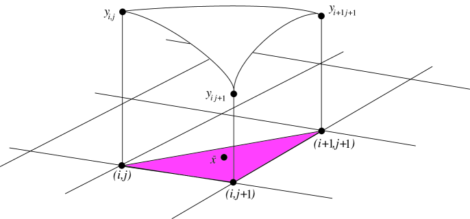
Figure 5.1: Depiction of the heuristic interpretation of an element of $J^{1}Y$ when $X$ is discrete.

Multisymplectic phase space.

We define the first jet bundle of $Y$ to be

$$J^{1}Y \equiv \bigl{\{}(y_{ij},y_{i\,j+1},y_{i+1\,j+1})\bigm{|}(i,j)\in X,\;y_{ij},y_{i\,j+1},y_{i+1\,j+1}\in\mathcal{F}\bigr{\}}$$

$$\equiv X^{\Delta}\times\mathcal{F}^{3}.$$

Heuristically (see Figure (5.1)), $X$ corresponds to some grid of elements $x_{ij}$ in continuous spacetime, say $\tilde{X}$, and $\bigl{(}y_{ij},y_{i\,j+1},y_{i+1\,j+1}\bigr{)}\in J^{1}Y$ corresponds to $j^{1}\phi(\bar{x})$, where $\bar{x}$ is “inside” the triangle bounded by $x_{ij},x_{i\,j+1},x_{i+1\,j+1}$, and $\phi$ is some smooth section of $\tilde{X}\times\mathcal{F}$ interpolating the field values $y_{ij},y_{i\,j+1},y_{i+1\,j+1}$. The first jet extension of a section $\phi$ of $Y$ is the map $j^{1}\phi:X^{\Delta}\rightarrow J^{1}Y$ defined by

$$j^{1}\phi(\Delta)\equiv\bigl{(}\Delta,\phi(\Delta^{1}),\phi(\Delta^{2}),\phi(\Delta^{3})\bigr{)}.$$

Given a vector field $Z$ on $Y$, we denote its restriction to the fiber $Y_{ij}$ by $Z_{ij}$, and similarly for vector fields on $J^{1}Y$. The first jet extension of a vector field $Z$ on $Y$ is the vector field $j^{1}Z$ on $J^{1}Y$ defined by

$$j^{1}Z(y_{\Delta^{1}},y_{\Delta^{2}},y_{\Delta^{3}})\equiv\big{(}Z_{\Delta^{1}}(y_{\Delta^{1}}),Z_{\Delta^{2}}(y_{\Delta^{2}}),Z_{\Delta^{3}}(y_{\Delta^{3}})\bigr{)},$$

for any triangle $\Delta$.

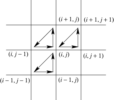
Figure 5.2: The triangles which touch $(i,j)$.

The variational principle.

Let us posit a discrete Lagrangian $L:J^{1}Y\rightarrow\mathbb{R}$. Given a triangle $\Delta$, define the function $L_{\Delta}:\mathcal{F}^{3}\rightarrow\mathbb{R}$ by

$$L_{\Delta}(y_{1},y_{2},y_{3})\equiv L(\Delta,y_{1},y_{2},y_{3}),$$

so that we may view the Lagrangian $L$ as being a choice of a function $L_{\Delta}$ for each triangle $\Delta$ of $X$. The variables on the domain of $L_{\Delta}$ will be labeled $y^{1},y^{2},y^{3}$, irrespective of the particular $\Delta$. Let $U$ be regular and let $\mathcal{C}_{U}$ be the set of sections of $Y$ on $U$, so $\mathcal{C}_{U}$ is the manifold $\mathcal{F}^{|U|}$. The action will assign real numbers to sections in $\mathcal{C}_{U}$ by the rule

$$S(\phi)\equiv\sum_{\Delta;\Delta\subseteq U}L\circ j^{1}\phi(\Delta).$$ (5.1)

Given $\phi\in\mathcal{C}_{U}$ and a vector field $V$, there is the 1-parameter family of sections

$$(F_{\epsilon}^{V}\phi)(i,j)\equiv F_{\epsilon}^{V_{ij}}(\phi(i,j)),$$

where $F^{V_{ij}}$ denotes the flow of $V_{ij}$ on $\mathcal{F}$. The variational principle is to seek those $\phi$ for which

$${\displaystyle\left.\frac{d}{d\epsilon}\right|_{\epsilon=0}}S(F_{\epsilon}^{V}\phi)=0$$

for all vector fields $V$.

The discrete Euler-Lagrange equations.

The variational principle gives certain field equations, the discrete Euler-Lagrange field equations (DELF equations), as follows. Focus upon some $(i,j)\in\operatorname{int}U$, and abuse notation by writing $\phi(i,j)\equiv y_{ij}$. The action, written with its summands containing $y_{ij}$ explicitly, is (see Figure (5.2))

$$S=\cdots+L(y_{ij},y_{i\,j+1},y_{i+1\,j+1})+L(y_{i\,j-1},y_{ij},y_{i+1\,j})+L(y_{i-1\,j-1},y_{i-1\,j},y_{ij})+\cdots$$

so by differentiating in $y_{ij}$, the DELF equations are

$$\frac{\partial L}{\partial y^{1}}(y_{ij},y_{i\,j+1},y_{i+1\,j+1})+\frac{\partial L}{\partial y^{2}}(y_{i\,j-1},y_{ij},y_{i+1\,j})+\frac{\partial L}{\partial y^{3}}(y_{i-1\,j-1},y_{i-1\,j},y_{ij})=0,$$

for all $(i,j)\in\operatorname{int}U$. Equivalently, these equations may be written

$$\sum_{l;\Delta;(i,j)=\Delta^{l}}\frac{\partial L_{\Delta}}{\partial y^{l}}(y_{\Delta^{1}},y_{\Delta^{2}},y_{\Delta^{3}})=0,$$ (5.2)

for all $(i,j)\in\operatorname{int}U$.

The discrete Cartan form.

Now suppose we allow nonzero variations on the boundary $\partial U$, so we consider the effect on $S$ of a vector field $V$ which does not necessarily vanish on $\partial U$. For each $(i,j)\in\partial U$ find the triangles in $U$ touching $(i,j)$. There is at least one such triangle since $(i,j)\in\operatorname{cl}U$; there are not three such triangles since $(i,j)\not\in\operatorname{int}U$. For each such triangle $\Delta$, $(i,j)$ occurs as the $l^{\mbox{\scriptsize th}}$ vertex, for one or two of $l=1,2,3$, and those $l^{\mbox{\scriptsize th}}$ expressions from the list

$$\displaystyle\frac{\partial L}{\partial y^{1}}(y_{ij},y_{i\,j+1},y_{i+1\,j+1})V_{ij}(y_{ij}),$$

$$\displaystyle\frac{\partial L}{\partial y^{2}}(y_{i\,j-1},y_{ij},y_{i+1\,j})V_{ij}(y_{ij}),$$

$$\displaystyle\frac{\partial L}{\partial y^{3}}(y_{i-1\,j-1},y_{i-1\,j},y_{ij})V_{ij}(y_{ij}),$$

yielding one or two numbers. The contribution to $dS$ from the boundary is the sum of all such numbers. To bring this into a recognizable format, we take our cue from discrete Lagrangian mechanics, which featured two $1$-forms. Here the above list suggests the three $1$-forms on $J^{1}Y$, the first of which we define to be

$$\Theta_{L}^{1}(y_{ij},y_{i\,j+1},y_{i+1\,j+1})\cdot(v_{y_{ij}},v_{y_{i\,j+1}},v_{y_{i+1\,j+1}})$$

$$\hskip 108.405pt\equiv\frac{\partial L}{\partial y^{1}}(y_{ij},y_{i\,j+1},y_{i+1\,j+1})\cdot(v_{y_{ij}},0,0),$$

$\Theta_{L}^{2}$ and $\Theta_{L}^{3}$ being defined analogously. With these notations, the contribution to $dS$ from the boundary can be written $\theta_{L}(\phi)\cdot V$, where $\theta_{L}$ is the $1$-form on the space of sections $\mathcal{C}_{U}$ defined by

$$\theta_{L}(\phi)\cdot V\equiv\sum_{\Delta;\Delta\cap\partial U\not=\emptyset}\left(\sum_{l;\Delta^{l}\in\partial U}\left[(j^{1}\phi)^{*}(j^{1}V\mathbin{\hbox to6.0pt{\vrule height=0.4pt,width=5.0pt,depth=0.0pt\kern-0.4pt\vrule height=6.0pt,width=0.4pt,depth=0.0pt\hss}}\Theta^{l}_{L})\right](\Delta)\right).$$ (5.3)

In comparing (5.3) with (4.56), the analogy with the multisymplectic formalism of Section (4) is immediate.

The discrete multisymplectic form formula.

Given a triangle $\Delta$ in $X$, we define the projection $\pi_{\Delta}:\mathcal{C}_{U}\rightarrow J^{1}Y$ by

$$\pi_{\Delta}(\phi)\equiv(\Delta,y_{\Delta^{1}},y_{\Delta^{2}},y_{\Delta^{3}}).$$

In this notation, it is easily verified that (5.3) takes the convenient form

$$\theta_{L}=\sum_{\Delta;\Delta\cap\partial U\not=\emptyset}\left(\sum_{l;\Delta^{l}\in\partial U}\pi_{\Delta}^{*}\Theta^{l}_{L}\right).$$ (5.4)

A first-variation at a solution $\phi$ of the DELF equations is a vertical vector field $V$ such that the associated flow $F^{V}$ maps $\phi$ to other solutions of the DELF equations. Set $\Omega^{l}_{L}=-d\Theta_{L}^{l}$. Since

$$\Theta_{L}^{1}+\Theta_{L}^{2}+\Theta_{L}^{3}=dL,$$ (5.5)

one obtains

$$\Omega_{L}^{1}+\Omega_{L}^{2}+\Omega_{L}^{3}=0,$$

so that only two of the three $2$-forms $\Omega_{L}^{l}$, $l=1,2,3$ are essentially distinct. Exactly as in Section (2), the equation $d^{2}S=0$, when specialized to two first-variations $V$ and $W$ now gives, by taking one exterior derivative of (5.4),

$$0=d\theta_{L}(\phi)(V,W)=\sum_{\Delta;\Delta\cap\partial U\not=\emptyset}\left(\sum_{l;\Delta^{l}\in\partial U}V\mathbin{\hbox to6.0pt{\vrule height=0.4pt,width=5.0pt,depth=0.0pt\kern-0.4pt\vrule height=6.0pt,width=0.4pt,depth=0.0pt\hss}}W\mathbin{\hbox to6.0pt{\vrule height=0.4pt,width=5.0pt,depth=0.0pt\kern-0.4pt\vrule height=6.0pt,width=0.4pt,depth=0.0pt\hss}}\pi_{\Delta}^{*}\Omega^{l}_{L}\right),$$

which in turn is equivalent to

$$\sum_{\Delta;\Delta\cap\partial U\not=\emptyset}\left(\sum_{l;\Delta^{l}\in\partial U}\left[(j^{1}\phi)^{*}(j^{1}V\mathbin{\hbox to6.0pt{\vrule height=0.4pt,width=5.0pt,depth=0.0pt\kern-0.4pt\vrule height=6.0pt,width=0.4pt,depth=0.0pt\hss}}j^{1}W\mathbin{\hbox to6.0pt{\vrule height=0.4pt,width=5.0pt,depth=0.0pt\kern-0.4pt\vrule height=6.0pt,width=0.4pt,depth=0.0pt\hss}}\Omega^{l}_{L})\right](\Delta)\right)=0.$$ (5.6)

Again, the analogy with the multisymplectic form formula for continuous spacetime (4.18) is immediate.

The discrete Noether theorem.

Suppose that a Lie group $G$ with Lie algera ${\mathfrak{g}}$ acts on $F$ by vertical symmetries in such a way that the Lagrangian $L$ is $G$-invariant. Then $G$ acts on $Y$ and $J^{1}Y$ in the obvious ways. Since there are three Lagrange $1$-forms, there are three momentum maps $J^{l}$, $l=1,2,3$, each one a $\mathfrak{g}^{*}$-valued function on triangles in $X$, and defined by

$$J^{l}_{\xi}\equiv\xi_{J^{1}Y}\mathbin{\hbox to6.0pt{\vrule height=0.4pt,width=5.0pt,depth=0.0pt\kern-0.4pt\vrule height=6.0pt,width=0.4pt,depth=0.0pt\hss}}\Theta_{L}^{l},$$

for any $\xi\in\mathfrak{g}$. Invariance of $L$ and (5.5) imply that

$$J^{1}+J^{2}+J^{3}=0,$$

so, as in the case of the $1$-forms, only two of the three momenta are essentially distinct. For any $\xi$, the infinitesimal generator $\xi_{Y}$ is a first-variation, so invariance of $S$, namely $\xi_{Y}\mathbin{\hbox to6.0pt{\vrule height=0.4pt,width=5.0pt,depth=0.0pt\kern-0.4pt\vrule height=6.0pt,width=0.4pt,depth=0.0pt\hss}}dS=0$ , becomes $\xi_{Y}\mathbin{\hbox to6.0pt{\vrule height=0.4pt,width=5.0pt,depth=0.0pt\kern-0.4pt\vrule height=6.0pt,width=0.4pt,depth=0.0pt\hss}}\theta_{L}=0$. By left insertion into (5.3), this becomes the discrete version of Noether’s theorem:

$$\sum_{\Delta;\Delta\cap\partial U\not=\emptyset}\left(\sum_{l;\Delta^{l}\in\partial U}J^{l}(\Delta)\right)=0.$$ (5.7)

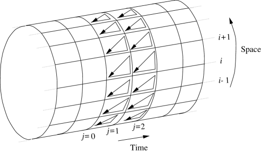
Figure 5.3: Symplectic flow and conservation of momentum from the discrete Noether theorem when the spatial boundary is empty and the temporal boundaries agree.

Conservation in a space and time split.

To understand the significance of (5.6) and (5.7) consider a discrete field theory with space a discrete version of the circle and time the real line, as depicted in Figure (5.3), where space is split into space and time, with “constant time” being constant $j$ and the “space index” $1\leq i\leq N$ being cyclic. Applying (5.7) to the region $\{(i,j)\mid j=0,1,2\}$ shown in the Figure, Noether’s theorem takes the conservation form

$$\sum_{i=1}^{N}J^{1}(y_{i0},y_{i1},y_{i+1\,1}) = -\sum_{i=1}^{N}\bigl{(}J^{2}(y_{i1},y_{i2},y_{i+1\,2})+J^{3}(y_{i1},y_{i2},y_{i+1\,2})\bigr{)}$$

$$= \sum_{i=1}^{N}J^{1}(y_{i1},y_{i2},y_{i+1\,2}).$$

Similarly, the discrete multisymplectic form formula also takes a conservation form. When there is spatial boundary, the discrete Noether theorem and the discrete multisymplectic form formulas automatically account for it, and thus form nontrivial generalizations of these conservation results.

Furthermore, as in the continuous case, we can achieve “evolution type” symplectic systems (i.e. discrete Moser-Veselov mechanical systems) if we define $Q$ as the space of fields at constant $j$, so $Q\equiv\mathcal{F}^{N}$, and take as the discrete Lagrangian

$$\tilde{L}([q_{j}^{0}],[q_{j}^{1}])\equiv\sum_{i=1}^{N}L(q_{i}^{0},q_{i}^{1},q_{i+1}^{1}).$$

Then the Moser-Veselov DEL evolution-type equations (3.2) are equivalent to the DELF equations (5.2), the multisymplectic form formula implies symplecticity of the Moser-Veselov evolution map, and conservation of momentum gives identical results in both the “field” and “evolution” pictures.

Example: nonlinear wave equation.

To illustrate the discretization method we have developed, let us consider the Lagrangian (4.32) of Section (4), which describes the nonlinear sine-Gordon wave equation. This is a completely integrable system with an extremely interesting hierarchy of soliton solutions, which we shall investigate by developing for it a variational multisymplectic-momentum integrator; see the recent article by Palais [1997] for a wonderful discussion on soliton theory.

To discretize the continuous Lagrangian, we visualize each triangle $\Delta$ as having base length $h$ and height $k$, and we think of the discrete jet $(y_{\Delta^{1}},y_{\Delta^{2}},y_{\Delta^{3}})$ as corresponding to the continuous jet

$$\frac{\partial\phi}{\partial x^{0}}(\bar{y}_{ij})=\frac{y_{i\,j+1}-y_{ij}}{h},\quad\frac{\partial\phi}{\partial x^{1}}(\bar{y}_{ij})=\frac{y_{i+1\,j+1}-y_{i\,j+1}}{k},$$

where $\bar{y}_{ij}$ is a the center of the triangle . This leads to the discrete Lagrangian

$$L=\frac{1}{2}\left(\frac{y_{2}-y_{1}}{h}\right)^{2}-\frac{1}{2}\left(\frac{y_{3}-y_{2}}{k}\right)^{2}+N\left(\frac{y_{1}+y_{2}+y_{3}}{3}\right),$$

with corresponding DELF equations

$$\frac{y_{{i+1\,j}}-2\,y_{{ij}}+y_{{i-1\,j}}}{{k}^{2}}-\frac{y_{{i\,j+1}}-2\,y_{{ij}}+y_{{i\,j-1}}}{{h}^{2}}$$ (5.8)

$$\qquad\mbox{}+\frac{1}{3}N^{\prime}\left(\frac{y_{{ij}}+y_{{i\,j+1}}+y_{{i+1\,j+1}}}{3}\right)$$

$$\qquad\qquad\mbox{}+\frac{1}{3}N^{\prime}\left(\frac{y_{{i\,j-1}}+y_{{ij}}+y_{{i+1\,j}}}{3}\right)$$

$$\qquad\qquad\qquad\mbox{}+\frac{1}{3}N^{\prime}\left(\frac{y_{{i-1\,j-1}}+y_{{i-1\,j}}+y_{{ij}}}{3}\right)=0.$$

When $N=0$ (wave equation) this gives the explicit method

$$y_{i\,j+1}=\frac{h^{2}}{k^{2}}(y_{{i+1\,j}}-2\,y_{{ij}}+y_{{i-1\,j}})+2\,y_{{ij}}-y_{{i\,j-1}},$$

which is stable whenever the Courant stability condition is satisfied.

Extensions: Jets from rectangles and other polygons.

Our choice of discrete jet bundle is obviously not restricted to triangles, and can be extended to rectangles or more general polygons (left of Figure( 5.4)). A rectangle is a quadruple of the form,

$$\Delta=\bigl{(}(i,j),(i,j+1),(i+1,j+1),(i+1,j)\bigr{)},$$

a point is an interior point of a subset $U$ of rectangles if $U$ contains all four rectangles touching that point, the discrete Lagrangian depends on variables $y_{1},\cdots,y_{4}$, and the DELF equations become

$$\frac{\partial L}{\partial y^{1}}(y_{ij},y_{i\,j+1},y_{i+1\,j+1},y_{i+1\,j})+\frac{\partial L}{\partial y^{2}}(y_{i\,j-1},y_{ij},y_{i+1\,j},y_{i+1\,j-1})$$

$$\qquad\mbox{+}\frac{\partial L}{\partial y^{3}}(y_{i-1\,j-1},y_{i-1\,j},y_{ij},y_{i\,j-1})+\frac{\partial L}{\partial y^{4}}(y_{i-1\,j},y_{i-1\,j+1},y_{i\,j+1},y_{ij})=0.$$

The extension to polygons with even higher numbers of sides is straightforward; one example is illustrated on the right of Figure( 5.4).

       

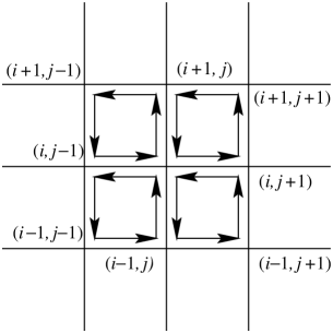
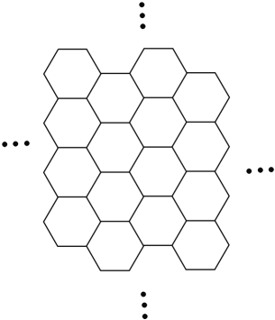
Figure 5.4: On the left, the method based on rectangles; on the right, a possible method based on hexagons.

The motivation for consideration of these extensions is enhancing the stability of the triangle-based method in the nonlinear wave example just above.

Example: nonlinear wave equation, rectangles.

Think of each rectangle $\Delta$ as having length $h$ and height $k$, and each discrete jet $(y_{\Delta^{1}},y_{\Delta^{2}},y_{\Delta^{3}},y_{\Delta^{4}})$ being associated to the continuous jet

$$\frac{\partial\phi}{\partial x^{0}}(p)=\frac{y_{i\,j+1}-y_{ij}}{h},\quad\frac{\partial\phi}{\partial x^{1}}(p)=\frac{1}{2}\left(\frac{y_{i+1\,j}-y_{i\,j}}{k}+\frac{y_{i+1\,j+1}-y_{i\,j+1}}{k}\right),$$

where $p$ is a the center of the rectangle. This leads to the discrete Lagrangian

$$L = \frac{1}{2}\left(\frac{y_{2}-y_{1}}{h}\right)^{2}-\frac{1}{2}\left(\frac{y_{4}-y_{1}}{2k}+\frac{y_{3}-y_{2}}{2k}\right)^{2}$$ (5.9)

$$\qquad\mbox{}+N\left(\frac{y_{1}+y_{2}+y_{3}+y_{4}}{4}\right).$$

If, for brevity, we set

$$\bar{y}_{ij}\equiv\frac{y_{ij}+y_{i\,j+1}+y_{i+1\,j+1}+y_{i+1\,j}}{4},$$

then one verifies that the DELF equations become

$$\Biggl{[}\frac{1}{2}\frac{y_{{i+1\,j}}-2\,y_{{ij}}+y_{{i-1\,j}}}{{k}^{2}}+\frac{1}{4}\frac{y_{{i+1\,j+1}}-2\,y_{{i\,j+1}}+y_{{i-1\,j+1}}}{{k}^{2}}$$

$$\qquad\mbox{}+\frac{1}{4}\frac{y_{{i+1\,j-1}}-2\,y_{{i\,j-1}}+y_{{i-1\,j-1}}}{{k}^{2}}\Biggr{]}-\Biggl{[}\frac{y_{{i\,j+1}}-2\,y_{{ij}}+y_{{i\,j-1}}}{{h}^{2}}\Biggr{]}$$

$$\qquad\qquad\mbox{}+\frac{1}{4}\Biggl{[}N^{\prime}(\bar{y}_{ij})+N^{\prime}(\bar{y}_{i\,j-1})+N^{\prime}(\bar{y}_{i-1\,j-1})+N^{\prime}(\bar{y}_{i-1\,j})\Biggr{]}=0,$$

which, if we make the definitions

$$\displaystyle\partial^{2}_{h}y_{ij}\equiv y_{{i\,j+1}}-2\,y_{{ij}}+y_{{i\,j-1}},\quad\partial^{2}_{k}y_{ij}\equiv y_{{i+1\,j}}-2\,y_{{ij}}+y_{{i-1\,j}},$$

$$\displaystyle\bar{N}^{\prime}(\bar{y}_{ij})\equiv\frac{1}{4}\Biggl{[}N^{\prime}(\bar{y}_{ij})+N^{\prime}(\bar{y}_{i\,j-1})+N^{\prime}(\bar{y}_{i-1\,j-1})+N^{\prime}(\bar{y}_{i-1\,j})\Biggr{]},$$

is (more compactly)

$$\frac{1}{k^{2}}\Biggl{[}\frac{1}{4}\partial^{2}_{k}y_{i\,j+1}+\frac{1}{2}\partial^{2}_{k}y_{ij}+\frac{1}{4}\partial^{2}_{k}y_{i\,j-1}\Biggr{]}-\frac{1}{h^{2}}\partial^{2}_{h}y_{ij}+\bar{N}^{\prime}(\bar{y}_{ij})=0.$$ (5.10)

These are implicit equations which must be solved for $y_{i\,j+1}$, $1\leq i\leq N$, given $y_{i\,j}$, $y_{i\,j-1}$, $1\leq i\leq N$; rearranging, an iterative form equivalent to (5.10) is

$$-\left(\frac{h^{2}}{2(h^{2}+2k^{2})}\right)y_{i+1\,j+1}+y_{i\,j+1}-\left(\frac{h^{2}}{2(h^{2}+2k^{2})}\right)y_{i-1\,j+1}$$

$$\qquad\mbox{}=\,\frac{h^{2}}{h^{2}+2k^{2}}\Bigl{(}(y_{{i+1\,j}}-2\,y_{{ij}}+y_{i-1\,j})$$

$$\qquad\qquad\qquad\qquad\mbox{}+\frac{1}{2}(y_{{i+1\,j-1}}-2\,y_{{i\,j-1}}+y_{{i-1\,j-1}})\Bigr{)}$$

$$\qquad\quad\mbox{}+\frac{2k^{2}}{h^{2}+2k^{2}}\left(2\,y_{{ij}}-y_{{i\,j-1}}\right)$$

$$\qquad\quad\mbox{}+\frac{h^{2}k^{2}}{2(h^{2}+2k^{2})}\bigl{(}N^{\prime}(\bar{y}_{ij})+N^{\prime}(\bar{y}_{i\,j-1})+N^{\prime}(\bar{y}_{i-1\,j-1})+N^{\prime}(\bar{y}_{i-1\,j})\bigr{)}.$$

In the case of the sine-Gordon equation the values of the field ought to be considered as lying in ${\mathbb{S}}^{1}$, by virtue of the vertical symmetry $y\mapsto y+2\pi$. Soliton solutions for example will have a jump of $2\pi$ and the method will fail unless field values at close-together spacetime points are differenced modulo $2\pi$. As a result it becomes important to calculate using integral multiples of small field-dependent quantities, so that it is clear when to discard multiples of $2\pi$, and for this the above iterative form is inconvenient. But if we define

$$\partial^{1}_{h}y_{ij}\equiv y_{{i\,j+1}}-\,y_{{ij}},\qquad\partial^{1}_{k}y_{ij}\equiv y_{{i+1\,j}}-\,y_{{ij}},$$

then there is the following iterative form, again equivalent to (5.10)

$$y_{i\,j+1}=y_{ij}+\partial^{1}_{h}y_{i\,j},\quad\mbox{and}$$

$$-\left(\frac{h^{2}}{2(h^{2}+2k^{2})}\right)\partial^{1}_{h}y_{i+1\,j}+\partial^{1}_{h}y_{i\,j}-\left(\frac{h^{2}}{2(h^{2}+2k^{2})}\right)\partial^{1}_{h}y_{i-1\,j}$$

$$\qquad\mbox{}=\,\frac{h^{2}}{h^{2}+2k^{2}}(3\partial^{2}_{k}y_{ij}+\partial^{2}_{k}y_{i\,j-1})+\frac{2k^{2}}{h^{2}+2k^{2}}\partial^{1}_{h}y_{ij}$$

$$\qquad\qquad\mbox{}+\frac{h^{2}k^{2}}{2(h^{2}+2k^{2})}\bar{N}^{\prime}(\bar{y}_{ij}).$$ (5.11)

One can also modify (5.9) so as to treat space and time symmetrically, which leads to the discrete Lagrangian

$$L = \frac{1}{2}\left(\frac{y_{2}-y_{1}}{2h}+\frac{y_{3}-y_{4}}{2h}\right)^{2}-\frac{1}{2}\left(\frac{y_{4}-y_{1}}{2k}+\frac{y_{3}-y_{2}}{2k}\right)^{2}$$

$$\qquad+N\left(\frac{y_{1}+y_{2}+y_{3}+y_{4}}{4}\right),$$

and one verifies that the DELF equations become

$$\frac{1}{k^{2}}\biggl{[}\frac{1}{4}\partial^{2}_{k}y_{i\,j+1}+\frac{1}{2}\partial^{2}_{k}y_{ij}+\frac{1}{4}\partial^{2}_{k}y_{i\,j-1}\biggr{]}$$

$$\qquad\mbox{}-\frac{1}{h^{2}}\biggl{[}\frac{1}{4}\partial^{2}_{h}y_{i+1\,j}+\frac{1}{2}\partial^{2}_{h}y_{ij}+\frac{1}{4}\partial^{2}_{h}y_{i-1\,j}\biggr{]}+\bar{N}^{\prime}(\bar{y}_{ij})=0,$$ (5.12)

an equivalent iterative form of which is

$$y_{i\,j+1}=y_{ij}+\partial^{1}_{h}y_{i\,j},\quad\mbox{and}$$

$$-\left(\frac{h^{2}-k^{2}}{2(h^{2}+k^{2})}\right)\partial^{1}_{h}y_{i+1\,j}+\partial^{1}_{h}y_{i\,j}-\left(\frac{h^{2}-k^{2}}{2(h^{2}+k^{2})}\right)\partial^{1}_{h}y_{i-1\,j}$$

$$\qquad\mbox{}=\,\frac{h^{2}}{2(h^{2}+k^{2})}(3\partial^{2}_{k}y_{ij}+\partial^{2}_{k}y_{i\,j-1})$$

$$\qquad\qquad\mbox{}+\frac{h^{2}}{2(h^{2}+k^{2})}(2\partial^{1}_{h}y_{ij}+\partial^{1}_{h}y_{i+1\,j}+\partial^{1}_{h}y_{i-1\,j})$$

$$\qquad\qquad\qquad\mbox{}+\frac{h^{2}k^{2}}{2(h^{2}+k^{2})}\bar{N}^{\prime}(\bar{y}_{ij}).$$ (5.13)

5.2 Numerical checks.

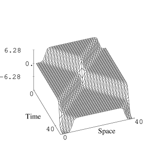
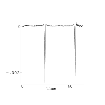
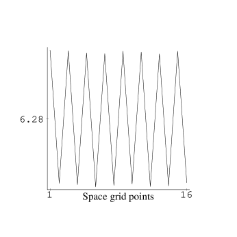
Figure 5.5: Top left: the wave forms for a two soliton kink and antikink collision using (5.12). Top right: the energy error. Bottom left: the wave form at time $t\approx 11855$. Bottom right: the portion of the bottom left graph for spatial grid points $1\ldots 16$.

While the focus of this article is not the numerical implementation of the integrators which we have derived, we have, nevertheless, undertaken some preliminary numerical investigations of our multisymplectic methods in the context of the sine-Gordon equation with periodic boundary conditions.

The rectangle-based multisymplectic method.

The top half of Figure (5.5) shows a simulation of the collision of “kink” and “antikink” solitons for the sine-Gordon equation, using the rectangle-based multisymplectic method (5.12). In the bottom half of that figure we show the result of running that simulation until the solitons have undergone about $460$ collisions; shortly after this the simulation stops because the iteration (5.13) diverges. The anomalous spatial variations in the waveform of the bottom left of Figure (5.5) have period $2$ spatial grid divisions and are shown in finer scale on the bottom right of that figure. These variations are reminiscent of those found in Ablowitz, Herbst and Schober [1996] for the completely integrable discretization of Hirota, where the variations are attributed to independent evolution of waveforms supported on even vs. odd grid points. Observation of (5.12) indicates what is wrong: the nonlinear term $N$ contributes to (5.12) in a way that will average out these variations, and consequently, once they have begun, (5.12) tends to continue such variations via the linear wave equation. In Ablowitz et. al., the situation is rectified when the number of spatial grid points is not even, and this is the case for (5.12) as well. This is indicated on the left of Figure (5.6), which shows the waveform after about $5000$ soliton collisions when $N=255$ rather than $N=256$. Figure (5.7) summarizes the evolution of energy error for that simulation.

Initial data.

For the two-soliton-collision simulations, we used the following initial data: $h=k/8$ (except $h=k/16$ where noted), where $k=40/N$ and $N=255$ spatial grid points (except Figure (5.5) where $N=256$). The circle that is space should be visualized as having circumference $L=40$. Let $\kappa=1-\epsilon$ where $\epsilon=10^{-6}$, $\tilde{L}=L/4=10$,

$$P=2\int_{0}^{1/\kappa}\!\!\!\!\frac{1}{\sqrt{1-y^{2}}\sqrt{1-\kappa^{2}y^{2}}}\,dy\approx 15.90,\qquad c=\sqrt{1-\frac{\tilde{L}^{2}}{\kappa^{2}P^{2}}}\approx.7773,$$

and

$$\tilde{\phi}(x)\equiv 2\arcsin\left(\operatorname{sn}\left(\frac{x}{\kappa\sqrt{1-c^{2}}};\kappa\right)\right).$$

Then $\tilde{\phi}(x-ct)$ is a kink solution if space has a circumference of $\tilde{L}$. This kink and an oppositely moving antikink (but placed on the last quarter of space) made up the initial field, so that $y_{i0}=\phi(40(i-1)/N)$, $i=1,\ldots,N$, where

$$\phi(x)\equiv\left\{\begin{array}[]{ll}\phi(x)&0\leq x<L/4\\ 2\pi&L/4\leq x<3L/4\\ 2\pi-\phi(x-3L/4)&3L/4\leq x<L\end{array}\right.,$$

while $y_{i1}=y_{i0}+\dot{\phi}(40(i-1)/N)h$ where

$$\dot{\phi}(x)\equiv\left\{\begin{array}[]{ll}(\phi(x-hc)-\phi(x))/h&0\leq x<L/4\\ 0&L/4\leq x<3L/4\\ -(\phi(x-hc)-\phi(x))/h&3L/4\leq x<L\end{array}\right..$$

Figure 5.6: On the left, the final wave form (after about 5000 soliton collisions at $t\approx 129133$) obtained using the rectangle-based multisymplectic method (5.12). On the right, the final waveform (at $t\approx 129145$) from the energy-conserving method (5.14) of Vu-Quoq and Li. In both simulations, temporal drift is occurring. For this reason the waveforms are inverted with respect to one another; moreover, the separate solitons are drifting at slightly different rates, as indicated by the off-center waveforms.

Figure 5.7: On the left, the energy error corresponding to our multisymplectic method (5.13) for 5000 solition collisions; the three graphs correspond to the minimum, average, and maximum energy error over consecutive 5000 time step regions. On the right, the final energy error (i.e. the energy error after about 5000 soliton collisions), which can be compared with the initial energy error plot in the top left of Figure (5.5).

Comparison with energy-conserving methods.

As an example of how our method compares with an existing method, we considered the energy-conserving method of Vu-Quoc and Li [1993], page 354:

$$\frac{1}{k^{2}}\biggl{[}\frac{1}{4}\partial^{2}_{k}y_{i\,j+1}+\frac{1}{2}\partial^{2}_{k}y_{ij}+\frac{1}{4}\partial^{2}_{k}y_{i\,j-1}\biggr{]}-\frac{1}{h^{2}}\partial^{2}_{h}y_{ij}$$

$$\qquad\mbox{}+\frac{1}{2}\left(\frac{N(y_{i\,j+1})-N(y_{ij})}{y_{i\,j+1}-y_{ij}}+\frac{N(y_{ij})-N(y_{i\,j-1})}{y_{ij}-y_{i\,j-1}}\right)=0.$$ (5.14)

This has an iterative form similar to (5.13) and is quite comparable with (5.10) and (5.12) in terms of the computation required. Our method seems to preserve the soliton waveform better than (5.14), as is indicated by comparison of the left and right Figure (5.6).

In regards to the closely related papers Vu-Quoc and Li [1993] and Li and Vu-Quoc [1995], we could not verify in our simulations that their method conserves energy, nor could we verify their proof that their method conserves energy. So, as a further check, we implemented the following energy-conserving method of Guo, Pascual, Rodriguez, and Vazquez [1986]:

$$\partial^{2}_{k}y_{ij}-\partial^{2}_{h}y_{ij}+\frac{N(y_{i\,j+1})-N(y_{i\,j-1})}{y_{i\,j+1}-y_{i\,j-1}},$$ (5.15)

which conserves the discrete energy

$$\sum_{j=1}^{N}\left(\frac{1}{2}\frac{(y_{i\,j+1}-y_{ij})(y_{ij}-y_{i\,j-1})}{h^{2}}+\frac{1}{2}\left(\frac{y_{i+1\,j}-y_{ij}}{k}\right)^{2}-N(y_{ij})\right).$$

This method diverged after just 345 soliton collisions.

Figure 5.8: A long-time simulation using the energy-conserving method (5.15) of Guo et al. Above left: the initial energy error. Above right: the average energy error over consecutive 5000 time step regions (the maximum and minimum closely parallel the average). Below left: the final energy error. Below right: the final waveform at $t\approx 129149$.

As can be seen from (5.15), the nonlinear potential $N$ enters as a difference over two grid spacings, which suggests that halving the time step might result in a more fair comparison with the methods (5.12) or (5.14). With this advantage, method (5.15) was able to simulate 5000 soliton collisions, with a waveform degradation similar to the energy-conserving method (5.14), as shown at the bottom right of Figure (5.8). The same figure also shows that, although the energy behavior of (5.15) is excellent for short time simulations, it drifts significantly over long times, and the final energy error has a peculiar appearance. Figure (5.9) shows the time evolution of the waveform through the soliton collision that occurs just before the simulation stops. Apparently, at the soliton collisions, significant high frequency oscillations are present, and these are causing the jumps in the energy error in the bottom left plot of Figure (5.8). This error then accumulates due to the energy-conserving property of the method. In these simulations, so as to guard against the possibility that this behavior of the energy was due to inadequately solving the implicit equation (5.15), we imposed a minimum limit of 3 iterations in the corresponding iterative loop, whereas this loop would otherwise have converged after just 1 iteration.

Figure 5.9: The soliton collision at time $t\approx 129130$, after the energy-conserving method (5.15) of Guo et al. has simulated about 5000 soliton collisions. The solitons collide beginning at the top left and proceed to the top right, then to the bottom left, and finally to the bottom right. The vertical scales are not constant and visually exaggerate the high frequency oscillations, which are small on the scale $0$ to $2\pi$.

Figure 5.10: Similar to the above plot but for our triangle-based multisymplectic method (5.8).

Comparison with the triangle-based multisymplectic method.

The discrete second derivatives in the method (5.15) are the same as in the triangle-based multisymplectic method (5.8); these derivatives are simpler than either our rectangle-based multisymplectic method (5.12) or the energy-conserving method of Vu-Quoc and Li (5.14). To explore this we implemented the triangle-based multisymplectic method (5.8). Even with the less complicated discrete second derivatives our triangle-based multisymplectic method simulated 5000 soliton collisions with comparable energy and waveform preservation properties as the rectangle-based multisymplectic method (5.12), as shown in Figure (5.11). Figure (5.10) shows the time evolution of the waveform through the soliton collision just before the simulation stops, and may be compared to Figure (5.9). As can be seen, the high frequency oscillations that are present during the soliton collisions are smaller and more smooth for the triangle-based multisymplectic method than for the energy-conserving method (5.15). A similar statement is true irrespective which of the two multisymplectic or two energy conserving methods we tested, and is true all along the waveform, irrespective of whether or not a soliton collision is occurring.

Figure 5.11: A simulation of 5000 soliton collisions using the triangle-based multisymplectic method (5.8). Above left: The initial energy error. Above right: The minimum, average and maximum energy as in the left of Figure (5.7). Below left: the final waveform (at $t\approx 129130$). Below right: the final energy error.

Summary.

Our multisymplectic methods are finite difference methods that are computationally competitive with existing finite difference methods. Our methods show promise for long-time simulations of conservative partial differential equations, in that, for long-time simulations of the sine-Gordon equation, our method 1) had superior energy-conserving behavior, even when compared with energy-conserving methods; 2) better preserved the waveform than energy-conserving methods; and 3) exhibited superior stability, in that our methods excited smaller and more smooth high frequency oscillations than energy-conserving methods. However, further numerical investigation is certainly necessary to make any lasting conclusions about the long-time behavior of our integrator.

The programs.

The programs that were used in the preceding simulations are “C” language implementations of the various methods. A simple tridiagonal LUD method was used to solve the linear equations (e.g. the left side of (5.13)), as in Vu-Quoc and Li [1993], page 379. An $8^{\mbox{\scriptsize th}}$ order extrapolator was used to provide a seed for the implicit step. All calculations were performed in double precision while the implicit step was terminated when the fields ceased to change to single precision; the program’s output was in single precision. The extrapolation usually provided a seed accurate enough so that the methods became practically explicit, in that for many of the time-steps the first or second run through the iterative loops solving the implicit equations solved those equations to single precision. However, in the absence of a regular spacetime grid the expenses of the extrapolation and solving the linear equation would grow. Our programs are freely available at URL http://www.cds.caltech.edu/cds.

6 Concluding Remarks

Here we make a few miscellaneous comments and remark on some work planned for the future.

Lagrangian reduction.

As mentioned in the text, it is useful to have a discrete counterpart to the Lagrangian reduction of Marsden and Scheurle [1993a,b], Holm, Marsden and Ratiu [1998a] and Cendra, Marsden and Ratiu [1998]. We sketch briefly how this theory might proceed. This reduction can be done for both the case of “particle mechanics” and for field theory.

For particle mechanics, the simplest case to start with is an invariant (say left) Lagrangian on the tangent bundle of a Lie group: $L:TG\rightarrow\mathbb{R}$. The reduced Lagrangian is $l:\mathfrak{g}\rightarrow\mathbb{R}$ and the corresponding Euler–Poincaré equations have a variational principle of Lagrange d’Alembert type in that there are constraints on the allowed variations. This situation is described in Marsden and Ratiu [1994].

The discrete analogue of this would be to replace a discrete Lagrangian $\mathbb{L}:G\times G\rightarrow\mathbb{R}$ by a reduced discrete Lagrangian $\ell:G\rightarrow\mathbb{R}$ related to $\mathbb{L}$ by

$$\ell(g_{1}g_{2}^{-1})=\mathbb{L}(g_{1},g_{2})$$

In this situation, the algorithm from $G\times G$ to $G\times G$ reduces to one from $G$ to $G$ and it is generated by $\ell$ in a way that is similar to that for $\mathbb{L}$. In addition, the discrete variational principle for $\mathbb{L}$ which states that one should find critical points of

$$\mathbb{L}(g_{1},g_{2})+\mathbb{L}(g_{2},g_{3})$$

with respect to $g_{2}$ to implicitly define the map $(g_{1},g_{2})\mapsto(g_{2},g_{3})$, reduces naturally to the following principle: Find critical points of $\ell(g)+\ell(h)$ with respect to variations of $g$ and $h$ of the form $g\xi:=L_{g}\xi$ and $\xi h=R_{h}\xi$ where $L_{g}$ and $R_{h}$ denote left and right translation and where $\xi\in\mathfrak{g}$. In other words, one sets to zero, the derivative of the sum $\ell(gg_{\epsilon}^{-1})+\ell(g_{\epsilon}h)$ with respect to $\epsilon$ at $\epsilon=0$ for a curve $g_{\epsilon}$ in $G$ that passes through the identity at $\epsilon=0$. This defines (with caveats of regularity as before) a map of $G$ to itself, which is the reduced algorithm. This algorithm can then be used to advance points in $G\times G$ itself, by advancing each component equally, reproducing the algorithm on $G\times G$. In addition, this can be used with the adjoint or coadjoint action to advance points in $\mathfrak{g}$ or $\mathfrak{g}^{\ast}$ to approximate the Euler–Poincaré or Lie–Poisson dynamics.

These equations for a discrete map, say $\phi_{\ell}:G\rightarrow G$ generated by $\ell$ on $G$ are called the discrete Euler–Poincaré equations as they are the discrete analogue of the Euler–Poincaré equations on $\mathfrak{g}$. Notice that, at least in theory, computation can be done for this map first and then the dynamics on $G\times G$ is easily reconstructed by simply advancing each pair as follows: $(g_{1},g_{2})\mapsto(hg_{1},hg_{2})$, where $h=\phi_{\ell}(g_{1}^{-1}g_{2})$.

If one identifies the discrete Lagrangians with generating functions (as explained in Wendlandt and Marsden [1997]) then the reduced Lagrangian generates the reduced algorithm in the sense of Ge and Marsden [1988], and this in turn is closely related to the Lie–Poisson–Hamilton–Jacobi theory.

Next, consider the more general case of $TQ$ with its discretization $Q\times Q$ with a group action (assumed to be free and proper) by a Lie group $G$. The reduction of $TQ$ by the action of $G$ is $TQ/G$, which is a bundle over $T(Q/G)$ with fiber isomorphic to $\mathfrak{g}$. The discrete analogue of this is $(Q\times Q)/G$ which is a bundle over $(Q/G)\times(Q/G)$ with fiber isomorphic to $G$ itself. The projection map $\pi:(Q\times Q)/G\rightarrow(Q/G)\times(Q/G)$ is given by $[(q_{1},q_{2})]\mapsto([q_{1}],[q_{2}])$ where $[\;]$ denotes the relevant equivalence class. Notice that in the case in which $Q=G$ this bundle is “all fiber”. The reduced discrete Euler-Lagrange equations are similar to those in the continuous case, in which one has shape equations couples with a version of the discrete Euler–Poincaré equations.

Of course all of the machinery in the continuous case can be contemplated here too, such as stability theory, geometric phases, etc. In addition, it would be useful to generalize this Lagrangian reduction theory to the multisymplectic case. All of these topics are planned for other papers.

Role of uniformity of the grid.

Consider an autonomous, continuous Lagrangian $\mathcal{L}:TQ\rightarrow\mathbb{R}$ where, for simplicity, $Q$ is an open submanifold of Euclidean space. Imagine some not necessarily uniform temporal grid ($t_{0},t_{1},\cdots$) of $\mathbb{R}$, so that $t_{0}<t_{1}<t_{2}<\cdots$. In this situation, it is natural to consider the discrete action

$$S=\sum_{k=1}^{n}L_{k}(q_{k},q_{k-1})\equiv\sum_{k=1}^{n}\mathcal{L}\left(\frac{q_{k}+q_{k-1}}{2},\frac{q_{k}-q_{k-1}}{t_{k}-t_{k-1}}\right)(t_{k}-t_{k-1}).$$ (6.1)

This action principle deviates from the action principle (3.1) of Section 3 in that the discrete Lagrangian density depends explicitly on $k$. Of course nonautonomous continuous Lagrangians also yield $k$-dependent discrete Lagrangian densities, irrespective of uniformity of the grid. Thus, nonuniform temporal grids or nonautonomous Lagrangians give rise to discrete Lagrangian densities which are more general those those we have considered in Section (3). For field theories, the Lagrangian in the action (5.1) depends on the spacetime variables already, through its explicit dependence on the triangle $\Delta$. However, it is only in the context of a uniform grid that we have experimented numerically and only in that context that we have discussed the significance of the discrete multisymplectic form formula and the discrete Noether theorem.

Using (6.1) as an example, will now indicate why the issue of grid uniformity may not be serious. The DEL equations corresponding to the action (6.1) are

$$\frac{\partial L_{k}}{\partial q_{1}}(q_{k},q_{k-1})+\frac{\partial L_{k+1}}{\partial q_{2}}(q_{k+1},q_{k})=0,\quad k=1,2,,\cdots,$$ (6.2)

and this gives evolution maps $F_{k+1,k}:Q\times Q\rightarrow Q\times Q$ defined so that

$$F_{k+1,k}(q_{k},q_{k-1})=(q_{k+1},q_{k}),\quad k=1,2,\cdots$$

when (6.2) holds. For the canonical 1-forms corresponding to (3.4) and (3.5) we have the $k$-dependent one forms

$$\theta_{L,k}^{-}(q_{1},q_{0})\cdot(\delta q_{1},\delta q_{0})\equiv\frac{\partial L_{k}}{\partial q_{0}}(q_{1},q_{0})\delta q_{0},$$ (6.3)

and

$$\theta_{L,k}^{+}(q_{1},q_{0})\cdot(\delta q_{1},\delta q_{0})\equiv\frac{\partial L_{k}}{\partial q_{1}}(q_{1},q_{0})\delta q_{1},$$ (6.4)

and Equations (3.7) and (3.9) become

$$F_{k+1,k}^{*}(d\theta_{L,k}^{+})=-d\theta_{L,k+1}^{-},\quad d\theta_{L,k}^{-}+d\theta_{L,k}^{+}=0$$ (6.5)

respectively. Together, these two equations give

$$F_{k+1,k}^{*}(d\theta_{L,k}^{+})=d\theta_{L,k+1}^{+},$$ (6.6)

and if we set

$$F_{k}\equiv F_{k,k-1}\circ F_{k-1,k-2}\circ\cdots\circ F_{2,1}$$

then  (6.6) chain together to imply $F_{k}^{*}(d\theta_{L,1}^{+})=d\theta_{L,k}^{+}$. This appears less than adequate since it merely says that the pull back by the evolution of a certain 2-form is, in general, a different 2-form. The significant point to note, however, is that this situation may be repaired at any $k$ simply by choosing $L_{k}=L_{1}$. It is easily verified that the analogous statement is true with respect to momentum preservation via the discrete Noether theorem.

Specifically, imagine integrating a symmetric autonomous mechanical system in a timestep adaptive way with Equations (6.2). As the integration proceeds, various timesteps are chosen, and if momentum is monitored it will show a dependence on those choices. A momentum-preserving symplectic simulation may be obtained by simply choosing the last timestep to be of equal duration to the first. This is the highly desirable situation which gives us some confidence that grid uniformity is a nonissue. There is one caveat: symplectic integration algorithms are evolutions which are high frequency perturbations of the actual system, the frequency being the inverse of the timestep, which is generally far smaller than the time scale of any process in the simulation. However, timestep adaptation schemes will make choices on a much larger time scale than the timestep itself, and then drift in the energy will appear on this larger time scale. A meaningful long-time simulation cannot be expected in the unfortunate case that the timestep adaptation makes repeated choices in a way that resonates with some process of the system being simulated.

The sphere.

The sphere cannot be generally uniformly subdivided into spherical triangles; however, a good approximately uniform grid is obtained as follows: start from an inscribed icosahedron which produces a uniform subdivision into twenty spherical isosceles triangles; these are further subdivided by halving their sides and joining the resulting points by short geodesics.

Elliptic PDEs.

The variational approach we have developed allows us to examine the multisymplectic structure of elliptic boundary value problems as well. For a given Lagrangian, we form the associated action function, and by computing its first variation, we obtain the unique multisymplectic form of the elliptic operator. The multisymplectic form formula contains information on how symplecticity interacts with spatial boundaries. In the case of two spatial dimensions, $X=\mathbb{R}^{2}$, $Y=\mathbb{R}^{3}$, we see that equation (4.51) gives us the conservation law

$$\text{div}{\mathcal{X}}=0,$$

where the vector ${\mathcal{X}}=(\omega^{0}(j^{1}V,j^{1}W),\omega^{1}(j^{1}V,j^{1}W))$.

Furthermore, using our generalized Noether theory, we may define momentum-mappings of the elliptic operator associated with its symmetries. It turns out that for important problems of spatial complexity arising in, for example, pattern formation systems, the covariant Noether current intrinsically contains the constrained toral variational principles whose solutions are the complex patterns (see Marsden and Shkoller [1997]).

There is an interesting connection between our variational construction of multisymplectic-momentum integrators and the finite element method (FEM) for elliptic boundary value problems. FEM is also a variationally derived numerical scheme, fundamentally differing from our approach in the following way: whereas we form a discrete action sum and compute its first variation to obtain the discrete Euler-Lagrange equations, in FEM, it is the original continuum action function which is used together with a projection of the fields and their variations onto appropriately chosen finite-dimensional spaces. One varies the projected fields and integrates such variations over the spatial domain to recover the discrete equations. In general, the two discretization schemes do not agree, but for certain classes of finite element bases with particular integral approximations, the resulting discrete equations match the discrete Euler-Lagrange equations obtained by our method, and are hence naturally multisymplectic.

To illustrate this concept, we consider the Gregory and Lin method of solving two-point boundary value problems in optimal control. In this scheme, the discrete equations are obtained using a finite element method with a basis of linear interpolants. Over each one-dimensional element, let $N_{1}$ and $N_{2}$ be the two linear interpolating functions. As usual, we define the action function by $S(q)=\int_{0}^{T}L(q(t),\dot{q}(t))dt$. Discretizing the interval $[0,T]$ into $N$$+$$1$ uniform elements, we may write the action with fields projected onto the linear basis as

$$S(q)=\sum_{k=0}^{N-1}\int_{k}^{k+1}L(\{N_{1}\phi_{k}+N_{2}\phi_{k+1}\},\{\dot{N}_{1}\phi_{k}+\dot{N}_{2}\phi_{k+1}\})dt.$$

Since the Euler-Lagrange equations are obtained by linearizing the action and hence the Lagrangian, and as the functions $N_{i}$ are linear, one may easily check that by evaluating the integrals in the linearized equations using a trapezoidal rule, the discrete Euler-Lagrange equations given in (3.3) are obtained. Thus, the Gregory and Lin method is actually a multisymplectic-momentum algorithm.

Applicability to fluid problems.

Fluid problems are not literally covered by the theory presented here because their symmetry groups (particle relabeling symmetries) are not vertical. A generalization is needed to cover this case and we propose to work out such a generalization in a future paper, along with numerical implementation, especially for geophysical fluid problems in which conservation laws such as conservation of enstrophy and Kelvin theorems more generally are quite important.

Other types of integrators.

It remains to link the approaches here with other types of integrators, such as volume preserving integrators (see, eg, Kang and Shang [1995], Quispel [1995]) and reversible integrators (see, eg, Stoffer [1995]). In particular since volume manifolds may be regarded as multisymplectic manifolds, it seems reasonable that there is an interesting link.

Constraints.

One of the very nice things about the Veselov construction is the way it handles constraints, both theoretically and numerically (see Wendlandt and Marsden [1997]). For field theories one would like to have a similar theory. For example, it is interesting that for fluids, the incompressibility constraint can be expressed as a pointwise constraint on the first jet of the particle placement field, namely that its Jacobian be unity. When viewed this way, it appears as a holonomic constraint and it should be amenable to the present approach. Under reduction by the particle relabeling group, such a constraint of course becomes the divergence free constraint and one would like to understand how these constraints behave under both reduction and discretization.

Acknowledgments

We would like to extend our gratitude to Darryl Holm, Tudor Ratiu and Jeff Wendlandt for their time, encouragement and invaluable input. Work of J. Marsden was supported by the California Institute of Technology and NSF grant DMS 96–33161. Work by G. Patrick was partially supported by NSERC grant OGP0105716 and that of S. Shkoller was partially supported by the Cecil and Ida M. Green Foundation and DOE. We also thank the Control and Dynamical Systems Department at Caltech for providing a valuable setting for part of this work.

References

Arms, J.M., J.E. Marsden, and V. Moncrief [1982] The structure of the space solutions of Einstein’s equations: II Several Killings fields and the Einstein-Yang-Mills equations. Ann. of Phys. 144, 81–106.

Ablowitz, M.J., Herbst, B.M., and C. Schober [1996] On the numerical solution of the Sine-Gordon equation 1. Integrable discretizations and homoclinic manifolds. J. Comp. Phys. 126, 299–314.

Abraham, R. and J.E. Marsden [1978] Foundations of Mechanics. Second Edition, Addison-Wesley.

Arms, J.M., J.E. Marsden, and V. Moncrief [1982] The structure of the space solutions of Einstein’s equations: II Several Killings fields and the Einstein-Yang-Mills equations. Ann. of Phys. 144, 81–106.

Arnold, V.I. [1978] Mathematical Methods of Classical Mechanics. Graduate Texts in Math. 60, Springer Verlag. (Second Edition, 1989).

Ben-Yu, G, P. J. Pascual, M. J. Rodriguez, and L. Vazquez [1986] Numerical solution of the sine-Gordon equation. Appl. Math. Comput. 18, 1–14

Bridges, T.J. [1997] Multi-symplectic structures and wave propagation. Math. Proc. Camb. Phil. Soc., 121, 147–190.

Calvo, M.P. and E. Hairer [1995] Accurate long-time integration of dynamical systems. Appl. Numer. Math., 18, 95.

Cendra, H., J. E. Marsden and T.S. Ratiu [1998] Lagrangian reduction by stages. preprint.

de Vogelaére, R. [1956] Methods of integration which preserve the contact transformation property of the Hamiltonian equations. Department of Mathematics, University of Notre Dame, Report No. 4.

Dragt, A.J. and J.M. Finn [1979] Normal form for mirror machine Hamiltonians, J. Math. Phys. 20, 2649–2660.

Ebin, D. and J. Marsden [1970] Groups of diffeomorphisms and the motion of an incompressible fluid. Ann. of Math. 92, 102-163.

Ge, Z. and J.E. Marsden [1988] Lie-Poisson integrators and Lie-Poisson Hamilton-Jacobi theory. Phys. Lett. A 133, 134–139.

Gotay, M., J. Isenberg, and J.E. Marsden [1997] Momentum Maps and the Hamiltonian Structure of Classical Relativistic Field Theories, I. Preprint.

Gregory, J and C. Lin [1991], The numerical solution of variable endpoint problems in the calculus of variations, Lecture Notes in Pure and Appl. Math., 127, 175–183.

Guo, B. Y., P. J. Pascual, M. J. Rodriguez, and L. Vazquez [1986] Numerical solution of the sine-Gordon equation. Appl. Math. Comput. 18, 1–14.

Holm, D. D., Marsden, J. E. and Ratiu, T. [1998a] The Euler-Poincaré equations and semidirect products with applications to continuum theories. Adv. in Math. (to appear).

Holm, D. D., J.E. Marsden and T. Ratiu [1998b] The Euler-Poincaré equations in geophysical fluid dynamics, in Proceedings of the Isaac Newton Institute Programme on the Mathematics of Atmospheric and Ocean Dynamics, Cambridge University Press (to appear).

Li, S. and L., Vu-Quoc [1995] Finite-difference calculus invariant structure of a class of algorithms for the nonlinear Klein-Gordon equation. SIAM J. Num. Anal. 32, 1839–1875.

Marsden, J.E., G.W. Patrick, and W.F. Shadwick (Eds.) [1996] Integration Algorithms and Classical Mechanics. Fields Institute Communications 10, Am. Math. Society.

Marsden, J.E. and T.S. Ratiu [1994] Introduction to Mechanics and Symmetry. Texts in Applied Mathematics 17, Springer-Verlag.

Marsden, J.E. and S. Shkoller [1997] Multisymplectic geometry, covariant Hamiltonians and water waves. To appear in Math. Proc. Camb. Phil. Soc. 124.

Marsden, J.E. and J.M. Wendlandt [1997] Mechanical systems with symmetry, variational principles and integration algorithms. Current and Future Directions in Applied Mathematics, Edited by M. Alber, B. Hu, and J. Rosenthal, Birkhäuser, 219–261.

McLachlan, R.I. and C. Scovel [1996] A survey of open problems in symplectic integration. Fields Institute Communications 10, 151–180.

Moser, J. and A.P. Veselov [1991] Discrete versions of some classical integrable systems and factorization of matrix polynomials. Comm. Math. Phys. 139, 217–243.

Neishtadt, A. [1984] The separation of motions in systems with rapidly rotating phase. P.M.M. USSR 48, 133–139.

Palais, R.S. [1968] Foundations of global nonlinear analysis, Benjamin, New York.

Palais, R.S. [1997] The symmetries of solitons. Bull. Amer. Math. Soc. 34, 339–403.

Quispel, G.R.W. [1995] Volume-preserving integrators. Phys. Lett. A. 206, 26.

Sanz-Serna, J. M. and M. Calvo [1994] Numerical Hamiltonian Problems. Chapman and Hall, London.

Simo, J.C.and O. Gonzalez. [1993], Assessment of Energy-Momentum and Symplectic Schemes for Stiff Dynamical Systems. Proc. ASME Winter Annual Meeting, New Orleans, Dec. 1993.

Stoffer, D. [1995] Variable steps for reversible integration methods, Computing 55, 1.

Veselov, A.P. [1988] Integrable discrete-time systems and difference operators. Funkts. Anal. Prilozhen. 22, 1–13.

Veselov, A.P. [1991] Integrable Lagrangian correspondences and the factorization of matrix polynomials. Funkts. Anal. Prilozhen. 25, 38–49.

Vu-Quoc, L. and S. Li [1993] Invariant-conserving finite difference algorithms for the nonlinear Klein-Gordon equation. Comput. Methods Appl. Mech. Engrg. 107, 341–391.

Wald, R.M. [1993] Variational principles, local symmetries and black hole entropy. Proc. Lanczos Centennary volume SIAM, 231–237.

Wendlandt, J.M. and J.E. Marsden [1997] Mechanical integrators derived from a discrete variational principle. Physica D 106, 223–246.