The Computational Complexity of Knot and Link Problems

Abstract

We consider the problem of deciding whether a polygonal knot in 3-dimensional Euclidean space is unknotted, capable of being continuously deformed without self-intersection so that it lies in a plane. We show that this problem, unknotting problem is in NP. We also consider the problem, unknotting problem of determining whether two or more such polygons can be split, or continuously deformed without self-intersection so that they occupy both sides of a plane without intersecting it. We show that it also is in NP. Finally, we show that the problem of determining the genus of a polygonal knot (a generalization of the problem of determining whether it is unknotted) is in PSPACE. We also give exponential worst-case running time bounds for deterministic algorithms to solve each of these problems. These algorithms are based on the use of normal surfaces and decision procedures due to W. Haken, with recent extensions by W. Jaco and J. L. Tollefson.

Keywords: knot theory, three-dimensional topology, computational complexity

1 Introduction

The problems dealt with in this paper might reasonably be called “computational topology”; that is, we study classical problems of topology (specifically, the topology of $1$-dimensional curves in $3$-dimensional space) with the objective of determining their computational complexity. One of the oldest and most fundamental of such problems is that of determining whether a closed curve embedded in space is unknotted (that is, whether it is capable of being continuously deformed without self-intersection so that it lies in a plane). Topologists study this problem at several levels, with varying meanings given to the terms “embedded” and “deformed”. The level that seems most appropriate for studying computational questions is that which topologists call piecewise-linear. At this level, a closed curve is embedded in space as a simple (non-self-intersecting) polygon with finitely many edges. Such an embedding is called a knot. (Operating at the piecewise-linear level excludes wild knots, such as those given by certain polygons with infinitely many edges which do not have nice neighborhoods or thickenings.) More generally, one may study links. A link is a finite collection of simple polygons disjointly embedded in 3-dimensional space. The individual polygons are called components of the link and a knot is a link with one component.

A continuous deformation is required to be piecewise-linear; that is, it consists of a finite number of stages, during each of which every vertex of the polygon moves linearly with time. From stage to stage the number of edges in the polygon may increase (by subdivision of edges at the beginning of a stage) or decrease (when cyclically consecutive edges become collinear at the end of a stage). If the polygon remains simple throughout this process, the deformation is called an isotopy between the initial and final knots. Knot isotopy defines an equivalence relation, called equivalence of knots. It is easy to see that all knots that lie in a single plane are equivalent; knots in this equivalence class are said to be unknotted or trivial knots.

We may remark at this point that while it is “intuitively clear” that there are non-trivial knots, it is not at all obvious how to prove this. Stillwell [37] traces the mathematical notion of knot back to a paper of A. T. Vandermonde in 1771; the first convincing proof of the non-triviality of a knot seems to be due to Max Dehn [8] in 1910.

There are a great many alternative formulations of the notion of knot equivalence. Here are some.

1. One can consider sequences of elementary moves, which are very simple isotopies that move a single edge across a triangle to the opposite two sides, or vice versa.

2. One can consider ambient isotopies that move not only the knot, but also the space in which it is embedded, in a piecewise-linear way.

3. One can consider homeomorphisms (continuous bijections that have continuous inverses) that map the space to itself in a piecewise-linear way, are orientation preserving, and send one knot to the other.

One can also study knots or links by looking at their projections onto a generic plane. In this way, a knot or link may be represented by a planar graph, called a knot diagram or link diagram, in which all vertices (representing the crossings of edges of the polygon) have degree four, and for which an indication is given at each crossing of which edge goes “over” and which edge goes “under”. This gives an additional formulation of equivalence:

1. One may consider sequences of Reidemeister moves, which are simple transformations on the diagram of a knot that leave the equivalence class of the knot unchanged.

For more details on piecewise-linear topology, the various formulations of knot and link equivalence, and many other aspects of knot theory, we recommend the books [1], [6], [30]. An introduction to the notions of complexity which we use can be found in [9],[41].

In order to study the computational complexity of knot and link problems, we must agree on a finite computational representation of a knot or link. There are two natural representations: a polygonal representation in 3-dimensional space, or a link diagram representing a 2-dimensional projection.

A polygonal representation of a link $L$ consists of a set of simple polygons in 3-dimensional space described by listing the vertices of each polygon in order; we assume that these vertices have rational coordinates. We can reduce to the case of integer lattice point vertices by replacing $L$ by a scaled multiple $mL$ for a suitable integer $m$. This does not change the equivalence class of $L$. A particularly simple kind of polygonal representation uses only integer lattice points as vertices and edges of unit length, so that the polygon is a closed self-avoiding walk on the integer lattice; a sequence of moves (up, down, north, south, east, west) that traverse the polygon, returning to the starting point without visiting any other point twice. (This formulation was used by Pippenger [27] and Sumners and Whittington [39] to show that “almost all” long self-avoiding polygons are non-trivially knotted.) The size of a polygonal representation $L$ is the number of edges in $L$; its input length is the number of bits needed to describe its vertices, in binary.

A link diagram ${\cal D}$ is a planar graph with some extra labeling for crossings that specifies a (general position) two-dimensional projection of a link. A precise definition is given in Section 3. The size of a link diagram is the number of vertices in $D$.

These two representations are polynomial-time equivalent in the following sense. Given a polygonal representation $L$ one can find in polynomial time in its input length a planar projection yielding a link diagram ${\cal D}$; if $L$ has $n$ edges then the graph ${\cal D}$ has at most $O(n^{2})$ vertices. Conversely given a link diagram ${\cal D}$ with $n$ vertices and $l$ components, one can compute in time polynomial in $n+l$ a polygonal link $L$ with $O(n+l)$ edges that has integer vertices and input length $O(n+l)$ and which projects in the $z$-direction onto the link diagram ${\cal D}$; see Section 7.

In this paper we consider knots and links as represented by link diagrams and take the crossing number as the measure of input size. We can now formulate the computational problem of recognizing unknotted polygons as follows:

Problem: UNKNOTTING PROBLEM
Instance: A link diagram ${\cal D}$.
Question:	Is ${\cal D}$ a knot diagram that represents the trivial knot?

See Welsh [41]—[43] for more information on this problem. The main result of this paper is the following.

Theorem 1.1

The unknotting problem is in NP.

The unknotting problem was shown to be decidable by Haken [10]; the result was announced in 1954, and the proof published in 1961. From then until now, we know of no strengthening of Haken’s decision procedure to give an explicit complexity bound. We present such a bound in Theorem 8.1.

We also study the splittability of links. A link is said to be splittable if it can be continuously deformed (by a piecewise-linear isotopy so that one or more curves of the link can be separated from one or more other curves by a plane that does not itself intersect any of the curves. We note that this notion remains unchanged if we replace “plane” by “sphere” in the definition. We formulate the computational problem of recognizing splittable links as follows.

Problem: SPLITTING PROBLEM

Instance: A link diagram ${\cal D}$.

Question: Is the link represented by ${\cal D}$ splittable?

The splitting problem was shown to be decidable by Haken [10] in 1961, see also Schubert [34]. We establish the following result.

Theorem 1.2

The splitting problem is in NP.

Another generalization of the unknotting problem concerns the genus $g(K)$ of a knot $K$. This is an integer assoicated to each knot, which is invariant under isotopy. It was defined by Seifert [36] in 1935; an informal account of the definition follows. Given a knot $K$, consider the class ${\cal S}(K)$ of all orientable spanning surfaces for $K$; that is, embedded orientable surfaces that have $K$ as their boundary. Seifert showed that this class is non-empty for any knot $K$. We assume in this discussion that all surfaces are triangulated and embedded in a piecewise-linear way. Up to piecewise-linear homeomorphism, an orientable surface is characterized by the number of boundary curves and the number of “handles”, which is called the genus of the surface. The genus $g(K)$ of the knot $K$ is defined to be the minimum genus of any surface in ${\cal S}(K)$. Seifert showed that a trivial knot $K$ is characterized by the condition $g(K)=0$. Since an orientable surface with one boundary curve and no handles is homeomorphic to a disk, this means that a knot is trivial if and only if it has a spanning disk.

The notion of genus gives us a natural generalization of the problem of recognizing unknotted polygons; we formulate the problem of computing the genus as a language-recognition problem in the usual way.

Problem: GENUS PROBLEM
Instance: A link diagram ${\cal D}$ and a natural number $k$.
Question:	Does the link diagram ${\cal D}$ represent a knot $K$ with $g(K)\leq k$?

Haken [10] also gave a decision procedure to determine the genus of a knot. We establish the following result.

Theorem 1.3

The genus problem is in PSPACE.

In 1961 Schubert [34] extended Haken’s methods to show the decidability of the genus problem on an arbitrary compact 3-manifold with boundary. (In this more general situation, it is necessary to first determine whether there exists any orientable surface which has the given embedded knot as boundary, and if so, determine the minimal genus.) Our analysis in principle extends to this case.

We also obtain exponential worst case running time bounds for deterministic algorithms to solve the above three problems. The input size $n$ is measured by the crossing measure of a link diagram. For the unknotting problem and the splitting problem these algorithms run in time $O(2^{cn})$ and space $O(n\log^{2}n)$ on a Turing machine. We show that the genus $g(K)$ for a knot $K$ presented as a knot diagram ${\cal K}$ can be computed in time $O(2^{cn^{2}})$ and space $O(n^{2})$, on a Turing machine.

The results in this paper were announced in the Proceedings of the 38th Annual Symposium on Foundations of Computer Science in Miami Florida in October, 1997 [13].

2 Historical Background

Recognizing whether two knots are equivalent has been one of the motivating problems of knot theory. A great deal of effort has been devoted to a quest for algorithms for recognizing the unknot, beginning with the work of Dehn [8] in 1910. Dehn’s idea was to look at the fundamental group of the complement of the knot, for which a finite presentation in terms of generators and relations can easily be obtained from a standard presentation of the knot. Dehn claimed that a knot is trivial if and only if the corresponding group is infinite cyclic. The proof of what is still known as “Dehn’s Lemma” had a gap, which remained until filled by Papakyriakopoulos in 1957 [26]. A consequence is the criterion that a curve is knotted if and only if the fundamental group of its complement is nonabelian. Dehn also posed the question of deciding whether a finitely presented group is isomorphic to the infinite cyclic group. During the 1950’s it was shown that many such decision problems for finitely presented groups, not necessarily arising from knots, are undecidable (see Rabin [28], for example), thus blocking this avenue of progress. The avenue has been traversed in the reverse direction, however: there are decision procedures for restricted classes of finitely presented groups arising from topology. In particular, computational results for properties of knots that are characterized by properties of the corresponding groups can be interpreted as computational results for knot groups.

Abstracting somewhat from Dehn’s program, we might try to recognize knot triviality by finding an invariant of the knot that (1) can be computed easily and (2) assumes some particular value only for the trivial knot. (Here invariant means invariant under isotopy.) Thus Alexander [2] defined in 1928 an invariant $A_{K}(x)$ (a polynomial in the indeterminate $x$) of the knot $K$ that can be computed in polynomial time. Unfortunately, it turns out that many non-trivial knots have Alexander polynomial $A_{K}(x)=1$, the same as the Alexander polynomial of the trivial knot.

Another invariant that has been investigated with the same hope is the Jones polynomial $J_{K}(x)$ of a knot $K$, discovered by Jones [22] in 1985. In this case the complexity bound is less attractive: the Jones polynomial for links (a generalization of the Jones polynomial for knots) is #P-hard and in ${\bf FP}^{\bf\#P}$ (see Jaeger, Vertigan and Welsh [21]). It is an open question whether trivial knots are characterized by their Jones polynomial. Even this prospect, however, has led Welsh [41] to observe that an affirmative answer to the last open question would yield an algorithm in ${\bf P}^{\bf\#P}$ for recognizing trivial knots, and to add: “By the standards of the existing algorithms, this would be a major advance.”

The revolution started by the Jones polynomial has led to the discovery of a great number of new knot and link invariants, including Vassiliev invariants and invariants associated to topological quantum field theories, see Birman [4] and Sawin [32]. The exact ability of these invariants to distinguish knot types has not been determined.

A different approach to the problems of recognizing unknottedness and deciding knot equivalence eventually led to decision procedures. This approach is based on the study of normal surfaces in 3-manifolds (defined in Section 3), which was initiated by Kneser [23] in 1929. In the 1950’s Haken developed the theory of normal surfaces, and obtained a decision procedure for unknottedness in 1961. Haken considered compact orientable 3-manifolds. Schubert [34] extended Haken’s procedure to decide the knot genus problem and related problems on arbitrary compact 3-manifolds with boundary. Haken also outlined an approach via normal surfaces to decide the knot equivalence problem [40]:

Problem: KNOT EQUIVALENCE PROBLEM
Instance: Two link diagrams ${{\mathcal{D}}}_{1}$ and ${{\mathcal{D}}}_{2}$.
Question:	Are ${{\mathcal{D}}}_{1}$ and ${{\mathcal{D}}}_{2}$ knot diagrams of equivalent knots?

The final step in this program was completed by Hemion [14] in 1979. This program actually solves a more general decision problem, concerning a large class of 3-manifolds, now called Haken manifolds, which can be cut into “simpler” pieces along certain surfaces (incompressible surfaces), eventually resulting in a collection of 3-balls. Knot complements are examples of Haken manifolds. It gives a procedure to decide if two Haken manifolds are homeomorphic [18]. Recent work of Jaco-Oertel [18] and Jaco-Tollefson [20] further simplified some of these algorithms.

Apart from these decidability results, there appear to be no explicit complexity bounds, either upper or lower, for any of the three problems that we study. The work of Haken [10] and Schubert [34] predates the currently used framework of complexity classes and hierarchies. Their algorithms were originally presented in a framework (handlebody decompositions) that makes complexity analysis difficult, but it was recognized at the time that implementation of their algorithms would require at least exponential time in the best case. More recently Jaco and others reformulated normal surface theory using piecewise linear topology, but did not determine complexity bounds. Other approaches to knot and link algorithms include methods related to Thurston’s geometrization program for 3-manifolds (see [11] for a survey) and methods based on encoding knots as braids (see Birman-Hirsch [5]). These approaches currently have unknown complexity bounds.

Our results are obtained using a version of normal surface theory as developed by Jaco-Rubinstein [19]. Among other things we show that Haken’s original approach yields an algorithm which determines if a knot diagram with $n$ crossings is unknotted in time $O(\exp(cn^{2}))$, and that the improved algorithm of Jaco-Tollefson runs in time $O(\exp(cn))$, see Theorem 8.1. The complexity class inclusions that we prove require some additional observations.

3 Knots and Links

A knot is an embedding $f:{\bf S}^{1}\to\mathbb{R}^{3}$, although it is usually identified with its image $K=f({\bf S}^{1})$; we are thus considering unoriented knots. A link with $k$ components is a collection of $k$ knots with disjoint images. An equivalent formulation regards a knot as an embedding in the one-point compactification ${\bf S}^{3}$ of ${\mathbb{R}^{3}}$, and we will sometimes use this setting.

Two knots $K$ and $K^{\prime}$ are ambient isotopic if there exists a homotopy $h_{t}:\mathbb{R}^{3}\to\mathbb{R}^{3}$ for $0\leq t\leq 1$ such that $h_{0}$ is the identity, each $h_{t}$ is a homeomorphism, and $h_{1}(K)=K^{\prime}$. We shall also say in this case that $K$ and $K^{\prime}$ are equivalent knots. Since we consider unoriented knots, we will also set two knots equivalent if they are equal after composing with a reflection of $S^{1}$. Our results work equally well for oriented or unoriented knots.

A knot or link is tame if it is ambient isotopic to a piecewise-linear knot or link, abbreviated as PL-knot or PL-link, and also called a polygonal knot or link. This paper considers PL-knots and links. Given this restriction, we can without further loss of generality restrict our attention to the piecewise-linear settings (see Moise [24]).

A regular projection of a knot or link is an orthogonal projection into a plane (say $z=0$) that contains only finitely many multiple points, each of which is a double point with transverse crossing. Any regular projection of a link gives a link diagram ${\mathcal{D}}$, which is an undirected labeled planar graph such that:

1. Connected components with no vertices are loops, simple closed curves disjoint from the rest of the diagram.

2. Each non-loop edge meets a vertex at each of its two ends (possibly the same vertex), and has a label at each end indicating an overcrossing or undercrossing at that end.

3. Each vertex has exactly four incident edges, two labeled as overcrossings and two labeled as undercrossings, and has a cyclic ordering of the incident edges that alternates overcrossings and undercrossings.

Conversely, every labeled planar graph satisfying these conditions is a link diagram for some link.

Given a link diagram, if we connect the edges across vertices according to the labeling, then the diagram separates into $k$ edge-connected components, where $k$ is the number of components in the link. A knot diagram is a link diagram having one component. A trivial knot diagram is a single loop with no vertices. It is straightforward to see that all knots with the same diagram are isotopic.

We define the crossing measure of a link diagram ${\mathcal{D}}$ to be the number of vertices in the diagram, plus the number of connected components in the diagram, minus one.

$$n=\#(\mbox{vertices of}~{}{\mathcal{L}})+\#(\mbox{connected components})-1~{}.$$ (1)

For knot diagrams, the crossing measure is equal to the crossing number, which is the number of vertices in the diagram. A trivial knot diagram is the only link diagram with crossing measure zero. All other link diagrams have strictly positive crossing measure.

A knot diagram is the unknot (or is unknotted) if there is a knot $K$ having this diagram that is ambient isotopic to a knot $K^{\prime}$ having a trivial knot diagram.

One can convert a knot diagram to any other diagram of an equivalent knot by a finite sequence of combinatorial transformations called Reidemeister moves. Reidemeister showed that a knot diagram ${\mathcal{K}}$ is unknotted if and only if there is a finite sequence of Reidemeister moves that convert it to the trivial knot diagram. In this sense the unknotting problem is a purely combinatorial problem, though with no obvious bound on the number of steps, see [12], [42].

4 Unknottedness Criterion

Our approach to solving the unknotting problem, based on that of Haken, relies on the following criterion for unknottedness: A PL-knot $K$ embedded in $\mathbb{R}^{3}$ is unknotted if and only if there exists a piecewise-linear disk $D$ embedded in $\mathbb{R}^{3}$ whose boundary $\partial D$ is the knot $K$ transversed once. We call such a disk $D$ a spanning disk. We shall actually use a weaker unknottedness criterion, given in Lemma 4.1 below. It does not deal with a spanning disk of $K$, but rather with a spanning disk of another knot $K^{\prime}$ which is ambient isotopic to $K$.

Given a PL-knot $K$, let ${\mathcal{T}}$ be a finite triangulation of ${\bf S}^{3}$ containing $K$ in its 1-skeleton, where the 3-sphere ${\bf S}^{3}$ is the one-point compactification of $\mathbb{R}^{3}$, and the point “at infinity” is a vertex of the triangulation. Barycentrically subdivide ${\mathcal{T}}$ twice to obtain a triangulation ${\mathcal{T}}^{\prime\prime}$, and let $M_{K}={\bf S}^{3}-R_{K}$ denote the compact triangulated 3-manifold with boundary obtained by deleting the open regular neighborhood $R_{K}$ of $K$. Here $R_{K}$ consists of all open simplices whose closure intersects $K$. The closure $\bar{R}_{K}$ of $R_{K}$ is a solid torus neighborhood of $K$, a solid torus containing $K$ as its central axis, and its boundary $\partial R_{K}=\partial M_{K}$ is homeomorphic to a 2-torus. See [15] for details of this construction. Each of $R_{K}$, $M_{K}$ and $\partial R_{K}=\partial M_{K}$ are triangulated by simplices in ${\mathcal{T}}^{\prime\prime}$. We call the manifold $M_{K}$ a knot complement manifold.

We call a triangulation of $M_{K}={\bf S}^{3}-R_{K}$ constructed as above a good triangulation of $M_{K}$. Similarly we define a good triangulation of a link complement manifold. For any good triangulation of $M_{K}$, the homology group $H_{1}(\partial M_{K};\mathbb{Z})\approx\mathbb{Z}\oplus\mathbb{Z}$, since $\partial M_{K}$ is a 2-torus. The kernel of the homology homomorphism induced by the inclusion map of $\partial M_{K}$ into $M_{K}$ is infinite cyclic (see Theorem 3.1 of [6] for a proof.) We take as generator $(1,0)$ the homology class of a fixed closed oriented simple closed curve which is the boundary $\partial B$ of an essential disk $B$ in $\overline{R}_{K}$ (a meridian) and as generator $(0,1)$ the homology class of a fixed closed oriented circle in $\partial M_{K}$ that has algebraic intersection $1$ with the meridian and algebraic linking number $0$ with $K$ (a longitude). A simple closed curve in $\partial\overline{R}_{K}$ whose homology class is trivial in the 3-manifold $\overline{R}_{K}$ but not in the surface $\partial\overline{R}_{K}$ is a meridian. A simple closed curve in $\partial R_{K}$ whose homology class is trivial in the 3-manifold $M_{K}$ but not in the surface $\partial\overline{R}_{K}$ is a longitude. The homology classes of a meridian and a longitude are well-defined up to orientation.

A compact surface $S$ with boundary $\partial S$ in a compact 3-manifold with boundary $(M,\partial M)$ is said to be properly embedded if it does not intersect itself and if $S\cap\partial M=\partial S$. A surface $S$ is essential in $M$ if it is properly embedded in $M$, cannot be homotoped into $\partial M$ while holding $\partial S$ fixed, and its fundamental group $\pi_{1}(S)$ injects into $\pi_{1}(M)$ (this last condition describes what topologists call an incompressible surface, see Hempel [15]). In particular, a disk $S$ that is properly embedded in a 3-manifold $(M,\partial M)$ is essential when $\partial S$ does not bound a disk in $\partial M$. In the case of a knot complement $M_{K}$, a properly embedded disk is essential if and only if the homology class $[\partial S]\neq(0,0)$, in $\partial M$, which happens if and only if removing $[\partial S]$ does not increase the number of connected components of $\partial M$.

Lemma 4.1

Let $K$ be a polygonal knot, and let $M_{K}$ be any good triangulation of ${\bf S}^{3}-K$.

• If $K$ is knotted, then there exists no essential disk in $M_{K}$.

• If $K$ is unknotted, then there exists an essential disk in $M_{K}$. Furthermore any essential disk $S$ has boundary $\partial S$ representing the homology class $[\partial S]=(0,\pm 1)$ in $H_{1}(\partial M_{K};\mathbb{Z})$.

Proof.

• An essential disk can be used to give an ambient isotopy from $K$ to the unknot.

• For a knot projecting to give a trivial knot diagram, the existence of an essential disk in $M_{K}$ is clear. For an equivalent knot $K$, the ambient isotopy carrying a knot with trivial projection to $K$ carries the above disk to an essential disk for $K$. The homotopy class $[\partial S]\neq(0,0)$ since $S$ is an essential disk. The boundary of $S$ is a longitude, representing the two possible generators $(0,\pm 1)$ of the kernel of the first homology of $\partial M_{K}$ under the inclusion map of $\partial M_{K}$ into $M_{K}$.    $\square$

The Haken algorithm provides a spanning disk for the boundary $\partial S$. The homology condition on $[\partial S]$ certifies that $\partial S$ is an unoriented knot that is equivalent to $K$.

The usefulness of the extra condition on $[\partial S]$ is that it can be detected by homology with $\mathbb{Z}/2\mathbb{Z}$-coefficients.

Lemma 4.2

If $K$ is a PL-knot and a good triangulation $M_{K}={\bf S}^{3}-R_{K}$ contains a properly embedded PL-surface S that is homeomorphic to a disk whose boundary $\partial S$ has homology class in $H_{1}(\partial M_{K};\mathbb{Z}/2\mathbb{Z})\approx\mathbb{Z}/2\mathbb{Z}\oplus\mathbb{Z}/2\mathbb{Z}$ that is not trivial, then $K$ is unknotted. Conversely, for any unknotted $K$ the manifold $M_{K}$ contains such a surface.

Proof.

This follows from Lemma 4.1, since $\mathbb{Z}/2\mathbb{Z}$-homology is obtained by reducing modulo 2. $~{}~{}~{}\square$

For later use, we recall the simple fact that triangulated surfaces that are topological disks can be recognized by their Euler characteristic $\chi(S)=v-e+f$, where $v,e,f$ count vertices, edges and faces in the triangulation.

Lemma 4.3

If $S$ is a connected triangulated surface in $\mathbb{R}^{3}$ whose Euler characteristic $\chi(S)=1$ and $\partial S\neq\emptyset$, then $S$ is homeomorphic to a disk.

Proof.

All connected surfaces have $\chi(S)\leq 2$. The only surface with $\chi(S)=2$ is the sphere, which has $\partial S=\emptyset$. The only surfaces with $\chi(S)=1$ are the disk and the projective plane. The projective plane has $\partial S=\emptyset$. $~{}~{}~{}\square$

5 Normal Surfaces

We work in the piecewise-linear category and let $(M,\partial M)$ be a compact triangulated 3-manifold with boundary. Haken’s algorithm solves the unknottedness problem by finding a finite list of properly embedded PL-surfaces in a good triangulation of $M_{K}={\bf S}^{3}-R_{K}$, such that, if $K$ is the unknot, this list will include an essential disk satisfying the conditions of Lemma 4.2. More generally, the list contains a minimal genus embedded surface bounding the knot. We will use a variation of Haken’s theory based on triangulations.

A normal surface of $M$, with respect to a given triangulation, is a surface $S\subseteq M$ such that

1. $S$ is properly embedded in $M$.

2. The intersection of $S$ with any simplex in the triangulation is transverse. The intersection of $S$ with any tetrahedron is a finite disjoint union of disks, called elementary disks. Each elementary disk is a curvilinear triangle or quadrilateral, whose vertices are contained on different edges of the tetrahedron. A disk type is an equivalence class of elementary disks, where two are equivalent if they can be deformed to one another by an isotopy preserving each tetrahedron.

We are taking all disks and simplices in the above to be closed. We allow a normal surface to have more than one connected component, and to be non-orientable. Individual connected components may be orientable or nonorientable surfaces.

A normal surface has associated to it combinatorial data which specifies the number of each disk type that appear in the intersection of $S$ with each tetrahedron in the triangulation of $M$. For a given tetrahedron, each elementary disk separates the 4 vertices into two nonempty sets; there are seven possibilities, consisting of 4 types of triangles which separate one vertex from the other three, and 3 types of quadrilaterals which separate two vertices from the other two. If there are $t$ tetrahedra in the triangulation of $M$ then there are $7t$ pieces of combinatorial data, which specify the number of each disk type in the $t$ tetrahedra. We represent this combinatorial data as a nonnegative vector

$${\bf v}={\bf v}(S)\in\mathbb{Z}^{7t}~{},$$ (2)

by choosing a fixed ordering of tetrahedra and of the disk types. We call ${\bf v}(S)$ the normal coordinates of $S$.

When does a vector $v\in\mathbb{Z}^{7t}$ give the normal coordinates for some normal surface $S$? We call such vectors admissible. There are some obvious constraints on such integer admissible vectors ${\bf v}\in\mathbb{Z}^{7t}$.

1. Nonnegativity conditions. ${\bf v}=(v_{1}{,\ldots,}v_{7t})$ has each $v_{i}\geq 0$.

2. Matching conditions. Suppose two tetrahedra $T_{1},T_{2}$ in the triangulation have a common face $F$. Each disk type in $T_{1}$ and $T_{2}$ produces either zero or one edge in $F$ which intersects a given two of the three sides of $F$. The number of edges induced between each side-pair of $F$ coming from disk types in $T_{1}$ must equal that coming from $T_{2}$.

3. Quadrilateral conditions. In each tetrahedron in the triangulation at most one type of quadrilateral can occur.

The quadrilateral conditions (iii) hold because any two quadrilaterals of different types placed in a tetrahedron must intersect, which violates the embeddedness property of normal surfaces.

We note at this point that each admissible vector ${\bf v}={\bf v}(S)$ determines a normal surface $S$ which is unique up to a normal isotopy, an isotopy leaving the triangulation of $M$ invariant. We denote this normal surface by $S({\bf v})$. Uniqueness holds, up to normal isotopy, because there is only one combinatorial way to disjointly pack into a tetrahedron a given number $(n_{1},n_{2}{,\ldots,}n_{7})$ of disk types that satisfy the quadrilateral condition. The triangles of types $1,2,3$ and 4 are stacked in parallel close to the vertex that they separate from the other three vertices, all the quadrilaterals of the one type that occur $(5,6~{}or~{}7)$ are arranged parallel to each other in the center of the tetrahedron. See Figure 1.

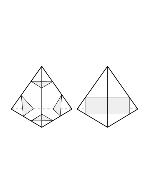
Figure 1: Elementary disks in a normal surface.

The necessary conditions given above for a vector ${\bf v}\in\mathbb{Z}^{7t}$ to be admissible are also sufficient.

Theorem 5.1

(Haken’s Hauptsatz) Let M be a triangulated compact 3-manifold with boundary, which consists of t tetrahedra. Any integer vector ${\bf v}\in\mathbb{Z}^{7t}$ that satisfies the nonnegativity conditions, matching conditions and the quadrilateral conditions gives the normal coordinates ${\bf v}(S)$ of some normal surface $S$ in $M$, which is unique up to ambient isotopy.

Proof.

This is Hauptsatz 2 of Haken [10]. It follows easily by noting that the matching conditions ensure that there is a unique way to match up the boundaries of the elementary disks specified in each tetrahedron to form a normal surface. $~{}~{}~{}\square$

This result characterizes the set ${\mathcal{W}}_{M}$ of all admissible vectors of normal surfaces as a certain set of integer points in a rational polyhedral cone in $\mathbb{R}^{7t}$. We define the Haken normal cone ${\mathcal{C}}_{M}$ to be the polyhedral cone in $\mathbb{R}^{7t}$ cut out by the nonnegativity conditions and matching conditions. The points in ${\mathcal{W}}_{M}$ are then just the integer points in the Haken normal cone ${\mathcal{C}}_{M}$ that satisfy the quadrilateral conditions.

Haken observed that the size of the integer vector ${\bf v}(S)$ measures the complexity of the normal surface. Define the weight $wt(S)$ of the normal surface $S$ to be the number of times it intersects the 1-skeleton of $M$.

Lemma 5.2

Suppose that $v_{1},v_{2},v_{3}\in\mathbb{Z}^{7t}$ lie in Haken’s normal cone ${\mathcal{C}}_{M}$ and that

$${\bf v}_{1}+{\bf v}_{2}={\bf v}_{3}~{}.$$ (3)

If ${\bf v}_{3}={\bf v}(S_{3})$ is admissible, then so are ${\bf v}_{1}$ and ${\bf v}_{2}$, so that ${\bf v}_{1}={\bf v}(S_{1})$ and ${\bf v}_{2}={\bf v}(S_{2})$. The Euler characteristics of these surfaces satisfy

$$\chi(S)=\chi(S_{1})+\chi(S_{2})~{},$$ (4)

and their weights satisfy

$$wt(S)=wt(S_{1})+wt(S_{2})~{}.$$ (5)

Proof.

The first fact follows from Theorem 5.1. For next two, Haken [10] showed that $S$ is constructed from $S_{1}$ and $S_{2}$ by a “cutting and pasting” operation called regular exchange, which yields (4) and (5). $~{}~{}~{}\square$

The “simplest” normal surfaces are thus those surfaces $S$ such that ${\bf v}(S)\neq{\bf v}(S_{1})+{\bf v}(S_{2})$ for any other (nonempty) normal surfaces $S_{1}$ and $S_{2}$. Haken calls these fundamental surfaces, and the corresponding vectors ${\bf v}(S)$ fundamental solutions. He proves that there are only finitely many fundamental surfaces; see Section 6.

Lemma 5.3

If $S$ is a fundamental surface for $(M,{\partial M})$, then $S$ is connected.

Proof.

If a normal surface $S$ is disconnected, then $S=S_{1}\cup S_{2}$ where $S_{1}$ and $S_{2}$ are disjoint nonempty normal surfaces. Now ${\bf v}(S)={\bf v}(S_{1})+{\bf v}(S_{2})$, contradicting $S$ being a fundamental surface. $~{}~{}~{}\square$

The basis of Haken’s unknotting algorithm and knot genus algorithm is the following result.

Theorem 5.4 (Haken)

Let $(M,{\partial M})$ be a triangulated compact piecewise-linear 3-manifold $M$ with nonempty boundary, which contains no embedded projective plane. If $M$ contains an essential surface with non-empty boundary, then it contains such an essential surface of minimal genus, and this surface is a fundamental normal surface.

Proof.

See Chapter 5 of Haken [10] or Section 5 of Schubert [34] or [19],[18],[20].    $\square$

This yields:

Corollary 5.5

Let $M_{K}$ be a knot complement manifold. There exists a properly embedded orientable surface $S$ in $M_{K}$ whose boundary is a longitude in $\partial M_{K}$ which is of minimal genus among all such surfaces, and which is a fundamental normal surface.

Proof.

A knot complement manifold $M_{K}$ contains no embedded projective plane, since $M_{K}$ can be embedded in ${\bf S}^{3}$. Furthermore a minimal genus surface with boundary a longitude in $\partial M_{K}$ is an essential surface in $M_{K}$ [15]. Theorem 5.4 now gives an essential surface of minimal genus which is a fundamental normal surface.   $\square$

In the special case where $K$ is unknotted, i.e. $K$ is of genus zero, Jaco and Tollefson [20] improved Haken’s criterion given in Theorem 5.4. We call a normal surface $S$ in $M$ a vertex surface if ${\bf v}(S)$ lies on an extremal ray (1-dimensional face) of the Haken normal cone ${\mathcal{C}}_{M}$. In this case we call ${\bf v}(S)$ a vertex solution of ${\mathcal{C}}_{M}$. The notion of a vertex surface was introduced by Jaco and Oertel [18], who imposed the addtional requirement that it be a connected orientable surface that is either a fundamental surface or twice a fundamental surface. The last case can occur when a surface $S$ is the boundary of a regular neighborhood of another surface which is one-sided. However $\chi(S)$ is even in this case, so that this case cannot occure when the surface is a disk.

Theorem 5.6 (Vertex Surface Theorem)

If a triangulated compact 3-manifold $M$ with nonempty boundary $\partial M$ contains an essential disk, then it contains such a disk which is a vertex surface.

Proof.

This is an immediate consequence of Corollary 6.4 of Jaco and Tollefson [20]. $~{}~{}~{}\square$

The theory of normal surfaces can also be applied to determine the splittability of links.

Theorem 5.7 (Splittability Criterion)

A link $L$ is splittable if and only if any link complement manifold $M_{L}$ contains a fundamental normal 2-sphere $S$ that separates two components of $\partial M_{L}$.

Proof.

This is established in Section 4 of Schubert [34], who attributes the result to Haken [10]. See also [19] [20]   $\square$

This result was strengthened by Jaco and Tollefson [20].

Theorem 5.8

If a link complement manifold $M_{L}$ contains a normal 2-sphere $S$ which separates two components of $\partial M_{L}$, then it contains such a sphere that is a vertex surface.

Proof.

This follows from Theorem 5.2 [20].   $\square$

To check that a sphere $S$ separates two components of $\partial M_{L}$ it suffices to exhibit a path in the 1-skeleton of $M_{L}$ that connects two components of $\partial M_{L}$ and whose intersection number with $S$ is odd.

For the complexity analysis, we must give bounds for the number of vectors ${\bf v}$ in the exhausting set, and for the sizes $||{\bf v}||_{1}$ of these vectors, where the size is

$$||{\bf v}||_{1}:=\sum_{i=1}^{7t}v_{i}~{}.$$ (6)

We address these questions in the next section. Then in Section 7 we deal with the problem of constructing the triangulated 3-manifold $M_{K}={\bf S}^{3}-R_{K}$ from a knot diagram ${\mathcal{K}}$. Sections 8–10 give the complexity analysis.

6 Bounds for Fundamental Solutions and Hilbert Bases

We bound the number and size of fundamental solutions in the Haken normal cone ${\mathcal{C}}_{M}$ of an arbitrary triangulated compact 3-manifold $M$ with boundary $\partial M$ that contains $t$ tetrahedra. The system of linear inequalities defining Haken’s normal cone ${\mathcal{C}}_{M}$ has the form:

$$v_{i}\geq 0\quad(1\leq i\leq 7t)~{},$$ (7)

$$v_{k_{1}}+v_{k_{2}}=v_{k_{3}}+v_{k_{4}}\quad\mbox{(at most}~{}6t~{}\mbox{equations})~{}.$$ (8)

The matching conditions (8) all involve exactly four variables as indicated, because only two of the seven disk types in a tetrahedron $T$ have edges parallel to one specified edge on one face of $T$. There are at most $6t$ such equations because the $t$ tetrahedra have between them $12t$ such edge pairs, and each equation matches two pairs that occur in no other equation. (There will be strictly less than $6t$ equations if $M$ has nonempty boundary.) The cone ${\mathcal{C}}_{M}$ is a pointed cone, (i.e. it contains no line) because it is contained in the positive orthant $\mathbb{R}^{7t}_{+}$. It is not full-dimensional because it has equality constraints, but (8) implies

$$t\leq\dim_{\mathbb{R}}({\mathcal{C}}_{M})\leq 7t~{}.$$ (9)

It is a rational cone because it is cut out by rational equality and inequality constraints; equivalently, each of its extreme rays contains an integral vector. The concept of fundamental solutions of ${\mathcal{C}}_{M}$ is closely related to that of a Hilbert basis for the rational cone ${\mathcal{C}}_{M}$. Given a (homogeneous) rational cone ${\mathcal{C}}$ in $\mathbb{R}^{m}$, its set of integral points

$${\mathcal{C}}(\mathbb{Z}):={\mathcal{C}}\cap\mathbb{Z}^{m}$$ (10)

forms a semigroup under addition. An (integral) Hilbert generating set ${\mathcal{G}}$ for ${\mathcal{C}}$ is any finite set of generators for ${\mathcal{C}}(\mathbb{Z})$. If ${\mathcal{C}}$ is a pointed rational cone, then ${\mathcal{C}}$ has a unique minimal generating set ${\mathcal{H}}$, see Schrijver[33, Theorem 16.4]. It consists exactly of all elements ${\bf v}\in{\mathcal{C}}(\mathbb{Z})$ which are minimal in the sense that

$${\bf v}\neq{\bf v}_{1}+{\bf v}_{2}\quad\mbox{for any nonzero}~{}~{}{\bf v}_{1},{\bf v}_{2}\in{\mathcal{C}}(\mathbb{Z})~{}.$$ (11)

We call this set ${\mathcal{H}}={\mathcal{H}}({\mathcal{C}})$ the minimal Hilbert basis of ${\mathcal{C}}$. By definition, any fundamental solution of ${\mathcal{C}}_{M}$ is in the minimal Hilbert basis ${\mathcal{H}}({\mathcal{C}}_{M})$. There may, however, be elements in ${\mathcal{H}}({\mathcal{C}}_{M})$ that are not fundamental solutions because they violate the quadrilateral conditions.

A minimal vertex solution of a pointed homogeneous rational cone ${\mathcal{C}}$ in $\mathbb{R}^{m}$ is the smallest nonzero integral point on any extreme ray (1-dimensional face) of the cone ${\mathcal{C}}$. A minimal vertex solution is always in the minimal Hilbert basis ${\mathcal{H}}({\mathcal{C}})$, because the only points in ${\mathcal{C}}$ that it can be a convex combination of are other points in the ray $\mathbb{R}^{+}{\bf v}=\{\lambda{\bf v}:\lambda\geq 0\}$. By definition a fundamental vertex solution of the Haken cone ${\mathcal{C}}_{M}$ is a minimal vertex solution of ${\mathcal{C}}_{M}$.

Lemma 6.1

Let $M$ be a triangulated compact 3-manifold, possibly with boundary, that contains $t$ tetrahedra in the triangulation.

• Any vertex minimal solution ${\bf v}\in\mathbb{Z}^{7t}$ of the Haken normal cone ${\mathcal{C}}_{M}$ in $\mathbb{R}^{7t}$ has

  $$\max_{1\leq i\leq 7t}(v_{i})\leq 2^{7t-1}~{}.$$ (12)

• Any minimal Hilbert basis element ${\bf v}\in\mathbb{Z}^{7t}$ of the Haken normal cone ${\mathcal{C}}_{M}$ has

  $$\max_{1\leq i\leq 7t}(v_{i})\leq t\cdot 2^{7t+2}~{}.$$ (13)

Proof.

• Choose a maximal linearly independent subset of matching conditions (8). There will be $7t-d$ of them, where $d=\dim_{\mathbb{R}}({\mathcal{C}}_{M})$. Any vertex ray is determined by adjoining to these equations $d-1$ other binding inequality constraints

  $$\{{\bf v}_{i_{k}}=0~{};\quad 1\leq k\leq d-1\}~{},$$ (14)

  with the proviso that the resulting system have rank $7t-1$. These conditions yield a $(7t-1)\times 7t$ integer matrix ${\bf{M}}$ of rank $7t-1$, and the vertex ray elements ${\bf z}=(z_{1}{,\ldots,}z_{7t})$ satisfy

  $${\bf{M}}{\bf z}={\bf 0}~{}.$$ (15)

  In order to get a feasible vertex ray in ${\mathcal{C}}_{M}$ all nonzero coordinates $z_{i}$ must have the same sign.

  At least one of the unit coordinate vectors ${\bf e}_{1},{\bf e}_{2}{,\ldots,}{\bf e}_{7t}$ must be linearly independent of the row space of ${\bf{M}}$. Adjoin it as a first row to ${\bf{M}}$ and we obtain a full rank $7t\times 7t$ integer matrix

  $$\tilde{{\bf{M}}}=[\begin{array}[]{c}{\bf e}_{k}\\ {\bf{M}}\end{array}]~{},\quad\det(\tilde{{\bf{M}}})\neq 0~{}.$$

  Consider the adjoint matrix $adj(\tilde{{\bf{M}}})=\det(\tilde{{\bf{M}}})\tilde{{\bf{M}}}^{-1}$, which has integer entries

  $$w_{ij}:=adj(\tilde{{\bf{M}}})_{ij}=(-1)^{i+j}\det\tilde{{\bf{M}}}[j|i]~{},$$ (16)

  in which $\tilde{{\bf{M}}}[j|i]$ is the minor obtained by crossing out the $j^{\rm th}$ row and $i^{\rm th}$ column of $\tilde{{\bf{M}}}$. Let

  $${\bf w}=[w_{11},w_{21}{,\ldots,}w_{7t,1}]^{t}$$ (17)

  be the first column of $adj(\tilde{{\bf{M}}})$. Since $\tilde{{\bf{M}}}adj(\tilde{{\bf{M}}})=\det(\tilde{{\bf{M}}}){\bf{M}}$ this yields

  $$\tilde{{\bf{M}}}{\bf w}={\bf 0}~{},$$

  and ${\bf w}\neq{\bf 0}$ because $\langle{\bf e}_{k},{\bf w}\rangle=\det(\tilde{{\bf{M}}})\neq 0$. We bound the entries of ${\bf w}$ using Hadamard’s inequality, which states for an $m\times m$ real matrix that

  $$\det({\bf{N}})^{2}\leq\prod_{i=1}^{m}||{\bf n}_{i}||^{2}~{},$$

  in which $||{\bf n}_{i}||^{2}$ is the Euclidean length of the $i^{\rm th}$ row ${\bf n}_{i}$ of ${\bf{N}}$. We apply this to (15), and observe that each row of the $(7t-1)\times(7t-1)$ matrix $\tilde{{\bf{M}}}[j|i]$ has squared Euclidean length at most 4, because this is true for all row vectors in the system given by (8) and for ${\bf e}_{k}$. Applied to (15) this gives

  $$|w_{ij}|^{2}\leq 4^{7t-1}~{}.$$

  However (15) shows that ${\bf w}\in\mathbb{Z}^{7t}$, and a vertex minimal solution ${\bf v}$ in the extreme ray is obtained by dividing ${\bf w}$ by the greatest common divisor of its elements, hence

  $$\max_{1\leq i\leq 7t}|v_{i}|\leq\max_{1\leq i\leq 7t}|w_{i1}|\leq 2^{7t-1}~{}.$$

• A simplicial cone ${\mathcal{C}}$ in $\mathbb{R}^{7t}$ is a $d$-dimensional pointed cone which has exactly $d$ extreme rays. Let ${\bf v}^{(1)}{,\ldots,}{\bf v}^{(d)}\in\mathbb{Z}^{7t}$ be the vertex minimal solutions for the extreme rays. Each point in ${\mathcal{C}}$ can be expressed as a nonnegative linear combination of the ${\bf v}^{(j)}$, as

  $${\bf v}=\sum_{j=1}^{d}\lambda_{j}{\bf v}^{(j)}~{},\quad\mbox{each}~{}~{}\lambda_{j}\geq 0~{}.$$

  If ${\bf v}$ is in the minimal Hilbert basis ${\mathcal{H}}({\mathcal{C}})$, then $0\leq\lambda_{j}\leq 1$, for otherwise one has

  $${\bf v}=({\bf v}-{\bf v}^{(j)})+{\bf v}^{(j)},$$

  and both ${\bf v}-{\bf v}^{(j)}$ and ${\bf v}^{(j)}$ are nonzero integer vectors in ${\mathcal{C}}$, which is a contradiction. Thus, any minimal Hilbert basis element ${\bf v}=(v_{1},\ldots,v_{7t})$ of a simplicial cone satisfies

  $$|v_{i}|\leq\sum_{j=1}^{d}|v_{i}^{(j)}|\quad\mbox{for}~{}~{}1\leq i\leq 7t~{}.$$ (18)

  The cone ${\mathcal{C}}_{M}$ may not be simplicial, but we can partition it into a set of simplicial cones $\{{\mathcal{C}}_{M}^{(k)}\}$ each of whose extreme rays are extreme rays of ${\mathcal{C}}_{M}$ itself. We have

  $${\mathcal{H}}({\mathcal{C}}_{M})\subseteq\bigcup_{k}{\mathcal{H}}({\mathcal{C}}_{M}^{(k)})~{}.$$

  Thus all Hilbert basis elements of ${\mathcal{H}}({\mathcal{C}}_{M})$ satisfy by the bound in (18) for Hilbert basis elements of ${\mathcal{H}}({\mathcal{C}}_{M}^{(k)})$. Using (12) to bound $|v_{i}^{(j)}|$ we obtain

  $$|v_{i}|\leq d2^{7t-1}\leq 7t~{}2^{7t-1}\leq t~{}2^{7t+2}~{},$$

  as required. $~{}~{}~{}\square$

Lemma 6.2

• The Haken normal cone ${\mathcal{C}}_{M}$ has at most $2^{7t}$ vertex fundamental solutions.

• The Haken normal cone ${\mathcal{C}}_{M}$ has at most $t^{7t}~{}2^{49t^{2}+14t}$ elements in its minimal Hilbert basis.

Proof.

• There are ${7t}\choose{d-1}$ possible choices for the systems given in (14), and ${{7t}\choose{d-1}}\leq 2^{7t}$.

• We wastefully count every integer vector ${\bf v}$ in the box $0\leq v_{i}\leq t2^{7t+2}$ for $1\leq i\leq 7t$ that is allowed by Lemma 6.1. $~{}~{}~{}\square$

Remark.

The bounds in Lemma 6.2 are very crude. However the functional forms $2^{c_{1}t}$ and $2^{c_{2}t^{2}}$ of the bounds are best possible for general rational cones, apart from the values of $c_{1}$ and $c_{2}$.

7 Triangulations

Given a link diagram ${\mathcal{D}}$ with crossing measure $n$, we show how to construct a triangulated 3-manifold $M_{L}\cong{\bf S}^{3}-R_{L}$, where $R_{L}$ is a regular neighborhood of a link $L$ which has a regular projection that is the link diagram ${\mathcal{D}}$. The construction takes time polynomial in the crossing measure of ${\mathcal{D}}$, and the triangulations of each of $M_{L}$ and $\bar{R}_{L}$ contain $O(n)$ tetrahedra.

Lemma 7.1

Given a link diagram ${\mathcal{D}}$ of crossing measure $n$, one can construct in time $O(n\log n)$ a triangulated convex polyhedron P in $\mathbb{R}^{3}$ such that:

1. The triangulation has at most $420n$ tetrahedra.

2. Every vertex in the triangulation is a lattice point $(x,y,z)\in\mathbb{Z}^{3}$, with $0\leq x\leq 30n$, $0\leq y\leq 30n$ and $-4\leq z\leq 4$.

3. There is a link L embedded in the 1-skeleton of the triangulation which lies entirely in the interior of $P$, and whose orthogonal projection on the $(x,y)$-plane is regular and is a link diagram isomorphic to ${\mathcal{D}}$.

Proof.

We first add extra vertices to ${\mathcal{D}}$. To each non-loop edge we add a new vertex of degree 2, which splits it into two edges. To each non-isolated loop we add two new vertices of degree 2, which split it into three edges. To each isolated loops we add three new vertices of degree 2, making it an isolated triangle. The resulting labelled graph ${\mathcal{G}}$ is still planar, has no loops or multiple edges, and has at most $5n$ vertices. (The worst case consists of several disjoint single crossing projections.) Let $m$ denote the number of vertices of ${\mathcal{G}}$, and call the $m-n$ vertices added special vertices.

Using the Hopcroft-Tarjan planarity testing algorithm [17] we can construct a planar embedding of ${\mathcal{G}}$ in time $O(n\log n)$. From this data we determine the planar faces of this embedding, and add extra edges to triangulate each face, thus obtaining a triangulated planar graph ${\mathcal{G}}^{\prime}$, in time $O(n)$. The graph ${\mathcal{G}}^{\prime}$ has $m$ vertices and $2m-5$ bounded triangular faces, and the unbounded face is also a triangle.

It was shown by de Frajsseix, Pach and Pollack [7] that there exists a planar embedding of ${\mathcal{G}}^{\prime}$ whose vertices $v({\mathcal{G}}^{\prime})$ lie in the plane $z=-1$, in the grid

$$\{(x,y,-1):0\leq x,y\leq 10n-1~{};\quad x,y\in\mathbb{Z}\}~{},$$ (19)

in which all edges of ${\mathcal{G}}^{\prime}$ are straight line segments. They also show in [7, Section 4] that one can explicitly find such an embedding in time $O(n\log n)$.

Next we make an identical copy ${\mathcal{G}}^{\prime\prime}$ of ${\mathcal{G}}^{\prime}$ on the plane $z=1$ with ${\mathcal{G}}^{\prime\prime}={\mathcal{G}}+(0,0,2)$, and vertex set $V({\mathcal{G}}^{\prime\prime})=V({\mathcal{G}})+(0,0,2)$. We now consider the polyhedron $P^{\prime}$ which is the convex hull of $V({\mathcal{G}}^{\prime})$ and $V({\mathcal{G}}^{\prime\prime})$. It is a triangular prism, because the outside face of ${\mathcal{G}}^{\prime}$ is a triangle. We add $m_{1}$ vertical edges connecting each vertex ${\bf v}\in V({\mathcal{G}}^{\prime})$ to its copy ${\bf v}+(0,0,1)\in V({\mathcal{G}}^{\prime\prime})$. Let ${\mathcal{E}}$ denote these edges, together with all the edges in ${\mathcal{G}}^{\prime}$ and ${\mathcal{G}}^{\prime\prime}$. Using these edges, the polyhedron $P^{\prime}$ decomposes into $2m-5$ triangular prisms $\{Q_{j}:1\leq j\leq 2m-5\}$, with top and bottom faces of each being congruent triangular faces of ${\mathcal{G}}^{\prime}$ and ${\mathcal{G}}^{\prime\prime}$.

We next triangulate $P^{\prime}$ by dissecting each of the $2m-5$ triangular prisms into 14 tetrahedra, as follows. We subdivide each vertical rectangular face into four triangles using its diagonals. Then we cone each rectangular face to the centroid of $P^{\prime}$, and note that the centroid lies in the plane $z=0$. We add 4 new vertices to each prism, one on each face and one in the center. The point of this subdivision is that the triangulations of adjacent prisms are compatible. Note also that all new vertices added lie in the lattice $\displaystyle\frac{1}{6}\mathbb{Z}^{2}$.

Let ${\mathcal{E}}^{\prime}$ denote all the edges in the union of these triangulated prisms. We identify the link diagram ${\mathcal{D}}$ with the graph ${\mathcal{G}}$ embedded in ${\mathcal{G}}^{\prime}$. We next observe that there is a polygonal link $L$ imbedded in the edge set ${\mathcal{E}}^{\prime}$ whose projection is the link diagram ${\mathcal{D}}$. We insist that any edge in ${\mathcal{D}}$ that runs to an undercrossing have its undercrossing vertex lie in the plane $z=-1$, while any edge that runs to an overcrossing has its overcrossing vertex lie in the plane $z=1$. Each such edge travels from one of the $n$ original vertices of ${\mathcal{D}}$ to a special vertex. Edges that do not meet vertices labelled overcrossing or undercrossing are assigned to the $z=-1$ plane. The edge corresponding to an edge running from the $z=-1$ to the $z=1$ plane is contained in one of the diagonals added to a prism. The resulting embedding $L$ in $P^{\prime}$ has a regular orthogonal projection onto the $(x,y)$-plane, since no edges are vertical and only transverse double points occur as singularities in the projection.

The knot edges lie in the boundary of $P^{\prime}$. To correct this we take two additional copies of $P^{\prime}$ and glue one to its top, along the plane $z=1$, and one to its bottom, along the plane $z=-1$. The knot now lies in the interior of the resulting polyhedron $P^{\prime\prime}$. All the vertices added in this construction lie in $\displaystyle\frac{1}{6}\mathbb{Z}^{3}$, so a rescaling by a factor of 6 puts all vertices in $\mathbb{Z}^{3}$. The total number of tetrahedra used in triangulating $P^{\prime\prime}$ is $84m$, which is at most $420n$.

Now $P^{\prime\prime}$ satisfies properties (i), (ii) and (iii).$~{}~{}~{}\square$

We now construct a triangulated 3-manifold $M_{L}$ embedded in ${\bf S}^{3}$ from the triangulation of $P$ in Lemma 5.2. This construction only uses the combinatorial triangulation of $P$, i.e. the adjacency relations of tetrahedra and of the set of edges of $P$ that specify the link $L$, and does not use its given embedding in $\mathbb{R}^{3}$.

Lemma 7.2

Given a link diagram ${\mathcal{D}}$ of crossing measure n, one can construct in time $O(n\log n)$ a combinatorial triangulation of ${\bf S}^{3}$ using at most $253440(n+1)$ tetrahedra, which contains a good triangulation of $M_{L}\cong{\bf S}^{3}-R_{L}$, with $\bar{R}_{L}$ a regular neighborhood of a combinatorial link $L$ with link diagram ${\mathcal{D}}$, and $\partial R_{L}=\partial M_{K}$. Furthermore one can construct in time $O(n^{2}\log n)$ in the triangulation marked sets of edges in $\partial M_{L}$ for a meridian on each 2-torus component of $\partial M_{L}$, and a set of marked paths of $O(n)$ edges in $M_{L}\setminus\partial M_{L}$ that connect pairs of components of $\partial M_{L}$, which between them connect all components of $\partial M_{L}$.

Proof.

We construct a combinatorial triangulation ${\mathcal{T}}$ of ${\bf S}^{3}$ by coning all the triangular outside faces of the triangulation of $P$ to the “point at infinity” added in constructing ${\bf S}^{3}$ as the one point compactification of $\mathbb{R}^{3}$. This adds $4m+2$ new tetrahedra, where $m\leq 5n$, for a total of at most $440n+2$ tetrahedra. Barycentrically subdivide twice to obtain a triangulation ${\mathcal{T}}^{\prime\prime}$, and take $M_{L}$ to be ${\bf S}^{3}$ minus the interior of a regular neighborhood of $L$. Since barycentric subdivision splits a tetrahedron into 24 tetrahedra, we use at most $24^{2}(440n+2)$ tetrahedra. It is easy to determine a meridian on the 2-torus in $\partial M_{L}$ corresponding to each component of $L$, in time $O(n)$. To construct a longitude we use the projection of the polyhedron $P$ in $\mathbb{R}^{3}$ on the z-axis in Lemma 7.1 to construct a path with algebraic linking number zero with the core of the 2-torus. This can be done by suitably making a “twist” at each vertex.

We can find a shortest path between each pair of components of $\partial M_{K}$ in time $O(n\log n)$ each. We retain a minimal set of such paths which contain no edge inside any component of $\partial M_{K}$, whose union connects all components of $\partial M_{K}$. If done carefully, this can be done in time $O(n^{2}\log n)$ and result in a list of at most $O(n)$ paths involving $O(n^{2})$ edges.   $\square$

8 Certifying Unknottedness

To show that the unknottedness problem is in NP, we must construct for any $n$-crossing knot diagram ${\mathcal{D}}$ a polynomial length certificate that proves it is unknotted. The certificate takes the following form.

Unknottedness Certificate

1. Given a link diagram ${\mathcal{D}}$ with $n$ crossings certify that ${\mathcal{D}}$ is a knot diagram.

2. Construct a piecewise-linear knot $K$ in $\mathbb{R}^{3}$ which has regular projection ${\mathcal{D}}$. From it construct a good triangulation $M_{K}\cong{\bf S}^{3}-\bar{R}_{K}$ which contains $t$ tetrahedra, with $t=O(n)$, and with a meridian of $\partial R_{K}$ marked in $\partial M_{K}$.

3. Guess a suitable fundamental solution ${\bf v}\in\mathbb{Z}^{7t}$ to the Haken normal equations for $M_{K}$. Verify the Haken quadrilateral conditions. Let $S$ denote the associated normal surface, so ${\bf v}={\bf v}(S)$.

4. Certify that $S$ is an essential disk.

   (4a) Certify that $S$ is connected.

   (4b) Certify that $S$ is a disk. Check that $\partial S\neq\emptyset$ and that it has Euler characteristic $\chi(S)=1$.

   (4c) Certify that $S$ is essential by checking that its homology class $[\partial S]\neq(0,0)$ in $H_{1}(\partial M_{K};\mathbb{Z}/2\mathbb{Z})$.

The approach of Haken to deciding unknottedness is based on an exhaustive search for a certificate of the above kind.

Haken-type Unknottedness Algorithm

Input: Link diagram ${\mathcal{D}}$ of crossing number $n$.

Question: Is ${\mathcal{D}}$ a knot diagram of the unknot?

1. Test if ${\mathcal{D}}$ is a knot diagram. If so, denote it ${\mathcal{K}}$.

2. Construct a finite combinatorial triangulation ${\mathcal{T}}$ of ${\bf S}^{3}$ which contains a polygonal knot $K$ in its one-skeleton which has diagram ${\mathcal{K}}$, and also contains a good compact triangulated 3-manifold $M_{K}\cong{\bf S}^{3}-R_{K}$, where $\bar{R}_{K}$ is a regular neighborhood of $K$. Let $t$ denote the number of tetrahedra in $M_{K}$.

3. Construct an exhausting list ${\mathcal{L}}$ of vectors ${\mathcal{L}}\subseteq\mathbb{Z}^{7t}$ that contains ${\bf v}(S)$ for some embedded compressing disk in $M_{K}$, if one exists.

4. For each ${\bf v}\in{\mathcal{L}}$, test if ${\bf v}$ is admissible. If so let $S$ denote the normal surface with ${\bf v}={\bf v}(S)$. Test if $S$ is an essential disk for $M_{K}$.

   (4a) Is $S$ connected?

   (4b) Is $S$ a disk? Check that the Euler characteristic $\chi(S)=1$ and $\partial S\neq\emptyset$.

   (4c) Is $S$ essential? Check that the homology class $[\partial S]\in H_{1}(\partial M;\mathbb{Z}/2\mathbb{Z})$ is nontrivial by computing that its intersection number $(\bmod~{}2)$ with a meridian of the 2-torus $T_{K}$ is $1\ (\bmod~{}2)$.

   If all tests are passed for $S$, answer “yes,” halt and output ${\bf v}(S)$.

5. If the complete list ${\mathcal{L}}$ is examined and no essential disk is found, answer, “no” and halt.

For the Haken unknottedness algorithm we take for the Exhausting List ${\mathcal{L}}_{H}:={\mathcal{L}}_{H}(M_{K})$ the set

$${\mathcal{L}}_{H}:=\{{\bf v}=(v_{1}{,\ldots,}v_{7t})\in\mathbb{Z}^{7t}:0\leq v_{i}\leq t2^{7t+2}\}~{}.$$ (20)

For the Jaco-Tollefson unknottedness algorithm we take for the exhausting list ${\mathcal{L}}_{V}={\mathcal{L}}_{{\bf v}}(M_{K})$ the set

$${\mathcal{L}}_{V}:=\{{\bf v}=(v_{1}{,\ldots,}v_{7t})\in\mathbb{Z}^{7t}:{\bf v}~{}~{}\mbox{a minimal vertex solution in}~{}~{}{\mathcal{C}}_{M}\}~{}.$$ (21)

Theorem 8.1

• There is a constant $c$ such that the Haken unknottedness algorithm decides for any $n$-crossing link diagram whether it is a knot diagram that represents the trivial knot using at most $O(\exp(cn^{2}))$ time and $O(n^{2}\log n)$ space, on a Turing machine.

• There is a constant $c^{\prime}$ such that the Jaco-Tollefson unknottedness algorithm decides the same question in at most time $O(\exp(c^{\prime}n))$ time and $O(n^{2}\log n)$ space, on a Turing machine.

Proof.

Assuming that the individual steps of the algorithms are proved correct, the two algorithms are correct by Lemmas 4.1 and 4.2, respectively.

(1) For the Haken unknottedness algorithm, the list ${\mathcal{L}}_{H}$ is exhausting by Theorem 5.4 with Lemma 4.1.

Step (1) is done in polynomial time $O(n\log n)$ by tracing a path through the link diagram ${\mathcal{D}}$ and checking that it visits every edge of ${\mathcal{D}}$.

Step (2) is done in polynomial time $O(n\log n)$ by Lemmas 7.1 and 7.2. The triangulated manifold $M_{K}$ has at most $253440(n+1)$ tetrahedra.

The list ${\mathcal{L}}_{H}$ is a large cube containing $t^{7t}2^{49t^{2}+14t}$ integer vectors, using integers containing at most $7t+\log_{2}t+2$ binary digits. We now test each ${\bf v}\in{\mathcal{L}}_{H}$, one at a time, to determine whether it is a fundamental solution that is an essential disk.

To begin step (4), given ${\bf v}\in{\mathcal{L}}_{H}$, we first test whether ${\bf v}$ corresponds to a normal surface by checking whether the quadrilateral conditions hold: for each tetrahedron in $M_{K}$ at least two of the three quadrilateral variables vanish. This takes time $O(t)$ and space $O(t^{2})$. Now we have ${\bf v}={\bf v}(S)$ for some normal surface $S$. We can treat $S$ as a triangulated surface by splitting quadrilaterals into four triangles by adding two diagonals to each quadrilateral.

If $S$ is connected, then we can check whether $S$ is homeomorphic to a disk in polynomial time $O(n^{2}\log n)$. We use the criterion of Lemma 4.3. We check that $\partial S\neq\emptyset$ by checking that $v_{i}\neq 0$ for some triangle or quadrilateral is that has an edge in $\partial M$. We can compute the Euler characteristic $\chi(S)$ in polynomial time directly from the data in ${\bf v}$, since it encodes the necessary data on the vertices, edges and faces of the triangles and quadrilaterals in $S$. According to Jaco and Tollefson [20, p. 404] we have

$$\chi(S)=\displaystyle\frac{1}{2}S_{3}-\sigma(S)+wt(S)$$ (22)

in which $S_{3}$ counts the total number of triangles in $S$, $\sigma(S)=\sum_{i=1}^{7t}v_{i}$, and wt(S) is defined below. For each edge $j$ in the triangulation of $M_{K}$, let $t_{j}$ count the number of tetrahedra that contain edge $j$, and set $\epsilon_{ji}=1$ if edge $e_{j}$ meets a disk of type $i$. Then

$$wt(S)=\sum_{i=1}^{7t}\sum_{j}\displaystyle\frac{\epsilon_{ji}v_{i}}{t_{j}}~{}.$$ (23)

The weight counts the intersection of $S$ with the 1-skeleton of the triangulation. Thus $\chi(S)$ is computed by (22) using $O(n^{2}\log n)$ bit operations, and we can check whether $\chi(S)=1$.

If $S$ is known to be a disk, then we can check whether $\partial S$ is an essential curve in $\partial M$ in polynomial time. Since $S$ is a disk the boundary $\partial S$ must have homology class $(0,0)$ or $(0,\pm 1)$ in $H_{1}(\partial M;\mathbb{Z})$, by Lemma 4.1. We distinguish these possibilities by determining if the class $[\partial S]\in H_{1}(\partial M_{1};\mathbb{Z}/2\mathbb{Z})$ is $(0,0)$ or $(0,1)$. To do this we compute the intersection number $(\bmod~{}2)$ of $\partial S$ with a fixed meridian in the 1-skeleton of the 2-torus $\partial M_{K}$. Such a meridian $\gamma$ can be determined in time $O(n\log n)$ in the process of constructing $M_{K}$ in step (2). This intersection number can be computed in time $O(n\log n)$ as

$$n_{S}:=\displaystyle\frac{1}{2}(\sum v_{i})~{}~{}(\bmod~{}2)~{},$$ (24)

in which the sum is taken over those disk types $i$ that correspond to triangles and quadrilaterals with an edge on $\partial M_{K}$ and a vertex on that edge that is contained in some edge of $\gamma$. We count disk types $i$ with multiplicity equal to the number of vertices of this type contained in the disk type. Then $S$ is essential only if $n_{s}\equiv 1(\bmod~{}2)$, using Lemma 4.2.

Thus to test a given ${\bf v}\in{\mathcal{L}}_{H}$ requires $O(t^{7t}2^{49t^{2}+14t})$ operations, and testing $S$ for being a fundamental solution is the only step that requires exponential time.

The total running time of the Haken algorithm is dominated by the test for being a fundamental solution and the size of the exhausting list ${\mathcal{L}}_{H}$. It is easy to sequentially test elements of ${\mathcal{L}}_{H}$ in lexicographic order, so that the space complexity does not materially increase over that for testing a single vector ${\bf v}$. Since $t\leq O(n)$ we obtain upper bounds of the form $O(2^{cn^{2}})$ for time complexity and $O(n^{2}\log n)$ for the space complexity.

(2). For the Jaco-Tollefson algorithm, the list ${\mathcal{L}}_{V}$ is exhausting by the Vertex Surface Theorem 5.6 and Lemma 6.1. There are at most $2^{7t}$ elements in ${\mathcal{L}}_{V}$ by Lemma 6.2. Furthermore these elements are easy to enumerate sequentially in time $O(\log n)$ each: First precompute a maximal linearly independent set of $7t-d$ matching condition constraints, where $d=\dim_{\mathbb{R}}({\mathcal{C}}_{M})$. Then test all $(d-1)$-duples $\{i_{1}{,\ldots,}i_{d-1}\}\subseteq\{1,2{,\ldots,}7t\}$ to see if adjoining the constraints

$$x_{i_{j}}=0~{},\quad 1\leq j\leq d$$

gives an extremal ray of the Haken cone ${\mathcal{C}}_{M}$. If so, determine a minimal point ${\bf v}\in\mathbb{Z}^{7t}$ on this ray and run the rest of the algorithm. Given $\{i_{1}{,\ldots,}i_{j}\}$ one can compute ${\bf v}$ in polynomial time $O(n^{2}\log n)$ by first computing ${\bf w}$ in (16) and dividing it by g.c.d. $(w_{1},w_{2}{,\ldots,}w_{7t})$ to get ${\bf v}$.

The testing time, for each ${\bf v}\in{\mathcal{L}}_{V}$, for whether ${\bf v}={\bf v}(S)$ gives an essential disk $S$ goes down to $O(t2^{7t})$ time and to $O(n^{2}\log n)$ space, because the computationally intensive test whether $S$ is connected is eliminated: $S$ is connected because minimal vertex solutions are always Hilbert basis elements, so $S$ is a fundamental surface and connected by Lemma 5.2.

Since $t=O(n)$ we obtain the time bound $O(2^{cn})$ and space bound at most $O(n^{2}\log n)$.

We check whether $S$ is fundamental by exhaustive search. For each ${\bf w}\in\mathbb{Z}^{7t}$ with $0\leq w_{i}\leq v_{i}$ for $1\leq i\leq 7t$ we set ${\bf w}^{\prime}={\bf v}-{\bf w}$ and check if ${\bf w},{\bf w}^{\prime}\in{\mathcal{C}}_{M}$. If this happens for some ${\bf w}$ then ${\bf v}={\bf w}+{\bf w}^{\prime}$ is not fundamental. If this happens for no ${\bf w}$ then ${\bf v}$ is in the Hilbert basis, and is a fundamental surface by Lemma 5.2. There are at most $O(t^{7t}2^{49t^{2}+14t})$ values of ${\bf w}$ to check. We can check them sequentially, using space $O(t^{2})$. If $S$ is a fundamental surface, then it is guaranteed to be connected by Lemma 5.3.   $\square$

We can now prove that the Unknottedness Certificate above can be checked in polynomial time.

Proof of Theorem 1.1

If all the steps in the certificate are checked then ${\mathcal{D}}$ is unknotted by Lemma 4.2. It remains to show each step can be done in length polynomial in $n$.

1. This is trivially polynomial time in $n$, by tracing edges around the graph.

2. This is polynomial time by Lemma 7.2, upon observing that $t=O(n)$.

3. This step is nondeterministic. According to Lemma 6.1, any fundamental solution is

   $$wt({\bf v})\leq\sum_{i=0}^{7t}v_{i}\leq 7t^{2}2^{7t+2}~{},$$

   hence ${\bf v}$ can be guessed in nondeterministic time linear in $t$, which is $O(n)$. At this point we do not have a proof that the solution is fundamental. Verifying the quadrilateral conditions takes time $O(n^{2})$, since we have $O(n)$ tetrahedra and have $O(n)$-bit integers in ${\bf v}$ to examine.

(4a) According to the Vertex Surface Theorem (5.6), we may choose a vertex fundamental solution in (3) for which $S$ is an essential disk. We may certify in polynomial time that ${\bf v}={\bf v}(S)$ is in the Hilbert basis, by guessing the correct linearly independent set of $7t-1$ constraints that are binding for ${\bf v}$, and then verifying that ${\bf v}\in\mathbb{Z}^{7t}$ is primitive, i.e.

$$g.c.d.(v_{1},v_{2}{,\ldots,}v_{7t})=1~{}.$$

This takes time $O(n^{3}\log n)$. We verify the $7t-1$ constraints are linearly independent by guessing which one of the unit coordinate vectors ${\bf e}_{1}{,\ldots,}{\bf e}_{7t}$ extends to a basis of $\mathbb{R}^{7t}$ and verifying that the determinant of the resulting matrix is nonzero. (We also must check that all equality constraints are satisfied.) Since ${\bf v}$ is in the Hilbert basis and the quadrilateral conditions hold, $S$ is connected by Lemma 5.3.

(4b) and (4c) were shown to take polynomial time in the proof of Theorem 8.1. $~{}~{}~{}\square$

Using Haken’s Theorem 5.4 instead of the Jaco-Tollefson result we still obtain the weaker result that the unknotting problem is in the polynomial hierarchy $\Sigma_{2}^{p}$ [38]: One uses the same certificate as above, except for the proof that $S$ is connected. For this step, we use a co-NP. oracle that answers the question: Is ${\bf v}$ in the Hilbert basis of ${\mathcal{C}}_{M}$? This problem is in co-NP, because one can certify that ${\bf v}$ is not in the Hilbert basis by guessing ${\bf v}_{1},{\bf v}_{2}\in{\mathcal{C}}_{M}$ such that ${\bf v}={\bf v}_{1}+{\bf v}_{2}$. This puts the problem in the complexity class $\mbox{\bf NP}^{\mbox{\bf co-NP}}=\mbox{\bf NP}^{\mbox{\bf NP}}=\Sigma_{2}^{p}$. A stronger result than this cannot be expected, since it is known that the problem of testing whether a vector ${\bf v}$ is in the Hilbert basis of a pointed rational cone ${\mathcal{C}}$ is co-NP complete, see Sebö [35, Theorem 5.1].

9 Certifying Splittability

We treat the splitting problem with a modification of the method described above. We use the criterion for splittability of a link given in Theorem 5.7. The construction of the certificate, and its verification, take place in the following steps.

Splitting Link Certificate.

1. Given a link diagram ${\cal D}$, construct a piecewise-linear link $L$ in $\mathbb{R}^{3}$ that has regular projection ${\cal D}$. From it construct a good triangulation of $M_{L}\cong{\bf S}^{3}-R_{L}$ which contains $t$ tetrahedra, with $t=O(n)$, and with a meridian marked in each component of $\partial M_{L}$. (Use Lemma 7.1.)

2. Guess a suitable vertex solution ${\bf v}\in\mathbb{Z}^{7t}$ to the Haken normal equations for $M_{L}$. (This solution can be written in polynomial length by Lemma 6.1.) Verify the quadrilateral disjointness conditions. Let $S$ denote the associated normal surface, so ${\bf v}={\bf v}(S)$.

3. Verify that $S$ is a sphere that splits two components of $\partial M_{L}$.

   1. Verify that $S$ is connected by verifying that ${\bf v}$ is a minimal vertex solution.

   2. Verify that $S$ is a sphere by verifying that $\chi(S)=2$.

   3. Verify that $S$ separates two components $T$ and $T^{\prime}$ of $\partial M_{L}$ by verifying that the number of intersections of $S$ with the marked arc joining $T$ and $T^{\prime}$ is odd.

We obtain an algorithm for testing a link diagram for splittability by exhaustive search for a certificate of the kind above. The Splitting Link Algorithm searches the list ${\mathcal{L}}_{V}$ of minimal vertex solutions given by (21).

Theorem 9.1

There is a constant $c^{\prime\prime}$ such that the Splitting Link Algorithm decides for any $n$-crossing link diagram whether it represents a splittable link using at most $O(\exp(c^{\prime\prime}n))$ time and $O(n^{2}\log n)$ space, on a Turing machine.

Proof.

The correctness of the algorithm follows from the list ${\mathcal{L}}_{V}$ being exhausting by Theorem 5.8 and from the splittability criterion Theorem 5.7. The connectivity of $S$ and $\chi(S)=2$ imply that $\partial S=\emptyset$ and that $S$ is a sphere.

Each part of step (3) can be verified in polynomial time using $O(n^{2}\log n)$ space, by the arguments in the proof of Theorem 8.1. For step (3c), exhaustively check marked arcs which between them connect every pair of components of the link. There are at most $O(n^{2})$ such marked arcs, each containing at most $O(n)$ edges in $M_{L}$, and we compute the intersection number $(\bmod~{}2)$ of each arc with $S$, as in Theorem 8.1. If $S$ certifies a splitting of the link, then at least one arc will have odd intersection number with $S$.

The exponential running time bound follows from the cardinality of ${\mathcal{L}}_{V}(M_{L})$ in (1) of Lemma 6.2.   $\square$

Proof of Theorem 1.2.

The existence and correctness of the Splitting Link Certificate follows from Theorems 5.7 and 5.8. The polynomial-time verifiability follows from the proof of Theorem 9.1 above.   $\square$

10 Determining the Genus

The unknotting algorithm of Section 8 can easily be generalized to solve the genus problem in polynomial space.

Genus Algorithm

1. Given a link diagram ${\cal D}$ verify that it is a knot diagram ${\mathcal{K}}$.

2. As before, construct a piecewise-linear knot $K$ in $\mathbb{R}^{3}$ that has regular projection ${\cal K}$, together with a good triangulation of $M_{K}\cong{\bf S}^{3}-R_{K}$ which contains $t$ tetrahedra, with $t=O(n)$, and with a meridian marked in $\partial M_{K}$.

3. Construct an exhausting list ${\mathcal{L}}_{H}\subset\mathbb{Z}^{7t}$ that includes all fundamental solutions ${\bf v}\in\mathbb{Z}^{7t}$ to the Haken normal equations for $M_{K}$. This list is taken to be

   $${\mathcal{L}}_{H}=\{{\bf v}=(v_{1},v_{2},\ldots,v_{7t})\in\mathbb{Z}^{7t}:0\leq v_{i}\leq t2^{7t+2}\}~{}.$$

4. For each ${\bf v}\in L$ test if ${\bf v}$ is admissible. If so, let $S$ denote a normal surface with ${\bf v}={\bf v}(S)$. The following steps test if $S$ is a two-sided connected surface and, if so, compute its genus $g(S)=g({\bf v})$.

5. 1. Verify that $S$ is connected by verifying the connectedness of an undirected graph with nodes corresponding to triangles in the triangulation of $S$ and edges joining matching triangles. Otherwise go to the next ${\bf v}$.

   2. Verify that $S$ is orientable by verifying the non-connectedness of an undirected graph with nodes representing each of the two sides of triangles in the triangulation and edges joining matching sides of matching triangles. (Since the surface $S$ is connected and is an embedded surface in an orientable manifold, $S$ is orientable if and only if it is two-sided.)

   3. Verify that $\partial S$ is non-empty and connected (as an undirected graph), so that it is topologically ${\bf{S}}^{1}$. Otherwise go to next ${\bf v}$.

   4. Verify that $\partial S$ is a longitude in $\partial M_{K}$ by verifying that the homology class $[\partial S]=(0,\pm 1)$ in $H_{1}(\partial M_{K};\mathbb{Z}/2\mathbb{Z})$. Otherwise go to next ${\bf v}$.

   5. Compute the genus $\displaystyle g(S)=\frac{1-{\chi(S)}}{2}$.

6. Output the minimal value of $g(S)$ found in step (4).

We obtain the following complexity bound for this algorithm.

Theorem 10.1

There is a constant $c^{\prime\prime\prime}$ such that for any $n\geq 1$ the Genus Algorithm computes the genus $g(K)$ of the knot $K$ represented by a given $n$-crossing knot diagram ${\mathcal{K}}$ and runs in time at most $O(2^{c^{\prime\prime\prime}n^{2}})$ and uses space at most $O(n^{2})$ on a Turing machine.

Proof.

The correctness of the Genus Algorithm follows from Corollary  5.5. It remains to bound the time and space requirements of each step of the algorithm.

In running through the list ${\mathcal{L}}_{H}$, we do not attempt to recognize which vectors ${\bf v}$ give fundamental solutions. We simply compute the genus for each of them, whenever it is possible. We go through the list ${\mathcal{L}}_{H}$ in lexicographic order. The key point is to show each step requires polynomial space. In Steps (5a), (5b) and (5c), we use the fact that in an undirected graph in which nodes can be written down in polynomial length and in which adjacency of nodes can be tested in polynomial space, the connectedness of the graph can be determined in polynomial space (see Savitch [31]).

In step (5d), we compute the intersection number of $\partial S$ with a marked meridian and longitude in $\partial S$. We trace the curve $S$, assigning an orientation to each segment, and keep a running total of the intersection number. This can be done in polynomial space.

All other steps can be computed in polynomial time, as in Theorem 8.1. The resulting time bound is dominated by the number of elements $O(2^{c_{1}t^{2}})$ in ${\mathcal{L}}_{H}$, given by the proof of Lemma 6.2. A bound of $O(2^{c_{2}t^{2}})$ also occurs in the connectivity algorithms in (5a) and (5b). The space bound is dominated by steps (5a) and (5b), and is $O(n^{2})$.   $\square$

Proof of Theorem 1.3.

This is immediate from Theorem 10.1.   $\square$

11 Conclusion

We know of no non-trivial lower bounds or hardness results for any of the problems we have discussed; in particular, we cannot even refute the implausible hypothesis that they can all be solved in logarithmic space. There are also a great many other knot properties and invariants apart from those considered here, and for many of them it is a challenging open problem to find explicit complexity bounds.

One interesting question is whether the unknotting problem is in co-NP. Thurston’s geometrization theorem for Haken manifolds can be used to show that knot groups are residually finite [16]. It follows that a non-trivial knot has a representation into a finite permutation group with non-cyclic image. Unfortunately no way is yet known to bound the size of this group; if the number of symbols in the smallest such permutation group were bounded by a polynomial in the number of crossings, then the unknotting problem would be in co-NP. In practice the order of such a group seems to be quite small.

Perhaps the most important of the open problems is to determine the complexity of the knot equivalence problem As mentioned before, a decision procedure is known (see Waldhausen [40] and Hemion [14]). However at present it is not even clear whether the resulting algorithm is primitive recursive.

Acknowledgments. The authors thank J. Birman, R. Pollack, P. Shor, J. Sullivan and G. M. Ziegler for helpful comments and references. The second author thanks J. Birman for introducing him to this problem and to J. Hass during the MSRI special year on Low-Dimensional Topology.

email: hass@math.ucdavis.edu
                   jcl@research.att.com
                   nicholas@cs.ubc.ca

References

- [1] C. C. Adams, The Knot Book. An elementary introduction to the mathematical theory of knots, W. H. Freeman, New York 1994.
- [2] J. W. Alexander, Topological Invariants of Knots and Links, Trans. AMS 30 (1928) 275–306.
- [3] J. Birman, Braids, Links and Mapping Class Groups, Annals of Math. Studies No. 82, Princeton University Press, Princeton, NJ, 1974.
- [4] J. Birman, New Points of View in Knot Theory, Bull. AMS, 28 (1993) 253–287.
- [5] J. Birman and M. D. Hirsch, Recognizing the unknot, preprint 1997.
- [6] G. Burde and H. Zieschang, Knots, de Gruyter 1985.
- [7] H. de Frajsseix, J. Pach and R. Pollack, How to draw a planar graph on a grid, Combinatorica 10 (1990), 41–51.
- [8] M. Dehn, Über die Topologie des dreidimensional Raumes Math. Annalen, 69 (1910), 137–168.
- [9] M.R. Garey and D.S. Johnson, Computers and intractability. A guide to the theory of NP-completeness, W. H. Freeman, San Francisco, CA, 1979.
- [10] W. Haken, Theorie der Normalflachen, ein Isotopiekriterium für den Kreisknoten, Acta Math., 105 (1961), 245–375.
- [11] J. Hass Algorithms for recognizing knots and 3-manifolds, to appear in Chaos, Solitons and Fractals.
- [12] J. Hass and J. C. Lagarias, The number of Reidemeister moves needed for unknotting, preprint.
- [13] J. Hass, J. C. Lagarias and N. Pippenger, The computational complexity of knot and link problems, preliminary report, Proc. 38th Annual Symposium on Foundations of Computer Science, (1997), 172–181.
- [14] G. Hemion, The Classification of Knots and 3-dimensional Spaces, Oxford University Press: Oxford 1992.
- [15] J. Hempel, 3-Manifolds, Princeton University Press 1976.
- [16] J. Hempel, Residual finiteness for -manifolds, in Combinatorial group theory and topology, Ann. of Math. Stud. 111, Princeton Univ. Press, Princeton, NJ, 1987, 379–396.
- [17] J. E. Hopcroft and R. E. Tarjan, Efficient planarity testing, J. Assoc. Comp. Mach. 21 (1974), 549–568.
- [18] W. Jaco and U. Oertel, An algorithm to decide if a 3-manifold is a Haken manifold, Topology, 23 (1984), 195–209.
- [19] W. Jaco and H. Rubinstein, Equivariant Surgery and Invariant Decompositions of 3-Manifolds, Advances in Math., 73 (1989), 149–191.
- [20] W. Jaco and J. L. Tollefson, Algorithms for the complete decomposition of a closed 3-manifold, Ill. J. Math., 39 (1995), 358–406.
- [21] F. Jaeger, D. L. Vertigan and D. J. A. Welsh, On the Computational Complexity of the Jones and Tutte Polynomials, Math. Proc. Cambridge Phil. Soc. 108 (1990), 35–53.
- [22] V. F. R. Jones, A Polynomial Invariant of Knots via von Neumann Algebras, Bull. AMS, 12 (1985), 103–111.
- [23] H. Kneser, Geschlossene Flachen in dreidimensionalen Mannigfaltigkeiten, Jahresbericht Math. Verein., 28 (1929), 248–260.
- [24] E. E. Moise, Affine structures in 3-manifolds : The triangulation theorem and Hauptvermutung, Ann. Math., 56 (1952), 96–114.
- [25] K. Murasugi, Knot Theory and Its Applications, Birkhauser, Boston, MA, 1996.
- [26] C. D. Papakyriakopoulos, On Dehn’s Lemma and the Asphericity of Knots, Ann. Math., 66 (1957), 1–26.
- [27] N. Pippenger, Knots in Random Walks, Discr. Appl. Math., 25 (1989), 273–278.
- [28] M. O. Rabin, Recursive Unsolvability of Group-Theoretic Problems, Ann. Math., 67 (1958), 172–194.
- [29] K. Reidemeister, Knotentheorie; Ergebn. Math. Grenzgeb., Bd., 1 Springer-Verlag, Berlin 1932. (English translation: L. Boron, C. Christenson, B. Smith, BCS Associates, Moscow, ID, 1983.)
- [30] D. Rolfsen, Knot and Links, Publish or Perish Inc., Berkeley, CA, 1976.
- [31] W. J. Savitch, Relationship between Nondeterministic and Deterministic Tape Classes, J. Computer and System Sciences, 4 (1970), 177–192.
- [32] S. Sawin, Links, quantum groups and TQFTs, Bull. AMS, 33 (1996), 413-445.
- [33] A. Schrijver, Theory of Linear and Integer Programming, John Wiley and Sons, New York 1986.
- [34] H. Schubert, Bestimmung der Primfactor zerlegung von Verkettungen, Math. Z., 76 (1961), 116–148.
- [35] A. Sebö, Hilbert bases, Caratheodory’s theorem and combinatorial optimization, in Integer Programming and Combinatorial Optimization, R. Kannan and W. R. Pulleybank, eds., U. Waterloo Press 1990, 431–455.
- [36] H. Seifert, Über das Geschlecht von Knoten, Math. Annalen, 110 (1935), 571–592.
- [37] J. Stillwell, Classical Topology and Combinatorial Group Theory, Springer-Verlag, 1980.
- [38] L. J. Stockmeyer, The Polynomial Hierarchy, Theoretical Computer Science, 3 (1976), 1-22.
- [39] D. W. Sumners and S. G. Whittington, Knots in Self-Avoiding Walks, J. Phys. A, 21 (1988), 1689–1694.
- [40] F. Waldhausen, Recent results on sufficiently large 3-manifolds, Proc. Symp. Pure Math. Vol. 32, AMS, 1978, 21–38.
- [41] D. J. A. Welsh, Complexity: Knots, Colourings and Counting, Cambridge University Press, Cambridge 1993.
- [42] D. J. A. Welsh, The complexity of knots, in Quo Vadis, Graph Theory? J. Gimbel, J. Kennedy and L. V. Quintoo eds., North-Holland, Amsterdam, 1993, 159–173. (Also: Annals Disc. Math., 55 (1993), 159–173.)
- [43] D. J. A. Welsh, Knots and braids: some algorithmic questions, in Graph Structure Theory (Seattle, WA 1991), Contemporary Math. Vol. 147, AMS, Providence 1993, 109–123.