The Virasoro group
and
the fourth geometry of Poincaré

Abstract

We investigate, in some details, symplectic equivalence between several conformal classes of Lorentz metrics on the hyperboloid of one sheet $H^{1,1}\cong\mathbb{T}\times\mathbb{T}-\Delta$ and affine coadjoint orbits of the group $\mathop{\mathrm{Diff}_{+}}\nolimits(\Delta)$ of orientation preserving diffeomorphisms of $\Delta\cong\mathbb{T}$ with its natural projective structure. This will allow for generalizations, namely, to the case of arbitrary projective structures on null infinity.

1 Introduction

According to the Riemann uniformization theorem, there exists only three conformal types of simply connected Riemannian surfaces, namely

$$\begin{array}[]{c}S^{2}\\[6.0pt] K=1\end{array}\qquad\qquad\begin{array}[]{c}\mathbb{R}^{2}\\[6.0pt] K=0\end{array}\qquad\qquad\qquad\begin{array}[]{c}H^{2}\\[6.0pt] K=-1.\end{array}$$

In the Lorentz case considered in this paper, the relevant geometry is the so-called “fourth” geometry of Poincaré [26] as opportunely mentioned in [20], i.e., the Lorentz geometry of the hyperboloid of one sheet

$$\begin{array}[]{c}H^{1,1}\\[6.0pt] K=\pm 1.\end{array}$$

“La quatrième géométrie. — Parmi ces axiomes implicites, il en est un qui semble mériter quelque attention, parce qu’en l’abandonnant, on peut construire une quatrième géométrie aussi cohérente que celle d’Euclide, de Lobatchevsky et de Riemann. […] Je ne citerai qu’un de ces théorèmes et je ne choisirai pas le plus singulier : une droite réelle peut être perpendiculaire à elle-même.”

Henri Poincaré

La science et l’hypothèse (1902)

Let us, nevertheless, emphasize that a Lorentz uniformization theorem is still not available, as of today—the problem lying in the classification of the conformal boundaries [21, 32].

This study has been triggered by previous work of Kostant and Sternberg [19, 20] who first pointed out an intriguing relationship between the Schwarzian derivative of a diffeomorphism of null infinity $\mathbb{T}$ of the Lorentz hyperboloid $H^{1,1}$ and the transverse Hessian of the conformal factor associated with this diffeomorphism (viewed as a conformal transformation of $H^{1,1}$). We contend that this correspondence stems from a particular geometric object, namely the cross-ratio as a four-point function associated with the canonical projective structure of the projective line.

Such an observation prompted us to further investigate the relationship between (i) the conformal geometry of the hyperboloid of one sheet $H^{1,1}$ and (ii) the Virasoro group, $\mathop{\rm Vir}\nolimits$.

Our contribution has therefore consisted in identifying several conformal classes of Lorentz metrics on $H^{1,1}\cong\mathbb{T}^{2}-\Delta$ within the space of projective structures on $\Delta\cong\mathbb{T}$, i.e., the (regular) dual of $\mathop{\rm Vect}\nolimits(\mathbb{T})$ [17]. In doing so, we have been able to give an explicit, yet non standard, realization of the generic coadjoint orbits [17, 18, 34, 13, 14] of the Virasoro group in the framework of $2$-dimensional real conformal geometry. Note that Iglesias [16] has also obtained other realizations of such orbits in quite a different context.

The paper is organized as follows.

• Section 2 describes in various ways the Lorentz cylinder $\mathcal{H}=\mathcal{S}\times\mathcal{S}-\Delta$ and its associated conformal structure for special projective structures of null infinity, i.e. the circle $\mathcal{S}$.

• In Section 3, we briefly introduce the Schwarzian $1$-cocycle $\mathbf{S}$ of $\mathop{\mathrm{Diff}_{+}}\nolimits(\mathcal{S})$, while in Section 4, we recall the Kostant-Sternberg Theorem [20] and the basic notions attached to conformal Lorentz structures on surfaces.

• Our main results are presented in Section 5 where special, infinite-dimensional, conformal classes of metrics $\mathop{\textrm{\rm g}}\nolimits$ on $\mathcal{H}$ are shown to be symplectomorphic to coadjoint orbits of the group $\mathop{\rm Vir}\nolimits$—central extension of $\mathop{\rm Conf}\nolimits_{+}(\mathcal{H})\cong\mathop{\mathrm{Diff}}\nolimits_{+}(\mathcal{S})$. The $\mathop{\rm Conf}\nolimits_{+}(\mathcal{H})$-orbit of the flat Lorentz metric on the cylinder corresponds to a zero central charge orbit, whereas the central charge $c$ of the other generic $\mathop{\rm Vir}\nolimits$-orbits we investigate is related to the (constant) curvature $K$ of $(\mathcal{H},\mathop{\textrm{\rm g}}\nolimits)$ by $cK=1$. We, likewise, derive the Bott-Thurston cocycle within the same framework.

• Some perspectives are finally drawn in Section 6. It is, in particular, expected that our results allow for generalizations that would, e.g., relate Kulkarni’s Lorentz surfaces and universal Teichmüller space.

Acknowledgments: It is a pleasure for us to acknowledge enlightening conversations with V. Ovsienko and P. Iglesias during the preparation of this article. We would also like to thank H. Heyer and J. Marion, for the nice organization of the Colloquium on Analysis on Infinite-Dimensional Lie Groups and Algebras held at CIRM in September 1997; a great many thanks for their unwavering patience.

2 The Lorentz hyperboloid of one sheet

2.1 An adjoint orbit in $\mathop{\mathfrak{sl}(2,\mathbb{R})}\nolimits$

The single sheeted hyperboloid $H^{1,1}_{c}\hookrightarrow\mathbb{R}^{2,1}$ defined for $c\in\mathbb{R}^{*}_{+}$ by

$$x^{2}+y^{2}-t^{2}=c$$ (2.1)

carries a canonical Lorentz metric given by the induced quadratic form

$$\mathop{\textrm{\rm g}}\nolimits_{c}=dx^{2}+dy^{2}-dt^{2}.$$ (2.2)

Proposition 2.1.1 ([21], [35])

The hyperboloid of one sheet $H^{1,1}_{c}\cong\mathbb{R}\times\mathbb{T}$ with radius $r=\sqrt{c}\neq 0$ is the homogeneous space

$$H^{1,1}_{c}=\mathop{\mathrm{SL}(2,\mathbb{R})}\nolimits/\mathop{\mathrm{SO}}\nolimits(1,1)$$

which is symplectomorphic to the $\mathop{\mathrm{SL}(2,\mathbb{R})}\nolimits$-adjoint orbit of

$$\pmatrix{r&0\cr 0&-r}\in\mathop{\mathfrak{sl}(2,\mathbb{R})}\nolimits.$$

As a Lorentz manifold, $H^{1,1}_{c}$ is a space form of constant curvature

$$K=\frac{1}{c}$$ (2.3)

whose group of direct isometries is $\mathop{\mathrm{PSL}(2,\mathbb{R})}\nolimits$.

Remark 2.1.1

The unit hyperboloid $H_{1}^{1,1}$ is also symplectomorphic to the manifold of oriented geodesics of the Poincaré disk $H^{2}\cong\mathop{\mathrm{SL}(2,\mathbb{R})}\nolimits/\mathop{\mathrm{SO}}\nolimits(2)$.

From now on we will write $H$ as a shorthand notation for $H^{1,1}$ provided no confusion occurs.

The following expression for the Lorentz metric (2.2) on $H$ will prove useful. In view of (2.1), write $x=\varrho\sin\theta$, $y=\varrho\cos\theta$, $r=\varrho\sin\phi$, $t=\varrho\cos\phi$ so that the metric (2.2) takes the form $\mathop{\textrm{\rm g}}\nolimits_{c}=r^{2}\csc^{2}\!\phi\,(d\theta^{2}-d\phi^{2})$. Putting now $\theta_{1}=\theta+\phi$ and $\theta_{2}=\theta-\phi$, we obtain

$$\mathop{\textrm{\rm g}}\nolimits_{c}=\frac{4c\,d\theta_{1}d\theta_{2}}{\left|e^{i\theta_{1}}-e^{i\theta_{2}}\right|^{2}}$$ (2.4)

with (see (2.3))

$$c\in\mathbb{R}^{*},$$ (2.5)

yielding the canonical Killing metric on the hyperboloid

$$H\cong{}\mathbb{T}\times\mathbb{T}-\Delta$$ (2.6)

globally parametrized by $\theta_{1},\theta_{2}\in\mathbb{T}=\mathbb{R}/(2\pi\mathbb{Z})$ with $\theta_{1}\neq\theta_{2}$. See, e.g., [19]. The transverse null foliations $\theta_{1}=\mathop{\mathrm{missing}}{const.}\nolimits$ and $\theta_{2}=\mathop{\mathrm{missing}}{const.}\nolimits$ correspond to the rulings of the hyperboloid, and the diagonal $\Delta$ is the conformal boundary [21] (or null infinity [25]) of $H$.

2.2 The Cayley-Klein model

The material of this Section has been borrowed from [5] with a slight adaptation to our framework.

Definition 2.2.1

An involution of $\mathop{\mathbb{R}P^{1}\!}\nolimits$ is an homography $s\in\mathop{\mathrm{PGL}(2,\mathbb{R})}\nolimits$ such that $s^{2}=\mathop{\mathrm{id}}\nolimits$ and $s\neq\mathop{\mathrm{id}}\nolimits$. We will denote $\mathcal{I}$ the space of involutions.

In the projective plane $P$ associated to the vector space $\mathop{\mathfrak{sl}(2,\mathbb{R})}\nolimits$, there is a distinguished conic $C$, defined by the light cone.

Lemma 2.2.1

The space of involutions is naturally identified with $P-C$.

The determinant map $\det:\mathop{\mathrm{GL}(2,\mathbb{R})}\nolimits\longrightarrow\mathbb{R}^{*}$ descends, after projectivization, as a map $\delta:\mathop{\mathrm{PGL}(2,\mathbb{R})}\nolimits\longrightarrow\mathbb{Z}/(2\mathbb{Z})$, that defines the two connected components of the projective group. Then, we can define $\mathcal{I}_{+}=\mathcal{I}\cap\delta^{-1}(1)$ the space of direct involutions and $\mathcal{I}_{-}=\mathcal{I}\cap\delta^{-1}(-1)$ the space of anti-involutions. Let us denote by $D$ the interior of the convex hull of $C$ and by $\mathcal{K}$ the complement of $D\cup C$ in $P$.

Proposition 2.2.1

The space of direct involutions is naturally isomorphic to the disk $D$ and the space of anti-involutions to $\mathcal{K}$.

Remark 2.2.1

Topologically, $\mathcal{K}$ is a Möbius band.

Proposition 2.2.2

The $2$-fold covering of orientations for $\mathcal{I}_{-}$ is $C\times{}C-\Delta$. The restriction of the projection $\pi:\mathop{\mathfrak{sl}(2,\mathbb{R})}\nolimits\!-\{0\}\longrightarrow{}P$ to the Lorentz hyperboloid $H$ is a $2$-fold covering on $\mathcal{K}$.

There exists an isomorphism $P\cong\mathop{\mathbb{R}P^{2}\!}\nolimits$ such that the conic $C$ is mapped onto the unit circle $\mathbb{T}$ in the affine plane $\{t=1\}$, where $x,y,t$ are homogeneous coordinates in $\mathbb{R}^{3}$. This isomorphism is given by the map

$$X=\pmatrix{a&b\cr{}c&-a}\longmapsto\frac{1}{2}\pmatrix{2a\cr{}b+c\cr{}b-c}.$$

Thus, we verify that the light cone, whose equation is given by $\det(X)=0$, is mapped onto the conic of homogeneous equation $x^{2}+y^{2}-t^{2}=0$.

In the Klein model, the complement $\mathcal{K}=\{z\in\mathbb{C}\,|\,|z|>1\}$ of the closed unit disk thus represents the projectivized hyperboloid $P(H)$ in $\mathbb{R}P^{2}\cong{}P(\mathop{\mathfrak{sl}(2,\mathbb{R})}\nolimits)$. It is the space of geodesics of the open unit disk, i.e., of the hyperbolic plane in the Klein model. See Remark 2.1.1.

2.3 Projective structures

In order to gain some insight into the preceding results, let us briefly recall the notion of projective structure [3, 4, 6, 33]. To that end, we need the

Definition 2.3.1

A projective structure $\varpi$ on a $n$-dimensional connected manifold $\mathcal{M}$ is given by the following data:

1. an immersion $\Phi:\widetilde{\mathcal{M}}\longrightarrow\mathbb{R}{}P^{n}$ defined on the universal covering $\widetilde{\mathcal{M}}$ of $\mathcal{M}$,

2. a homomorphism $T:\pi_{1}(\mathcal{M})\longrightarrow\mathrm{PSL}(n+1,\mathbb{R})$

such that

$$\forall a\in\pi_{1}(\mathcal{M})\quad\Phi\circ a=T(a)\circ\Phi.$$ (2.7)

One calls $\Phi$ the developing map and $T$ the holonomy of the structure.

We denote by $\varpi=[\Phi,T]$ the associated projective structure. The developing map and the holonomy characterizes the structure up to conjugation by the projective group, that is:

$$\forall A\in\mathrm{PGL}(n+1,\mathbb{R})\quad[A\circ\Phi,A\cdot{}T\cdot{}A^{-1}]=[\Phi,T].$$

Such a structure is equivalently given by an atlas of projective charts $\varphi_{i}:U_{i}\subset\mathcal{M}\longrightarrow\mathbb{R}{}P^{n}$ with transition diffeomorphisms in $\mathrm{PGL}(n+1,\mathbb{R})$.

In the $1$-dimensional case under study, and, more particularly in the case of the circle $\mathcal{S}$, a projective structure $\varpi$ is given by a pair $(\Phi,M)$ with $\Phi:\mathbb{R}\longrightarrow\mathop{\mathbb{R}P^{1}\!}\nolimits$ an immersion and $M\in\mathop{\mathrm{PSL}(2,\mathbb{R})}\nolimits$. Condition 2.7 then reads

$$\Phi(\theta+2\pi)=M\cdot\Phi(\theta).$$

It is a classic result [29, 14] that the space $\mathcal{P}(\mathcal{S})$ of all projective structures on $\mathcal{S}$ is an affine space modeled on the space $\mathcal{Q}(\mathcal{S})$ of quadratic differentials $q=u(\theta)\,d\theta^{2}$ of $\mathcal{S}$. The projective atlas associated with $q$ is obtained by locally solving the third order non-linear differential equation $q=S(\Phi)$ where $S$ stands for the Schwarzian derivative (see below).

From now on, we restrict considerations to either choices of projective structures on $\mathcal{S}$, namely

1. the torus $\mathbb{T}=\mathbb{R}/(2\pi\mathbb{Z})$ defined by the following developing map (with trivial holonomy)

   $$\Phi(\theta)=[e^{i\theta}]\qquad\mbox{or}\qquad\Phi(\theta)=2\tan\frac{\theta}{2},$$ (2.8)

2. the projective line $\mathop{\mathbb{R}P^{1}\!}\nolimits$ defined by the developing map

   $$\Phi(\theta)=\tan\theta\qquad\mbox{or}\qquad\Phi(t)=t.$$ (2.9)

2.4 Lorentzian metric and cross-ratio

Let us describe, following Ghys [11], how the canonical Lorentz metric (2.4) on anti-de Sitter space (2.6) indeed originates from the cross-ratio

$$(z_{1},z_{2},z_{3},z_{4})=\frac{(z_{1}-z_{3})(z_{2}-z_{4})}{(z_{1}-z_{4})(z_{2}-z_{3})}$$ (2.10)

of four points on the projective line [4].

Let us fix $(\theta_{1},\theta_{2})\in\mathbb{T}^{2}-\Delta$ and consider then a nearby point $(\theta_{3},\theta_{4})=(\theta_{1}+d\theta_{1},\theta_{2}+d\theta_{2})$. Put $z_{j}=e^{i\theta_{j}}$ for $j=1,\ldots,4$ and perform a Taylor expansion of the cross-ratio (2.10) at $(\theta_{1},\theta_{2})$, so that

$$(z_{1},z_{2},z_{3},z_{4}) = \frac{e^{i\theta_{1}}e^{i\theta_{2}}\left(1-e^{id\theta_{1}}\right)\left(1-e^{id\theta_{1}}\right)}{\left(e^{i\theta_{1}}-e^{i(\theta_{2}+d\theta_{2})}\right)\left(e^{i\theta_{2}}-e^{i(\theta_{1}+d\theta_{1})}\right)}$$

$$= \frac{\left(-id\theta_{1}\right)\left(-id\theta_{2}\right)}{\left(e^{i\theta_{1}}-e^{i\theta_{2}}\right)\left(e^{i\theta_{2}}-e^{i\theta_{1}}\right)e^{-i\theta_{1}}e^{-i\theta_{2}}}+\cdots$$

$$= \frac{-d\theta_{1}d\theta_{2}}{\left|e^{i\theta_{1}}-e^{i\theta_{2}}\right|^{2}}+\cdots$$

where the ellipsis “$\cdots$” stands for “terms of order $\geq 3$”. One can thus claim that, up to higher order terms, the metric (2.4) on the unit hyperboloid $H$ (2.6) is given by $\mathop{\textrm{\rm g}}\nolimits_{1}=-4\left(z_{1},z_{2},z_{1}+dz_{1},z_{2}+dz_{2}\right)+\cdots$ or, equivalently, by

$$\mathop{\textrm{\rm g}}\nolimits_{1}=-4\,\lim_{\varepsilon\rightarrow 0}{\frac{1}{\varepsilon^{2}}\left(z_{1},z_{2},z_{1}+\varepsilon{}dz_{1},z_{2}+\varepsilon{}dz_{2}\right)}$$ (2.11)

which is therefore conspicuously $\mathop{\mathrm{PSL}(2,\mathbb{R})}\nolimits$-invariant.

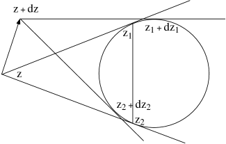
Figure 1: The Klein model

Resorting to Definition 2.3.1, we then have the

Theorem 2.4.1

Consider the hyperboloid $\mathcal{H}=\mathcal{S}\times\mathcal{S}-\Delta$ where the circle $\mathcal{S}$ has a projective structure defined by $\Phi\in\mathop{\mathrm{Diff}}\nolimits_{\mathrm{loc}}(\mathbb{R},\mathop{\mathbb{R}P^{1}\!}\nolimits)$ as in (2.8) or (2.9). Then, $\mathcal{H}$ carries a natural $\mathop{\mathrm{PSL}(2,\mathbb{R})}\nolimits$-invariant metric of the form

$$\mathop{\textrm{\rm g}}\nolimits_{1}=(\Phi\times\Phi)^{*}\frac{4\,dt_{1}dt_{2}}{(t_{1}-t_{2})^{2}}.$$ (2.12)

Proof: The cross-ratio (2.10) is $\mathop{\mathrm{PSL}(2,\mathbb{R})}\nolimits$-invariant and so is the Lorentz metric $4dt_{1}dt_{2}/(t_{1}-t_{2})^{2}$ of $\mathop{\mathbb{R}P^{1}\!}\nolimits\times\mathop{\mathbb{R}P^{1}\!}\nolimits-\Delta$ given by (2.11) with $z_{j}=t_{j}$ (see (2.9)). In any cases (2.8) or (2.9), the metric (2.12) defined on $\mathbb{R}^{2}-\Gamma$ where $\Gamma=(\Phi\times\Phi)^{-1}(\Delta)$ is automatically $\pi_{1}(\mathcal{S})$-invariant thanks to (2.7). It is invariant, as well, under the universal covering $\mathop{\mathrm{\widetilde{PSL}}(2,\mathbb{R})}\nolimits$ of $\mathop{\mathrm{PSL}(2,\mathbb{R})}\nolimits$. Hence, this metric descends to $\mathcal{H}=\mathcal{S}\times\mathcal{S}-\Delta=\pi\times\pi(\mathbb{R}^{2}-\Gamma)$ where $\pi:\mathbb{R}\to\mathcal{S}$ is the universal covering map. The projected metric $\mathop{\textrm{\rm g}}\nolimits_{1}$ is then clearly $\mathop{\mathrm{PSL}(2,\mathbb{R})}\nolimits$-invariant.    

Example (2.4) corresponds to the developing maps (2.8); as for the first developing map in (2.9), it leads via (2.12) to the metric of the Klein model of Section 2.2 (see Figure 1).

3 The Schwarzian derivative

3.1 Osculating homography of a diffeomorphism

Let $\varphi:\mathop{\mathbb{R}P^{1}\!}\nolimits\longrightarrow\mathop{\mathbb{R}P^{1}\!}\nolimits$ be a diffeomorphism and let $t_{0}\in\mathop{\mathbb{R}P^{1}\!}\nolimits$. We want to find the homography $h\in\mathop{\mathrm{PGL}(2,\mathbb{R})}\nolimits$ that best approximates the diffeomorphism $\varphi$ at this point $t_{0}$.

Proposition 3.1.1

This homography $h$ exists and is unique. It is completely defined by the conditions

$$\hfil h(t_{0}) = \varphi(t_{0}),$$

$$\hfil h^{\prime}(t_{0}) = \varphi^{\prime}(t_{0}),$$

$$\hfil h^{\prime\prime}(t_{0}) = \varphi^{\prime\prime}(t_{0}).$$

The diffeomorphism $h^{-1}\circ\varphi$ has the $2$-jet of the identity at $t_{0}$. The difference between $h$ and $\varphi$ starts, hence, at the third order derivative. (See, e.g., [11].)

Definition 3.1.1

The Schwarzian derivative of $\varphi$ at the point $t_{0}$ is

$$S(\varphi)(t_{0}):=\left(h^{-1}\circ\varphi\right)^{\prime\prime\prime}(t_{0}).$$

The quantity $S(\varphi)(t_{0})$ measures how much does the diffeomorphism $\varphi$ differ from an homography at the point $t_{0}$. All projective information about $\varphi$ is encoded into the Schwarzian derivative. If we identify the real projective line with $\mathbb{R}\cup\{\infty\}$ by: $[x,y]\longmapsto t=y/x$, we obtain the classical formula:

$$S(\varphi)=\left({\varphi^{\prime\prime\prime}(t)\over\varphi^{\prime}(t)}-{3\over 2}{\varphi^{\prime\prime}(t)^{2}\over\varphi^{\prime}(t)^{2}}\right)dt^{2}.$$ (3.13)

The graph $\Gamma_{\varphi}$ of our diffeomorphism is a simple closed curve on $\mathop{\mathbb{R}P^{1}\!}\nolimits\times\mathop{\mathbb{R}P^{1}\!}\nolimits$.

Definition 3.1.2

The homography $h$ and its graph $\Gamma_{h}$ are respectively called the osculating homography and the osculating hyperbola of $\varphi$ at $t_{0}$.

3.2 The Schwarzian as a projective differential invariant

Theorem 3.2.1 ([12])

The Schwarzian derivative is a third-order complete differential invariant for the group of diffeomorphisms of the projective line.

More precisely, if $\varphi$ and $\psi$ are two diffeomorphisms of $\mathop{\mathbb{R}P^{1}\!}\nolimits$, then

$$S(\varphi)=S(\psi)\qquad\Leftrightarrow\qquad\exists A\in\mathop{\mathrm{PSL}(2,\mathbb{R})}\nolimits,\ \psi=A\circ\varphi.$$

Theorem 3.2.2 ([2, 17, 27, 28])

The Schwarzian $S$ given by (3.13) is a non trivial $1$-cocycle, i.e.,

$$S(\varphi\circ\psi)=\psi^{*}S(\varphi)+S(\psi)\qquad\forall\varphi,\psi\in\mathop{\mathrm{Diff}}\nolimits_{+}(\mathop{\mathbb{R}P^{1}\!}\nolimits),$$

on the group of orientation-preserving diffeomorphisms of $\mathop{\mathbb{R}P^{1}\!}\nolimits$ with values in the $\mathop{\mathrm{Diff}}\nolimits_{+}(\mathop{\mathbb{R}P^{1}\!}\nolimits)$-module of real quadratic differentials $\mathcal{Q}(\mathop{\mathbb{R}P^{1}\!}\nolimits)$ of of $\mathop{\mathbb{R}P^{1}\!}\nolimits$. Its kernel is $\mathop{\mathrm{PSL}(2,\mathbb{R})}\nolimits$.

Remark 3.2.1

The Schwarzian cocycle (3.13) is uniquely characterized (up to a constant factor) by the property of having kernel $\mathop{\mathrm{PSL}(2,\mathbb{R})}\nolimits$.

3.3 Cartan formula of the cross-ratio

A useful means for calculating the Schwarzian derivative of a smooth map of the projective line is given by

Theorem 3.3.1 ([4])

Consider a smooth map $\varphi:\mathbb{R}P^{1}\longrightarrow\mathbb{R}P^{1}$ and four points $t_{1},\ldots,t_{4}\in\mathbb{R}P^{1}$ tending to $t\in\mathbb{R}P^{1}$; putting $\tau_{j}=\varphi(t_{j})$ one has

$$\frac{(\tau_{1},\tau_{2},\tau_{3},\tau_{4})}{(t_{1},t_{2},t_{3},t_{4})}-1=\frac{1}{6}S(\varphi)(t)(t_{1}-t_{2})(t_{3}-t_{4})+\hbox{\rm[higher order terms]}$$ (3.14)

where $S(\varphi)$ denotes the Schwarzian derivative (3.13) of $\varphi$.

This expression still makes sense for any smooth map of the circle $\mathcal{S}$ endowed with some projective structure given, for example, by (2.8) or (2.9). We, indeed, have the

Definition 3.3.1

Let $\varphi:\mathcal{S}\longrightarrow\mathcal{S}$ be a smooth map identified with one of its representatives in $C^{\infty}_{\pi_{1}(\mathcal{S})}(\mathbb{R})$, then the Schwarzian of $\varphi$ is the pull-back of the Schwarzian (3.14) of the induced map $\tilde{\varphi}$ of $\mathop{\mathbb{R}P^{1}\!}\nolimits$, namely

$$\mathbf{S}(\varphi)=\Phi^{*}S(\tilde{\varphi}).$$ (3.15)

We note that (3.15) yields a well-defined quadratic differential on $\mathcal{S}$ since one trivially finds $a^{*}\mathbf{S}(\varphi)=\mathbf{S}(\varphi)$ in view of $T(a)^{*}S(\tilde{\varphi})=S(\tilde{\varphi})$ for all $a\in\pi_{1}(\mathcal{S})\cong\mathbb{Z}$.

Proposition 3.3.1

One has, locally,

$$\mathbf{S}(\varphi)=S(\varphi)+\varphi^{*}S(\Phi)-S(\Phi).$$ (3.16)

Proof: Using $\tilde{\varphi}\circ\Phi=\Phi\circ\varphi$, one easily finds $\Phi^{*}S(\tilde{\varphi})(\theta)=S(\varphi)(\theta)+S(\Phi)(\varphi(\theta))\,\varphi^{\prime}(\theta)^{2}-S(\Phi)(\theta)$.    

4 Conformal transformations

4.1 Conformal Lorentz structures

Let us recall some basic definitions and facts about $2$-dimensional Lorentzian conformal geometry.

Definition 4.1.1 ([21])

A conformal Lorentz structure on a surface $\Sigma$ is characterized by a pair of transverse foliations; in other words, it is given by a splitting

$$T\Sigma=T_{1}\Sigma\oplus{}T_{2}\Sigma$$ (4.17)

into two trivial line bundles (light-cone field). We call $N_{1}$ and $N_{2}$, respectively, the spaces of leaves of the two foliations of $\Sigma$.

The leaves composing the “grid” associated to these foliations are, locally, given by

$$N_{1}:\theta_{1}=\mathop{\mathrm{missing}}{const.}\nolimits,\qquad N_{2}:\theta_{2}=\mathop{\mathrm{missing}}{const.}\nolimits$$

The conformal structure is characterized by the global intersection properties of the (null) leaves of $N_{1}$ and $N_{2}$.

One can associate to the splitting (4.17) a class of metrics on $\Sigma$, locally, of the form $\mathop{\textrm{\rm g}}\nolimits=F(\theta_{1},\theta_{2})\,d\theta_{1}d\theta_{2}$ where $F$ is some smooth positive function. If $\mathop{\textrm{\rm g}}\nolimits$ is any metric with prescribed null cone field $T_{1}\Sigma\oplus{}T_{2}\Sigma$, we denote by

$$\big{[}\mathop{\textrm{\rm g}}\nolimits\big{]}=\{F\cdot\mathop{\textrm{\rm g}}\nolimits|F\in{}C^{\infty}(\Sigma,\mathbb{R}^{+}_{*})\}$$ (4.18)

the class of metrics conformally equivalent to $\mathop{\textrm{\rm g}}\nolimits$. Thus, a conformal Lorentz structure [32] on $\Sigma$ is equivalently defined by $(\Sigma,\big{[}\mathop{\textrm{\rm g}}\nolimits\big{]})$.

Definition 4.1.2

A diffeomorphism $\varphi$ of $(\Sigma,\mathop{\textrm{\rm g}}\nolimits)$ is called conformal—we write $\varphi\in\mathop{\rm Conf}\nolimits(\Sigma,\mathop{\textrm{\rm g}}\nolimits)$—if

$$\varphi^{*}\!\mathop{\textrm{\rm g}}\nolimits=f_{\varphi}\cdot{\mathop{\textrm{\rm g}}\nolimits}\quad\mbox{for some\ }f_{\varphi}\in{}C^{\infty}(\Sigma,\mathbb{R}^{+}_{*}).$$ (4.19)

The function $f_{\varphi}$ is called the conformal factor associated with $\varphi$.

Remark 4.1.1

Definition 4.1.2 is general and holds in the Riemannian case. It is, for instance, well known that $\mathop{\rm Conf}\nolimits(H^{2})=\mathop{\mathrm{PSL}(2,\mathbb{R})}\nolimits$. In the Lorentzian case, the conformal group of $H^{1,1}$ is, however, infinite dimensional; more precisely, we will see that $\mathop{\rm Conf}\nolimits(H^{1,1})=\mathop{\mathrm{Diff}}\nolimits(\mathbb{T})$.

4.2 Conformal geometry of the Lorentz hyperboloid

We have seen (2.6) that the global intersection properties of the rulings of the hyperboloid yield (see Figure 2)

$$H=\mathbb{T}\times\mathbb{T}-\Delta$$ (4.20)

Figure 2: The hyperboloid

whose metric (2.4,2.11) is given by

$$\mathop{\textrm{\rm g}}\nolimits_{1}=\frac{4\,d\theta_{1}d\theta_{2}}{\left|e^{i\theta_{1}}-e^{i\theta_{2}}\right|^{2}}.$$ (4.21)

In view of the previous definitions 4.1.1 and 4.1.2, any conformal (grid-preserving) diffeomorphism $\varphi$ of a Lorentz surface $(\Sigma,\mathop{\textrm{\rm g}}\nolimits)$ is, locally, of the form $\varphi_{1}\times\varphi_{2}$ where $\varphi_{j}\in\mathop{\mathrm{Diff}}\nolimits(N_{j})$. A (global) conformal diffeomorphism of $\Sigma$ must preserve the two foliations by lines.

In our case, such a transformation of $\mathbb{T}^{2}-\Delta$ must preserve not only the meridians and parallels of $\mathbb{T}^{2}$, but the diagonal $\Delta$ as well. Therefore, $\varphi_{1}(\theta)=\varphi_{2}(\theta)$ for all $\theta\in\mathbb{T}$, whence the

Proposition 4.2.1 ([20])

There exists a canonical isomorphism

$$\mathop{\mathrm{Diff}}\nolimits(\Delta)\stackrel{{\scriptstyle\cong}}{{\longrightarrow}}\mathop{\rm Conf}\nolimits(H)$$

given by the diagonal map: $\varphi\longmapsto\varphi\times\varphi$.

Let us recall the

Theorem 4.2.1 ([20])

(i) Let $\varphi\in\mathop{\mathrm{Diff}}\nolimits_{+}(\mathbb{T})\cong\mathop{\rm Conf}\nolimits_{+}(H)$ be given. Then $f_{\varphi}=(\varphi^{*}\!\mathop{\textrm{\rm g}}\nolimits_{1})/\mathop{\textrm{\rm g}}\nolimits_{1}\longrightarrow 1$ as one tends to the conformal boundary $\Delta$.

(ii) The conformal factor $f_{\varphi}$ extends smoothly to $H\cup\Delta=\mathbb{T}^{2}$ and has, moreover, $\Delta$ as its critical set.

(iii) One has $\mathop{\mathrm{Hess}}\nolimits(f_{\varphi})|\Delta=\frac{1}{3}\widetilde{S}(\varphi)$ where

$$\widetilde{S}(\varphi)=S(\varphi)+\frac{1}{2}\left(\varphi^{\prime}(\theta)^{2}-1\right)d\theta^{2}.$$ (4.22)

(iv) The Schwarzian $\widetilde{S}(\varphi)$ completely determines $f_{\varphi}$.

Our proof proceeds as follows. Comparison with the definition (2.11) of the metric $\mathop{\textrm{\rm g}}\nolimits_{1}$ on the hyperboloid $H$ in terms of the cross-ratio prompts the following computation. Given any $\varphi\in\mathop{\mathrm{Diff}_{+}}\nolimits(\mathbb{T})$ viewed as a conformal diffeomorphism (4.19) of $(H,\mathop{\textrm{\rm g}}\nolimits_{1})$, apply the Cartan formula (3.14) in the case of a diffeomorphism of the circle $\mathbb{T}$, and get

$$\frac{(\varphi^{*}\!\mathop{\textrm{\rm g}}\nolimits_{1})(\theta_{1},\theta_{2})}{\mathop{\textrm{\rm g}}\nolimits_{1}(\theta_{1},\theta_{2})}-1 = f_{\varphi}(\theta_{1},\theta_{2})-1$$ (4.23)

$$= \frac{1}{6}S(\tilde{\varphi})(e^{i\theta})\left(e^{i\theta_{1}}-e^{i\theta_{2}}\right)^{2}+\cdots$$ (4.24)

where $\tilde{\varphi}(e^{i\theta})=e^{i\varphi(\theta)}$ and $\theta_{j}\longrightarrow\theta$ for $j=1,2$. A tedious calculation using (3.14) leads to

Lemma 4.2.1

If $\tilde{\varphi}\in\mathop{\mathrm{Diff}_{+}}\nolimits(\mathbb{T})$ is represented by $\varphi\in\mathop{\mathrm{Diff}}\nolimits_{2\pi\mathbb{Z}}(\mathbb{R})$, one has

$$S(\tilde{\varphi})(e^{i\theta})=-\left(S(\varphi)(\theta)+\frac{1}{2}\left(\varphi^{\prime}(\theta)^{2}-1\right)\right)e^{-2i\theta}.$$ (4.25)

From (4.23)–(4.25) one obtains

$$f_{\varphi}(\theta_{1},\theta_{2})-1=\frac{1}{6}\left(S(\varphi)(\theta)+\frac{1}{2}\left(\varphi^{\prime}(\theta)^{2}-1\right)\right)(\theta_{1}-\theta_{2})^{2}+\cdots$$ (4.26)

that is, theorem 1 in [20]. In particular, the conformal factor $f_{\varphi}$ extends to the diagonal $\Delta\subset\mathbb{T}^{2}$ (its critical set) and $f_{\varphi}|\Delta=1$, its transverse Hessian being related to the modified Schwarzian derivative (see (4.26)) by $\mathop{\mathrm{Hess}}\nolimits(f_{\varphi})=\frac{1}{3}\widetilde{S}(\varphi)$. The fourth item of theorem 4.2.1 will be a consequence of Theorem 5.1.2.

We are thus led to the

Theorem 4.2.2

(i) Given any $\varphi\in\mathop{\rm Conf}\nolimits_{+}(H)$ of $H=\mathbb{T}^{2}-\Delta$ and $c\neq 0$, the twice-symmetric tensor field $\varphi^{*}\!\mathop{\textrm{\rm g}}\nolimits_{c}-\mathop{\textrm{\rm g}}\nolimits_{c}$ of $H$ extends to null infinity $\Delta$ and defines a non trivial $1$-cocycle

$$S_{c}:\varphi\longmapsto\frac{3}{2}\left(\varphi^{*}\!\mathop{\textrm{\rm g}}\nolimits_{c}-\mathop{\textrm{\rm g}}\nolimits_{c}\right)\!|\Delta$$ (4.27)

of $\mathop{\mathrm{Diff}_{+}}\nolimits(\mathbb{T})$ with values in the module $\mathcal{Q}(\mathbb{T})$ of quadratic differentials of the circle, given by the (modified) Schwarzian derivative (4.22):

$$S_{c}=c\,\widetilde{S}.$$ (4.28)

(ii) There holds $H^{1}(\mathop{\mathrm{Diff}_{+}}\nolimits(\mathbb{T}),\mathcal{Q}(\mathbb{T}))=\mathbb{R}\left[S_{1}\right]$.

Proof: From the formulæ (4.26) and (4.21) one immediately gets

$$\left(\varphi^{*}\!\mathop{\textrm{\rm g}}\nolimits_{1}-\mathop{\textrm{\rm g}}\nolimits_{1}\right)|\Delta = \left({\textstyle\frac{2}{3}}\,\widetilde{S}(\varphi)(\theta)(\theta_{1}-\theta_{2})^{2}d\theta_{1}d\theta_{2}|e^{i\theta_{1}}-e^{i\theta_{2}}|^{-2}+\cdots\right)\!\Big{|}\Delta$$

$$= \left({\textstyle\frac{2}{3}}\,\widetilde{S}(\varphi)(\theta)d\theta_{1}d\theta_{2}+\cdots\right)\!\Big{|}\Delta$$

$$= \frac{2}{3}\,\widetilde{S}(\varphi)(\theta)\,d\theta^{2}$$

$$= \frac{2}{3}\,\widetilde{S}(\varphi).$$

Then (4.28) is clear by (2.4) and (2.5).

At last, part (ii) follows immediately from the knowledge that $H^{1}(\mathop{\mathrm{Diff}_{+}}\nolimits(\mathbb{T}),\mathcal{Q}(\mathbb{T}))$ is $1$-dimensional [9, 8] and generated by the class of the Schwarzian.    

Remark 4.2.1

The cocycle $\varphi\longmapsto\varphi^{*}\!\mathop{\textrm{\rm g}}\nolimits_{c}-\mathop{\textrm{\rm g}}\nolimits_{c}$ of $\mathop{\rm Conf}\nolimits_{+}(H)$ with values in the space of twice-covariant symmetric tensor fields is obviously trivial. Non triviality of the cocycle (4.27) quite remarkably stems from the “restriction” of the latter to null infinity $\Delta$.

Proposition 4.2.2

The group of direct isometries of the hyperboloid is

$$\mathop{\rm Isom}\nolimits_{+}(H,\mathop{\textrm{\rm g}}\nolimits_{c})=\ker(S_{c})\cong\mathop{\mathrm{PSL}(2,\mathbb{R})}\nolimits.$$ (4.29)

Proof: Using (4.27), we find that the group $\mathop{\rm Isom}\nolimits_{+}(H,\mathop{\textrm{\rm g}}\nolimits_{c})\subset\mathop{\mathrm{Diff}_{+}}\nolimits(\mathbb{T})$ of direct isometries is clearly a subgroup of $\ker({S_{c}})\cong\mathop{\mathrm{PSL}(2,\mathbb{R})}\nolimits$. Conversely, for any $\varphi\in\ker({S_{c}})$, and thanks to (4.24), the conformal factor in (4.23) is $f_{\varphi}=1$, i.e., $\varphi\in\mathop{\rm Isom}\nolimits_{+}(H,\mathop{\textrm{\rm g}}\nolimits_{c})$.    

Theorem 4.2.2 still holds true for the $\mathop{\mathrm{PSL}(2,\mathbb{R})}\nolimits$-invariant metric (2.12) on $\mathcal{S}\times\mathcal{S}-\Delta$. In fact, a calculation akin to that of (4.23,4.24) leads to

Proposition 4.2.3

Given any $\varphi\in\mathop{\rm Conf}\nolimits_{+}(\mathcal{H})$ of $\mathcal{H}=\mathcal{S}\times\mathcal{S}-\Delta$ where $\mathcal{S}$ is endowed with the projective structure (2.8) or (2.9), one has

$$\mathbf{S}(\varphi)=S_{1}(\varphi)=\frac{3}{2}\left(\varphi^{*}\!\mathop{\textrm{\rm g}}\nolimits_{1}-\mathop{\textrm{\rm g}}\nolimits_{1}\right)\!|\Delta$$ (4.30)

where the metric $\mathop{\textrm{\rm g}}\nolimits_{1}$ on $\mathcal{H}$ is given by (2.12) and the universal Schwarzian $\mathbf{S}$ by (3.15,3.16).

4.3 Conformal geometry of the flat cylinder

Let us envisage, for a moment, the flat induced Lorentz metric

$$\mathop{\textrm{\rm g}}\nolimits_{0}=d\theta_{1}d\theta_{2}$$ (4.31)

on the cylinder $H=\mathbb{T}^{2}-\Delta$. (A non significant constant factor might be introduced in the definition (4.31) of $\mathop{\textrm{\rm g}}\nolimits_{0}$.)

In this special case, the $\mathop{\mathrm{Diff}_{+}}\nolimits(\mathbb{T})$-cocycle $S_{0}$ defined, in the same manner as in (4.27), by

$$S_{0}(\varphi)=\left(\varphi^{*}\!\mathop{\textrm{\rm g}}\nolimits_{0}-\mathop{\textrm{\rm g}}\nolimits_{0}\right)|\Delta$$ (4.32)

is, plainly, a coboundary since $\mathop{\textrm{\rm g}}\nolimits_{0}$ admits a prolongation to $\Delta$. We, indeed, have $S_{0}(\varphi)(\theta)=(\varphi^{\prime}(\theta)^{2}-1)\,d\theta^{2}$. Notice that flatness of the metric is now related to triviality of the associated cocycle.

Proposition 4.3.1

The group of direct isometries of the flat cylinder is

$$\mathop{\rm Isom}\nolimits_{+}(H,\mathop{\textrm{\rm g}}\nolimits_{0})=\ker(S_{0})\cong\mathbb{T}.$$ (4.33)

Proof: Solving $\varphi^{*}\!\mathop{\textrm{\rm g}}\nolimits_{0}=\mathop{\textrm{\rm g}}\nolimits_{0}$ and $\varphi^{\prime}(\theta)>0$ gives $\varphi(\theta)=\theta+t$ with $t\in\mathbb{T}$, that is $\varphi\in\ker(S_{0})$.    

5 Symplectic structure on conformal classes of metrics on $\mathcal{S}\times\mathcal{S}-\Delta$

We analyze, in this section, the structure of the conformal classes of the previously introduced metrics $\mathop{\textrm{\rm g}}\nolimits_{c}$ and $\mathop{\textrm{\rm g}}\nolimits_{0}$ on the “hyperboloid” $\mathcal{H}$ and relate them to the generic coadjoint orbits [17] in the regular dual of the Virasoro group. It should be recalled that the conformal class of $\mathop{\textrm{\rm g}}\nolimits_{1}$ has first been identified with the homogeneous space $\mathop{\mathrm{Diff}_{+}}\nolimits(\mathbb{T})/\mathop{\mathrm{PSL}(2,\mathbb{R})}\nolimits$ in [19].

5.1 Homogeneous space $\mathop{\mathrm{Diff}_{+}}\nolimits(\mathcal{S})/\mathop{\mathrm{PSL}(2,\mathbb{R})}\nolimits$

5.1.1 Conformal classes of curved metrics

Consider first the curved case. If $c\neq 0$, denote by $M_{c}$ the space of metrics on $\mathcal{H}=\mathcal{S}\times\mathcal{S}-\Delta$ related to $\mathop{\textrm{\rm g}}\nolimits_{c}=c\,\mathop{\textrm{\rm g}}\nolimits_{1}$ (2.4) by a conformal diffeomorphism (see (4.18)), viz.

$$M_{c}=\{\mathop{\textrm{\rm g}}\nolimits\in\big{[}\mathop{\textrm{\rm g}}\nolimits_{1}\big{]}\,|\,\mathop{\textrm{\rm g}}\nolimits=\varphi^{*}\!\mathop{\textrm{\rm g}}\nolimits_{c},\varphi\in\mathop{\rm Conf}\nolimits_{+}(\mathcal{H})\}.$$

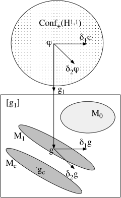
Figure 3: The conformal classes of metrics on $\mathbb{T}^{2}-\Delta$

These classes $M_{c}$ of metrics (see Figure 3) turn out to have a symplectic structure of their own.

Theorem 5.1.1

If $c\neq 0$, the homogeneous space

$$M_{c} = \mathop{\rm Im}\nolimits(\varphi\longmapsto\varphi^{*}\!\mathop{\textrm{\rm g}}\nolimits_{c})$$

$$\cong \mathop{\rm Conf}\nolimits_{+}(\mathcal{H})/\mathop{\rm Isom}\nolimits_{+}(\mathcal{H},\mathop{\textrm{\rm g}}\nolimits_{c})$$

is endowed with (weak) symplectic structure $\omega_{c}$ which reads

$$\omega_{c}(\delta_{1}\!\mathop{\textrm{\rm g}}\nolimits,\delta_{2}\!\mathop{\textrm{\rm g}}\nolimits)=\frac{3}{2}\int_{\Delta}{\!i_{\xi_{1}}L_{\xi_{2}}\!\mathop{\textrm{\rm g}}\nolimits}$$ (5.34)

where $\delta_{j}\!\mathop{\textrm{\rm g}}\nolimits=L_{\xi_{j}}\!\mathop{\textrm{\rm g}}\nolimits$ with $\xi_{j}\in\mathop{\rm Vect}\nolimits(\mathcal{S})$.

Proof: From (5.50) below, $\omega_{c}$ is, indeed, skew-symmetric in its arguments. It is, clearly, also closed. We then have $\delta_{2}\!\mathop{\textrm{\rm g}}\nolimits_{c}\in\ker\omega_{c}$ iff $\omega_{c}(\delta_{1}\!\mathop{\textrm{\rm g}}\nolimits_{c},\delta_{2}\!\mathop{\textrm{\rm g}}\nolimits_{c})=0$ for all $\xi_{1}\in\mathop{\rm Vect}\nolimits(\mathcal{S})$, i.e., iff $L_{\xi_{2}}\!\mathop{\textrm{\rm g}}\nolimits_{c}\!|\Delta=0$, that is iff $\delta_{2}\!\mathop{\textrm{\rm g}}\nolimits_{c}=0$ in view of (4.27) and (4.29).    

We will prove that $M_{c}$ is symplectomorphic to a Kirillov-Segal-Witten $\mathop{\mathrm{Diff}}\nolimits_{+}(\mathcal{S})$-orbit [17, 28, 34] for the affine coadjoint (anti-)action $\mathop{\rm Coad}\nolimits_{\Theta}$ on $\mathcal{Q}(\mathcal{S})$ defined by

$$\mathop{\rm Coad}\nolimits_{\Theta}(\varphi)q=\mathop{\rm Coad}\nolimits(\varphi)q+\Theta(\varphi)$$ (5.35)

where the $\mathop{\mathrm{Diff}}\nolimits_{+}(\mathcal{S})$-coadjoint (anti-)action reads

$$\mathop{\rm Coad}\nolimits(\varphi)q=\varphi^{*}q$$ (5.36)

and where $\Theta$, a $1$-cocycle of $\mathop{\mathrm{Diff}}\nolimits_{+}(\mathcal{S})$ with values in $\mathcal{Q}(\mathcal{S})$, is a particular Souriau cocycle [30].

5.1.2 Intermezzo

This technical section presents the standard $\mathop{\mathrm{Diff}_{+}}\nolimits(\mathcal{S})$-cocycles in a guise adapted to any projective structure (2.8,2.9) on the circle $\mathcal{S}$.

Consider the line element

$$\lambda=\Phi^{*}d\theta$$

on $\mathcal{S}$ associated with the developing map $\Phi\in\mathop{\mathrm{Diff}}\nolimits_{\mathrm{loc}}(\mathbb{R},\mathop{\mathbb{R}P^{1}\!}\nolimits)$. Actually, $\lambda$ is a $\pi_{1}(\mathcal{S})$-invariant line-element of $\mathbb{R}$ which therefore descends to $\mathcal{S}$.

Let $\varphi$ be a representative in $\mathop{\mathrm{Diff}}\nolimits_{\pi_{1}(\mathcal{S})}(\mathbb{R})$ of a diffeomorphism of $\mathcal{S}$ and let $\tilde{\varphi}=\Phi\circ\varphi\circ\Phi^{-1}$ denote the diffeomorphism it induces on $\mathop{\mathbb{R}P^{1}\!}\nolimits$.

Proposition 5.1.1

(i) The Euclidean cocycle $\mathbf{E}(\varphi)=\Phi^{*}E(\tilde{\varphi})$ where $E(\tilde{\varphi})=\log((\tilde{\varphi}^{*}d\theta)/d\theta)$ reads

$$\mathbf{E}(\varphi)=\log\left(\frac{\varphi^{*}\lambda}{\lambda}\right).$$ (5.37)

(ii) The affine cocycle $\mathbf{A}(\varphi)=\Phi^{*}dE(\tilde{\varphi})$ is then

$$\mathbf{A}(\varphi)=d\mathbf{E}(\varphi).$$ (5.38)

(iii) The Schwarzian cocycle $\mathbf{S}(\varphi)=\Phi^{*}S(\tilde{\varphi})$ (see (3.15,3.16)) retains the form

$$\mathbf{S}(\varphi)=\lambda\,d\left(\frac{\mathbf{A}(\varphi)}{\lambda}\right)-\frac{1}{2}\mathbf{A}(\varphi)^{2}.$$ (5.39)

Proof: We easily prove (iii) by noticing that the Schwarzian (3.13) can be written in term of the affine coordinate $\theta$ of $\mathop{\mathbb{R}P^{1}\!}\nolimits$ as

$$S(\tilde{\varphi})=d\theta\,d\left(\frac{\tilde{\varphi}^{\prime\prime}(\theta)}{\tilde{\varphi}^{\prime}(\theta)}\right)-\frac{1}{2}\left(\frac{\tilde{\varphi}^{\prime\prime}(\theta)}{\tilde{\varphi}^{\prime}(\theta)}\,d\theta\right)^{2}$$

and the affine cocycle as $A(\tilde{\varphi})=(\tilde{\varphi}^{\prime\prime}(\theta)/\tilde{\varphi}^{\prime}(\theta))\,d\theta$.    

For example, the $\mathop{\mathrm{Diff}_{+}}\nolimits(\mathbb{T})$-Schwarzian in angular coordinate is recovered with $\Phi$ as in (2.8); one finds

$$\mathbf{S}(\varphi)(\theta)=\widetilde{S}(\varphi)(\theta),$$

i.e., the modified Schwarzian derivative (4.22). See also [28].

Proposition 5.1.2

The infinitesimal Schwarzian takes either forms

$$\mathbf{s}(\xi)=s_{1}(\xi)$$

for any $\xi\in\mathop{\rm Vect}\nolimits(\mathcal{S})$ with

$$\mathbf{s}(\xi)=\lambda\,d\left(\frac{d\mathop{\rm Div}\nolimits\xi}{\lambda}\right)$$ (5.40)

and

$$s_{1}(\xi)=\mathop{{\textstyle{\frac{3}{2}}}}\nolimits{}\left(L_{\xi}\mathop{\textrm{\rm g}}\nolimits_{1}\right)\!|\Delta.$$

Proof: This follows clearly from (4.30) and (5.39).    

Remark 5.1.1

In local affine coordinate on $\mathop{\mathbb{R}P^{1}\!}\nolimits$, the infinitesimal Schwarzian (5.40) of $\xi=\xi(t)\partial/\partial{t}$ retains the familiar form

$$\mathbf{s}(\xi)=\xi^{\prime\prime\prime}(t)\,dt^{2}.$$

5.1.3 A Virasoro orbit

With these preparations, let us formulate the

Proposition 5.1.3

Endow $\mathop{\mathrm{Diff}}\nolimits_{+}(\mathcal{S})$ with the $1$-form $\alpha$ defined by

$$\alpha(\delta\varphi)=\frac{1}{2}\int_{\mathcal{S}}{\!\mathbf{A}(\varphi)\delta{}\mathbf{E}(\varphi)}$$ (5.41)

where $\delta\varphi=\delta(\varphi\circ\psi)$ with $\delta\psi=\xi\in\mathop{\rm Vect}\nolimits(\mathcal{S})$ at $\psi=\mathop{\mathrm{id}}\nolimits$.

(i) The exterior derivative of $\alpha$ is given, for $\xi_{1},\xi_{2}\in\mathop{\rm Vect}\nolimits(\mathcal{S})$, by

$$d\alpha(\delta_{1}\varphi,\delta_{2}\varphi)=\int_{\mathcal{S}}{\!\mathbf{S}(\varphi)([\xi_{1},\xi_{2}])}+\underbrace{\int_{\mathcal{S}}{\!d(\mathop{\rm Div}\nolimits\xi_{1})\,\mathop{\rm Div}\nolimits\xi_{2}}.}_{\mathop{\bf GF}\nolimits(\xi_{1},\xi_{2})}$$ (5.42)

(ii) If $\sigma$ denotes the canonical symplectic structure of the $\mathop{\mathrm{Diff}_{+}}\nolimits(\mathcal{S})$-affine coadjoint orbit $\mathcal{O}$ of the origin with Souriau cocycle $\mathbf{S}$ (see (5.35)), namely if

$$\mathcal{O} = \mathop{\rm Im}\nolimits(\mathbf{S})$$ (5.43)

$$\cong \mathop{\mathrm{Diff}_{+}}\nolimits(\mathcal{S}))/\mathop{\mathrm{PSL}(2,\mathbb{R})}\nolimits$$ (5.44)

then

$$d\alpha=\mathbf{S}^{*}\sigma.$$ (5.45)

Proof: Since $d\alpha(\delta_{1}\varphi,\delta_{2}\varphi)=\mathop{{\textstyle{\frac{1}{2}}}}\nolimits\int_{\mathcal{S}}{d(\delta_{1}\mathbf{E}(\varphi))\delta_{2}\mathbf{E}(\varphi)}-\mathop{{\textstyle{\frac{1}{2}}}}\nolimits\int_{\mathcal{S}}{d(\delta_{2}\mathbf{E}(\varphi))\delta_{1}\mathbf{E}(\varphi)}$ let us first remark that

$$\delta_{j}\mathbf{E}(\varphi)=\mathbf{A}(\varphi)(\xi_{j})+\mathop{\rm Div}\nolimits\xi_{j}$$

with the above notation. If we posit for convenience $a=\mathbf{A}/\lambda$, and note that $\lambda(\xi_{1})\mathop{\rm Div}\nolimits\xi_{2}-\lambda(\xi_{2})\mathop{\rm Div}\nolimits\xi_{1}=\lambda([\xi_{1},\xi_{2}])$, a lengthy calculation then leads to

$$d\alpha(\delta_{1}\varphi,\delta_{2}\varphi)=\int_{\mathcal{S}}{(da-\mathop{{\textstyle{\frac{1}{2}}}}\nolimits{}a^{2}\lambda)\lambda([\xi_{1},\xi_{2}])}+\int_{\mathcal{S}}{d(\mathop{\rm Div}\nolimits\xi_{1})\mathop{\rm Div}\nolimits\xi_{2}}.$$

Whence the sought equation (5.42).

Now, the affine coadjoint orbit of $q_{1}\in\mathcal{Q}(\mathcal{S})$ given by the action (5.35) carries a canonical symplectic structure $\sigma$ which reads [30]:

$$\sigma(\delta_{1}q,\delta_{2}q)=\langle{}q,[\xi_{1},\xi_{2}]\rangle+f(\xi_{1},\xi_{2})$$ (5.46)

at $q=\mathop{\rm Coad}\nolimits_{\Theta}(\varphi)q_{1}$; here $f\in{}Z^{2}(\mathop{\rm Vect}\nolimits(\mathcal{S}),\mathbb{R})$ is the derivative of the group-cocycle $\Theta\in{}Z^{1}(\mathop{\mathrm{Diff}_{+}}\nolimits(\mathcal{S}),\mathcal{Q}(\mathcal{S}))$ at the identity. The expression (5.42) of $d\alpha$ clearly matches that of $\sigma$ (5.46) with $q_{1}=0$, $\Theta=\mathbf{S}$ and $f=\mathop{\bf GF}\nolimits$ where the Gelfand-Fuchs cocycle [9] reads

$$\mathop{\bf GF}\nolimits(\xi_{1},\xi_{2})=-\int_{\mathcal{S}}{\!\mathbf{s}(\xi_{1})(\xi_{2})}$$ (5.47)

according to (5.40).    

Our main result is then given by

Theorem 5.1.2

The map

$$J_{c}:g\longmapsto\frac{3}{2}\left(\mathop{\textrm{\rm g}}\nolimits-\mathop{\textrm{\rm g}}\nolimits_{c}\right)\!\big{|}\Delta$$ (5.48)

establishes a symplectomorphism

$$J_{c}:(M_{c},\omega_{c})\longrightarrow(\mathcal{O}_{c},\sigma_{c})$$ (5.49)

between the metrics of $\mathcal{H}=\mathcal{S}\times\mathcal{S}-\Delta$ conformally related to $\mathop{\textrm{\rm g}}\nolimits_{c}$ and the affine coadjoint orbit $\mathcal{O}_{c}=c\cdot\mathcal{O}$ (see (5.44)) with central charge $c$, the inverse curvature (2.3).

Proof: Let us denote by $\mathop{\textrm{\rm g}}\nolimits_{c}:\mathop{\rm Conf}\nolimits_{+}(\mathcal{H})\longrightarrow{}M_{c}$ the orbital map and let us put $\mathop{\textrm{\rm g}}\nolimits=\mathop{\textrm{\rm g}}\nolimits_{c}(\varphi)=\varphi^{*}\!\mathop{\textrm{\rm g}}\nolimits_{c}$. We find, using (5.34),

$$\omega_{1}(\delta_{1}\!\mathop{\textrm{\rm g}}\nolimits,\delta_{2}\!\mathop{\textrm{\rm g}}\nolimits) = \mathop{{\textstyle{\frac{3}{2}}}}\nolimits\int_{\Delta}{\!i_{\xi_{1}}L_{\xi_{2}}(\mathop{\textrm{\rm g}}\nolimits-\mathop{\textrm{\rm g}}\nolimits_{1})}+\mathop{{\textstyle{\frac{3}{2}}}}\nolimits\int_{\Delta}{\!i_{\xi_{1}}L_{\xi_{2}}(\mathop{\textrm{\rm g}}\nolimits_{1})}$$

$$= \mathop{{\textstyle{\frac{3}{2}}}}\nolimits\int_{\Delta}{\!(\mathop{\textrm{\rm g}}\nolimits-\mathop{\textrm{\rm g}}\nolimits_{1})([\xi_{1},\xi_{2}])}+\mathop{{\textstyle{\frac{3}{2}}}}\nolimits\int_{\Delta}{\!i_{\xi_{1}}L_{\xi_{2}}(\mathop{\textrm{\rm g}}\nolimits_{1})}$$

$$= \int_{\Delta}{\!S_{1}(\varphi)([\xi_{1},\xi_{2}])}-\int_{\Delta}{\!s_{1}(\xi_{1})(\xi_{2})}$$

$$= \int_{\Delta}{\!\mathbf{S}(\varphi)([\xi_{1},\xi_{2}])}-\int_{\Delta}{\!\mathbf{s}(\xi_{1})(\xi_{2})}$$

with the help of Propositions 4.2.3 and 5.1.2. Note that we have taken into account the skew-symmetry of the Gelfand-Fuchs cocycle introduced in (5.42) and (5.47). One thus gets

$$\omega_{1}(\delta_{1}\!\mathop{\textrm{\rm g}}\nolimits,\delta_{2}\!\mathop{\textrm{\rm g}}\nolimits)=\langle\mathbf{S}(\varphi),[\xi_{1},\xi_{2}]\rangle+\mathop{\bf GF}\nolimits(\xi_{1},\xi_{2})$$ (5.50)

and, since $\mathop{\textrm{\rm g}}\nolimits_{c}=c\,\mathop{\textrm{\rm g}}\nolimits_{1}$,

$$\omega_{c}=c\,\omega_{1}.$$

Thanks to (5.42) and (5.45), one can claim that

$$d\alpha = \mathop{\textrm{\rm g}}\nolimits_{1}^{*}\omega_{1}$$

$$= \mathbf{S}^{*}\sigma.$$

At last, this clearly entails

$$\omega_{c}=J_{c}^{*}\sigma_{c}$$

where $\sigma_{c}=c\,\sigma$ is the canonical symplectic structure on $\mathcal{O}_{c}$.    

The following diagram summarizes our claim.

$$\matrix{\mathop{\rm Conf}\nolimits_{+}(\mathcal{H})&\smash{\mathop{\hbox to34.1433pt{\rightarrowfill}}\limits^{\scriptstyle\cong}}&\mathop{\mathrm{Diff}_{+}}\nolimits(\mathcal{S})\cr\hbox to0.0pt{\hss$\scriptstyle\mathop{\textrm{\rm g}}\nolimits_{c}$}\left\downarrow\vbox to17.07164pt{}\right.\hbox to0.0pt{$\scriptstyle$\hss}&&\hbox to0.0pt{\hss$\scriptstyle$}\left\downarrow\vbox to17.07164pt{}\right.\hbox to0.0pt{$\scriptstyle c\,\mathbf{S}$\hss}\cr M_{c}&\smash{\mathop{\hbox to34.1433pt{\rightarrowfill}}\limits^{\scriptstyle\cong}_{\scriptstyle J_{c}}}&\mathcal{O}_{c}\cr}$$

5.2 Homogeneous space $\mathop{\mathrm{Diff}_{+}}\nolimits(\mathcal{S})/\mathbb{T}$

Consider then the flat case (4.31) and introduce the space $M_{0}$ of metrics (see Figure 3) on $\mathcal{H}=\mathcal{S}\times\mathcal{S}-\Delta$ related to $\mathop{\textrm{\rm g}}\nolimits_{0}$ by a conformal diffeomorphism, viz.

$$M_{0}=\{\mathop{\textrm{\rm g}}\nolimits\in\big{[}\mathop{\textrm{\rm g}}\nolimits_{1}\big{]}\,|\,\mathop{\textrm{\rm g}}\nolimits=\varphi^{*}\!\mathop{\textrm{\rm g}}\nolimits_{0},\varphi\in\mathop{\rm Conf}\nolimits_{+}(\mathcal{H})\}.$$

Theorem 5.2.1

The homogeneous space

$$M_{0} = \mathop{\rm Im}\nolimits(\varphi\longmapsto\varphi^{*}\!\mathop{\textrm{\rm g}}\nolimits_{0})$$

$$\cong \mathop{\rm Conf}\nolimits_{+}(\mathcal{H})/\mathop{\rm Isom}\nolimits_{+}(\mathcal{H},\mathop{\textrm{\rm g}}\nolimits_{0})$$

is endowed with a (weak) symplectic structure $\omega_{0}$ which reads

$$\omega_{0}(\delta_{1}\!\mathop{\textrm{\rm g}}\nolimits,\delta_{2}\!\mathop{\textrm{\rm g}}\nolimits) = \int_{\Delta}{\!i_{\xi_{1}}L_{\xi_{2}}\!\mathop{\textrm{\rm g}}\nolimits}$$ (5.51)

$$= \int_{\Delta}{\!\!\mathop{\textrm{\rm g}}\nolimits([\xi_{1},\xi_{2}])}$$ (5.52)

where $\delta_{j}\!\mathop{\textrm{\rm g}}\nolimits=L_{\xi_{j}}\!\mathop{\textrm{\rm g}}\nolimits$ with $\xi_{j}\in\mathop{\rm Vect}\nolimits(\mathcal{S})$.

Proof: Since $\mathop{\textrm{\rm g}}\nolimits_{0}$ can be prolongated to $\Delta$, (5.51) may be rewritten as (5.52) which is manifestly skew-symmetric in its arguments. The closed $2$-form $\omega_{0}$ is weakly non degenerate as $\delta_{2}\!\mathop{\textrm{\rm g}}\nolimits\in\ker\omega_{0}$ iff $L_{\xi_{2}}\!\mathop{\textrm{\rm g}}\nolimits\!|\Delta=0$, i.e. $\delta_{2}\!\mathop{\textrm{\rm g}}\nolimits=0$ in view of (4.32) and (4.33).    

In fact, $M_{0}$ is symplectomorphic to a $\mathop{\mathrm{Diff}_{+}}\nolimits(\mathcal{S})$-coadjoint orbit [17] as shown below.

Let us consider the following quadratic differential

$$q_{0}=\mathop{\textrm{\rm g}}\nolimits_{0}\!|\Delta\in\mathcal{Q}(\mathcal{S})$$ (5.53)

so that the $\mathop{\mathrm{Diff}_{+}}\nolimits(\mathcal{S})$-coadjoint (anti-)action $\mathop{\rm Coad}\nolimits$ given by (see (5.36)) $\mathop{\rm Coad}\nolimits(\varphi):q_{0}\longmapsto{}q=\varphi^{*}q_{0}$, reads according to (4.32):

$$q=q_{0}+S_{0}(\varphi).$$ (5.54)

Proposition 5.2.1

Endow $\mathop{\mathrm{Diff}}\nolimits_{+}(\mathcal{S})$ with the $1$-form $\alpha_{0}$ defined by

$$\alpha_{0}(\delta\varphi)=-\int_{\mathcal{S}}{\!(\varphi^{*}q_{0})(\xi)}$$

where, again, $\delta\varphi=\delta(\varphi\circ\psi)$ with $\delta\psi=\xi\in\mathop{\rm Vect}\nolimits(\mathcal{S})$ at $\psi=\mathop{\mathrm{id}}\nolimits$.

(i) We have, for any $\xi_{1},\xi_{2}\in\mathop{\rm Vect}\nolimits(\mathcal{S})$,

$$d\alpha_{0}(\delta_{1}\varphi,\delta_{2}\varphi)=\int_{\mathcal{S}}{\!(\varphi^{*}q_{0})([\xi_{1},\xi_{2}])}.$$

(ii) The $\mathop{\mathrm{Diff}}\nolimits_{+}(\mathcal{S})$-coadjoint orbit through $q_{0}$ (5.53) is

$$\mathcal{O}_{q_{0}} = \mathop{\rm Im}\nolimits(q_{0}\circ\mathop{\rm Ad}\nolimits)$$ (5.55)

$$\cong \mathop{\mathrm{Diff}}\nolimits_{+}(\mathcal{S})/\mathbb{T}$$ (5.56)

and is endowed with the symplectic $2$-form $\sigma_{0}$ such that

$$d\alpha_{0}=(q_{0}\circ\mathop{\rm Ad}\nolimits)^{*}\sigma_{0}.$$

Proof: If $\delta_{j}\varphi$ is associated with $\xi_{j}\in\mathop{\rm Vect}\nolimits(\mathcal{S})$ at $\varphi\in\mathop{\mathrm{Diff}_{+}}\nolimits(\mathcal{S})$, one readily finds $\delta_{j}q=L_{\xi_{j}}q$ and $d\alpha_{0}(\delta_{1}\varphi,\delta_{2}\varphi)=-\alpha_{0}([\delta_{1},\delta_{2}]\varphi)=\langle{}q,[\xi_{1},\xi_{2}]\rangle$ which descends as the canonical symplectic $2$-form $\sigma_{0}$ of $\mathcal{O}_{q_{0}}$, namely

$$d\alpha_{0}(\delta_{1}\varphi,\delta_{2}\varphi)=\sigma_{0}(\delta_{1}q,\delta_{2}q).$$

We then simply check that $\ker(d\alpha_{0})$ is $1$-dimensional and integrated by $\ker(S_{0})\cong\mathbb{T}$ (see (4.33) and (5.54)).    

The “flat” counterpart of Theorem 5.1.2 is now at hand.

Theorem 5.2.2

The map

$$J_{0}:\mathop{\textrm{\rm g}}\nolimits\longmapsto\mathop{\textrm{\rm g}}\nolimits\big{|}\Delta$$ (5.57)

establishes a symplectomorphism

$$J_{0}:(M_{0},\omega_{0})\longrightarrow(\mathcal{O}_{q_{0}},\sigma_{0})$$ (5.58)

between the metrics of $\mathcal{H}=\mathcal{S}\times\mathcal{S}-\Delta$ conformally related to $\mathop{\textrm{\rm g}}\nolimits_{0}$ and the coadjoint orbit $\mathcal{O}_{q_{0}}$ (see 5.56) with zero central charge.

Proof: Clear.    

5.3 Bott-Thurston cocycle and contactomorphisms

It is know since the work of Kirillov [17] that the $\mathop{\mathrm{Diff}_{+}}\nolimits(\mathcal{S})$-homogeneous spaces we dealt with in Sections 5.1 and 5.2 are, in fact, genuine coadjoint orbits of the Virasoro group, $\mathop{\rm Vir}\nolimits$, i.e., the $(\mathbb{R},+)$-central extension [31] of $\mathop{\mathrm{Diff}_{+}}\nolimits(\mathcal{S})$ that can be recovered as follows in our setting.

Let us emphasize that the $1$-form $\alpha$ (5.41) on $\mathop{\mathrm{Diff}}\nolimits_{+}(\mathcal{S})$ fails to be invariant. So, let us equip $\mathop{\mathrm{Diff}}\nolimits_{+}(\mathcal{S})\times\mathbb{R}$ with the following “contact” $1$-form $\widehat{\alpha}$, viz.

$$\widehat{\alpha}(\delta\varphi,\delta{t})=\alpha(\delta\varphi)+\delta{t}.$$ (5.59)

Now, the $2$-form $d\widehat{\alpha}$ is $\mathop{\mathrm{Diff}}\nolimits_{+}(\mathcal{S})$-invariant and plainly descends to $M_{1}$ as $\omega_{1}$ (see (5.45) and (5.48,5.49)). We now have the

Proposition 5.3.1

Lifting $\mathop{\mathrm{Diff}}\nolimits_{+}(\mathcal{S})$ into the group of automorphisms of $(\mathop{\mathrm{Diff}}\nolimits_{+}(\mathcal{S})\times\mathbb{R},\widehat{\alpha})$ yields the Virasoro group $\mathop{\rm Vir}\nolimits$ with multiplication law

$$(\varphi_{1},t_{1})\cdot(\varphi_{2},t_{2})=\Big{(}\varphi_{1}\circ\varphi_{2},t_{1}+t_{2}\underbrace{-\frac{1}{2}\int_{\mathcal{S}}{\!\mathbf{E}(\varphi_{1}\circ\varphi_{2})\mathbf{A}(\varphi_{2})}}_{\mathop{\bf BT}\nolimits(\varphi_{1},\varphi_{2})}\Big{)}$$ (5.60)

where $\mathop{\bf BT}\nolimits$ is the Bott-Thurston cocycle [2] of $\mathop{\mathrm{Diff}_{+}}\nolimits(\mathcal{S})\cong\mathop{\rm Conf}\nolimits_{+}(\mathcal{H})$.

Proof: Using the cocycle relation $\mathbf{E}(\varphi\circ\psi)=\psi^{*}\mathbf{E}(\varphi)+\mathbf{E}(\psi)$—see (5.37)—and (5.38,5.41), one immediately finds

$$\alpha(\delta(\varphi\circ\psi)) = \mathop{{\textstyle{\frac{1}{2}}}}\nolimits\int_{\mathcal{S}}{\!\psi^{*}(\mathbf{A}(\varphi)\delta(\mathbf{E}(\varphi))}+\mathop{{\textstyle{\frac{1}{2}}}}\nolimits\int_{\mathcal{S}}{\!\mathbf{A}(\psi)\delta(\mathbf{E}(\varphi\circ\psi))}$$

$$= \alpha(\delta\varphi)+\delta\left[\mathop{{\textstyle{\frac{1}{2}}}}\nolimits\int_{\mathcal{S}}{\!\mathbf{E}(\varphi\circ\psi)\mathbf{A}(\psi)}\right]$$

for all $\varphi,\psi\in\mathop{\mathrm{Diff}_{+}}\nolimits(\mathcal{S})$. Looking for those maps $(\varphi,t)\longmapsto(\varphi^{\star},t^{\star})$ such that $\varphi^{\star}=\varphi\circ\psi$ and $\widehat{\alpha}(\delta\varphi^{\star},\delta{t^{\star}})=\widehat{\alpha}(\delta\varphi,\delta{t})$ leads to $t^{\star}=t+\mathop{\bf BT}\nolimits(\varphi,\psi)+\mathop{\mathrm{missing}}{const.}\nolimits$, hence, to the group law (5.60).    

The triple $(\mathbf{S},\mathop{\bf GF}\nolimits,\mathop{\bf BT}\nolimits)$ is a special instance of a general structure that has been coined “trilogy of the moment” [16].

Remark 5.3.1

It would be interesting to have a conformal interpretation of the contact structure $\mathop{\rm Vir}\nolimits/(\ker\widehat{\alpha}\cap\ker{d\widehat{\alpha}})$ above $(M_{1},\omega_{1})$.

6 Conclusion and outlook

This work prompts a series of more or less ambitious questions connected with the striking analogies between conformal geometry of Lorentz surfaces and projective geometry of conformal infinity that we have just discussed. It constitutes an introduction to a more detailed paper (in preparation) where the authors wish to tackle the following problems.

1. Is it possible to realize any Virasoro coadjoint orbit as a conformal class of Lorentz metrics on the cylinder? If this is so, spell out the symplectic forms in terms of the classes of metrics; also study the relationship between the properties of an orbit and the dynamics of the null foliations in the associated conformal class. There exists, in fact, a map sending the space of Virasoro orbits—modules of projective structures on the circle—to the space of modules of Lorentzian conformal structures on the cylinder; analyze its properties. More conceptually, given a conic $C$ in the real projective plane, what are the links between the space of projective structures on $C$, the space of Lorentzian structures in the exterior of $C$ and the space of Riemannian metrics in the interior of $C$?

2. The Ghys theorem [10, 24] states that any diffeomorphism of the projective line has at least four points where its Schwarzian vanishes, i.e., four points where the contact of the graph of the diffeomorphism with its osculating hyperbola is greater than the generic one. This result is a Lorentzian analogue of the so-called four vertices theorem for closed curves in the Euclidean plane. In our context, the Ghys theorem would imply the existence, for any conformal automorphism of the hyperboloid, of some particular points where this diffeomorphism is closer than usual to an isometry.

3. The orbit $\mathop{\mathrm{Diff}}\nolimits(\mathbb{T})/\mathop{\mathrm{PSL}(2,\mathbb{R})}\nolimits$ embeds symplectically in the universal Teichmüller space $T(1)=\mathop{\mathrm{QS}}\nolimits(\mathbb{T})/\mathop{\mathrm{PSL}(2,\mathbb{R})}\nolimits$, where $\mathop{\mathrm{QS}}\nolimits(\mathbb{T})$ denotes the group of quasi-symmetric homeomorphisms of the circle [23]. With the help of the quantum differential calculus of Connes, it is possible to construct extensions of the three fundamental cocycles $\mathbf{E}$, $\mathbf{A}$ and $\mathbf{S}$ to the group $\mathop{\mathrm{QS}}\nolimits(\mathbb{T})$ [22]. Can one construct a “quantum analogue” of the Lorentzian hyperboloid whose conformal class may be identified with $T(1)$?

Let us finally mention two other subjects closely connected with our problem, namely the geometry of the Wess-Zumino-Witten model [7] and Douglas’ proof of the Plateau problem revisited by Guillemin, Kostant and Sternberg [15].

References

- [1]
- [2] R. Bott, “On the characteristic classes of groups of diffeomorphisms” Enseign. Math., 23, 3-4 (1977) 209–220.
- [3] E. Cartan, “Sur les variétés à connexion projective”, Bull. Soc. Math. France, 52 (1924) 205–241.
- [4] E. Cartan, Leçons sur la théorie des espaces à connexion projective, Gauthiers-Villars, Paris (1937).
- [5] E. Cartan, Leçons sur la géométrie projective complexe, Gauthiers-Villars, Paris (1950).
- [6] E. Cech and G. Fubini, Introduction à la géométrie projective différentielle des surfaces, Gauthier-Villars, Paris (1931).
- [7] F. Falceto and K. Gawedski, “On quantum group symmetries of conformal field theories” Proceedings of the XXth International Conference on Differential Geometric Methods in Theoretical Physics, Vol. 1, 2 (New York, 1991), 972–985, World Sci. Publishing, River Edge, NJ (1992).
- [8] D.B. Fuks, Cohomology of infinite-dimensional Lie algebras, Consultants Bureau, New York (1987).
- [9] I.M. Gel’fand and D.B. Fuks, “The cohomologies of the Lie algebra of the vector fields in a circle”, Functional Anal. Appl. 2, 4 (1968) 342–343.
- [10] E. Ghys, “Cercles osculateurs et géométrie lorentzienne”, Colloquium talk, Journée inaugurale du CMI, Marseille (Février 1995).
- [11] E. Ghys, “Déformations de flots d’Anosov et de groupes fuchsiens”, Ann. Inst. Fourier 42, 1-2 (1992) 209–247.
- [12] M. Green, “The moving frame, differential invariants and rigidity theorems for curves in homogeneous spaces”, Duke Math. J. 45, 4 (1978) 735–779.
- [13] L. Guieu, “Stabilisateurs cycliques pour la représentation coadjointe du groupe des difféomorphismes du cercle”, Bull. Sci. Math. (to appear).
- [14] L. Guieu, “Nombre de rotation, structures géométriques sur un cercle et groupe de Bott-Virasoro”, Ann. Inst. Fourier 46, 4 (1996) 971–1009.
- [15] V. Guillemin, B. Kostant and S. Sternberg, “Douglas’ solution of the Plateau problem”, Proc. Natl. Acad. Sci. USA 85, 10 (1988) 3277–3278.
- [16] P. Iglesias, “La trilogie du moment”, Ann. Inst. Fourier 45, 3 (1995) 825–857.
- [17] A.A. Kirillov, “Infinite dimensional Lie groups: their orbits, invariants and representations. The geometry of moments”, Lecture Notes in Math. 970 Springer-Verlag (1982) 101–123.
- [18] A.A. Kirillov and D.V. Yuriev, “Kähler geometry of the infinite dimensional homogeneous space ”, Functional Anal. Appl. 21, 4 (1987) 284–294.
- [19] B. Kostant and S. Sternberg, “Symplectic reduction, BRS cohomology, and infinite-dimensional Clifford algebras”, Ann. Phys. (NY) 176 (1987) 49–113.
- [20] B. Kostant and S. Sternberg, “The Schwartzian derivative and the conformal geometry of the Lorentz hyperboloid” in Quantum theories and geometry, M. Cahen and M. Flato (Eds), 1988, 113–125.
- [21] R. Kulkarni, “An analogue of the Riemann mapping theorem for Lorentz metrics”, Proc. R. Soc. Lond. A 401 (1985) 117–130.
- [22] S. Nag and D. Sullivan, “Teichmüller theory and the universal period mapping via quantum calculus and the space on the circle”, Osaka J. Math. 32, 1 (1995) 1–34.
- [23] S. Nag and A. Verjovsky, “ and the Teichmüller spaces”, Comm. Math. Phys. 130 (1990) 123–138.
- [24] V.Yu. Ovsienko and S. Tabachnikov, “Sturm theory, Ghys theorem on zeroes of the Schwarzian derivative and flattening of Legendrian curves”, Selecta Math. (N.S.) 2, 2 (1996) 297–307.
- [25] R. Penrose, Techniques of differential topology in relativity, Society for Industrial and Applied Mathematics, Philadelphia (1972).
- [26] H. Poincaré, La science et l’hypothèse, Flammarion (1902).
- [27] C. Roger, “Extensions centrales d’algèbres et de groupes de Lie de dimension infinie, algèbre de Virasoro et généralisations”, Reports Math. Phys. 35, 2/3 (1995) 225–266.
- [28] G.B. Segal, “Unitary representations of some infinite dimensional groups”, Comm. Math. Phys. 80, 3 (1981) 301–342.
- [29] G.B. Segal, “The geometry of the KdV equation”, Proc. of the Trieste conf. on topological methods in QFT theory (June 1990) 96–106, W. Nahm et al. Eds, World Scientific.
- [30] J.-M. Souriau, Structure des systèmes dynamiques, Dunod (1970, ©1969). Structure of Dynamical Systems. A Symplectic View of Physics, translated by C.H. Cushman-de Vries (R.H. Cushman and G.M. Tuynman, Translation Editors), Birkhäuser (1997).
- [31] G.M. Tuynman and W.J. Wiegerinck, “Central extensions and physics”, J. Geom. Phys. 4 (1987), 207–258.
- [32] T. Weinstein, An introduction to Lorentz surfaces, Walter de Gruyter, Berlin, New York (1996).
- [33] E.J. Wilczynski, Projective differential geometry of curves and ruled surfaces, Teubner, Leipzig (1906).
- [34] E. Witten, “Coadjoint orbits of the Virasoro group”, Comm. Math. Phys. 114, 1 (1988) 1–53.
- [35] J. A. Wolf, Spaces of constant curvature, McGraw-Hill, New York (1967).