THE GASSNER REPRESENTATION

FOR STRING LINKS

Paul Kirk, Charles Livingston, and Zhenghan Wang

April 29, 1998

Abstract The Gassner representation of the pure braid group to $GL_{n}({\bf Z}[{\bf Z}^{n}])$ can be extended to give a representation of the concordance group of $n$-strand string links to $GL_{n}(F)$, where $F$ is the field of quotients of ${\bf Z}[{\bf Z}^{n}]$, $F={\bf Q}(t_{1},\cdots,t_{n})$; this was first observed by Le Dimet. Here we give a cohomological interpretation of this extension. Our first application is to prove that the representation is hermitian, extending a known result for braids. A simple proof of the concordance invariance of the represenation also follows. The cohomological approach leads to algorithms for computing the Gassner representation, and these in turn yield connections between the Gassner represention of a string link and the Alexander matrix of the link closure of that string link; a new factorization result for Alexander polynomials follows. A random walk, or probablistic, approach to the Gassner representation is given, extending previous work concerning the 1-variable Burau representation. We next show that by suitably normalizing, the Gassner matrix determines, and is determined by, finite type link invariants. The paper concludes with an interpretation of the determinant of the Gassner matrix in terms of Reidemeister torsion, yielding an alternative approach to the factorization of the Alexander polynomial.

THE GASSNER REPRESENTATION

FOR STRING LINKS

Paul Kirk, Charles Livingston, and Zhenghan Wang

April 29, 1998

1 Introduction

The correspondence between links and braids, as detailed by the Markov theorem, has made the study of representations of the braid group a topic of great interest in classical knot theory. Prior to the work of Jones [11], the most important such representation was the Burau representation and its generalization, the Gassner representation, a homomorphism defined on the pure braid group on $n$ strands, $P_{n}$:

$$\gamma:P_{n}\to GL_{n}({\bf Z}[{\bf Z}^{n}]).$$

A basic reference for the properties of the Burau and Gassner representations is [4]; more recent work investigating the Gassner representation includes [1, 6, 18, 19].

In studying links, as opposed to knots, it has often proved useful to move from the setting of braids to the more general objects of string links. A string link is simply a braid except that the strands are not required to be monotonic; see Figure 1 and later discussions for details. The usefulness of this approach is perhaps best exemplified in the work of Habegger and Lin [10] in which a link homotopy classification is achieved through the interplay between links and string links. Part of the usefulness of braids is that there is a natural group structure on the set of all braids, but there is no similar group structure on the set of string links. However, once a natural equivalence relation is placed on the set of string links, either string link homotopy or concordance, a natural group structure reappears.

A significant advance in the study of links occurred in the work of Le Dimet on link concordance. In [13] he observed that the Gassner representation extends to the group of concordance classes of string links provided one extends the range to $GL_{n}(F)$ where $F$ denotes the quotient field of ${\bf Z}[{\bf Z}^{n}]$. It is the purpose of this article to explore this extension. We present simple new perspectives on its definition, its computation, and its application to obtain both general results and interesting families of examples.

A completely different approach to exploring the Gassner representation of string links is being investigated by Ted Stanford. His work is now in preparation.

We thank Jim Davis , X. S. Lin, and Kent Orr for contributions to this work. In particular, Orr showed us the proof of Proposition 2.3. Davis helped us develop much of the work concerning torsion, presented in Section 10.

Contents

In Section 2 we construct the Gassner matrix of a string link; the argument uses a single straightforward cohomology computation. The definition is very simple and completely trivial in the case of braids. We were surprised that this definition does not seem to appear explicitly in the literature, even in the context of braids or the Burau representation.

The Burau and Gassner representations of braids are unitary with respect to a particular Hermitian form. This has been observed in [1, 21, 16]. In Section 3 we show that this symmetry extends to the case of the Gassner representation for string links. In addition, we show that the Hermitian form corresponds to Poincarè duality on an appropriate cohomology group.

In Section 4 we use the well-known relationship between cohomology and the Fox calculus to describe an algorithm for computing the Gassner representation of a string link in terms of a presentation of the fundamental group of its complement. This also sets up some linear algebra which proves useful in later sections.

In Section 5 we give the argument that the resulting extension of the Gassner representation is a concordance and even I-equivalence invariant of the string link. I-equivalence is the equivalence relation defined by non-locally flat concordance. (It can be shown that two links or string links are I-equivalent if and only if adding local knots to each can result in concordant objects.)

Section 6 contains our main results, exploring a simple relationship between the Gassner matrix of a string link and the Alexander matrix of its closure. We show that the Gassner matrix of a string link shares many formal properties with the Alexander matrix of a link and exploit this to define the Alexander function of a string link. In particular we prove that the Alexander polynomial of the closure of a string link can be factored as a product of a polynomial associated to the Gassner representation of the string link and a second polynomial representing a Reidemeister torsion naturally associated to the string link. This torsion invariant vanishes for braids and hence our result generalizes the classical result relating the Gassner matrix of a braid and the Alexander polynomial of the associated link [4]. (See also [19].) In Corollary 6.10 we show that the Alexander ideals $E_{k}(\hat{L})$ of the closure $\hat{L}$ of a pure string link $L$ link vanish if and only if the Gassner matrix $\gamma(L)$ has the eigenvalue $1$ with multiplicity $k$. In Theorem 6.11 we show that the 1-variable Alexander polynomials of the link closure of a string link $L$, $\hat{L}$, and the knot closure, $\widehat{LB}$, are related by the formula

$$\bar{\Delta}_{\hat{L}}=\bar{\Delta}_{\widehat{LB}}\cdot{{\det(I-\tilde{\beta}(L))}\over{{\det(I-\tilde{\beta}(L)\tilde{\beta}(B))}}}.$$

The knot closure, $\widehat{LB},$ is formed from the link closure by banding the components together in a natural way, described explicitly in Section 6. (The correction term $\det(I-\tilde{\beta}(L))/\det(I-\tilde{\beta}(L)\tilde{\beta}(B))$ is a string link I-equivalence invariant of $L$.)

Section 7 presents examples. For instance, we demonstrate that the subgroup of the concordance group of string links formed by braids is not a normal subgroup.

In Section 8 we describe an alternative approach to the Gassner representation via the notion of random walks on the string link. This generalizes similar work for the Burau representation developed in [15]. Using this approach we are able to describe a construction which, beginning with almost any string link, produces an infinite family of string links, none of which are concordant (or even I-equivalent) and all of which have the same closure as the original string link. We also indicate in this section that in some sense the Gassner representation is the most general representation that can be attained via this random walk approach.

Section 9 discusses the connection between the Gassner representation and finite type invariants. In particular, by suitably normalizing it is seen that the Gassner representation is made up of finite type invariants. A consequence is that it is determined by Milnor invariants of the string link, although no explicit connection has been identified.

Finally, in Section 10 we interpret some of the previous work, especially the product formula of Section 6, in terms of torsion invariants associated to a string link and its associated closure.

2 A cohomological definition of the Gassner representation

We begin by introducing notation which will be in force throughout this article. Let $n$ be a positive integer; usually $n$ denotes the number of components of a (string) link. We will denote by $\Lambda$ the integral group ring of ${\bf Z}^{n}$ which will be thought of as the ring of Laurent polynomials in the variables $t_{1},\cdots,t_{n}$, $\Lambda={\bf Z}[t_{1},t_{1}^{-1},\cdots,t_{n},t_{n}^{-1}]$. Its fraction field, ${\bf Q}(t_{t},\cdots,t_{n})$, is the field of rational functions in the $t_{i}$ and will be denoted by $F$. We will occasionally use the localization $\Lambda_{S}$ of $\Lambda$ obtained by inverting all elements in the set, $S$, of Laurent polynomials $f\in\Lambda$ satisfying $f(1,\cdots,1)=1$. Thus $\Lambda\subset\Lambda_{S}\subset F$. Note that the units in $\Lambda$ are elements of the form $\pm t_{1}^{a_{1}}\cdots t_{n}^{a_{n}}$.

The formal definition of a string link is as follows. Given a positive integer $n$, fix $n$ points in the interior of the 2-disk $p_{1},\cdots,p_{n}$ , say $p_{i}=(-1/(i+1),0)$. A string link of n components is a smooth, proper, oriented 1-dimensional submanifold of $D^{2}\times[0,1]$ homeomorphic to the disjoint union of $n$ intervals such that the initial point of each interval coincides with some $p_{i}\times\{0\}$ and the endpoint coincides with $p_{j}\times\{1\}$. In the figures the orientation is such that the components run from the bottom to the top of the diagrams.

Equivalently, one can think of a string link as a proper embedding of $n$ intervals, rather than as a submanifold. Figure 1 illustrates a 3-stranded string link.

Figure 1:

A pure string link of n components is a string link so that the component labeled $i$ has initial point $p_{i}\times\{0\}$ and endpoint $p_{i}\times\{1\}$.

Two string links are called isotopic if there is a smooth family of string links interpolating between the two.

Two string links are called concordant if there is a proper, locally flat, embedding of $n$ copies of $[0,1]\times[0,1]$ in $D^{2}\times[0,1]\times[0,1]$ restricting to the two string links when the last coordinate is $0$ or $1$, and mapping to the proper $\{p_{i}\}\times\{0,1\}\times[0,1]$ when the middle coordinate is $0$ or $1$.

Finally, two string links are called I-equivalent if we drop the requirement that the concordance be locally flat.

In this article we will simultaneously consider two situations which can be roughly formulated as the Gassner/multi-variable case and the Burau/one-variable case. The emphasis will be on the first case but for the most part everything we say applies in either case. However, the two cases operate on slightly different categories of string links. The proper context for the Gassner/multi-variable case is to use colored string links; these are string links so that each component is indexed with an integer in $\{1,\cdots,n\}$. For the Burau/single-variable case the coloring is not needed or, equivalently, one can assume every component is colored with the same color.

In particular, there is a multiplication on colored string links $(L_{1},L_{2})\mapsto L_{1}\cdot L_{2}$ obtained by stacking $L_{2}$ on top of $L_{1}$. This product is defined only if the coloring of the endpoints of $L_{1}$ coincide with the coloring of the initial points of $L_{2}$. We will make some attempt at stating things in this generality, but will often restrict to pure string links (with the component starting at $p_{i}\times\{0\}$ colored with the label $i$) to simplify the exposition.

The closure of an $n$-component string link is the link of circles in ${\bf R}^{3}$ obtained by joining the top points $p_{i}\times\{1\}$ with their corresponding bottom point $p_{i}\times\{0\}$ using $n$ arcs in ${\bf R}^{3}-(D^{2}\times I)$ which project to disjoint arcs in the plane. For a colored string link, the closure is defined only if the colors “match up”, yielding a colored link of circles. See Figure 3.

We will now give homological constructions of the Burau and Gassner representations. These are surely known, and of course follow easily from standard constructions of these representations using the fact that the Fox calculus is merely a device for encoding the differential on 1-cochains in the universal cover of a space. Our point of view is adapted from an article of Le Dimet’s [13]

Given a string link $L$ with $n$ components, let $X=D^{2}\times I-L$ denote the complement of the strands, and let $\pi=\pi_{1}X$. The abelianization of $\pi$ is isomorphic to ${\bf Z}^{n}$, and the abelianization map

$$\epsilon:\pi\to{\bf Z}^{n}=<t_{1},\cdots,t_{n}>$$

is determined by assigning to a meridian its corresponding $t_{i}$. Multiplication by $\epsilon(\alpha)$ for $\alpha\in\pi$ determines a local coefficient system on $X$ with coefficients either $\Lambda$, $\Lambda_{S}$, or $F$, and hence cohomology groups $H^{*}(X;\Lambda)$, $H^{*}(X;\Lambda_{S})$, and $H^{*}(X;F)$. Let $X_{0}=X\cap D^{2}\times\{0\}$ and $X_{1}=X\cap D^{2}\times\{1\}$; these are both $n$-punctured discs and are canonically identified (via the homeomorphism $(x,0)\mapsto(x,1)$).

Fix a point $p\in\partial D^{2}$ and let $P\subset X$ be the arc $P=\{p\}\times I$ .

Lemma 2.1

1. $H^{1}(X_{0};F)\cong F^{n-1}$ and $H^{1}(X_{0},p;F)\cong F^{n}$.

2. The restriction maps $H^{1}(X;F)\to H^{1}(X_{0};F)$ , $H^{1}(X;F)\to H^{1}(X_{1};F)$,$H^{1}(X,P;F)\to H^{1}(X_{0},p;F)$, and $H^{1}(X,P;F)\to H^{1}(X_{1},p;F)$ are all isomorphisms.

We will prove Lemma 2.1 shortly. Assuming this, we can define the Gassner representation for a string link.

Definition 2.2

1. To a string link $L$ assign the automorphism

   $$\gamma(L):H^{1}(X_{0},p;F)\smash{\mathop{\longrightarrow}\limits^{\cong}_{i_{0}^{-1}}}H^{1}(X,P;F)\smash{\mathop{\longrightarrow}\limits^{\cong}_{i_{1}}}H^{1}(X_{1},p;F)\cong H^{1}(X_{0},p;F).$$

   (The last isomorphism being induced by the restriction of the map $D^{2}\times\{0\}\to D^{2}\times\{1\}$ given by $(z,0)\mapsto(z,1)$.)

   This is called the Gassner invariant of $L$. It restricts to a homomorphism on the semi-group of pure string links (or the groupoid of colored string links)

   $$\gamma:{\cal L}_{n}\to GL(H^{1}(X_{0},p;F))\cong GL_{n}(F)$$

   called the Gassner representation.

2. To a string link $L$ assign the automorphism

   $$H^{1}(X_{0};F)\smash{\mathop{\longrightarrow}\limits^{\cong}_{i_{0}^{-1}}}H^{1}(X;F)\smash{\mathop{\longrightarrow}\limits^{\cong}_{i_{1}}}H^{1}(X_{1};F)\cong H^{1}(X_{0};F).$$

   This is called the reduced Gassner invariant and restricts to a homomorphism on the semi-group of pure string links

   $$\tilde{\gamma}:{\cal L}_{n}\to GL(H^{1}(X_{0};F))\cong GL_{n-1}(F)$$

   called the reduced Gassner representation.

In these definitions the maps $i_{0}$ and $i_{1}$ are induced by the inclusions $X_{0}\subset X$ and $X_{1}\subset X$.

From this construction it is obvious that if $L_{1}$ and $L_{2}$ are two colored string links and $L_{1}\cdot L_{2}$ denotes the product of the two, then

$$\gamma(L_{1}\cdot L_{2})=\gamma(L_{1})\gamma(L_{2}).$$

Similarly define the Burau representation,

$$\beta(L)\in GL_{n}({\bf Q}(t)),$$

by composing $\gamma$ with the ring homomorphism $F\to{\bf Q}(t)$ taking each $t_{i}$ to $t$. The Burau representation is multiplicative on all string links, not just pure string links. We will show below that these representations are string link concordance invariants, and thus descend to homomorphisms on the concordance groups (this was first observed in [13].)

Moreover, there is a canonical choice of basis of $H^{1}(X_{0},p;F)$ so that one can identify these with matrix representations. It will follow as an elementary exercise that if the string link is a (pure) braid, then the resulting matrix representation is just the standard Gassner representation.

We have used cohomology to define the invariants $\gamma$ and $\beta$. We could just as well have used homology, and Theorem 3.1 shows that the “homology Gassner” and “cohomology Gassner” are equivalent representations.

The proof of the following result was pointed out to us by K. Orr.

Proposition 2.3

Let $(X,Y)$ be a pair of path connected CW complexes and $\epsilon:\pi_{1}X\to{\bf Z}^{n}$ a homomorphism. Consider the corresponding $F={\bf Q}(t_{1},\cdots,t_{n})$ coefficient system on the pair $(X,Y)$.

Suppose that the inclusion of $Y$ in $X$ induces an isomorphism on homology with (untwisted) ${\bf Q}$ coefficients. Then $H^{*}(X,Y;F)=0$. (In fact $H^{*}(X,Y;\Lambda_{S})=0$.)

Proof. Let $(C_{*}(X,Y),\partial)$ denote the cellular chain complex with ${\bf Q}$ coefficients for the pair $(X,Y)$ and let $(C_{*}(\tilde{X},\tilde{Y}),\tilde{\partial})$ denote the chain complex of the covering of the pair determined by $\epsilon$. Fix lifts of the cells of $(X,Y)$ to $(\tilde{X},\tilde{Y})$ to get a free $\Lambda$ basis of $C_{*}(\tilde{X},\tilde{Y})$.

By hypothesis, $C_{*}(X,Y)$ is acyclic. Thus there exists a chain contraction $D:C_{*}(X,Y)\to C_{*}(X,Y)$, i.e. a degree 1 map satisfying $D\partial+\partial D=Id$. Using the chosen free $\Lambda$ basis for $C_{*}(\tilde{X},\tilde{Y})$ and the formula for $D$ one can define a degree 1 map (in fact a chain homotopy) $\tilde{D}:C_{*}(\tilde{X},\tilde{Y})\to C_{*}(\tilde{X},\tilde{Y})$. Explicitly, if $De=\sum_{i}q_{i}f_{i}$ define $\tilde{D}\tilde{e}=\sum_{i}q_{i}\tilde{f}_{i}$ where $\tilde{e},\tilde{f}_{i}$ are the chosen lifts of $e,f_{i}$.

By construction $\Phi=\tilde{D}\tilde{\partial}+\tilde{\partial}\tilde{D}$ is a chain map whose matrix in the chosen basis augments to the identity map. That is, if $a:\Lambda\to{\bf Q}$ is the augmentation $t_{i}\mapsto 1$, then $a(\Phi)=Id$. Dualizing, the induced chain homotopy on the cochain complex Hom${}_{\Lambda}(C_{*}(\tilde{X},\tilde{Y}),F)$ is a chain homotopy from $\Phi^{*}$ to $0$; hence $\Phi^{*}$ induces the zero map on the cohomology $H^{*}(\tilde{X},\tilde{Y};F)$. But since the determinant of $\Phi^{*}$ is a non-zero element of $\Lambda\subset F$ (it augments to $1$), $\Phi^{*}$ is a chain isomorphism. In other words, the zero map on cohomology is an isomorphism, and thus the cohomology must vanish. (Notice that the argument works with $\Lambda_{S}$ coefficients, since the determinant of $\Phi^{*}$ augments to $1$, and hence this determinant is in $S$.)          

Lemma 2.1 follows from Proposition 2.3 by observing that the inclusions $X_{0}\subset X$ and $X_{1}\subset X$ induce isomorphisms in (untwisted) rational homology, using for example Alexander duality, and carrying out the (simple) calculations for $X_{0}$ or $X_{1}$ which are homotopy equivalent to a wedge of circles (this is also done below).

We summarize these observations in the following theorem.

Theorem 2.4

The assignment $L\mapsto\gamma(L)$ defines an isotopy invariant of the $n$-component string link $L$ with values in $GL_{n}(F)$. It is multiplicative under the multiplication of colored string links obtained by stacking one above the other:

$$\gamma(L_{1}\cdot L_{2})=\gamma(L_{1})\cdot\gamma(L_{2}).$$

Restricting to pure braids yields the classical Gassner representation.

3 Symmetry of the Gassner representation

It has been observed by several authors [1, 21, 16] that the reduced Burau and Gassner representations of braids are unitary with respect to an appropriate Hermitian form. Here we will present a proof of this fact that generalizes to the Gassner representation for string links. However, rather than work in specific coordinates we will see that the symmetry is a consequence of Poincaré duality, and that the representation is unitary with respect to a skew symmetric form on $H^{1}(X;F)$ corresponding to the cup product.

Before presenting the argument, we briefly review Poincaré duality and intersection forms in the setting of local coefficients. To simplify notation we will describe the case of closed manifolds. The extension to bounded manifolds (which we will use) is straightforward. We will also restrict to coefficients in a field, $F$, with involution, acted on by $\pi$ via an involution preserving representation $\rho:Z[\pi]\rightarrow F$.

Let $X$ be a triangulation of a closed oriented $n$-manifold $M$ and let $X^{\prime}$ denote the dual cell decomposition. We again denote the fundamental group by $\pi$ and assume $\pi$ acts on the right on the universal cover $\tilde{M}$ and on the left on $F$ via $\rho$. We denote by $\tilde{X}$ and $\tilde{X}^{\prime}$ the corresponding decompositions of $\tilde{M}$. Hence, the chain complexes $C_{*}(\tilde{X})\otimes_{\pi}F$ and Hom${}_{\pi}(C_{*}(\tilde{X}),F)$ determine the twisted homology and cohomology groups. Note that Hom_π denotes the set of left $\pi$ homomorphisms; $\pi$ acts on $C_{*}(\tilde{X})$ on the left via right multiplication by inverses. Both $H_{*}(M,F)$ and $H^{*}(M,F)$ are right $F$ vector spaces.

There is an intersection form $\langle\ ,\ \rangle:C_{i}(\tilde{X})\times C_{n-i}(\tilde{X^{\prime}})\rightarrow Z[\pi]$ defined by $\langle a,b\rangle=\sum_{g}{(a\cdot bg)g}$. This in turn determines a pairing

$$\langle\ ,\ \rangle:H_{i}(M;F)\times H_{n-i}(M;F)\rightarrow F$$

satisfying

$$\langle af,b\rangle=\langle a,b\rangle f,\ \ \ \langle a,bf\rangle=f^{-1}\langle a,b\rangle\ \ \ and\ \ \ \langle a,b\rangle=-\overline{\langle b,a\rangle}.$$ (1)

The map $\Phi:C_{i}(\tilde{X})\rightarrow\mbox{Hom}(C_{n-i}(\tilde{X^{\prime}}),F)$ is defined by $\Phi(a)(b)=\langle a,b\rangle$; $\Phi$ induces the Poincaré isomorphism, $\Phi:H_{i}(M,F)\smash{\mathop{\longrightarrow}\limits^{\cong}}H^{n-i}(M;F)$. Note too that $\Phi$ induces an isomorphism Hom${}_{F}(H_{i}(M;F),F)$, where Hom_F denotes left $F$ homomorphisms and $H_{i}(M;F)$ is a left $F$ vector space via right multiplication by inverses.

To apply this to the Gassner representation, consider the diagram below.

$$\begin{diagram}$$

Every map in this diagram is an isomorphism. The top row yields a homomorphism $\nu_{c}:H^{1}(X_{0},F)\rightarrow H^{1}(X_{1};F)$ and the bottom row yields $\nu_{h}:H_{1}(X_{0};F)\rightarrow H_{1}(X_{1};F)$. Composing either with the map induced by identifying $X_{0}$ with $X_{1}$ yields the reduced Gassner and homology Gassner representations. Commutativity of the upper two squares follows from the naturality of Poincaré duality. That the bottom central square commutes follows readily from the associated long exact sequence. Hence:

Theorem 3.1

$\Phi\nu_{h}=\nu_{c}\Phi$. In particular the homology and cohomology Gassner representations are equivalent.          

That the homology Gassner representation is unitary with respect to the intersection form follows from the next result.

Theorem 3.2

For $a\in H_{1}(X_{0};F)$ and $b\in H_{1}(X_{1};F)$, $\langle\nu_{h}(a),b\rangle=\langle a,\nu_{h}^{-1}(b)\rangle$.

Proof. Given the definition of $\nu_{h}$ it is clear that there is a class $A\in H_{2}(X,X_{0}\cup X_{1},F)$ with $\partial(A)=a-\nu_{h}(a)$. Hence, $\langle\nu_{h}(a),b\rangle=\langle A,b\rangle=\langle A,\nu_{h}^{-1}(b)\rangle=\langle a,\nu_{h}^{-1}(b)\rangle$. (Here the middle two intersections are on the relevant relative homology groups.)         

Corollary 3.3

The reduced homology Gassner invariant of a string link $\tilde{\gamma}(L)$ satisfies

$$\langle\tilde{\gamma}(L)(a),\tilde{\gamma}(L)(b)\rangle=\langle a,b\rangle.$$

     

In particular one obtains the following generalization to string links of the main result of [1].

Theorem 3.4

There exists an imbedding $e:F\hookrightarrow{\bf C}$ of fields so that $e\circ\tilde{\gamma}(L)$ is a unitary complex matrix for all string links $L$. In particular the trace Tr$({\gamma}(L))$ equals $n$ if and only if $\gamma(L)$ is the identity matrix. The same statements apply to the Burau representation.

Proof. Given unit complex numbers $z_{1},\cdots,z_{n}$ so that the transcendence degree of ${\bf Q}[z_{1},\cdots,z_{n}]$ over ${\bf Q}$ is $n$, one obtains a conjugation preserving imbedding $j:F\to{\bf C}$ fields by taking $t_{i}$ to $z_{i}$. A straightforward geometric calculation shows that if one chooses $z_{j}=e^{2\pi ia_{j}}$ with $0<a_{j}<{1\over{n+1}}$, then the resulting Hermitian (over ${\bf C}$) intersection pairing

$$H^{1}(X_{0};{\bf C}_{\alpha})\times H^{1}(X_{0};{\bf C}_{\alpha})\to{\bf C}$$ (2)

is definite. (More precisely, after multiplying by $i$ the skew-hermitian pairing (2) becomes definite.) Here $\alpha$ denotes the induced ${\bf C}$ local coefficients.

(A “geometry-free” argument can be obtained using the results of [2]. The signature of this pairing is computed by formula

$$\mbox{Sign}(X_{0})-\mbox{Sign}_{\alpha}(X_{0})=\rho_{\alpha}(\partial X_{0})=-(1-2\sum_{i=1}^{n}a_{i})+\sum_{i=1}^{n}(1-2a_{i})=n-1$$

provided that $0<\sum_{i=1}^{n}a_{i}<1$. Since $\mbox{Sign}(X_{0})=0$ and $H^{1}(X_{0};{\bf C}_{\alpha})={\bf C}^{n-1}$, the pairing (2) is negative definite after multiplying by $i$.)

Fix a basis for $H^{1}(X_{0};F)$. In this basis the intersection $\langle a,b\rangle$ equals $b^{*}Ja$ for some matrix $J$ which satisfies $J^{*}=-J$ by Equation 1. Thus the complex matrix $K=i\cdot j(J)$ is definite and satisfies $K^{*}=K$. Therefore there exists an isomorphism $\psi:{\bf C}^{n}\to{\bf C}^{n}$ taking $K$ to $\pm I$. Let $e(f)=\psi^{-1}j(f)\psi$.

In the chosen basis, Corollary 3.3 says that for any string link $L$

$$\tilde{\gamma}(L)^{*}J\tilde{\gamma}(L)=J.$$

Applying $e$ one sees that

$$e(\tilde{\gamma}(L))^{*}\ iI\ e(\tilde{\gamma}(L))=iI$$

and since $iI$ is central

$$e(\tilde{\gamma}(L))^{*}\ e(\tilde{\gamma}(L))=I,$$

so that $e(\tilde{\gamma}(L))$ is unitary, as claimed.

Since $e$ is an imbedding, the trace of $\tilde{\gamma}(L)$ is $n-1$ if and only if the trace of $e(\tilde{\gamma}(L))$ is $n-1$, which occurs only if $e(\tilde{\gamma}(L))=I$ since this matrix is unitary. We will show below (Proposition 6.4) that $\tilde{\gamma}$ is the reduction of $\gamma$ with respect to a fixed $1$-eigenspace for $\gamma$, so that the trace of $\gamma$ equals Tr$(\tilde{\gamma})+1$. Thus the trace of $\gamma(L)$ equals $n$ if and only if the trace of $\tilde{\gamma}(L)$ equals $n-1$.

All the arguments in this section carry out without significant change to the 1-variable Burau case.         

4 The Gassner representation, group cohomology, and the Fox calculus

We will next give a different argument for Lemma 2.1 using the Fox calculus. This will make more transparent how easy this invariant is to calculate and will introduce the Wirtinger–Fox matrix of a string link. It will be seen that this matrix carries more information about the link than the cohomology alone. Moreover, we will describe a canonical basis of $H^{1}(X,P;F)$ which we use to identify $\gamma$ with a matrix representation. This can be used to make explicit the relation of the Gassner representation described above to the classical Gassner representation, and to the results of [15]. Finally, in twisted generalizations of the Gassner representation that we will introduce in a later article, the hypotheses of Proposition 2.3 need not hold and it will be convenient to have an explicit model to compute with.

The model we will use to compute cohomology is the reduced bar resolution of the fundamental group. Since the cohomology of a space and its fundamental group coincide in degrees $0$ and $1$ (and since in any case $X,X_{1}$ and $X_{0}$ are aspherical) and these are the only groups entering into the definition of the Gassner representation, we lose nothing by computing in group cohomology.

Recall that to a group $\pi$ and a left ${\bf Z}[\pi]$ module $M$ the reduced bar resolution assigns the cochain complex $(C^{*}(\pi,M),d)$ where

$$C^{n}(\pi,M)=\mbox{Maps}(\underbrace{\pi\times\cdots\times\pi}_{n\ \hbox{times}},M)$$

and the differentials are given by standard formulas derived from the boundary operators on simplices. Germane for us will be the formulas

$$d^{1}:C^{1}(\pi,M)\to C^{2}(\pi,M),\ \ \ d^{1}(f)(x,y)=f(x)+x\cdot f(y)-f(xy)$$

and

$$d^{0}:C^{0}(\pi,m)=M\to C^{1}(\pi,M),\ \ \ d^{0}(m)(x)=m-x\cdot m.$$

Given a string link, let $\pi$ denote the fundamental group of its complement. A choice of projection of the string link determines a Wirtinger presentation of its complement. Fix a projection of the string link of $n$ components and assume it has $c$ crossings. It turns out to be convenient (though not essential) to assume that the projection has the property that every component of the string link projects to a curve which passes under at some crossing. This is automatically satisfied if the closure is not a split link. Notice that this implies that $c\geq n$. One quick way to ensure this is to add a small “kink” near the top endpoints of the strands (see Figure 2).

We will label the Wirtinger generators in the following way. Let $\mu_{1},\cdots,\mu_{n}$ denote the generators corresponding to meridians which lie in $D^{2}\times\{0\}$, $\mu_{1}^{\prime},\cdots,\mu_{n}^{\prime}$ the generators corresponding to the meridians which lie in $D^{2}\times\{1\}$, and $z_{1}\cdots z_{c-n}$ denote the remaining generators. Figure 2 illustrates the labeling scheme. Moreover we will always order this basis as

$$\mu_{1},\cdots,\mu_{n},z_{1},\cdots,z_{c-n},\mu_{1}^{\prime},\cdots,\mu_{n}^{\prime}.$$

Each relation in the Wirtinger presentation is of the form $\alpha\beta\alpha^{-1}\gamma^{-1}$ where $\alpha,\beta$ and $\gamma\in\{\mu_{i},z_{i},\mu_{i}^{\prime}\}$. For example, in the following figure, the middle right crossing determines the Wirtinger relation $\mu_{2}z_{3}\mu_{2}^{-1}z_{2}^{-1}$ and the top left crossing determines the Wirtinger relation $z_{1}\mu_{1}^{\prime}z_{1}^{-1}z_{1}^{-1}$ (which of course reduces to $\mu_{1}^{\prime}z_{1}^{-1}$).

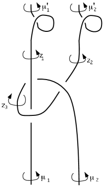
Figure 2:

We will use the Wirtinger presentation of the fundamental group of the string link to compute cohomology, using the following lemma. This simple lemma forms the basis for the Fox calculus and its relationship to group cohomology. Any statement made in this article about the Fox calculus is derived from this lemma together with the definition of a 1-cocycle.

Lemma 4.1

Suppose that a presentation $<x_{i},i\in I|r_{j},j\in J>$ is given for the group $\pi$, and an action $\pi\to\mbox{Aut}(M)$ is given. Then

1. A 1-cocycle with values in $M$ is determined by its values on the $x_{i}$.

2. Given a collection of elements $m_{i}\in M,i\in I$, there exists a (unique) 1-cocycle $f$ on the free group generated by the $x_{i}$ satisfying $f(x_{i})=m_{i}$ (with respect to the composite action $<x_{i}>\to\pi\to\mbox{Aut}(M)$).

3. The cocycle $f$ given in the previous assertion well-defines a 1-cocycle on $\pi$ if and only if $f(r_{j})=0$ for all $j$.

     

Fix a $\pi$-module $M$ determined by an action $e:\pi\to\mbox{Aut}(M)$.

Denote by $K$ the free group on $\{\mu_{i},z_{i},\mu_{i}^{\prime}\}$. Let $f\in Z^{1}(K;M)$ be some 1-cocycle on $K$, which, according to Lemma 4.1, is uniquely determined by the values of $f$ on the free generators. Then using the fact that $f$ is a cocycle, i.e. a crossed homomorphism on the free group, one computes:

$$f(\alpha\beta\alpha^{-1}\gamma^{-1}) = f(\alpha)+e(\alpha)f(\beta)-e(\beta)f(\alpha)-f(\gamma)$$

$$= (1-e(\beta))f(\alpha)+e(\alpha)f(\beta)-f(\gamma)$$

Lemma 4.1 implies that $f$ determines a 1-cocycle on $\pi$ if and only if for each Wirtinger relation $\alpha\beta\alpha^{-1}\gamma^{-1}$ one has $f(\alpha\beta\alpha^{-1}\gamma^{-1})=0$.

We use the Fox calculus to reduce the computation of cocycles to linear algebra. Restrict to $M=F$ and $e=\epsilon$. Notice that in Equation 4 the elements $e(\alpha),e(\beta)$, and $e(\gamma)$ are in the set $\{t_{i}\}_{i=1}^{n}$. Thus each Wirtinger relation determines a row in a $c\times(n+c)$ matrix using Equation 4 in the following way:

1. The columns correspond to the (ordered) $(n+c)$-tuple

   $$(\mu_{1},\cdots,\mu_{n},z_{1},\cdots,z_{c-n},\mu_{1}^{\prime}\cdots\mu_{n}^{\prime}).$$

2. The rows correspond to the relations, so the row corresponding to the relation $\alpha\beta\alpha^{-1}\gamma^{-1}$ has $1-e(\beta)$ in the column corresponding to $\alpha$, $e(\alpha)$ in the column corresponding to $\beta$, and $-1$ in the column corresponding to $\gamma$.

For example, a crossing with Wirtinger relation $\mu_{i}z_{j}\mu_{i}^{-1}(\mu_{k}^{\prime})^{-1}$ contributes a row with $1-t_{j}$ in the $i$th column, $t_{i}$ in the $(n+j)$th column, and $-1$ in the $(c+k)$th column. Write this matrix $\pmatrix{A&B&C\cr}$ where $A$ is a $c\times n$ matrix, $B$ is $c\times(c-n)$, and $C$ is $c\times n$.

From Lemma 4.1 one immediately concludes the following.

Lemma 4.2

Given a collection $\lambda_{1},\cdots,\lambda_{n},$ $\tau_{1},\cdots,\tau_{c-n},\lambda_{1}^{\prime},\cdots\lambda_{n}^{\prime}\in F$, there is a cocycle $f\in Z^{1}(\pi;F)$ satisfying $f(\mu_{i})=\lambda_{i}$, $f(z_{i})=\tau_{i}$, and $f(\mu_{i}^{\prime})=\lambda_{i}^{\prime}$ if and only if

$$\pmatrix{A&B&C}\pmatrix{\lambda_{1}\cr\vdots\cr\lambda_{n}\cr\tau_{1}\cr\vdots\cr\tau_{c-n}\cr\lambda_{1}^{\prime}\cr\vdots\cr\lambda_{n}^{\prime}\cr}=0$$ (4)

or, equivalently

$$\pmatrix{A&B}\pmatrix{\lambda_{1}\cr\vdots\cr\lambda_{n}\cr\tau_{1}\cr\vdots\cr\tau_{c-n}\cr}=-C\pmatrix{\lambda_{1}^{\prime}\cr\vdots\cr\lambda_{n}^{\prime}\cr}$$ (5)

     

The matrix $\pmatrix{A&B&C\cr}$ will be important in what follows. We will call it the Wirtinger–Fox matrix of the string link. The next lemma substitutes for Proposition 2.3 in the present context.

Lemma 4.3

The square matrix $\pmatrix{A&B\cr}$ has entries in $\Lambda={\bf Z}[t_{1},t_{1}^{-1},\cdots,t_{n},t_{n}^{-1}]$. Its determinant is a Laurent polynomial in the $t_{i}$ whose value at $1$ equals $\pm 1$. Therefore $\pmatrix{A&B\cr}$ is invertible over $\Lambda_{S}$ and hence also over $F$.

Proof. From its definition $\pmatrix{A&B\cr}$ has entries in $\Lambda$. If we set all the $t_{i}$ equal to $1$, the equation

$$(1-\epsilon(\beta))f(\alpha)+\epsilon(\alpha)f(\beta)-f(\gamma)=0$$

reduces to

$$f(\gamma)=f(\beta)$$ (6)

at each crossing. This implies that if $a:\Lambda\to{\bf Z}$ denotes the augmentation $t_{i}\mapsto 1$, then the system of linear equations over ${\bf Z}$

$$a\pmatrix{A&B}\pmatrix{x_{1}\cr\vdots\cr x_{n}\cr y_{1}\cr\vdots\cr y_{c-n}\cr}=-a(C)\pmatrix{s_{1}\cr\vdots\cr s_{n}\cr}$$

has a unique integer solution for any choice of $s_{1},\cdots,s_{n}$. One way to see this explicitly is to number the crossings as follows: let the first crossing be the crossing at which the strand with Wirtinger generator $\mu_{1}$ ends, the second crossing is the crossing at which the strand with Wirtinger generator $\mu_{2}$ ends, and so forth, going through the $\mu_{i}$ and then the $z_{i}$ in order. With this choice of ordering of the generators, the matrix $a(A\ B)$ is upper triangular with 1s on the diagonal. Therefore the determinant of $a(A\ B)$ equals $1$. The lemma follows.          

To simplify and clarify notation, we define, for $Z=X,X_{1},X_{0},P$, or $p$

$$C^{i}(Z)=C^{i}(\pi_{1}(Z);F).$$

Since space and group cohomology agree for connected spaces in dimensions $0$ and $1$, $H^{i}(Z;F)$ is the cohomology of $C^{*}(Z)$ for these spaces for $i=0$ and $1$ (and even for all $i$ since each $Z$ is aspherical).

Also, define $C^{i}(X,P)=\mbox{Ker}\ C^{i}(X)\to C^{i}(P)$ and $C^{i}(X_{1},p)=\mbox{Ker}\ C^{i}(X_{1})\to C^{i}(p)$. We use similar notation for cocycles ($Z^{i}(Z)$) and coboundaries ($B^{i}(Z)$).

The inclusion $i_{1}:(X_{1},p)\to(X,P)$ induces maps on cochains. Since $\pi_{1}X_{1}$ is free on the $\mu_{i}^{\prime}$, Lemma 4.1 implies that $Z^{1}(X_{1})\cong F^{n}$ and that an identification is given by the assignment $f\mapsto(f(\mu_{1}^{\prime}),\cdots,f(\mu_{n}^{\prime}))$. On the other hand, Lemma 4.3 and Equation 5 show that the restriction map on 1-cocycles

$$i_{1}:Z^{1}(X)\to Z^{1}(X_{1})$$

taking $f$ to its restriction to $\pi_{1}(X_{1})$ is an isomorphism.

Note that $d^{0}:F=C^{0}(X)\to C^{1}(X)$ is given by $d^{0}(v)(x)=(1-\epsilon(x))v$. Since, for example, $1-\epsilon(\mu_{i}^{\prime})=1-t_{i}\neq 0$, $d^{0}$ is non-zero and hence injective. Similarly $d^{0}:F=C^{0}(X_{1})\to C^{1}(X_{1})$ is injective and so by naturality we conclude that

$$i_{1}:H^{1}(X;F)\to H^{1}(X_{1};F)$$

is an isomorphism of $F$-vector spaces of dimension $n-1$. A similar argument applies to show that $i_{0}:H^{1}(X;F)\to H^{1}(X_{0};F)$ is an isomorphism.

We claim that every map in the diagram

$$\begin{diagram}$$

is an isomorphism.

Indeed, since $C^{0}(X,P)=\mbox{Ker}\ C^{0}(X)\to C^{0}(p)=\mbox{Ker}\ Id:F\to F$, it follows that the natural projection $Z^{1}(X,P)\to H^{1}(X,P;F)$ is an isomorphism. Similarly $Z^{1}(X_{1},p)\to H^{1}(X_{1},p;F)$ is an isomorphism. Since $P$ is an arc, $\pi_{1}(P)=(1)$, so $C^{i}(P)\cong F$ for all $i$. The restriction map $C^{1}(X)\to C^{1}(P)$ takes a 1-cochain to its value at $1\in\pi_{1}X$. Since all 1-cocycles vanish on the identity element, $Z^{1}(X)\subset C^{1}(X,P)$. But since $Z^{1}(X,P)=Z^{1}(X)\cap C^{1}(X,P)$ we conclude that $F^{n}=Z^{1}(X)=Z^{1}(X,P)=H^{1}(X,P;F)$. A similar argument applies to $(X_{1},p)$. Finally the five lemma shows that the left vertical map in the diagram is an isomorphism, and so all maps in the diagram are isomorphisms.

This shows how to interpret $\gamma(L)$ as a matrix. Just define $\gamma(L)$ to be the matrix representing the composition of isomorphisms

$$\begin{diagram}$$

The isomorphism $\alpha_{0}$ takes a cocycle $f$ to the vector $(f(\mu_{1})\cdots,f(\mu_{n}))$ and the isomorphism $\alpha_{1}$ takes a cocycle $f$ to the vector $(f(\mu_{1}^{\prime})\cdots,f(\mu_{n}^{\prime}))$.

The following observation will be important in a later section. Using Equation 5 and the definition of $\gamma(L)$, for each $i=1,\cdots,n$ there is a (unique) vector $(z_{1i},\cdots,z_{c-n\ i})$ so that

$$\pmatrix{A&B\cr}\pmatrix{\gamma(L)_{1i}\cr\vdots\cr\gamma(L)_{ni}\cr z_{1i}\cr\vdots\cr z_{c-n\ i}\cr}=-C\pmatrix{0\cr\vdots\cr 1\cr\vdots\cr 0\cr}.$$

This implies the following.

Proposition 4.4

The Wirtinger–Fox matrix $(A\ B\ C)$ of a projection of a string link $L$ and the Gassner matrix $\gamma(L)$ are related by the formula

$$\pmatrix{A&B\cr}\pmatrix{\gamma(L)\cr Z\cr}=-C$$ (7)

where $Z$ is some matrix that depends on the projection.          

To see that $\gamma(L)$ gives the classical Gassner representation when restricted to pure braids, one can either check by hand that this construction gives the correct value on the standard generators of the pure braid group, or else one can observe that the standard definition in terms of free group automorphisms gives rise via cohomology (or equivalently the Fox calculus) to the same $\gamma(L)$. We leave the details to the reader.

5 Concordance and boundary links

In this section we prove that $\gamma(L)$ is an I-equivalence invariant of $L$ and vanishes on boundary links. Let ${\cal C}_{n}$ denote the group of I-equivalence classes of pure $n$-component string links.

Theorem 5.1

The assignment to a string link $L$ the matrix $\gamma(L)$ defines an I-equivalence invariant of $L$. Moreover the induced function on the group of I-equivalence classes of pure $n$-component string links

$${\gamma}:{\cal C}_{n}\to GL_{n}(F)$$

is a group homomorphism.

Proof. Suppose that $L$ and $L^{\prime}$ are I-equivalent string links. Let $X$ and $X^{\prime}$ denote the complements of $L$ and $L^{\prime}$ in $D^{2}\times I$, and let $Y$ denote the complement of an embedding of $n$ copies of $I\times I$ in $D^{2}\times I\times I$ exhibiting the concordance. Thus, using the obvious notation, we have a commutative diagram of inclusions:

$$\begin{diagram}$$

Applying cohomology with twisted coefficients in $F={\bf Q}(t_{1},\cdots,t_{n})$ to this diagram and invoking Proposition 2.3 we see that in the following commutative diagram all maps are isomorphisms.

$$\begin{diagram}$$

Every cohomology group in the top and bottom rows are canonically identified with $F^{n}$ as described in the previous section. With these identifications the two top horizontal and bottom two horizontal isomorphisms are given by the identity map. Since $\gamma(L)$ is given by the composite of the two isomorphisms along the left edge and $\gamma(L^{\prime})$ is given by the composite of the two isomorphisms along the right edge it follows that $\gamma(L)=\gamma(L^{\prime})$. The fact that $\gamma$ is a group homomorphism when restricted to pure string links was observed in Section 2.          

We next show that $\gamma(L)$ is trivial on boundary string links. When combined with Theorem 5.1 this implies that the Gassner invariant is trivial on string links that are I-equivalent to boundary links.

The most convenient definition of boundary link in the context of string links is the following.

Definition 5.2

Let $G(x_{1},\cdots,x_{n})$ denote the free group on the generators $x_{i}$. A string link $L$ with $n$ components and complement $X=D^{2}\times I-L$ is called a boundary string link provided there exists a homomorphism

$$\phi:\pi_{1}X\to G(x_{1},\cdots x_{n})$$

so that

$$\phi(\mu_{i})=x_{i}=\phi(\mu_{i}^{\prime})$$

for each $i=1,\cdots n$ (with the $\mu_{i}$ as above).

The standard transversality argument shows that this is equivalent to the existence of $n$ disjointly embedded surfaces $E_{1},\cdots,E_{n}$ in $D^{2}\times I$ so that the boundary of each $E_{i}$ is a circle decomposed into two arcs, one of which is the $i$th component of the string link and the other which made up of three pieces in $\partial(D^{2}\times I)$ in the form $A\times\{0\}\cup\{b\}\times I\cup A\times\{1\}$ where $A\subset D^{2}$ is an arc from $p_{i}$ to $b\in\partial D^{2}$.

Theorem 5.3

If $L$ is a boundary string link, then $\gamma(L)$ is the identity transformation.

Proof. Write $G(x_{1},\cdots,x_{n})=\pi_{1}(\vee_{i=1}^{n}S^{1})$. There exists a homotopy commutative diagram

$$\begin{diagram}$$

where $\Phi$ induces $\phi$, and so that $j_{0}(x_{i})=\mu_{i}$ and $j_{1}(x_{i})=\mu_{i}^{\prime}$.

By definition, the Gassner invariant is the composite

$$(j_{0}^{*})^{-1}\circ(i_{0}^{*})^{-1}\circ i_{1}^{*}\circ j_{1}^{*}$$ (8)

where the $*$ superscripts refer to cohomology rel $p$ or $P$ with $F$ coefficients. But since the diagram commutes up to homotopy, and $\Phi_{|X_{i}}$ and $j_{i}$ are homotopy inverses for $i=0$ and $1$, the composite of Equation 8 is equal to the identity, as desired.          

The same analysis applies to the Burau representation. We leave the formulation to the reader.

At this point we note an observation of Le Dimet and X.-S. Lin that the braid group injects into the string link concordance group. A sketch of the argument follows. Suppose a braid is concordant to the trivial braid. The fundamental group of the complement of the braid includes in the group of the complement of the concordance. By Stallings’ Theorem [20] the inclusion induces isomorphisms on the lower central series of these groups. Hence, the automorphism induced by the braid is trivial on the lower central series of the free group since it coincides with the automorphism induced by the trivial braid. Since the free group is residually nilpotent, this automorphism is trivial and hence the braid is trivial since the automorphism determines the braid.

6 String link closure and a factorization of the Alexander polynomial

In this section we use the results of Section 4 to derive a factorization of the Alexander polynomial of the closure of a string link in terms of the Gassner matrix and a certain relative Reidemeister torsion invariant. We also give a general method to relate the Alexander polynomial of the link closure and the knot closure of a string link. (This is closely related to the factorization found by Levine in [14].) The results of this section are consequences of two basic facts. The first is that the Alexander matrix of the closure of a string link factors over $F$ as a product of two matrices one of which is constructed from the Gassner matrix of the string link. The second fact is that the Gassner matrix has the same linear algebraic properties as the Alexander matrix of a (closed) link, but is a well defined concordance invariant.

In the case of a (pure) braid, we recover the well known fact that the Alexander polynomial of the closure of a braid is equal to $\det(I-\gamma(L)(11))/(1-t_{1})$. (Here $M(1,1)$ represents the $(1,1)$ minor of the square matrix $M$.) Another special (and well-known) case occurs for a $1$-component string link when our factorization says that the Alexander polynomial of the closure (a knot) is equal to a certain Reidemeister torsion associated to the string link. The factorization of the Alexander matrix of the closure also sheds light on what concordance information is carried by the higher Alexander ideals of the closure.

In the following, given an $n$-component string link $L$ let $\hat{L}$ denote the closure of $L$. Thus $\hat{L}$ is the link of $n$ circles in ${\bf R}^{3}$ obtained by adding $n$ “parallel” strands in ${\bf R}^{3}-D^{2}\times I$, the $i$th strand having endpoints $p_{i}\times\{0\}$ and $p_{i}\times\{1\}$, as indicated in Figure 3.

Figure 3:

We recall briefly the definition of the multi-variable Alexander polynomial of a link. Given an $n$-component link ($n\geq 2$) $\hat{L}$ in $S^{3}$ and a numbering of its components, let $\pi=\pi_{1}(S^{3}-\hat{L})$ be the fundamental group of the link complement, and let $\epsilon:\pi\to{\bf Z}^{n}=<t_{1}^{\pm 1},\cdots,t_{n}^{\pm 1}>$ be the abelianization map, taking a meridian to the component colored $i$ to $t_{i}$. A presentation of $\pi$ determines, via the Fox calculus, a matrix with ${\bf Z}[{\bf Z}^{n}]$ entries called the Alexander matrix for the presentation. The ideal in ${\bf Z}[{\bf Z}^{n}]$ generated by the $(n-1)\times(n-1)$ minors of this matrix turns out to be of the form $\Delta_{\hat{L}}\cdot J$, where $\Delta_{\hat{L}}\in{\bf Z}[{\bf Z}^{n}]$ and $J=\ker a:{\bf Z}[{\bf Z}^{n}]\to{\bf Z}$ is the augmentation ideal. The element $\Delta_{\hat{L}}$ is well defined up to units in ${\bf Z}[{\bf Z}^{n}]$, i.e. up to elements of the form $\pm t_{1}^{a_{1}}\cdots t_{n}^{a_{n}}$ (see [7, 8] and the paragraphs following the statement of Theorem 6.2 below). It is called the Alexander polynomial of the link $\hat{L}$.

Lemma 6.1

Let $\pmatrix{A&B&C\cr}$ denote the Wirtinger–Fox matrix of a (projection of a) string link $L$, as defined in Equation 4. Then

$$V_{\hat{L}}=\pmatrix{A+C&B\cr}$$

is the Alexander matrix of the closure $\hat{L}$ with respect to the Wirtinger presentation of the corresponding projection of the closure.

Proof. This follows from the fact that the Wirtinger presentation for the complement of $\hat{L}$ is obtained by setting $\mu_{i}=\mu_{i}^{\prime}$ in the Wirtinger presentation of the string link $L$.         

Theorem 6.2

The Alexander matrix for the closure $\hat{L}$ factors as

$$V_{\hat{L}}=\pmatrix{A&B\cr}\pmatrix{I_{n}-\gamma(L)&0\cr-Z&I_{c-n}\cr}$$

where $I_{n}$ and $I_{c-n}$ are identity matrices, and $Z$ is some $(c-n)\times n$ matrix with $F$ coefficients depending on the projection.

Proof. We have

$$V_{\hat{L}} = \pmatrix{A&B\cr}+\pmatrix{C&0\cr}$$

$$= \pmatrix{A&B\cr}(I+\pmatrix{A&B\cr}^{-1}\pmatrix{C&0\cr}\ )$$

$$= \pmatrix{A&B\cr}(I-\pmatrix{\gamma(L)&0\cr Z&0\cr})$$

The last equality uses Proposition 4.4.         

We now examine more closely how to derive the Alexander polynomial of a link from the Wirtinger presentation associated to a projection of the link. What we will see is that the Gassner matrix of a string link shares many important properties of the Alexander matrix for the Wirtinger presentation of a (closed) link.

The Wirtinger presentation associates to a projection of (a closed link) ${\hat{L}}$ a presentation of $\pi_{1}(S^{3}-\hat{L})$ such that each generator $x_{i}$ is a meridian to the link, and each crossing in the projection defines a relation of the form $x_{i}x_{j}x_{i}^{-1}x_{k}^{-1}$. This gives a presentation with $c$ generators and $c$ relations, where $c$ denotes the number of crossings in the projection. A geometric argument shows that any one of the relations is a consequence of the other $c-1$. Letting $V$ denote the Alexander matrix for this presentation, a simple computation using the Fox calculus shows that this implies there exists a vector

$$u=(u_{1},\cdots,u_{c})\in{\bf Z}[{\bf Z}^{n}]^{c}$$

each of whose entries $u_{i}$ is a unit in ${\bf Z}[{\bf Z}^{n}]$ so that

$$uV=0.$$

On the other hand, the interpretation of the Fox matrix as a differential in the group cohomology chain complex shows that if $a(x_{i})=t_{\alpha(i)}$ then

$$Vw=0,$$

where

$$w=\pmatrix{1-t_{\alpha(1)}\cr\vdots\cr 1-t_{\alpha(c)}\cr}.$$

We will use this to show that $\Delta_{\hat{L}}$ is equal to ${{\det(V(i,j))}\over{1-t_{\alpha(j)}}}$, were $M(i,j)$ denotes the matrix obtained from a matrix $M$ by removing its $i$th row and $j$th column.

The following lemma can be proven using linear algebra. We will prove it (up to signs) in Section 10 as an easy application of Reidemeister torsion.

Lemma 6.3

Let $M$ be an $n\times n$ matrix over a domain, and let $u=(u_{1},\cdots,u_{n})$ and $w=(w_{1},\cdots,w_{n})^{T}$ be a row and column vector so that

$$uM=0\mbox{ \ and \ }Mw=0.$$

Then the element in the fraction field

$$(-1)^{i+j}{{\det(M(i,j))}\over{u_{i}w_{j}}}$$

is independent of $i$ and $j$, i.e. if $u_{i},u_{p},w_{j},w_{q}$ are all non-zero, then

$$(-1)^{i+j}{{\det(M(i,j))}\over{u_{i}w_{j}}}=(-1)^{p+q}{{\det(M(p,q))}\over{u_{p}w_{q}}}.$$

     

From the discussion preceding Lemma 6.3 we see that if $V$ denotes the Alexander matrix of the link $\hat{L}$, then

$$\Delta_{\hat{L}}(t_{1},\cdots,t_{n})={{\det(V(i,j))}\over{1-t_{\alpha(j)}}}.$$

It turns out that the Gassner matrix $\gamma(L)$ of a string link has the same property as the Alexander matrix of a (closed) link obtained using the Wirtinger presentation, as the following proposition shows.

Proposition 6.4

Let $L$ be a string link and $\gamma(L)$ its Gassner matrix.

1. $$(I-\gamma(L))\pmatrix{1-t_{1}\cr\vdots\cr 1-t_{n}\cr}=0.$$

2. $$(t_{1}^{-1},(t_{1}t_{2})^{-1},\cdots,(t_{1}t_{2}\cdots t_{n})^{-1})(I-\gamma(L))=0.$$

Proposition 6.4 allows us to make the following definition.

Definition 6.5

Let $L$ be a string link of 2 or more components, with Gassner matrix $\gamma(L)$. The Alexander rational function of $L$ is the rational function

$$\Delta_{L}(t_{1},\cdots,t_{n})=(-1)^{i+j}(t_{1}\cdots t_{i}){{\ \det(I-\gamma(i,j))}\over{1-t_{j}}}.$$

Lemma 6.3 implies that $\Delta_{L}\in F$ is well defined and independent of $i$ and $j$. Of course, it is an $I$-equivalence invariant of the string link since $\gamma(L)$ is.

The following lemma is a useful step in proving Proposition 6.4.

Lemma 6.6

The Gassner matrix for the braid obtained by applying one full positive twist to the trivial braid is

$$(t_{1}\cdots t_{n})(\mbox{Id}+\pmatrix{1-t_{1}\cr\vdots\cr 1-t_{n}\cr}(t_{1}^{-1},\ (t_{1}t_{2})^{-1},\ \cdots,\ (t_{1}t_{2}\cdots t_{n})^{-1})).$$

Sketch of Proof. This is an easy computation using the Fox calculus and the fact that the automorphism of the free group which corresponds to this braid is given by conjugation by the element $(t_{1}\cdots t_{n})^{-1}$. We leave the details to the reader.         

Proof of Proposition 6.4.

1. Let $X$ denote the complement of $L$. To prove the first statement, it suffices to show that there is a 1-cocycle on $\pi_{1}(X)$ which takes the values $1-t_{i}$ on both $\mu_{i}$ and $\mu_{i}^{\prime}$. But there is an obvious one—the coboundary of the constant 0-cochain. Indeed, if $f=1\in F\cong C^{0}(\pi_{1}(X);F)$, then $(\delta f)\in C^{1}(\pi_{1}(X);F)$ is defined by $(\delta f)(x)=1-\epsilon(x)$. Thus $(\delta f)(\mu_{i})=1-t_{i}=(\delta f)(\mu_{i}^{\prime})$.

2. Notice that conjugating a string link by the braid which is obtained by applying one full positive twist to the trivial braid yields an isotopic string link. Using Lemma 6.6 this means that

   $$(t_{1}\cdots t_{n})(\mbox{Id}+wu)\gamma(L)=\gamma(L)(t_{1}\cdots t_{n})(\mbox{Id}+wu)$$ (9)

   where

   $$w=\pmatrix{1-t_{1}\cr\vdots\cr 1-t_{n}\cr}$$

   and

   $$u=(t_{1}^{-1},(t_{1}t_{2})^{-1},\cdots,(t_{1}t_{2}\cdots t_{n})^{-1}).$$

   Simplifying Equation 9 and using the fact proven in part 1 that $\gamma(L)w=w$ one obtains

   $$wu\ \gamma(L)=wu.$$

   Equating the first row of each side of this equation gives

   $$(1-t_{1})u\gamma(L)=(1-t_{1})u.$$

   Since $1-t_{1}$ is non-zero, the desired result follows.          

In the case of the 1-variable Alexander polynomial (and/or 1-colored string links) and the Burau representation, a slight modification of the definition is necessary. Let $\alpha:{\bf Z}[{\bf Z}^{n}]\to{\bf Z}[{\bf Z}]$ be the ring map taking each $t_{i}$ to $t$. Let ${\hat{L}}$ be a closed link and $V_{\hat{L}}$ an Alexander matrix for ${\hat{L}}$. First, it is not true in general that det$(\alpha(V_{\hat{L}})(11)/(1-t)$ is a polynomial. Instead, one defines the 1-variable Alexander polynomial of a link $\hat{L}$ to be

$$\bar{\Delta}_{\hat{L}}(t)=\det(\alpha(V_{\hat{L}})(11)).$$

That this is an invariant follows just as before from Lemma 6.3 along with the fact that $\alpha(V_{\hat{L}})$ has eigenvectors $\alpha(u)$ on the left and $(1,\cdots,1)^{T}$ on the right (because $(1-t,\cdots,1-t)^{T}$ is an eigenvector). Thus in this situation one defines the 1-variable Alexander polynomials by

$$\bar{\Delta}_{\hat{L}}(t)=\det(\alpha(V_{\hat{L}})(11))$$

and so it is sensible for us to define the 1-variable Alexander function for a string link $L$ to be

$$\bar{\Delta}_{L}(t)=t\det(I-\beta(L)(11)).$$

In these definitions it is unnecessary for the components to be colored or for the string link to be pure.

From the definitions we have (up to multiples of $t$)

$$\bar{\Delta}_{\hat{L}}=(1-t)\alpha(\Delta_{\hat{L}})$$

for closed links and

$$\bar{\Delta}_{L}=(1-t)\alpha(\Delta_{L})$$

for pure (or colored) string links.

A “coordinate free” definition of the Alexander function for string links can be given in terms of the reduced Gassner invariant and the reduced Burau invariant.

Lemma 6.7

1. Let $L$ be a pure string link and $\tilde{\gamma}(L):H^{1}(X_{0};F)\to H^{1}(X_{0};F)$ the reduced Gassner invariant. Then

   $$\Delta_{L}=\pm{{\ \det(I-\tilde{\gamma}(L))}\over{(t_{1}t_{2}\cdots t_{n})^{-1}-1}}.$$

2. Let $L$ be an arbitrary string link and $\tilde{\beta}(L):H^{1}(X_{0};{\bf Q}(t))\to H^{1}(X_{0};{\bf Q}(t))$ its reduced Burau invariant. Then

   $$\bar{\Delta}_{L}={{\det(I-\tilde{\beta}(L))}\over{t^{-1}+t^{-2}+\cdots+t^{-n}}}.$$

We will prove this lemma in Section 10.

We next use the factorization of Theorem 6.2 to obtain a factorization of the Alexander polynomial of the closure of the link in terms of the Alexander rational function of the string link.

In order to give a topological interpretation of this factorization, we introduce the torsion of a string link. We use Reidemeister torsion to avoid some algebraic complications arising from the fact that the ring $\Lambda$ is not a P.I.D., but also because torsion has many nice properties. (See Section 10 for an in depth discussion, including the definition of Reidemeister torsion. The basic reference for torsion and its properties is [17].)

Let $L$ be a string link; as before denote its exterior by $X$ and the two punctured discs in the boundary of $X$ by $X_{0}$ and $X_{1}$. Lemma 2.1 implies that $H^{*}(X,X_{1};F)=0$, so that the chain complex

$$C^{*}(X,X_{1};F)=\mbox{Hom}_{\Lambda}(C_{*}(\tilde{X},\tilde{X_{1}}),F)$$

is acyclic. Here $\tilde{X}$ refers to the ${\bf Z}^{n}$ cover of $X$. This chain complex is based by taking lifts of a (relative) cell structure on the pair $(X,X_{1})$.

Definition 6.8

Define $\tau(L)$, the Reidemeister torsion of a string link $L$, to be the Reidemeister torsion of the based, acyclic cochain complex $C^{*}(X,X_{1};F)$.

Thus $\tau(L)\in F^{*}$ and is well defined up to multiplication by units in $\Lambda$, i.e. up to multiplication by elements of the form $\pm t_{1}^{a_{1}}\cdots t_{n}^{a_{n}}$. It is a smooth invariant of the string link $L$. In particular, it is independent of the choice of cell structure. Moreover, standard properties of the torsion show that $\tau(L)$ is multiplicative with respect to multiplying string links, i.e. $\tau(L_{1}L_{2})=\tau(L_{1})\tau(L_{2})$. This also follows by simple linear algebra from the fact proven below that $\tau(L)=\det(A\ B)$, where $(A\ B\ C)$ denotes the Wirtinger–Fox matrix.

In the 1-variable case one makes the analogous definition. We denote by $\bar{\tau}$ the 1-variable torsion of a string link.

Notice that if $L$ is a braid then $\tau(L)=1$ since $X$ collapses to $X_{1}$.

In the following theorem the formulas are understood to hold only modulo units in ${\bf Z}[{\bf Z}^{n}]$.

Theorem 6.9

Let $L$ be a pure string link and let $\hat{L}$ denote its closure. Then the (multi-variable) Alexander polynomial of $\hat{L}$ is the product of the torsion of the string link $\tau(L)$ and the Alexander rational function of the string link $\Delta_{L}$:

$$\Delta_{\hat{L}}=\tau(L)\cdot\Delta_{L}.$$

Moreover, given a projection of the string link $L$, $\tau(L)=\det(A\ B)$ where $(A\ B\ C)$ is the Wirtinger–Fox matrix. In particular, $\tau(L)\in{\bf Z}[{\bf Z}^{n}]$ and $\tau(L)$ augments to $\pm 1$.

Similarly, for a (not necessarily pure) string link $L$ the single variable Alexander polynomial of $\hat{L}$ factors as

$$\bar{\Delta}_{\hat{L}}(t)=\bar{\tau}(L)\cdot\bar{\Delta}_{L}(t).$$

Proof. Lemma 4.3 says that the matrix $(A\ B)$ has entries in ${\bf Z}[t_{1}^{\pm 1},\cdots,t_{n}^{\pm 1}]$ and has determinant augmenting to $\pm 1$.

We first explain why $\tau(L)=\det(A\ B)$. It is easy to see (and well known) that the Wirtinger presentation comes from a cell structure. In the present context, the exterior $X$ of the string link $L$ has a cell structure with one $0$-cell, $2n+c$ $1$-cells labeled $\mu_{1},\cdots,\mu_{n},z_{1},\cdots,z_{n},\mu_{1}^{\prime},\cdots,\mu_{n}^{\prime}$, $c$ $2$-cells labeled by the crossings in the projection, and no higher dimensional cells. The cell structure for the subcomplex $X_{1}$ has the same $0$-cell, $1$-cells $\mu_{1}^{\prime},\cdots,\mu_{n}^{\prime}$, and no higher dimensional cells.

From this one concludes that the short exact sequence of based cochain complexes for the pair $(X,X_{1})$,

$$0\to C^{*}(X,X_{1};F)\to C^{*}(X;F)\to C^{*}(X_{1};F)\to 0$$

is

$$\begin{diagram}$$

By definition, $\tau(L)$ is the determinant of the differential $\delta^{1}_{(X,X_{1})}$. By construction, the matrix $(A\ B\ C)$ represents the differential $\delta^{1}_{X}$. Since the relative complex consists of cochains vanishing on the $\mu_{i}^{\prime}$, it follows that $\delta^{1}_{(X,X_{1})}$ is represented by the matrix $(A\ B)$, as claimed.

For convenience change the projection by isotoping $L$ to add a little “kink” on the first component near its initial point (and relabel the $z_{i}$) to obtain a new Wirtinger relation $\mu_{1}z_{1}^{-1}$. Then no other relation involves $\mu_{1}$. Taking this to be the first Wirtinger relation what is achieved is:

1. The first row of $(A\ B)$ has $1$ in the first entry, $-1$ in the $n+1$st entry, and zeros elsewhere.

2. The first column of $(A\ B)$ has $1$ in the first entry and zeros elsewhere.

This procedure does not change the determinant of $(A\ B)$ up to sign.

Recall that

$$\Delta_{\hat{L}}={1\over{1-t_{1}}}\det(V_{\hat{L}}(1,1)).$$

Using elementary row operations of the form

1. Add a multiple (by an element of $F$) of the $i$th row to the $j$th row for $2\leq i,j\leq c$

2. Interchange the $i$th row with the $j$th row for $2\leq i,j,\leq c$

the matrix $(A\ B)$ can be transformed into a matrix of the form

$$\pmatrix{1&0\cdots 0\ -1\ 0\cdots 0\cr\matrix{0\cr\vdots\cr 0\cr}&D\cr}$$ (10)

where $D$ is a diagonal matrix. Note that $\det(D)=\pm\det(A\ B)$.

The elementary row operations used only operate on the second through $c$th rows, and hence there exists a $c\times c$ matrix $E$ with determinant $\pm 1$ of the form

$$E=\pmatrix{1&0\cr 0&X\cr}$$

with $X$ a $(c-1)\times(c-1)$ matrix so that the matrix of Equation 10 is equal to $E\cdot(A\ B)$.

Thus

$$(1-t_{1})\Delta_{\hat{L}} = \det(V_{\hat{L}}(11))$$

$$= \det(X\cdot(V_{\hat{L}}(11)))$$

$$= \det((E\cdot V_{\hat{L}})(11))$$

$$= \det((E(A\ B)\pmatrix{I-\gamma(L)&0\cr-Z&I\cr})(11))$$

The last equality follows from Equation 6.2.

A little matrix arithmetic using the fact that the matrix of Equation 10 is equal to $E\cdot(A\ B)$ shows that

$$(E(A\ B)\pmatrix{I-\gamma(L)&0\cr-Z&I\cr})(11)=\pmatrix{D_{1}(I-\gamma(11))&0\cr Z^{\prime}&D_{2}\cr}$$

where $D=\pmatrix{D_{1}&0\cr 0&D_{2}\cr}$, $Z^{\prime}$ is some matrix, and $\gamma(L)(11)$ is the matrix obtained from $\gamma(L)$ by dropping the first row and column. Thus

$$(1-t_{1})\Delta_{\hat{L}} = \det\pmatrix{D_{1}(I-\gamma(11))&0\cr Z^{\prime}&D_{2}\cr}$$

$$= \det(D)\det(I-\gamma(11))$$

$$= \det(A\ B)\det(I-\gamma(11)).$$

Since det$(A\ B)=\tau(L)$, and $\det(I-\gamma(11))/(1-t_{1})=\Delta_{L}$, the theorem is proved in the multi-variable case. A similar argument works in the 1-variable case.          

Theorem 6.2 can also be used to get information about the higher Alexander ideals of the closure of a string link $L$. Recall that the $k$th Elementary Alexander ideal of a link, $E_{k}$, is the ideal in ${\bf Z}[{\bf Z}^{n}]$ generated by $c-k$ minors of an Alexander matrix $V$ for the link, where $c$ is the number of generators of the presentation defining $V$. For example, $E_{0}=0$ since the Alexander matrix is singular, and we saw above that $E_{1}$ is the product of the augmentation ideal with the Alexander polynomial $\Delta$.

Similar definitions apply to the 1-variable Alexander ideals.

As an immediate consequence of Theorem 6.2 we get the following.

Corollary 6.10

For $k\leq n$ the first $k$ Alexander ideals $E_{k}(\hat{L})$ of the closure $\hat{L}$ of a pure string link $L$ link vanish if and only if the Gassner matrix $\gamma(L)$ has the eigenvalue $1$ with multiplicity $k$. Similarly, the first $k$ one-variable Alexander polynomials of the closure $\hat{L}$ of a string link $L$ link vanish if and only if the Burau matrix $\beta(L)$ has the eigenvalue $1$ with multiplicity $k$.

In particular, a pure string link is in the kernel of the Gassner representation if and only if the first $n$ Alexander ideals of its closure vanish. Similar remarks apply to the Burau representation.

     

We finish this section by deriving a formula relating the (1-variable) Alexander polynomials of the link and knot closures of a string link, giving an alternative and more general approach to the formulas of [14].

As pointed out in [14] any such formula permits one to compare the Alexander polynomials of a closed link to the Alexander polynomial of a knot obtained by banding the components together; the choice of bands essentially gives a representation of the link as the closure of a string link.

Let $L$ be a pure $n$-component string link and let $B$ be any $n$-braid. The case of most interest is when $B$ is the braid in Figure 4, since the closure $\widehat{LB}$ is a reasonable definition for the “knot closure” of $L$. Clearly $\widehat{LB}$ is obtained from $\hat{L}$ by banding the components together.

Figure 4:

Recall that $\tilde{\beta}$ denotes the reduced Burau representation, $\bar{\Delta}_{\hat{L}}$ denotes the 1-variable Alexander polynomial of the closed link $\hat{L}$.

Theorem 6.11

With notation as above, The 1-variable Alexander polynomials of the link closure $\hat{L}$ and the knot closure $\widehat{LB}$ of a string link are related by the formula

$$\bar{\Delta}_{\hat{L}}=\bar{\Delta}_{\widehat{LB}}\cdot{{\det(I-\tilde{\beta}(L))}\over{{\det(I-\tilde{\beta}(L)\tilde{\beta}(B))}}}.$$

The correction term $\det(I-\tilde{\beta}(L))/\det(I-\tilde{\beta}(L)\tilde{\beta}(B))$ is a string link I-equivalence invariant of $L$.

(We use the reduced Burau representation for convenience. Alternatively one can use $\det(I-\beta(11))$ in this formula.)

Proof. Theorem 6.9 (in the 1-variable case) says that $\bar{\Delta}_{\hat{L}}=\bar{\tau}_{L}\bar{\Delta}_{L}$, and similarly for $LB$. Since $B$ is a braid, $\bar{\tau}_{B}=1$ and so $\bar{\tau}_{LB}=\bar{\tau}_{L}\bar{\tau}_{B}=\bar{\tau}_{L}$. Moreover, ${{\det(I-\tilde{\beta}(L))}\over{(t^{-1}+\cdots+t^{-n})}}=\bar{\Delta}_{L}$ by Lemma 6.7.

Hence

$${{\bar{\Delta}_{\widehat{LB}}}\over{\bar{\Delta}_{\hat{L}}}}={{\bar{\Delta}_{{LB}}}\over{\bar{\Delta}_{L}}}={{\det(I-\tilde{\beta}(LB))}\over{\det(I-\tilde{\beta}(L))}}.$$

The last assertion follows from Theorem 5.1.          

7 Some examples

We will give a few examples to illustrate how to use the invariants and at the same time we introduce some geometric constructions on string links. We will omit most computations, but remark that they are easily carried out using a computer algebra package using Equation 7. Given a string link, its concordance inverse is the string link given by reflecting the given string link through the plane ${\bf R}^{2}\times{1\over 2}$ and reversing the orientation of the components.

A simple argument shows that any string link whose closure is the trivial link is string link concordant to the trivial link. Thus if $L$ is any string link whose closure is trivial, then $\gamma(L)$ is the identity matrix.

Now consider the pair of links $L_{1}$ and $L_{2}$ illustrated in Figure 5.

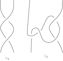
Figure 5:

Notice that $L_{1}$ and $L_{2}$ have the same closure, namely the Hopf link. The Gassner matrices for these links are:

$$\gamma(L_{1})=\pmatrix{t_{2}&1-t_{1}\cr(1-t_{2})t_{2}&1-t_{2}+t_{2}t_{1}\cr}$$

and

$$\gamma(L_{2})={1\over{-t_{1}-t_{2}+t_{2}t_{1}}}\pmatrix{1-2t_{2}-t_{1}+t_{1}t_{2}&t_{1}-1\cr(t_{2}-1)t_{2}&-t_{1}\cr}$$

so that $L_{1}$ and $L_{2}$ are not concordant as string links, even though their closures are isotopic.

For a linking number zero example, consider the links in Figure 6.

Figure 6:

The Gassner matrices are complicated but we can distinguish $\gamma(L_{3})$ from $\gamma(L_{4})$ using eigenvalues. As with all string links, both have $1$ as eigenvalue, the other eigenvalue for $\gamma(L_{3})$ (or equivalently $\tilde{\gamma}(L_{3})$) is

$${{t_{1}t_{2}(2-t_{1}-t_{2}+t_{1}t_{2})}\over{1-t_{1}-t_{2}+2t_{1}t_{2}}}$$

and the other eigenvalue for $\gamma(L_{4})$ is

$$-{{-2t_{2}t_{1}-t_{1}^{2}+t_{1}t_{2}^{2}+2t_{1}-t_{2}^{2}+t_{2}t_{1}^{2}+2t_{2}-1}\over{t_{1}^{2}-2t_{2}t_{1}^{2}-t_{2}-t_{1}+t_{2}^{2}+2t_{2}t_{1}-2t_{1}t_{2}^{2}+t_{2}^{2}t_{1}^{2}}}.$$

Thus these are not conjugate in the string link concordance group. (Notice that for 2-component string links the Gassner representation is abelian.)

These examples illustrate two interesting constructions which can be used to alter string links. The first adds a horizontal twist to one component, as illustrated in going from $L_{1}$ to $L_{2}$ in Figure 5 and in going from $L_{3}$ to $L_{4}$ in Figure 6. This yields different string links with the same closure. More generally one can add more twists and also add twists to different components, yielding hosts of examples of string links with the same closure but different Gassner matrices. We will show in the next section that in most cases this construction changes the Gassner matrix.

The second construction is a form of “Whitehead doubling” of one component, as illustrated in going from $L_{1}$ to $L_{3}$ and $L_{2}$ to $L_{4}$ in Figures 5 and 6. This is a subtle construction. Notice for example that if one Whitehead doubles each component, the result is a boundary string link and hence has trivial Gassner matrix.

As another example consider the two 3-component string links $L_{5}$ and $L_{6}$ in Figure 7. The first, $L_{5}$, is a braid. The second, $L_{6}$, is not.

Figure 7:

A computation shows that the $(1,1)$ entry of $\gamma(L_{6}L_{5}L_{6}^{-1})$ is not a Laurent polynomial in $t_{1},t_{2},t_{3}$. This implies that the conjugate $L_{6}L_{5}L_{6}^{-1}$ of the braid $L_{5}$ is not string link concordant to a braid. Since adding extra “trivial” components replaces the Gassner matrix by its direct sum with the identity matrix, we obtain the following theorem.

Theorem 7.1

For $n\geq 3$ The pure braid group on $n$ components is not normal in the pure string link concordance group.          

(Recall, by the comment at the end of Section 5, the braid group is a subgroup of the string link concordance group.)

Finally, we mention an example that shows that in the context of I-equivalence of string links, the Gassner invariant is not faithful. In [5] an example of a two component link $\hat{L}$ is given with the property that it is not concordant to a boundary link even though all its Milnor invariants are trivial. A string link, $L$, can be built from this link in such a way that a direct calculation shows the Gassner matrix is the identity. On the other hand, $L$ cannot be I-equivalent to a trivial link. If it were, then forming the connected sum of it closure $\hat{L}$ with knots $J_{1}$ and $J_{2}$ would yield a link $\hat{L^{\prime}}$ that is concordant to the trivial link. But then forming the connected sum of $\hat{L^{\prime}}$ with the mirror images of $J_{1}$ and $J_{2}$ would yield a link $\hat{L^{\prime\prime}}$ that is concordant to a split link formed as the union of the mirror images of $J_{1}$ and $J_{2}$. This is a boundary link but is also concordant to $\hat{L}$

8 Random walks and labelings of string links

In this section we begin by recalling a “probabilistic” interpretation of the Burau representation for string links studied in [15], and then extend it to give a similar interpretation of the Gassner representation. In that article the authors assign to a string link diagram with $n$ strands an $n\times n$ matrix with coefficients in the field ${\bf Q}(t)$ of rational functions in one indeterminate $t$. The $(i,j)-$th entry of this matrix is a sum (possibly infinite) over all the paths in the diagram of a string link starting at $p_{i}\times\{0\}$ and ending at $p_{j}\times\{1\}$ weighted in the following way. A path in the diagram is a “random walk” along the components (moving in the direction of the strands) of the string link such that whenever one comes to a crossing, one can either jump up or down, or one can continue without jumping. Notice there may be arbitrarily long paths; in the string link of Figure 2 there are paths which loop around as many times as one likes by jumping up at the right crossing, or going around the kinks.

The weight $w(p)\in{\bf Q}(t)$ of a path $p$ is defined to be the product over each crossing $c$ along $p$ of $w_{c}$

$$w(p)=\prod_{c}w_{c},$$

where

$$w_{c}=\cases{t^{\pm 1}&if the path $p$ goes under at the crossing c\cr 1-t^{\pm 1}&if the path $p$ jumps up at the crossing c\cr 1&if the path $p$ goes over at the crossing c\cr 0&if the path $p$ jumps down at the crossing c\cr}$$

The sign $\pm 1$ is chosen to be the sign of the crossing. Define a matrix by $\beta_{i,j}=\sum_{p}w(p)$ where the sum is over all paths $p$ that begin at $(p_{i},0)$ and end at $(p_{j},1)$. In [15], is shown that this sum converges to a rational function for any string link, and that the resulting matrix is invariant under Reidemeister moves. When restricted to braids this gives the Burau representation. We will outline simple proofs and generalize these facts to the Gassner representation below.

The relationship to the approach of the previous sections is as follows. Consider the following labeling scheme for string link diagrams. Think of a diagram of a string link as a graph in $R^{2}$ such that every vertex has valence 4 except for the endpoints. Define a labeling of the string link with value in a vector space $V$ to be an assignment of an element of $V$ to each edge in this graph.

We introduce a labeling that gives the Gassner representation. For this we must keep track of which strand one is on, i.e. we work with colored string links. The vector space $V$ is taken to be the field $F={\bf Q}(t_{1},\cdots,t_{n})$ of rational functions in $n$ variables. We will use $t_{o}$ (resp. $t_{u}$) to denote the variable with subscript the color of the over (resp. under) strand in the diagram.

Theorem 8.1

Fix a colored string link diagram.

1. Given any collection of $n$ elements $\lambda_{i}^{\prime}\in F,i=1,\cdots,n$, there exists a unique labeling of the diagram with values in $F$ such that

(a) The labeling at the $i$th top edge (the edge containing the point $p_{i}\times\{1\}$) is $\lambda_{i}^{\prime}$.

(b) At a positive crossing, if the four edges are labeled $S,E,W,N$ in such a way that the strands of the string link go as the diagram (Figure 8),

Figure 8:

then $S,E,W,N\in F$ satisfy the rules:

$$E = t_{o}W+(1-t_{u})N$$

$$S = N$$

and at a negative crossing, if the four edges are labeled $S,E,W,N$ in such a way that the strands of the string link go as the diagram (Figure 9),

Figure 9:

then $S,E,W,N$ satisfy the rules:

$$S = t_{o}^{-1}N+t_{o}^{-1}t_{u}(1-t^{-1}_{u})W$$

$$E = W.$$

2. Let $G(L)$ be the matrix whose $(i,j)$th entry is equal to the labeling of the $i$th bottom edge for the unique labeling satisfying the above equations with $\lambda_{k}^{\prime}=\delta_{jk}$. Then $G(L)=\gamma(L)$.

In terms of random walks, this says that if one assigns the local weight at a crossing by the rule:

$$w_{c}=\cases{t_{o}^{\pm 1}&if the path $p$ goes under at the crossing c\cr\sigma_{\pm}(1-t_{u}^{\pm 1})&if the path $p$ jumps up at the crossing c\cr 1&if the path $p$ goes over at the crossing c\cr 0&if the path $p$ jumps down at the crossing c\cr}$$

where the sign is the sign of the crossing and $\sigma_{+}=1,\sigma_{-}=t_{o}^{-1}t_{u}$, then the sum over all paths starting from the middle of the edge to the top $i$-th edge gives a labeling where the top $k$-th edge is labeled by $\delta_{ik}$.

Sketch of Proof of Theorem 8.1. The proof is virtually the same as that of Lemma 4.2. Notice that a labeling in the theorem has the property that the labels on the two edges which pass over a crossing are equal. Thus there is a one-to-one correspondence between such labelings of a string link diagram with values in $F$ and $Z^{1}(\pi,F)$. Moreover, if we set the $t_{i}$ equal to $1$ the equations reduce to $E=W$ and $N=S$ which has a unique solution given a labeling of the top strands.         

The labeling scheme is so flexible that we were led to wonder if there are other invariants satisfying such a simple linear system. Specifically, given any field, one can seek an assignment of local weights at a crossing so that the corresponding labeling obtained by summing over all paths as above is invariant under Reidemeister moves.

In general, suppose that some local weights are assigned as follows:

$$w_{c}=\cases{a_{o,u}^{\pm}&if the path $p$ goes under at the crossing c\cr b_{o,u}^{\pm}&if the path $p$ jumps up at the crossing c\cr c_{o,u}^{\pm}&if the path $p$ goes over at the crossing c\cr d_{o,u}^{\pm}&if the path $p$ jumps down at the crossing c\cr}$$

where $a_{o,u}^{\pm},b_{o,u}^{\pm},c_{o,u}^{\pm},d_{o,u}^{\pm}$ are arbitrary elements in some fixed field, and the $\pm$ is determined by the sign of the crossing c.

If there exists a string link invariant which assigns to a string link diagram a matrix whose $ij$-entry is the sum of the products of weights over all paths from the $i$th initial point to the $j$th endpoint of the string link, then the Reidemeister moves force some complicated algebraic relationships to hold between the elements $a_{o,u}^{\pm},b_{o,u}^{\pm},c_{o,u}^{\pm},d_{o,u}^{\pm}$ of the field. Even if one can find elements satisfying all these algebraic relationships, there may not exist a solution or it may not be unique if one exists. For these reasons we restricted our search to choices of weights for which the arguments of Section 4 for the Gassner representation extend. For simplicity we only considered choices of weights for which the resulting link invariants are “balanced” in the sense that changing the choice of coloring of the link gives an equivalent invariant. Thus we required the following two properties to hold.

1. (Homogeneity) if we re-index the components by a permutation, then the resulting matrix is obtained by permuting indices.

2. (Nondegeneracy) There is a ring map from the field to ${\bf C}$ so that the resulting linear system over ${\bf C}$ has a unique solution.

Under these conditions, a laborious calculation can be used to solve all relations imposed by invariance under Reidemeister moves. It turns out that there are essentially only two solutions. We omit the entirely calculational proof.

Theorem 8.2

Let $\nu$ be a string link invariant taking $n$-component pure string links to $n\times n$ matrices over some field, and suppose that $\nu$ is obtained by taking a string link to the matrix whose $ij$-entry is the sum of the products of weights over all paths from the $i$th initial point to the $j$th endpoint of the string link. If conditions $(C_{1})$ and $(C_{2})$ are satisfied, then $\nu$ is either a homomorphic image of the Gassner representation, or else is determined entirely by the pairwise linking numbers of the closure of the string link.          

We finish this section by giving an application of the random walk point of view for the Gassner invariant. The following theorem has a simple proof, although it is not at all obvious how to prove it starting with either the homological or the Fox calculus definitions of the Gassner invariant. This exhibits one advantage of the “random walk” approach to the Gassner representation, namely difficult linear algebra is simplified by the use of geometric series.

Given a string link $L$, let $T(L)$ be the string link obtained from $L$ by adding a (negative) horizontal twist to the first strand, as explained in the previous section and illustrated in Figure 10.

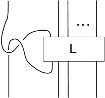
Figure 10:

The next result shows how to compute the Gassner matrix for $T(L)$ in terms of the Gassner matrix for $L$.

Theorem 8.3

Let $L$ be an $n$ component pure string link and $T(L)$ obtained from $L$ by adding a negative horizontal twist to the first strand as illustrated above. Suppose that

$$\gamma(L)=\pmatrix{a&{\bf b}\cr\bf{c}&D\cr}$$

where $a\in\Lambda_{S}$, ${\bf b}$ is an $n-1$ row vector, ${\bf c}$ is an $n-1$ column vector, and $D$ is an $(n-1)\times(n-1)$ matrix. Let

$$\alpha(a)={1\over{1-a(1-t_{1}^{-1})}}.$$

Then

$$\gamma(T(L))=\pmatrix{(1-t_{1}^{-1})+t_{1}^{-2}\alpha(a)a&t_{1}^{-1}\alpha(a){\bf b}\cr t_{1}^{-1}\alpha(a){\bf c}&D+(1-t_{1}^{-1})\alpha(a){\bf cb}\cr}.$$

Moreover, if $a\neq 1$, then the string links $L,T(L),T(T(L)),\cdots$ are all distinct in the string link concordance group but have isotopic closures.

In general, if $L$ is any pure string link with $\gamma(L)\neq I$, then adding horizontal twists to some component gives an infinite family of string links with the same closure as $L$ which are pairwise distinct in the pure string link concordance group.

Proof. Let $\gamma_{ij}$ denote the $i,j$ entry of $\gamma(L)$ and let $\gamma^{\prime}_{ij}$ denote the $i,j$ entry of $\gamma(T(L))$. Of course $a=\gamma_{11}$. Call the leftmost crossing in Figure 10 “crossing $1$”, the next crossing “crossing 2”; all other crossings of $T(L)$ are crossings of $L$ itself.

Consider first the entry $\gamma^{\prime}_{11}$. We can enumerate all random walks starting at the initial point of the first strand and ending at the endpoint of the first strand. We will ignore all walks that jump down at any crossing since these have weight zero and do not contribute to $\gamma^{\prime}$. Looking at Figure 10 above, we see that there is a path which jumps up at crossing 1; this path has total weight $1-t_{1}^{-1}$. Any other (non-zero weight) random walk passes under crossing 1, over crossing 2, and into the region corresponding to the string link $L$. If this random walk is to end up at the endpoint of the first strand of $T(L)$ it must emerge from the box at the endpoint of the first strand of $L$. This walk can then either

1. pass under at crossing 2 and then end, or

2. jump up at crossing 2 and enter the box labeled $L$ again.

Thus we can partition the set of all random walks contributing to $\gamma_{11}^{\prime}$ according to how many times they pass through the box labeled $L$. We already calculated that the (unique) walk never passing through this box contributes $1-t_{1}^{-1}$ to $\gamma_{11}^{\prime}$. A moment’s thought will convince the reader that the sum of weights over all random walks passing through the box once is $t_{1}^{-1}\gamma_{11}t_{1}^{-1}=t_{1}^{-2}\gamma_{11}$. Similarly the sum of weighs over all random walks passing through the box twice is $t_{1}^{-1}\gamma_{11}(1-t_{1}^{-1})\gamma_{11}t_{1}^{-1}=t_{1}^{-2}\gamma_{11}^{2}(1-t_{1}^{-1})$. In general the contribution to $\gamma_{11}^{\prime}$ of the random walks passing through the box $n$ times (for $n>0$) is $t_{1}^{-2}\gamma_{11}^{n}(1-t_{1}^{-1})^{n-1}$.

Summing over $n$ yields

$$\gamma_{11}^{\prime} = 1-t_{1}^{-1}+t_{1}^{-2}\gamma_{11}+\cdots+t_{1}^{-2}\gamma_{11}^{n}(1-t_{1}^{-1})^{n-1}+\cdots$$

$$= 1-t_{1}^{-1}+t_{1}^{-2}\gamma_{11}(1+\gamma_{11}(1-t_{1}^{-1})+\gamma_{11}^{2}(1-t_{1}^{-1})^{2}+\cdots)$$

$$= 1-t_{1}^{-1}+t_{1}^{-2}\gamma_{11}\ {1\over{1-\gamma_{11}(1-t_{1}^{-1})}}$$

$$= 1-t_{1}^{-1}+t_{1}^{-2}\gamma_{11}\alpha(a)$$

(The use of geometric series here is what makes the argument using random walks easy.)

The other three entries are computed in exactly the same way. For example, if $i$ and $j$ are bigger than $1$, then a random walk in $T(L)$ from the bottom $i$th endpoint to the top $j$th endpoint can either pass directly through $L$ to the $j$th endpoint of $L$, contributing $\gamma_{ij}$, or else it can go to the first endpoint of $L$ and jump up at crossing 2 and pass back into the box labeled $L$. This shows that the bottom right matrix in $\gamma(T(L))$ is the sum of $D$ and some expression involving $\gamma_{i1}$, $\gamma_{1,j}$, and $\gamma_{11}$. We leave the verification that the formula we give is correct to the reader.

Next consider the function

$$f:\Lambda_{S}\to\Lambda_{S}$$

given by the formula

$$f(a)=1-t^{-1}+{{t^{-2}a}\over{1-a(1-t^{-1})}}.$$

Let $z=1-t^{-1}$ and suppose that $a$ has power series expansion

$$a=a_{0}+\sum_{i=N}^{\infty}a_{i}z^{i}$$

where the $a_{i}\in{\bf Q}(t_{2},\cdots,t_{n})$ and $N>0$. Since we are assuming $a\neq 1$ we must consider two cases

1. $a_{0}\neq 1$ or

2. $a_{0}=1$ and $a_{N}\neq 0$.

A simple calculation shows that

$$f(a)-a={z\over{1-za}}(1-a)^{2}.$$ (11)

Thus in the first case when $a_{0}\neq 1$ the power series expansion for $f(a)$ is given by

$$f(a)=a_{0}+(a_{1}+(1-a_{0})^{2})z+o(z^{2})$$

and hence applying $f$ repeatedly one sees that the $(1,1)$-entry of the Gassner matrix for $T^{k}(L)$ is

$$a_{0}+(a_{1}+k(1-a_{0})^{2})z+o(z^{2})$$

so that in this case the string links $L,T(L),T(T(L)),\cdots$ are pairwise distinct in the string link concordance group.

The argument breaks down when $a_{0}=1$ and so we use a different argument in this case. Expanding $f(a)-a$ as a power series using Equation 11 we find that if $a_{0}=1$, the first nontrivial term in the expansion of $f(a)-a$ is $(a_{N})^{2}z^{2N+1}.$ Hence, the coefficient of $z^{2N+1}$ in the expansion of $f^{k}(a)=f\circ f\cdots\circ f(a)$ is $a_{2N+1}+k(a_{N})^{2}$. In particular these are distinct for distinct values of $k$ and the result is proved in this case.

The last assertion of the theorem follows from Theorem 3.4 since one can add a twist to any component, not just the first.

     

9 Dominance by finite type invariants

If we are allowed to replace some crossings of a string link with transverse double points, we get a singular string link. Applying the (now standard) method of extending link invariants to singular link invariants, the Gassner representation can be extended canonically to singular string links. In this section we will show that the coefficients in a Taylor expansion of the Gassner representation are finite type invariants.

Fix a string link with $n$ components and let $z_{i}=1-t_{i}$. For a multiple index $I=(i_{1}\cdots i_{j})$, with $i_{k}\in\{1,2,\cdots,n\}$, we denote $|I|=i_{1}+\cdots+i_{j}$, and $z^{I}=z_{i_{1}}\cdots z_{i_{j}}$. Taking the Taylor expansion of the matrix $\gamma(L)$ around $(t_{1},t_{2},\cdots,t_{n})=(1,1,\cdots,1)$, we obtain

$$\gamma(L)=\sum_{|I|=0}^{\infty}b_{I}(L)z^{I}.$$

The coefficients $b_{I}(L)$ are obviously invariants of string links. An invariant of string links is said to be finite type of order $\leq k$ if it vanishes on any singular string link with more than $k$ double points. See [3].

Theorem 9.1

The invariant $b_{I}(L)$ is of finite type of order $\leq|I|$.

Proof. Suppose we are given a string link diagram for a string link $L$ and suppose that $k$ crossings in this diagram are chosen. There are $2^{k}$ string links obtained by changing the signs of these crossings, labeled by a sequence of signs $\sigma\in(\pm)^{k}$. Call these various (embedded) string links $L_{\sigma}$.

For convenience, add a small kink near the endpoints of each strand. The proof will follow from a manipulation of an equation like Equation 7, but, since we wish to relate string links whose diagram differ at some crossings, it is most convenient to use presentations of the fundamental groups of the complements of the $L_{\sigma}$ with the same set of generators. Thus instead of the Wirtinger presentation we will use a larger set of generators for the fundamental group. Choose one generator for each edge in the 4-valent graph given by a (generic) projection of the string link. As before, label the bottom strands $\mu_{1},\cdots,\mu_{n}$ and the top strands $\mu_{1}^{\prime},\cdots,\mu_{n}^{\prime}$, and call the intermediate generators say $w_{i}$. An example of the labeling scheme is indicated in Figure 11.

Figure 11:

For each $\sigma\in(\pm)^{k}$, the fundamental group of the complement of $L_{\sigma}$ has a presentation similar to the Wirtinger presentation, but with extra relations obtained by setting two generators equal if they correspond to the same “overstrand”. Each crossing determines two relations. In the example of Figure 11, the first crossing along the first strand determines the relations $\mu_{1}w_{1}^{-1}$ and $w_{1}w_{5}\mu_{1}^{-1}w_{4}^{-1}$.

Applying the Fox calculus to the resulting presentation for $\pi_{1}(D^{2}\times I-L_{\sigma})$ with respect to the ordered basis $\{\mu_{1},\cdots,\mu_{n},w_{1},\cdots,w_{r},\mu_{1}^{\prime},\cdots,\mu_{n}^{\prime}\}$ one obtains as before a matrix

$$\pmatrix{A^{\prime}_{\sigma}&B_{\sigma}^{\prime}&C_{\sigma}^{\prime}\cr}$$

and the identical argument as the one given in Section 4 shows that for each $\sigma$ there exists a matrix $W_{\sigma}$ so that

$$\pmatrix{\gamma(L_{\sigma})\cr W_{\sigma}\cr}=-\pmatrix{A_{\sigma}^{\prime}&B_{\sigma}^{\prime}\cr}^{-1}C_{\sigma}.$$ (12)

For notational ease we rewrite

$$M_{\sigma}=\pmatrix{A_{\sigma}^{\prime}&B_{\sigma}^{\prime}\cr}$$

and

$$X_{\sigma}=\pmatrix{\gamma(L_{\sigma})\cr W_{\sigma}\cr}$$

so that Equation 12 can be rewritten as

$$M_{\sigma}X_{\sigma}=-C_{\sigma}^{\prime}$$ (13)

Lemma 9.2

In Equation 13,

1. The matrix $C_{\sigma}^{\prime}$ is independent of $\sigma\in(\pm)^{k}$.

2. The matrix obtained from $M_{\sigma}$ by mapping each $t_{i}$ to $1$ has all entries either $1,-1$ or $0$ and has determinant equal to $\pm 1$.

3. If $\sigma,\sigma^{\prime}\in(\pm)^{k}$ are two sequences of signs that differ only in the $j$th entry so that $\sigma_{j}=1$ and $\sigma^{\prime}_{j}=-1$, , then $M_{\sigma}-M_{\sigma^{\prime}}$ depends only on $j$ and moreover the Taylor expansion of $M_{\sigma}-M_{\sigma^{\prime}}$ at $t_{i}=1$ has zero constant term.

Proof. 1. This follows from the fact that we added kinks near the endpoints of each strand, so that the relations involving the $\mu_{i}^{\prime}$ are independent of $\sigma$.

2. This follows from the fact that the pair of relations determined by each crossing are of the type $ab^{-1}$ and $acb^{-1}d^{-1}$ and the same argument as Lemma 4.3.

3. The matrix $M_{\sigma}-M_{\sigma^{\prime}}$ has zeros for all entries except for a $2\times 4$ submatrix corresponding to the two relations and four generators involved in the $j$th crossing. A simple computation (easily derived from the formulas of Theorem 8.1) finishes the argument.          

We continue with the proof of Theorem 9.1. Let $|\sigma|$ denote the number of $+$ signs in $\sigma$. Use $o(z^{l})$ to denote any power series with only terms of order $z^{I}$ for $|I|\geq l$. To prove that $b_{I}(L)$ is of finite type of order $\leq k$, it suffices to show

$$\sum_{\sigma\in(\pm)^{k}}(-1)^{|\sigma|}X_{\sigma}=o(z^{k}).$$

From the first assertion of Lemma 9.2 we see that

$$\sum_{\sigma\in(\pm)^{k}}(-1)^{|\sigma|}M_{\sigma}X_{\sigma}=0.$$ (14)

We will now prove the theorem by induction.

For $k=1$,

$$0=M_{+}X_{+}-M_{-}X_{-} = (M_{+}-M_{-})X_{+}+M_{-}(X_{+}-X_{-})$$

$$= M_{-}(X_{+}-X_{-})+o(z)$$

Since $M_{-}=P+o(z)$ where $P$ is an invertible integer matrix, its inverse is of the form $Q+o(z)$ where $Q$ is the inverse matrix. Thus

$$X_{+}-X_{-}=o(z)$$

as desired.

For the general case, assume the theorem is true for fewer than $k$ crossings. Expanding Equation 14 according to the last sign, we have

$$\sum_{\sigma^{\prime}\in(\pm)^{k-1}}(-1)^{|\sigma^{\prime}|}(M_{\sigma^{\prime}+}X_{\sigma^{\prime}+}-M_{\sigma^{\prime}-}X_{\sigma^{\prime}-})=0.$$

This can be rewritten as

$$0=\sum_{\sigma^{\prime}\in(\pm)^{k-1}}(-1)^{|\sigma^{\prime}|}M_{\sigma^{\prime}-}(X_{\sigma^{\prime}+}-X_{\sigma^{\prime}-})+\sum_{\sigma^{\prime}\in(\pm)^{k-1}}(M_{\sigma^{\prime}+}-M_{\sigma^{\prime}-})(-1)^{|\sigma^{\prime}|}X_{\sigma^{\prime}+}.$$

Now notice that in the second summand, the term $(M_{\sigma^{\prime}+}-M_{\sigma^{\prime}-})$ is independent of $\sigma^{\prime}$ by the third assertion of Lemma 9.2. Thus the second summand is $o(z^{k}):$

$$\sum_{\sigma^{\prime}\in(\pm)^{k-1}}(M_{\sigma^{\prime}+}-M_{\sigma^{\prime}-})(-1)^{|\sigma^{\prime}|}X_{\sigma^{\prime}+} = (M_{\sigma^{\prime}+}-M_{\sigma^{\prime}-})\sum_{\sigma^{\prime}\in(\pm)^{k-1}}(-1)^{|\sigma^{\prime}|}X_{\sigma^{\prime}+}$$

$$= (M_{\sigma^{\prime}+}-M_{\sigma^{\prime}-})\cdot o(z^{k-1})\ {\mbox{by induction}}$$

$$= o(z^{k})\ {\mbox{by the third assertion of Lemma \ref{wemrn}.}}$$

Hence

$$o(z^{k})=\sum_{\sigma^{\prime}\in(\pm)^{k-1}}(-1)^{|\sigma^{\prime}|}M_{\sigma^{\prime}-}(X_{\sigma^{\prime}+}-X_{\sigma^{\prime}-})$$ (15)

We continue, inducting on the length of $\sigma$. The goal is to successively eliminate all occurrences of $M_{\sigma}$ except for the one sequence $\sigma=(-,-,-,\cdots,-)$.

The next step is, using Equation 15,

$$o(z^{k}) = \sum_{\sigma^{\prime\prime}\in(\pm)^{k-2}}(-1)^{|\sigma^{\prime\prime}|}M_{\sigma^{\prime\prime}+-}(X_{\sigma^{\prime\prime}++}-X_{\sigma^{\prime\prime}+-})+M_{\sigma^{\prime\prime}--}(X_{\sigma^{\prime\prime}-+}-X_{\sigma^{\prime\prime}--})$$

$$= \sum_{\sigma^{\prime\prime}\in(\pm)^{k-2}}(-1)^{|\sigma^{\prime\prime}|}M_{\sigma^{\prime\prime}--}(X_{\sigma^{\prime\prime}++}-X_{\sigma^{\prime\prime}+-}+X_{\sigma^{\prime\prime}-+}-X_{\sigma^{\prime\prime}--})$$

$$\quad+\sum_{\sigma^{\prime\prime}\in(\pm)^{k-2}}(-1)^{|\sigma^{\prime\prime}|}(M_{\sigma^{\prime\prime}+-}-M_{\sigma^{\prime\prime}--})(X_{\sigma^{\prime\prime}++}-X_{\sigma^{\prime\prime}+-})$$

Using the same argument as before, we see that the second summand in the last line is $o(z^{k})$, since $(M_{\sigma^{\prime\prime}+-}-M_{\sigma^{\prime\prime}--})=o(z)$ and is independent of $\sigma^{\prime\prime}$, and because

$$\sum_{\sigma^{\prime\prime}\in(\pm)^{k-2}}(-1)^{|\sigma^{\prime\prime}|}(X_{\sigma^{\prime\prime}++}-X_{\sigma^{\prime\prime}+-})=o(z^{k-1})$$

by induction (the penultimate sign is fixed).

Thus we obtain

$$o(z^{k})=\sum_{\sigma^{\prime\prime}\in(\pm)^{k-2}}(-1)^{|\sigma^{\prime\prime}|}M_{\sigma^{\prime\prime}--}(X_{\sigma^{\prime\prime}++}-X_{\sigma^{\prime\prime}+-}+X_{\sigma^{\prime\prime}-+}-X_{\sigma^{\prime\prime}--})$$

An induction argument leads to

$$o(z^{k})=\sum_{\sigma\in(\pm)^{k}}(-1)^{|\sigma|}M_{-\cdots-}X_{\sigma}.$$ (16)

The inverse of $M_{-\cdots-}$ has a Taylor expansion of the form $Q+o(z)$ for an integer matrix $Q$, and so inverting $M_{-\cdots-}$ in Equation 16 finishes the proof.         

10 Torsion and the Alexander function

In this section we re-examine the results of Section 6 using the more sophisticated methods of Reidemeister torsion. In particular, the factorization of the Alexander polynomial of a link will be seen as an easy consequence of a Mayer-Vietoris formula for Reidemeister torsion. Our purpose in including this material is multifold: for expository reasons, to sharpen the results of Theorem 6.9, to obtain a topological proof, to give a topological interpretation of the determinant of $(A,B)$, and to fit the Gassner representation for string links in the broader context of knot and link theory. We also us torsion to give simple and appealing proofs of Lemmas 6.3 and 6.7. It is also our belief that the methods of torsion are underused in knot theory and often provide a powerful framework to analyze knots and links. (Exceptions include Fox and Milnor’s use of the interpretation of the Alexander polynomial in terms of torsion to obstruct knot slicing [9] and [12] in which a similar interpretation of a twisted Alexander polynomial related to Casson-Gordon invariants is used to obstruct slicing algebraically slice knots. Another important reference is [22], in which Reidemeister torsion is applied to the study of links to vastly simplify much of the previous work on link polynomials as well as to extend the theory.)

For convenience we work with chain complexes and homology instead of cochain complexes and cohomology. As remarked in Theorem 3.1 the homology and cohomology Gassner representations are equivalent.

In its most common form, Reidemeister torsion is an invariant of a based, acyclic complex over a field. Milnor in [17] shows how to extend the definition to non-acyclic complexes, provided one chooses in addition a basis for the homology of the complex. From another point of view the Reidemeister torsion provides an acceptable substitute for the order of a torsion module. It is in this full generality that the various facets of Alexander type invariants of knots and links can be related.

We recall the definition of $\tau$. First, if $V$ is a vector space over $F$ and ${\bf b}$, ${\bf c}$ are bases of $V$, let $[{\bf c}|{\bf b}]$ denote the determinant of the transition matrix $M$ where $c_{i}=\sum_{j}M_{i,j}b_{j}$. Now suppose that $C_{*}$ is a free based chain complex over a field. Denote the basis for $C_{i}$ by ${\bf e}_{i}$. Suppose also that bases $[{\bf h}_{i}]$ of $H_{i}(C_{*})$ is chosen.

We arbitrarily choose bases ${\bf b}_{i}$ for the boundaries $B_{i}=\mbox{Image }\ \partial_{i+1}\subset C_{i}$. We also choose arbitrary lifts $\tilde{{\bf b}}_{i}\in C_{i+1}$ of the ${\bf b}_{i}$. Finally we choose representative cycles ${\bf h}_{i}$ of the classes $[{\bf h}_{i}]$.

With respect these choices the torsion is defined to be the product

$$\prod_{i}[{\bf b}_{i}{\bf h}_{i}\tilde{{\bf b}}_{i-1}|{\bf e}_{i}]^{(-1)^{i}}.$$

It is well defined in $F^{*}/(\pm 1)$ (for a ring $A$ let $A^{*}$ denote the group of units in $A$); in particular it is independent of the choice of the ${\bf b}_{i}$, their lifts $\tilde{{\bf b}}_{i}$, and the choice of cycles, ${\bf h}_{i}$, representing the homology bases $[{\bf h}_{i}]$. For a cochain complex, defines the torsion by turning a cochain complex into a (negatively graded) chain complex via the trick $C_{i}=C^{-i}$.

Next suppose that $R$ is a domain and let $F$ denote its quotient field. Let $C_{*}$ be a finitely generated free chain complex over $R$. Notice that $H_{i}(C_{*}\otimes_{R}F)=H_{i}(C_{*})\otimes_{R}F$ since $F$ is flat over $R$. To deal with the situation when $C_{*}$ is not acyclic, suppose that for each $i$ a finitely generated free $R$ submodule $K_{i}\subset H_{i}(C_{*})$ is given such that the inclusion $K_{i}\subset H_{i}(C_{*})$ induces an isomorphism $K_{i}\otimes F\to H_{i}(C_{*}\otimes F)$. There may be many choices for $K_{i}$ and different choices will lead to a different torsion in general.

Then choosing bases ${\bf e}_{i}$ of $C_{i}$ and ${\bf h}_{i}$ of $K_{i}$ determines bases (over $F$) of $C_{*}\otimes F$ and $H_{i}(C_{*}\otimes F)$. As explained above, these bases determine a Reidemeister torsion $\tau(C_{*}\otimes F;{\bf h}_{i})\in F^{*}$.

The easy but crucial observation is that the image of $\tau$ in $F^{*}/R^{*}$ is independent of the bases ${\bf e}_{i}$. It does depend on the choice of $K_{i}$, but not of the choice of bases $[{\bf h}_{i}]$ of $K_{i}$ since changing bases of $K_{i}$ (over $R$) gives a determinant in $R^{*}$. For convenience denote the image of $\tau(C_{*}\otimes F;{\bf h}_{i})$ by $\tau(C_{*};K)\in F^{*}/R^{*}$. If $C_{*}\otimes F$ is acyclic we abbreviate this to $\tau(C_{*})$. Moreover, if $C_{*}=C_{*}(S;R)$ for some space $S$ we will use $\tau(S;K)=\tau(C_{*};K)$.

As an example, suppose that $M$ is a torsion module over $R$, and suppose that $M$ admits a finitely generated free $R$ resolution $0\to C_{n}\to\cdots\to C_{0}\to M\to 0$. Then $C_{n}\otimes F$ is acyclic and we call $\tau(C_{*})$ the order of $M$, denoted by $|M|$. A standard argument shows that $|M|$ is well defined, i.e. independent of the choice of resolution. Notice that if $M$ is a PID then $M$ admits a free resolution $0\to C_{1}\smash{\mathop{\longrightarrow}\limits^{\partial_{1}}}C_{0}\to M\to 0$. By definition $|M|=\det(\partial_{1})$ (mod $R^{*}$), coinciding with the usual definition of the order of a torsion module. From this perspective the Reidemeister torsion provides an extension to ${\bf Z}[{\bf Z}^{n}]$ of the standard knot theory methods applied to the P.I.D. ${\bf Q}[{\bf Z}]$.

Suppose now that

$$0\to C_{*}\to D_{*}\to E_{*}\to 0$$

is a short exact sequence of free, finitely generated $R$-complexes. Assume free submodules $K_{i}^{C}\subset H_{i}(C_{*})$, $K_{i}^{D}\subset H_{i}(D_{*})$, and $K_{i}^{E}\subset H_{i}(E_{*})$ are specified inducing isomorphisms when tensoring with $F$, so that the torsions $\tau(C_{*};K^{C})$, $\tau(D_{*};K^{D})$, and $\tau(E_{*};K^{E})$ are defined. Choosing bases for the $K$ determines bases for the $F$ homology of the complexes, and hence the homology long exact sequence can be viewed as a based, acyclic $F$ complex ${\cal H}_{*}$.

$$\begin{diagram}$$

(The grading is defined by the convention ${\cal H}_{3i}=H_{i}(E_{*}),{\cal H}_{3i+1}=H_{i}(D_{*})$, and ${\cal H}_{3i+2}=H_{i}(C_{*})$.) We denote its torsion by $\tau({\cal H})$. It is well defined, independent of the choice of bases for the $K$. The same argument as in [17, Theorem 3.2] shows that

$${\tau(C_{*};K^{C})\tau(E_{*};K^{E})}\tau({\cal H})={\tau(D_{*};K^{D})}.$$ (17)

We will also use a slight extension of the preceding formula. If $0\to C_{*}\to D_{*}\to E_{*}\to 0$ is a short exact sequence of based chain complexes over a field, and homology bases are chosen, then the Formula 17 is still true (and holds in $F^{*}/\pm 1$) provided the bases are chosen compatibly. What this means is that if ${\bf c,\ d,\ e}$ are the given bases for $C_{*},\ D_{*},\ E_{*}$ respectively and ${\bf\tilde{e}}\subset D_{*}$ is a lift of ${\bf e}$ to $D_{*}$ then one requires that the determinant of the change of basis matrix from ${\bf d}$ to $\{{\bf c,\tilde{e}}\}$ should be $\pm 1$.

We will now apply these ideas to the situation of string links. First we prove Lemmas 6.3 and 6.7. These provide a gentle introduction to computing with torsion.

Proof of Lemma 6.3. Assume that $M$ has rank $n-1$ or else the lemma is trivial. Consider the following acyclic based complex:

$$0\to F\smash{\mathop{\longrightarrow}\limits^{W}}F^{n}\smash{\mathop{\longrightarrow}\limits^{M}}F^{n}\smash{\mathop{\longrightarrow}\limits^{q}}F\to 0$$ (18)

where $F$ denotes the fraction field, $W(f)=fw$, and $q(f_{1},\cdots f_{n})=\sum_{i}u_{i}f_{i}$. We base the complex by taking the standard basis ${\bf e}=\{e_{i}\}$ in the vector spaces $F^{n}$ and the unit $1$ as a basis for $F$.

To compute the torsion we need to choose bases for the boundaries and lifts thereof. Write the complex (18) as

$$0\to D_{3}\to D_{2}\to D_{1}\to D_{0}\to 0.$$ (19)

Then let ${\bf\tilde{b}_{2}}=1$ so ${\bf b}_{2}=w$. Letting ${\bf\tilde{b}_{1}}=\{e_{1},\cdots,\hat{e}_{j},\cdots,e_{n}\}$ one has that ${\bf b}_{1}=\{Me_{1},\cdots,\widehat{Me}_{j},\cdots,Me_{n}\}$. Let ${\bf\tilde{b}_{0}}=e_{i}$ so that ${\bf b}_{0}=u_{i}$. Then

$$\tau(D_{*}) = {{[u_{i}|1]\ [{\bf b}_{2}{\bf\tilde{b}}_{1}|{\bf e}]}\over{[{\bf b_{1}}{\bf\tilde{b}}_{0}}|{\bf e}][1|1]}$$

$$= {{u_{i}\cdot(-1)^{j+1}w_{j}}\over{(-1)^{i+n}\det(M(ij))\cdot 1}}.$$

Since the left side is well defined and independent of $i$ and $j$, so is the right side.         

Proof of Lemma 6.7. We will prove this using the formula 17. We assume that the determinant of $I-\tilde{\gamma}$ (resp. $I-\tilde{\beta}$) is non-zero since if not both sides of each formula in Lemma 6.7 are zero from the definitions.

We begin by setting up the notation. Let $F={\bf Q}(t_{1},\cdots,t_{n})$. From the definitions the Gassner and reduced Gassner representations are related by the diagram

$$\begin{diagram}$$

where the horizontal rows are exact, $H^{1}(X_{0},p)\cong F^{n}$, $H^{1}(X_{0})\cong F^{n-1}$. Fix the basis for $H^{1}(X_{0},p)$ as in Section 4 and call it $\{e_{0},\cdots,e_{n}\}$. and the map labeled $w$ takes $1\in F$ to the vector

$$w=\pmatrix{1-t_{1}\cr\vdots\cr 1-t_{n}\cr}.$$

Recall from Proposition 6.4 that the vector $u=(t_{1}^{-1},\cdots,(t_{1}t_{2}\cdots t_{n})^{-1})$ satisfies $u(I-\gamma)=0$ and that $(I-\gamma)w=0$. Let $q:H^{1}(X_{0},p)\to F$ denote the map $q(z_{1},\cdots,z_{n})=\sum_{i}u_{i}z_{i}$.

Denote the matrix for $I-\gamma:H^{1}(X_{0},p)\to H^{1}(X_{0},p)$ in the given basis by $M$. Clearly the image of $e_{2},\cdots,e_{n}$ in $H^{1}(X_{0})$ form a basis. Use this basis for $H^{1}(X_{0})$ and continue to call it $e_{2},\cdots,e_{n}$. Then we have three based acyclic chain complexes and an exact sequence relating them described in the following diagram.

$$\begin{diagram}$$ (20)

In Diagram 20 the horizontal rows are based, acyclic complexes. Also, $w_{1}=1-t_{1}$ is the first entry in the vector $w$.

For notational ease call the top complex $C_{*}$, the middle complex $D_{*}$, and the bottom complex $E_{*}$. The reader can easily check that:

1. the short exact sequence $0\to C_{*}\to D_{*}\to E_{*}\to 0$ has compatible bases, and

2. the torsion of $D_{*}$ is exactly the torsion computed in the proof of Lemma 6.3, so

   $$\tau(D_{*})={{u_{1}w_{1}}\over{\det(M(11))}}=\Delta_{L}^{-1}.$$

Since the complexes are compatibly based and acyclic, the formula 17 implies that

$$\tau(C_{*})\tau(E_{*})=\tau(D_{*}).$$ (21)

But trivial computations show that $\tau(E_{*})=\det(\widetilde{M})^{-1}=\det(I-\tilde{\gamma})^{-1}$ and

$$\tau(C_{*})=q(w)=\sum_{i}u_{i}w_{i}=\sum_{i}(t_{1}\cdots t_{i})^{-1}(1-t_{i})=(t_{1}\cdots t_{n})^{-1}-1.$$

Substituting into Equation 21 yields

$$((t_{1}\cdots t_{n})^{-1}-1)\det(I-\tilde{\gamma})^{-1}=\Delta_{L}^{-1}.$$

This establishes the first statement in the Lemma.

For the second statement, repeat the argument, but this time with

$$F={\bf Q}(t),\ M=I-\beta,\ \widetilde{M}=I-\tilde{\beta}.$$

Also set

$$w=\pmatrix{1\cr\vdots\cr 1\cr}\mbox{ and }u=(t^{-1},t^{-2},\cdots,t^{-n})$$

since we saw in Section 6 that these are the left and right $1$ eigenvectors for the Burau representation.

Then again $\tau(D_{*})=\bar{\Delta}_{L}^{-1}$ but this time $\tau(E_{*})=\det(\widetilde{M})^{-1}=\det(I-\tilde{\beta})^{-1}$ and

$$\tau(C_{*})=q(w)=\sum_{i}u_{i}w_{i}=t^{-1}+t^{-2}+\cdots+t^{-n}.$$

Thus Equation 21 reads

$$(t^{-1}+t^{-2}+\cdots+t^{-n})\det(I-\tilde{\beta})^{-1}=\bar{\Delta}_{L}^{-1}$$

establishing the second claim.          

For the rest of this section $R=\Lambda={\bf Z}[{\bf Z}^{n}]={\bf Z}[t_{i},t_{i}^{-1}]$ and $F={\bf Q}(t_{1},\cdots,t_{n})$ is its quotient field.

The following theorem is “folklore”; it is well known in the case of knots. An excellent exposition of Reidemeister torsion in knot theory can be found in [22]. There the connections between Alexander polynomials of links and Reidemeister torsion are fully developed.

Theorem 10.1

Let $\hat{L}\subset S^{3}$ be an $n$-component link; $n>1$. Let $C_{*}=C_{*}(S^{3}-\hat{L};\Lambda)$ be the free $\Lambda$ chain complex of cellular chains in the universal abelian (i.e. ${\bf Z}^{n}$) cover of $S^{3}-\hat{L}$.

Then $C_{*}\otimes F$ is acyclic if and only if the Alexander polynomial $\Delta_{\hat{L}}$ is non-zero, and in this case

$$\Delta_{\hat{L}}=\tau(S^{3}-\hat{L})^{-1}.$$

Notice that when $\Delta_{\hat{L}}$ is zero, $\tau(S^{3}-\hat{L};K)^{-1}$ is a (non-zero) generalization of the Alexander polynomial which depends in general on the choice of free submodule $K\subset H_{*}(Z;\Lambda)$.

Proof of Theorem 10.1. We sketch the argument. Let $Z$ denote $S^{3}-\hat{L}$. The Wirtinger presentation of $\pi_{1}(Z)$ gives a 2-complex cellular structure for $Z$ (up to homotopy) provided we drop one of the relations, say the one coming from the first crossing. Take the basis ${\bf e}_{i}$ of $C_{*}$ to be the cellular basis. But then the boundary map from $2$-chains to $1$-chains in this basis is exactly the Alexander matrix with its first row dropped, which we denote by $V^{\prime}$. The boundary map from $1$-chains to $0$-chains is given by the $(c\times 1)$ matrix taking each 1-cell to the appropriate $1-t_{i}$. Thus the chain complex $C_{*}=0\to C_{2}\to C_{1}\to C_{0}\to 0$ looks like

$$\begin{diagram}$$

Choosing free submodules $K_{i}\subset H_{i}(Z;\Lambda)$ defines a torsion $\tau(Z;K)\in F^{*}/\Lambda^{*}$.

Note that $H_{0}(Z;F)=F/\langle 1-t_{i}\rangle=0$. Also $H_{2}(Z;F)$ is the kernel of $\partial_{2}$, and we have identified it with the kernel of the Alexander matrix with its first row dropped. Recall that the Alexander polynomial $\Delta_{\hat{L}}$ is just $\det(V(ij))/(1-t_{\alpha(j)})$ (where the labeling of the generators is taken so that the $j$th generator lies on the $\alpha(j)$th component.) Thus, $\Delta_{\hat{L}}\neq 0$ if and only if $\det(V(ij))\neq 0$ for each $i,j$ which is true if and only $\partial_{2}$ is injective.

Assume by relabeling if necessary that the first generator is part of the first component for the string link, i.e. $\alpha(1)=1$. Take $\tilde{{\bf b}}_{0}$ to be the first element $e_{1,1}$ of the basis ${\bf e}_{1}$, so that ${\bf b}_{0}=(1-t_{1})e_{1,1}$. Also take $\tilde{{\bf b}}_{1}={\bf e_{2}}$, so that ${\bf b}_{1}=V^{\prime}{\bf e_{2}}$. Also

Computing directly with the definition one sees that if the Alexander polynomial is non-zero, then

$$\tau = {{[{\bf b}_{0}|{\bf e}_{0}]\ [{\bf\tilde{b}}_{1}|{\bf e}_{2}]}\over{[{\bf b}_{1}|{\bf e}_{1}]}}$$

$$= {{(1-t_{1})\cdot 1}\over{\det(V(11))}}$$

$$= \Delta_{\hat{L}}^{-1}$$

     

We next wish to give our generalization of Theorem 6.9 using torsion. We first recall and set up some notation.

Let $L\subset D^{2}\times I$ be an $n$-component string link; $n>1$. Let $X$ denote the complement $(D^{2}\times I)-L$. Let $X_{0}$ and $X_{1}$ denote the punctured disks $(D^{2}-\{p_{i}\})\times\{0\}$ and $(D^{2}-\{p_{i}\})\times\{1\}$. Let $W$ be the complement of the closure $\hat{L}$ viewed as a link in the solid torus, so

$$W=X\cup X_{0}\times I$$

and let $Z$ be the complement of $\hat{L}$ in $S^{3}$, so that

$$Z=W\cup Q$$

where $Q$ is a solid torus.

Each of the spaces $X_{0},X_{1},X,W,Z$, and $Q$ has a $\Lambda$ (and hence also $F$) coefficient system defined by the abelianization maps on fundamental groups.

Lemma 10.2

1. The inclusion $W\subset Z$ induces isomorphisms $H_{i}(W;F)\to H_{i}(Z;F)$. These groups are zero except possibly if $i=1$ and $2$. Moreover,

   $$\tau(Z,W)=(1-t_{1}\cdots t_{n}).$$ (22)

2. The projections $X_{0}\times I\to X_{0}$, $X_{0}\times I\to X_{1}$, and the inclusion $X_{0}\subset X$ induce isomorphisms on $F$-homology. The homology groups $H_{i}(X_{0};\Lambda)$ are zero except for $i=1$ and $H_{1}(X_{0};\Lambda)=\Lambda^{n-1}$.

Proof. The excision theorem implies that the homology groups $H_{i}(Z,W)$ are isomorphic to $H_{i}(Q,T)$, where $T=\partial Q$ is a torus. The two generators of $\pi_{1}T$ can be taken to be the curve $\mu$ bounding a disk in $Q$ and $\lambda=\partial X_{0}$. The representation $\pi_{1}T\to{\bf Z}^{n}$ takes $\mu$ to $1$ and $\lambda$ to $1-t_{1}\cdots t_{n}$. Notice that $Q$ deforms to $\lambda$. It follows readily that $H_{i}(T;F)$ and $H_{i}(Q;F)$ vanish for all $i$. Thus $H_{i}(Q,T;F)=H_{i}(Z,W;F)=0$ for all $i$ and $\tau(Z,W)=\tau(Q,T)$. At this point we leave to the reader the elementary computation

$$\tau(Z,W)=\tau(Q,T)=(1-t_{1}\cdots t_{n}).$$

We have calculated in Section 2 that

$$H_{i}(X_{0};\Lambda)=\cases{\Lambda^{n-1}&if $i$=1\cr 0&otherwise.\cr}$$

and that with $F$ coefficients the inclusion $H_{*}(X_{0};F)\to H_{*}(X;F)$ is an isomorphism. The second assertion follows easily.          

The following notation will hold for the rest of this section. Let $K_{i}\subset H_{i}(W;\Lambda),\ i=1,2$ be free submodules so that the inclusion induces isomorphisms $K_{i}\otimes F\to H_{i}(W;F)$. For convenience denote the image of $K_{i}$ in $H_{i}(Z;\Lambda)$ by $K_{i}$ also. (Recall that by Lemma 10.2 $K_{i}$ injects into $H_{i}(Z;\Lambda)$.) Let $J=H_{1}(X_{0}\times I;\Lambda)$. Also denote the (injective) image of $J$ in the $\Lambda$-homology groups of $X_{0},X_{1}$ and $X$ by $J$. Notice that $J$ is canonical, i.e. no choices are involved in making its definition. In contrast, there is no natural choice of $K_{i}$ in general.

Theorem 10.3

Let $\Phi$ denote Mayer-Vietoris diagram

$$\begin{diagram}$$

The Mayer-Vietoris homology sequence with $F$ coefficients for $\Phi$ reduces to the sequence

$$0\to H_{2}(W)\to H_{1}(X_{0})\oplus H_{1}(X_{1})\smash{\mathop{\longrightarrow}\limits^{\xi}}H_{1}(X)\oplus H_{1}(X_{0}\times I)\to H_{1}(W)\to 0$$ (23)

Denote its torsion (which is defined once one specifies the spaces $K_{i}$ and $J$ in the manner described above) by $\tau({\cal H}(\Phi);K)$.

Then the map $\xi$ in the sequence (23) is given by the matrix

$$\xi=\pmatrix{I&I\cr\tilde{\gamma}&I\cr}$$

where $\tilde{\gamma}$ denotes the reduced Gassner representation.

Furthermore,

$$\tau(Z;K)^{-1}={{\tau(L)\ \tau({\cal H}(\Phi);K)}\over{1-t_{1}\cdots t_{n}}}$$ (24)

Where $\tau(L)$ is the torsion of the string link (defined in Section 6).

Finally, if $\Delta_{L}\neq 0$ then $K=0$,

$${{\tau(H(\Phi);K)}/{1-t_{1}\cdots t_{n}}}=\Delta_{L},$$

$$\tau(Z;K)^{-1}=\Delta_{\hat{L}},$$

and Equation 24 reduces to Theorem 6.9.

Proof. Lemma 10.2 shows that all the other groups in the Mayer-Vietoris sequence for $\Phi$ vanish. From the definition of the reduced (homology) Gassner matrix the map labeled $\xi$ in the sequence 23 is given in this basis by the matrix

$$\xi=\pmatrix{I&I\cr\tilde{\gamma}&I\cr}.$$

Applying Equation 17 to the Mayer-Vietoris sequence and using the fact that the torsion of a direct sum is the product of torsions, one concludes that

$$\tau({\cal H}(\Phi);K)={{\tau(X_{0}\times I;J)\ \tau(X;J)}\over{\tau(X_{0};J)\ \tau(X_{1};J)\ \tau(W;K)}}.$$ (25)

Notice, however, that $X_{0}\times I$ deforms to $X_{0}$ and $X_{1}$, and by the way we chose the bases for $J$ it follows that $\tau(X_{0}\times I;J)=\tau(X_{0};J)=\tau(X_{1};J)$. Thus Equation 25 reduces to

$$\tau({\cal H}(\Phi);K)={{\tau(X;J)}\over{\tau(X_{1};J)\ \tau(W;K)}}.$$ (26)

Now consider the pair $(Z,W)$. The complex $C_{*}(Z,W;F)$ is acyclic and the choice of bases for $K_{i}\subset H_{i}(W;\Lambda)$ were used to define the bases for $H_{i}(W;F)$ and $H_{i}(Z;F)$, it follows that the torsion of the long exact sequence in homology for the pair $(Z,W)$ is equal to $1$; in fact the sequence reduces to isomorphisms which are the identity in the given bases. Thus Equation 17 implies that

$$1={{\tau(W;K)\ \tau(Z,W)}\over{\tau(Z;K)}}$$

and so

$$\tau(W;K)=\tau(Z;K)\tau(Z,W)^{-1}.$$ (27)

Finally consider the pair $(X,X_{1})$. A similar argument as the previous paragraph shows that

$$1={{\tau(X_{1};J)\ \tau(X,X_{1})}\over{\tau(X;J)}}.$$ (28)

Combining Equations 22, 26, 27, and 28 yields

$$\tau(Z;K)^{-1}={{\tau(X,X_{1})^{-1}\ \tau({\cal H}(\Phi);K)}\over{1-t_{1}\cdots t_{n}}}.$$ (29)

Moreover $\tau(X,X_{1})=\tau(L)^{-1}$

Since we defined $\tau(L)$ using the (dual) cochain complex. Substituting this into Equation 29 establishes Equation 24.

Now recall that $\Delta_{L}$ is non-zero if and only if $\det(I-\tilde{\gamma})$ is non-zero. Since

$$\det(I-\tilde{\gamma})=\det\pmatrix{I&I\cr\tilde{\gamma}&I\cr},$$

it follows that $\Delta_{L}$ is non-zero if and only if $H_{*}(Z;F)=H_{*}(W;F)=K=0$ and in this case the sequence 23 shows that

$$\tau({\cal H}(\Phi))=\det(I-\tilde{\gamma}).$$

Thus Equation 29 reduces in this case to

$$\tau(Z)^{-1}={{\tau(L)\ \det(I-\tilde{\gamma})}\over{1-t_{1}\cdots t_{n}}}$$ (30)

Lemma 6.7 shows that $\Delta_{L}={{\det(I-\tilde{\gamma})}\over{((t_{1}\cdots t_{n})^{-1}-1)}}$. Notice that

$$1-t_{1}\cdots t_{n}=(t_{1}\cdots t_{n})((t_{1}\cdots t_{n})^{-1}-1).$$

Theorem 10.1 implies that $\tau(Z)^{-1}=\Delta_{\hat{L}}$.

Substituting these into Equation 30 and working modulo units in $\Lambda$ one obtains, when $\Delta_{L}\neq 0$, the formula

$$\Delta_{\hat{L}}=\tau(L)\ \Delta_{L}.$$

This is just the formula of Theorem 6.9.

     

Department of Mathematics pkirk@indiana.edu

Indiana University livingst@indiana.edu

Bloomington, IN 47405 zhewang@indiana.edu

References

- [1] M. N. Abdulrahim, Complex specializations of the reduced Gassner representation of the pure braid group, Proc. Amer. Math. Soc. 125 (1997), no. 6, 1617–1624.
- [2] M.F. Atiyah, V.K. Patodi, and I.M. Singer Spectral asymmetry and Riemannian geometry. II, Math Proc. Camb. Phil. Soc. 78 (1975), 405–432.
- [3] D. Bar-Natan On the Vassiliev knot invariants, Topology 34 (1995), no. 2, 423–472.
- [4] J. Birman Braids, links, and mapping class groups, Annals of Mathematics Studies No. 82, Princeton University Press, Princeton, N.J., 1974.
- [5] T. Cochran and K. Orr, Not all links are concordant to boundary links, Ann. of Math. (2) 138 (1993), no. 3, 519–554.
- [6] T. Cochran, Non-trivial links and plats with trivial Gassner matrices, Math. Proc. Cambridge Philos. Soc. 119 (1996), no. 1, 43–53.
- [7] R. Fox Free differential calculus. II. The isomorphism problem of groups, Ann. of Math. (2) 59, (1954) 196–210.
- [8] R. Fox A quick trip through knot theory, 1962 Topology of 3-manifolds and related topics (Proc. The Univ. of Georgia Institute, 1961) 120–167 Prentice-Hall, Englewood Cliffs, N.J.
- [9] R. Fox and J. Milnor Singularities of -spheres in -space and cobordism of knots, Osaka J. Math. 3 (1966) 257–267.
- [10] N. Habegger and X. S. Lin The classification of links up to link-homotopy, J. Amer. Math. Soc. 3 (1990), no. 2, 389–419.
- [11] V. Jones, A polynomial invariant for knots via von Neumann algebras, Bull. Amer. Math. Soc. 12 (1985), no. 1, 103–111.
- [12] P. Kirk and C. Livingston Twisted Alexander invariants, Reidemeister torsion, and the Casson-Gordon invariants, to appear, Topology (1996).
- [13] J.-Y. Le Dimet Enlacements d’intervalles et representation de Gassner, Comment. Math. Helv. 67 (1992), no. 2, 30-6-315.
- [14] J. Levine A factorization of the Conway polynomial, preprint (1997).
- [15] X.S. Lin, F. Tian, and Z. Wang Burau representations and random walks on string links, Pacific J. of Math 182 (1998) 289–302.
- [16] Long, D. D. On the linear representation of braid groups, Trans. Amer. Math. Soc. 311 (1989), no. 2, 535–560.
- [17] J. Milnor Whitehead torsion, Bull. Amer. Math. Soc. 72 1966 358–426.
- [18] J. Moody The faithfulness question for the Burau representation, Proc. Amer. Math. Soc. 119 (1993), no. 2, 671–679.
- [19] R. Penne Multi-variable Burau matrices and labeled line configurations, J. Knot Theory Ramifications 4 (1995), no. 2, 235–262.
- [20] J. Stallings Homology and central series of groups, J. Algebra 2 (1965) 170–181.
- [21] C. Squier,The Burau representation is unitary, Proc. Amer. Math. Soc. 90 (1984), no. 2, 199–202.
- [22] V. Turaev , Reidemeister torsion in knot theory, Russian Math. Surveys 41:1 (1986), 119–182.