Structures and Diagrammatics of Four Dimensional Topological Lattice Field Theories

Abstract

Crane and Frenkel proposed a state sum invariant for triangulated 4-manifolds. They defined and used new algebraic structures called Hopf categories for their construction. Crane and Yetter studied Hopf categories and gave some examples using group cocycles that are associated to the Drinfeld double of a finite group.

In this paper we define a state sum invariant of triangulated $4$-manifolds using Crane-Yetter cocycles as Boltzmann weights. Our invariant generalizes the 3-dimensional invariants defined by Dijkgraaf and Witten and the invariants that are defined via Hopf algebras. We present diagrammatic methods for the study of such invariants that illustrate connections between Hopf categories and moves to triangulations.

1 Introduction

Witten’s formulation [45] of an intrinsic definition of the Jones polynomial [22] based on physical models lead to the more rigorous mathematical definitions via representations of quantum groups that were given by Reshetikhin, Turaev, and Viro [40], [43]. These quantum invariants are speculated to generalize to higher dimensions. Such putative invariants have their origins in a theory of quantum gravity [4] and higher categories [5]. In relation to the current work, the following progress has been made.

Quantum spin networks were generalized by Crane-Yetter [16] to give $4$-manifold invariants that were based on Ooguri’s proposal [36]. The invariants can be used to compute the signature as shown in [41, 14, 15]. Birmingham-Rakowski [8] generalized the Dijkgraaf-Witten [18] invariant of 3-manifolds, defined by group 3-cocycles, to triangulated 4-manifolds using pairs of cocycles. Crane and Frenkel [13] constructed Hopf categories to define 4-manifold invariants, and they gave examples using canonical bases of quantum groups. In [17] Crane and Yetter used cocycles to construct Hopf categories.

In this paper we provide direct relations between the cocycle conditions of [17] and Pachner moves of $4$-manifolds, thus constructing a generalization of the Dijkgraaf-Witten invariants to dimension 4. The relations are established diagrammatically, providing connections between Hopf categorical structures and triangulations via dual graphs and their movies.

The current paper is self-contained, but the reader might enjoy our introduction to the subject given in [10], where many of our ideas and motivations are introduced in a more leisurely fashion. For the diagrammatic foundation of the invariants in dimension 3 see [25], [26], and [24]. For the algebraic approach see [9]. Finally, there is a relation to higher dimensional knot theory as found in [11].

Let us continue our motivational remarks. In $3$ dimensions, planar diagrams played a key role in the definitions of both knot invariants and manifold invariants. Such diagrams are convenient since they help one grasp the categorical and algebraic structures needed for defining invariants. One of the difficulties in generalizing to dimension $4$ or higher is the lack of such visualizations and diagrammatic machinery. The purpose of this paper is to provide basic diagrammatic tools to study $4$-manifold triangulations, and to use such formulations to define invariants.

In particular, we formulate the Crane-Frenkel approach in terms of cocycles as initial data and prove the invariance under Pachner moves in a diagrammatic way. We introduce spin networks for the study of such invariants. We hope that the present work serves as a basic tool in exploring the possibilities in higher dimensions.

There is a close relationship bewteen certain physical models in statistical mechanics and quantum field theory and the formulation of “quantum” invariants of knots, links and three-manifolds. We hope that this relationship continues into dimension four. In particular, one can hope that a four dimensional toplogical field theory (such as we study here) would be related to the calculation of amplitudes in quantum gravity. The naive reason for this hope is quite simple: An amplitude for quantum gravity must sum over the possible metrics on the four-dimensional spacetime. Averaging over metrics should in priniciple produce basic numbers that are metric-independent. In other words a valid process of averaging over metrics should produce topological invariants of the underlying four-space. Of course on the physical side it will be neccessary to extricate the topological part from the complexities of the model. On the pure mathematical side it will be neccessary to see the relevance of the mathematics. Nevertheless this hope for an application to quantum gravity is one of the forces that drives our project.

The organization of the paper is as follows. In Section 2, we review state sum invariants for triangulated manifolds in dimensions $2$ and $3$. We emphasize diagrammatic relations between triangulations and algebraic structures. At the end of the section, we summarize the idea of categorification in relation to the construction of higher dimensional invariants. In Section 3 we present diagrams of Pachner moves in dimension $4$. We also introduce singular moves in dimension $4$, and prove that singular moves together with $3$-dimensional Pachner moves imply $4$-dimensional Pachner moves. These Lemmas will be used to prove the well-definedness of our invariants. In Section 4 we give generalization of spin networks to dimension $4$. Triangulations are represented by movies of graphs, and these graph movies will be used to give a direct relation between Hopf category structures and triangulations. Cocycle conditions defined by [17] will be reviewed in Section 5. Symmetry of cocycles are defined. In Section 6 the state sum invariants will be defined, and will be proved to be well-defined in Section 7. Our proofs are diagrammatic. They provide the basic machinery necessary to define other invariants defined via Hopf categories. The axioms of Hopf categories are related to moves on triangulations of 4-manifolds in a manner similar to the relationship between Hopf algebras and moves on 3-manifolds. Section 8 reviews the definition of Hopf category and make the connection with the rest of the paper.

2 Quantum 2- and 3- manifold invariants

In this section, we review topological lattice field theories in dimension $3$ and explain how they are generalized from those in dimension $2$. First we review dimension $2$ following [21, 12] where semi-simple algebras are used. An alternative approach is given by Lawrence in [33] in which the algebra is assumed to be Frobinius. Next the Turaev-Viro [43] theory is reviewed following [9] and [26]. Invariants of 3-manifolds derived from Hopf algebras are presented following [12]. Alternative approaches are found in Kuperburg [30] and Kauffman-Radford [27]. Some of the summary appeared in [10]. We summarize Wakui’s defintion [44] of the Dijkgraff-Witten invariants [18], but here we show invariance using the Pachner Theorem. This section closes with a conceptual scheme for generalizing to dimension 4.

2.1

Topological lattice field theories in dimension $2$. Let $A$ denote a finite dimensional associative algebra over the complex numbers ${\bf C}$. Let $\{\phi_{i}|i=1,\cdots,n\}$ denote an ordered basis for $A$, and for $x,y,z\in\{1,\ldots,n\}$, let $C_{xy}^{z}$ denote the structure constant of the algebra $A$. Thus the multiplication between basis elements is given by the formula:

$$\phi_{x}\cdot\phi_{y}=\sum_{z}C_{xy}^{z}\phi_{z}.$$

Apply the associativity law, $(ab)c=a(bc)$, to the basis elements as follows:

$$(\phi_{a}\phi_{b})\phi_{c} = (\sum_{j}C_{ab}^{j}\phi_{j})\phi_{c}=\sum_{j,d}C_{ab}^{j}C_{jc}^{d}\phi_{d}$$

$$\phi_{a}(\phi_{b}\phi_{c}) = \phi_{a}(\sum_{i}C_{bc}^{i}\phi_{i})=\sum_{i,d}C_{ai}^{d}C_{bc}^{i}\phi_{d}.$$

In this way, we obtain the equation

$$\sum_{j}C_{ab}^{j}C_{jc}^{d}=\sum_{i}C_{ai}^{d}C_{bc}^{i}$$

whose geometrical interpretation will be presented shortly.

For $x,y\in\{1,2,\ldots,n(=dimA)\}$, define

$$g_{xy}=\sum_{u,v}C^{v}_{ux}C^{u}_{vy}.$$

Then this is invertible precisely when the algebra $A$ is semi-simple [21], and the matrix inverse $g^{xy}$ of $g_{xy}$ defines a bilinear form on the algebra $A$. The geometric interpretation of this bilinear form and that of the associativity identity will allow us to define from a semi-simple associative algebra, an invariant of 2-dimensional manifolds.

We follow the definition given in [21]. Let $T$ be a triangulation of a closed 2-dimensional manifold $F$. Let ${\cal N}=\{1,2,\cdots,n\}$. This is called the set of spins. Let ${\cal ET}=\{(e,f)|e\subset f\}$ be the set of all the pairs of edges, $e$, and faces, $f$, such that $e$ is an edge of $f$. The set ${\cal ET}$ is a partial flag. A labeling is a map $L:{\cal ET}\rightarrow{\cal N}$. Thus a labeling is an assignment of spins to all the edges with respect to faces. Given a labeling, we assign weightings to faces and edges as follows: Suppose that we are given functions $C$ and $g$, $C:{\cal N}^{3}\rightarrow{\bf C}$, $C(x,y,z)=C_{xyz}$, and $g:{\cal N}^{2}\rightarrow{\bf C}$, $g(x,y)=g^{xy}$. If a face has three edges labeled with spins $x,y,z$, then assign the complex number $C_{xyz}$ to the face. It is assumed that the function $C$ posesses a cyclic symmetry; so $C_{xyz}$ $=C_{yzx}$ $=C_{zxy}$. If an edge is shared by two faces, and the edge with respect to these faces receives spins $x$ and $y$, then assign the complex number $g^{xy}$ to the edge. Then define a partition function $\Psi(T)$ by $\sum_{L}\prod C_{xyz}g^{uv}$ where the sum is taken over all the labelings and the product is taken over all the elements of ${\cal ET}$. Values of $C_{xyz}$ and $g^{uv}$ are given in terms of the structure constants for the algebra and the bilinear form $g_{uv}$ in the fourth paragraph forward. First, we discuss topological aspects that motivate their definition.

In order for the partition function to be topologically invariant, it cannot depend on the choice of triangulation. There are two steps in constructing such an invariant quantity. First, we work topologically. There is a set of local moves to triangulations that suffices to relate any two triangulations of a given manifold. These moves were discovered by Pachner [37] in the general case of $n$-manifolds, and they generalize a classical theorem of Alexander [2]. Therefore for the partition function to be independent of the choice of triangulation, it is sufficient to prove that the weighting assigned to triangles and edges satisfies equations that correspond to these local moves. The second step, therefore, is algebraic. We seek functions $C$ and $g$ that satisfy these equations. We will indicate that the structure constants of an associative algebra can be used for the function $C$ and that the bilinear form on $A$ can be used to define the function $g$, as the notation suggests.

Let us consider the topological aspects. The Pachner moves in dimension 2 are depicted in Figure 1. The move on the left of Figure 1 is called the $(2\rightleftharpoons 2)$-move; that on the right is called the $(1\rightleftharpoons 3)$-move. The names of the moves indicate the number of triangles that are involved.

Figure 1: 2D Pachner moves

Figure 2: Associativity and a 2-dimensional Pachner move

We now intepret associativity and the bilinear form in a semi-simple algebra over ${\bf C}$ in terms of the Pachner moves. Specifically, the $(2\rightleftharpoons 2)$-Pachner moves is related to the associativity law $(ab)c=a(bc)$. The relationship is depicted in Figure 2. The dual graphs, indicated in the Figure by dotted segments, are sometimes useful for visualizing the relations between triangulations and the algebraic structure. The diagram given in Figure 3 illustrates the geometrical interpretation of the bilinear form $g_{xy}=\sum_{u,v}C^{v}_{xu}C^{u}_{yv}.$ In the figure, two triangles share two edges in the left picture, representing the local weighting $\sum_{u,v}C^{v}_{xu}C^{u}_{yv}$, and the right represents a single edge corresponding to $g_{xy}$. Finally, this relationship together with the associativity identity can be used to show that the partition function is invariant under the $(1\rightleftharpoons 3)$-Pachner move. The essence of the proof is indicated in Figure 4.

Figure 3: The semi-simplicity axiom and degenerate triangulations

Figure 4: Semi-simplicity, associativity, and the (3,1)-move

Having illustrated the algebra axioms diagrammatically, we turn to show how the structure constants and the bilinear form of associative semi-simple algebras solve the equations corresponding to the Pachner moves. Given, structural constants $C^{z}_{xy}$ and a non-degenerate bilinear form $g^{uz}$ with inverse $g_{uz}$, define $C_{xyu}$ by the equation (using Einstein summation convention of summing over repeated indices),

$$C_{xyu}\equiv g_{uz}C_{xy}^{z}.$$

Then since

$$\sum_{j}C_{ab}^{j}C_{jc}^{d}=\sum_{i}C_{ai}^{d}C_{bc}^{i}$$

the partition function defined in this way is invariant under the $(2\rightleftharpoons 2)$-move. Furthermore, we have (again, under summation convention)

$$C^{a}_{de}C^{j}_{ab}C^{d}_{jc}=C^{a}_{de}C^{d}_{ai}C^{i}_{bc}=g_{ie}C^{i}_{bc}=C_{ebc},$$

and so the partition function is invariant under the $(1\rightleftharpoons 3)$-move. In this way, a semi-simple finite dimensional algebra defines an invariant of surfaces. On the other hand, given a partition function one can define a semi-simple algebra with these structure constants and that bilinear form. In [21], this is stated as Theorem 3:

The set of all TLFTs is in one-to-one correspondence with the set of finite dimensional semi-simple associative algebras.

Observe that the $(1\rightleftharpoons 3)$-move follows from the $(2\rightleftharpoons 2)$-move and a non-degeneracy condition. In the sequel, we will see similar phenonema in dimensions 3 and 4.

In general, the idea of defining a partition function to produce a manifold invariant is (1) to assign spins to simplices of a triangulation, and (2) to find weightings that satisfy equations corresponding to Pachner moves. This approach, of course, depends on finding such solutions to (often extremely overdetermined) equations. Such solutions come from certain algebraic structures. Thus one hopes to extract appropriate algebraic structures from the Pachner moves in each dimension. This is the motivating philosophy of quantum topology.

In the following sections we review such invariants in dimension $3$ in more detail to explain such relations between triangulations and algebras.

2.2

Pachner moves in dimension $3$. In this section we review the Pachner moves [37] of triangulations of manifolds in dimension $3$. The Pachner moves in $n$-dimensions form a set of moves on triangulations such that any two different triangulations of a manifold can be related by a sequence of moves from this set. Thus, two triangulations represent the same manifold if and only if one is obtained from the other by a finite sequence of such moves. In Figure 5 the 3-dimensional Pachner moves are depicted, these are called the $(2\rightleftharpoons 3)$-move and the $(1\rightleftharpoons 4)$-move.

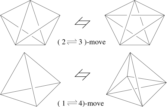
Figure 5: 3-dimensional Pachner moves

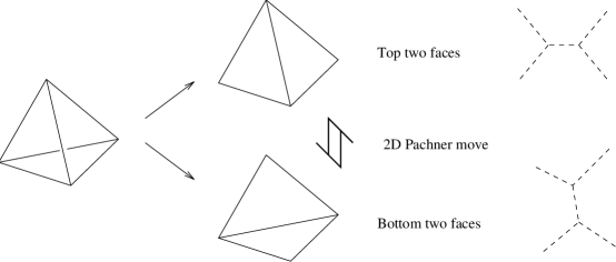
Figure 6: Movie of a tetrahedron and a 2-dimensional Pachner move

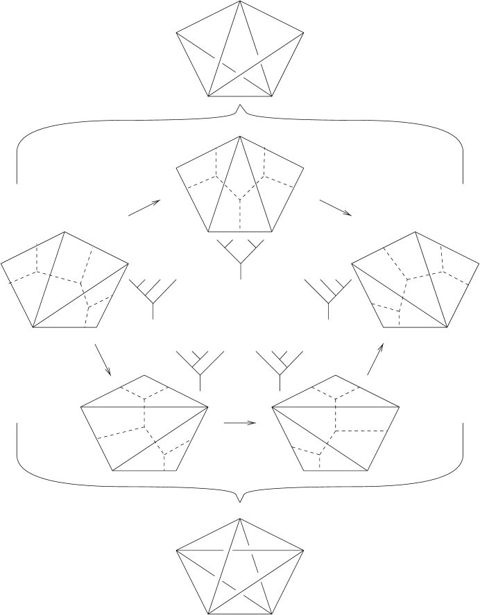
Figure 7: The pentagon, trees, and a 3-dimensional Pachner move

Notice that the 2-dimensional Pachner moves relate the faces of a tetrahedron. Specifically, the $(2\rightleftharpoons 2)$-move consists of two pairs of triangles and they together form a tetrahedron (Figure 6). Meanwhile, the $(1\rightleftharpoons 3)$-move relates three triangular faces of a tetrahedron to the remaining face. The three triangles form the central projection of a tetrahedron. Analogous facts are true for the 3-dimensional Pachner moves as well; let us explain. One side of each move is a union of $3$-faces of the boundary of a $4$-simplex and the other side of the move is the rest of the $3$-faces, and they together form the boundary of a $4$-simplex. For example, the $(1\rightleftharpoons 4)$-move indicates two 3-balls on the boundary of a 4-simplex as they appear in a central projection of the simplex.

In Figure 6, the relation between faces of a tetrahedron and their dual graphs is depicted. The middle picture shows pairs of front and back faces of a tetrahedron on the center left. Note that these pairs represent the $(2\rightleftharpoons 2)$ Pachner move (as indicated by the vertical double arrow in the middle). Thus the $(2\rightleftharpoons 2)$ Pachner move corresponds to a tetrahedron, a $1$-dimensionally higher simplex. On the right of the figure, the change on dual graphs is depicted by dotted lines. In Figure 7, a similar correspondence is depicted for the $(2\rightleftharpoons 3)$ Pachner move. Here faces of unions of tetrahedra are depicted from left to right, in two different ways that correspond to the Pachner move. These are the faces taken from the union of tetrahedra depicted in top and bottom of the figure, respectively. The dual graphs are also depicted, which are the graphs used for the Biedenharn-Elliott identity of the $6j$-symbols. This direct diagrammatic correspondence is pointed out in [9].

2.3

Turaev-Viro invariants. One way to view the Turaev-Viro invariants [43, 26] is to “categorify” the TLFT in dimension 2. In this process, the semi-simple algebra is replaced by a semi-simple monoidal category — namely the category of representations of $U_{q}(sl(2))$ where $q$ is a primitive $4r\/$th root of unity. First we review the definition of the Turaev-Viro invariants, and then explain the viewpoint mentioned above.

A triangulation of a $3$-manifold is given. A coloring, $f$, is admissible if whenever edges with colors $a,b,j$ bound a triangle, then the triple $(a,b,j)$ is a $q$-admissible triple in the sense that

1. $a+b+j$ is an integer,

2. $a+b-j$,  $b+j-a,$ and $a+j-b$ are all $\geq 0$

3. $a+b+j\leq r-2.$

If edges with labels $a,b,c,j,k,n$ are the edges of a tetrahedron such that each of $(a,n,k)$, $(b,c,n),$ $(a,b,j)$, and $(c,j,k)$ is a $q$-admissible triple, then the tetrahedron, $T$, receives a weight of $T_{f}=\mbox{$\left[\begin{array}[]{ccc}a&b&n\\ c&k&j\end{array}\right]_{q}$ }.$ If any of these is not admissible, then the weight associated to a tetrahedron is, by definition, 0.

For a fixed coloring $f$ of the edges of the triangulation of a 3- manifold $M$, the value

$$|M|_{f}=\Delta^{-t}\prod\Delta_{f(E)}\prod T_{f}$$

is associated where $t$ is the number of vertices in the triangulation, the first product is taken over all the edges in the triangulation, the second product is over all the tetrahedra, the factor $\Delta$ is a normalization factor (= const.) and $\Delta_{f(E)}$ is a certain quantum integer associated to the color of the edge $E$. To obtain an invariant of the manifold one forms the sum

$$|M|=\sum_{f}|M|_{f}$$

where the sum is taken over all colorings. Further details can be found in [43, 26] or [9].

Several points should be made here. First, the sum is finite because the set of possible colors is finite. Second, the quantity $|M|$ is a topological invariant because the $6j$-symbols satisfy the Beidenharn-Elliott identity and an orthogonality condition. The orthogonality is a sort of non-degeneracy condition on the $6j$-symbol. In [26, 9] it is shown how to use orthogonality and Beidenharn-Elliott (together with an identity among certain quantum integers) to show invariance under the $(1\rightleftharpoons 4)$ move. Third, the $6j$-symbol is a measure of non-associativity as we now explain.

The situation at hand can be seen as a categorification. In $2$-dimensions associativity $(ab)c=a(bc)$ played a key role. In $3$-dimensions the $6j$-symbols are defined by comparing two different bracketting $(V^{a}\otimes V^{b})\otimes V^{c}$ and $V^{a}\otimes(V^{b}\otimes V^{c})$ of representations $V^{a}$, $V^{b}$, and $V^{c}$. Here the algebra elements became vector spaces as we went up dimensions by one, and the symbol measuring the difference in associativity satisfies the next order associativity, corresponding to the Pachner move.

Given representations $V^{a}$, $V^{b}$, $V^{c}$, we can form their triple tensor product and look in this product for a copy of the representation $V^{k}$. If there is such a copy, it can be obtained by regarding $V^{k}$ as a submodule of $V^{a}\otimes V^{n}$ where $V^{n}$ is a submodule of $V^{b}\otimes V^{c}$, or it can be obtained as a submodule of $V^{j}\otimes V^{c}$ where $V^{j}$ is a submodule of $V^{a}\otimes V^{b}$. From these two considerations we obtain two bases for the set of $U_{q}(sl(2))$ maps $V^{k}\rightarrow V^{a}\otimes V^{b}\otimes V^{c}$. The $6j$-symbol is the change of basis matrix between these two.

Considering such inclusions into four tensor products, we obtain the Biedenharn-Elliott identity. Each such inclusion is represented by a tree diagram. Then the Biedenharn-Elliott identity is derived from the tree diagrams depicted in Fig. 7.

2.4

Invariants defined from Hopf algebras.

In this section we review invariants defined by Chung-Fukuma-Shapere [12] and Kuperberg [30] (we follow the description in [12]). We note that the invariants obtained in this section are also very closely related to the invariants defined and studied by Hennings, Kauffman, Radford and Otsuki (see [27] for example). For background material on Hopf Algebras see [42] or [34], for example.

2.4.1

Definition (Bialgebras). A bialgebra over a field $k$ is a quintuple $(A,m,\eta,\Delta,\epsilon)$ such that

1. $(A,m,\eta)$ is an algebra where $m:A\otimes A\rightarrow A$ is the multiplication and $\eta:k\rightarrow A$ is the unit. (i.e., these are $k$-linear maps such that $m(1\otimes m)=m(m\otimes 1)$, $m(1\otimes\eta)=1=m(\eta\otimes 1)$).

2. $\Delta:A\rightarrow A\otimes A$ is an algebra homomorphism (called the comultiplication) satisfying $(id\otimes\Delta)\Delta=(\Delta\otimes id)\Delta$,

3. $\epsilon:A\rightarrow k$ is an algebra homomorphism called the counit, satisfying $(\epsilon\otimes id)\Delta=id=(id\otimes\epsilon)\Delta$.

2.4.2

Definition (Hopf algebras). An antipode is a map $s:A\rightarrow A$ such that $m\circ(s\otimes 1)\circ\Delta=\eta\circ\epsilon=m\circ(1\otimes s)\circ\Delta$.

A Hopf algebra is a bialgebra with an antipode.

Figure 8: The relation between multiplication and comultiplication

The image of the comultiplication is often written as $\Delta(a)=a_{1}\otimes a_{2}$ for $a\in A$. The image in fact is a linear combination of such tensors but the coefficients and the summation are abbreviated; this is the so-called Sweedler notation [42]. The most important property from the present point of view is the compatibility condition between the multiplication and the comultiplication (i.e., the condition that the comultiplication is an algebra homomorphism), and we include the commuting diagram for this relation in Figure 8. The condition is written more specifically $\Delta\circ m=(m\otimes m)\circ P_{23}\circ(\Delta\otimes\Delta)$ where $P_{23}$ denotes the permutation of the second and the third factor: $P_{23}(x\otimes y\otimes z\otimes w)=(x\otimes z\otimes y\otimes w)$. In the Sweedler notation, it is also written as $(ab)_{1}\otimes(ab)_{2}=a_{1}b_{1}\otimes a_{2}b_{2}$.

The definition of invariants defined in [12] is similar to the $2$-dimensional case. Given a triangulation $T$ of a $3$-manifold $M$, give spins to edges with respect to faces (triangles). The weights then are assigned to edges and to faces. The structure constants $C_{xyz}$ (resp. $\Delta_{xyz}$) of multiplication (resp. comultiplication) are assigned as weights to faces (resp. edges). If an edge is shared by more than three faces, then a composition of comultiplications are used. For example for four faces sharing an edge, use the structure constant for $(\Delta\otimes 1)\Delta$. The coassociativity ensures that the other choice $(1\otimes\Delta)\Delta$ gives the same constant $\Delta_{v_{1},v_{2},v_{3},v_{4}}$. Thus the partition function takes the form $\Psi(T)=\sum_{L}\prod C_{xyz}\Delta_{v_{1},\cdots,v_{n}}$. This formula exhibits the form of the partition function for this model, but is not technically complete. The full formula uses the antipode in the Hopf algebra to take care of relative orientations in the labellings of the simplicial complex. See [12] for the details.

In [12] the well definedness was proved by using singular triangulations — these generalize triangulations by allowing certain cells as building blocks. In this case the move called the cone move for a singular triangulation plays an essential role. This move is depicted in Figure 9 with a dual graph to illustrate the relationship to the compatibility condition.

Figure 9: The cone move in dimension $3$

Let us now explain the relation of this move to the compatibility condition verbally. In the left hand side of Fig. 9 there are distinct and parallel triangular faces sharing the edge $(12)$ and $(13)$; these triangles have different edges connecting the vertices $2$ and $3$. One of these is shared by the face $(234)$ while the other is shared by the face $(235)$.

The parallel faces (123) and (123)’ are collapsed to a single face to obtain the right hand side of Fig. 9. Now there is a single face with edges $(12)$, $(23)$, and $(31)$, and the edge $(23)$ is shared by three faces $(123)$, $(234)$, and $(235)$.

The thick segments indicate part of the dual graph. Each segment is labeled by Hopf algebra elements. Reading from bottom to top, one sees that the graphs represent maps from $A\otimes A$ to itself. The left-hand-side of the figure represents

$$(m\otimes m)\circ(1\otimes P\otimes 1)\circ(\Delta\otimes\Delta)(a\otimes b)$$

$$=(m\otimes m)\circ(1\otimes P\otimes 1)(\Delta a\otimes\Delta b)$$

$$=(m\otimes m)(a_{1}\otimes b_{1}\otimes a_{2}\otimes b_{2})=(a_{1}b_{1})\otimes(a_{2}b_{2})$$

while the right-hand-side represents

$$\Delta\circ m(a\otimes b)=\Delta(ab)=(ab)_{1}\otimes(ab)_{2}$$

and these are equal by the consistency condition between multiplication and comultiplication. This shows that the Hopf algebra structure gives solutions to the equation corresponding to the cone move.

That the partition function in this case does not depend on the choice of triangulation is proved by showing that the Pachner moves follow from the cone move and other singular moves. Figure 10 explains why the $(2\rightleftharpoons 3)$-move follows from singular moves (this figure is basically the same as a Figure in [12]).

Let us explain the figure. The first polyhedron is the right-hand-side of the $(2\rightleftharpoons 3)$-move. There are three internal faces and three tetrahedra. Perform the cone move along edge $(25)$ thereby duplicating face $(125)$. Internally, we have face $(125)$ glued to face $(235)$ along edge $(25)$ and face $(125)^{\prime}$ glued to face $(245)$ along edge $(25)^{\prime}$. These faces are depicted in the second polyhedron. By associativity these faces can be replaced by four faces parallel to four faces on the boundary; $(123)$, $(135)$, $(124)$, $(145)$. This is the configuration in the third polyhedron. Then there are two $3$-cells bounded by these parallel faces. Collapse these cells and push the internal faces onto the boundary (this is done by singular moves). The result is the fourth polytope which now is a single polytope without any internal faces. This is the middle stage in the sense that we have proved that the right-hand-side of the $(2\rightleftharpoons 3)$-move is in fact equivalent to this polytope.

Now introduce a pair of internal faces parallel to the faces $(135)$ and $(145)$ to get the fifth polytope (the left bottom one). Perform associativity again to change it to a pair of faces $(134)$ and $(345)$ to get the sixth polytope. Perform a cone move along the pair of faces with vertices $(345).$ These faces share edges $(35)$ and $(45);$ edge $(34)$ is duplicated.) The last picture which is the left-hand-side of the $(2\rightleftharpoons 3)$-move.

In summary, we perform cone moves and collapse some $3$-cells to the boundary and prove that both sides of the Pachner move is in fact equivalent to the polyhedral $3$-cell without internal faces. We give a generalization of this Theorem to dimension $4$ in Lemmas 3.2.4, 3.2.5, and 3.2.6.

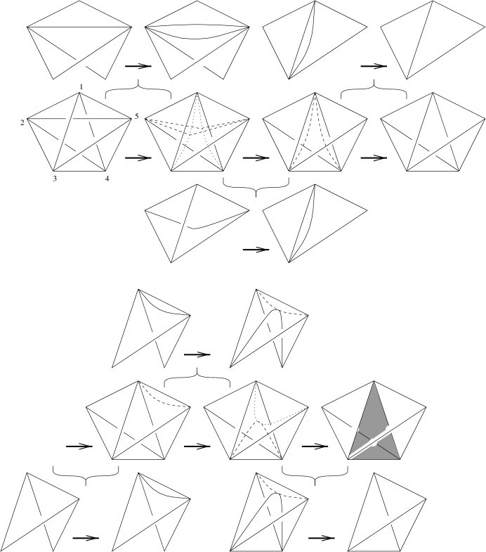
Figure 10: A Pachner move follows from cone moves

2.5

Dijkgraaf-Witten invariants. We review the Dijkgraaf-Witten invariants for 3-dimensional manifolds. In [18] Dijkgraaf and Witten gave a combinatorial definition for Chern-Simons invariants with finite gauge groups using $3$-cocycles of the group cohomology. We follow Wakui’s description [44] except we use the Pachner moves. See [44] for more detailed treatments.

Let $T$ be a triangulation of an oriented closed $3$-manifold $M$, with $a$ vertices and $n$ tetrahedra. Give an ordering to the set of vertices. Let $G$ be a finite group. Let $\phi:$ $\{$ oriented edges $\}\rightarrow G$ be a map such that

(1) for any triangle with vertices $v_{0},v_{1},v_{2}$ of $T$, $\phi(\langle v_{0},v_{2}\rangle)=\phi(\langle v_{1},v_{2}\rangle)\phi(\langle v_{0},v_{1}\rangle)$, where $\langle v_{i},v_{j}\rangle$ denotes the oriented edge, and

(2) $\phi(-e)=\phi(e)^{-1}$.

Let $\alpha:G\times G\times G\rightarrow A$, $(g,h,k)\mapsto\alpha[g|h|k]\in A$, be a $3$-cocycle with a multiplicative abelian group $A$. The $3$-cocycle condition is

$$\alpha[h|k|l]\alpha[gh|k|l]^{-1}\alpha[g|hk|l]\alpha[g|h|kl]^{-1}\alpha[g|h|k]=1.$$

Then the Dijkgraaf-Witten invariant is defined by

$$Z_{M}=\frac{1}{|G|^{a}}\sum_{\phi}\Pi_{i=1}^{n}W(\sigma,\phi)^{\epsilon_{i}}.$$

Here $a$ denotes the number of the vertices of the given triangulation, $W(\sigma,\phi)=\alpha[g|h|k]$ where $\phi(\langle v_{0},v_{1}\rangle)=g$, $\phi(\langle v_{1},v_{2}\rangle)=h$, $\phi(\langle v_{2},v_{3}\rangle)=k$, for the tetrahedron $\sigma=|v_{0}v_{1}v_{2}v_{3}|$ with the ordering $v_{0}<v_{1}<v_{2}<v_{3}$, and $\epsilon=\pm 1$ according to whether or not the orientation of $\sigma$ with respect to the vertex ordering matches the orientation of $M$.

Then one checks the invariance of this state sum under Pachner moves, see Figure 11.

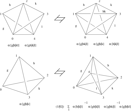
Figure 11: Pachner moves and the $3$-cocycle condition

2.6

Summary: Going up dimensions. As we reviewed the invariants in dimensions $2$ and $3$, there are two ways to go up the dimension from $2$ to $3$. One way is to consider the algebras formed by representations of quantum groups as in Turaev-Viro invariants. In this case algebra elements are regarded as vector spaces (representations) and algebras are replaced by such categories. This process is called categorification. The second way is to include a comultiplication in addition to the multiplication of an algebra as in Hopf algebra invariants and consider bialgebras (in fact Hopf algebras) instead of algebras.

Crane and Frenkel defined invariants in dimension $4$ using these ideas. We reach at the idea of the algebraic structure called Hopf categories either by (1) categorifying Hopf algebras, or (2) including comultiplications to categories of representations. The following chart represent this idea.

$$\begin{array}[]{cccc}2D&&\framebox{Associative algebras}&\\[14.22636pt] &\parbox{72.26999pt}{Categorification}\hfill\swarrow&&\searrow\hfill\parbox{72.26999pt}{Adding a comultiplication}\\[14.22636pt] 3D&\framebox{Turaev-Viro invariants}&&\framebox{Hopf algebra invariants}\\[14.22636pt] &\parbox{72.26999pt}{Adding a comultiplication}\hfill\searrow&&\swarrow\hfill\parbox{72.26999pt}{Categorification}\\[14.22636pt] 4D&&\framebox{Crane-Frenkel invariants}\end{array}$$

In the following sections we follow this idea to define invariants in dimension $4$.

We also point out here that the theories reviewed above have remarkable features in that they have direct relations between algebraic structures and triangulations via diagrams (trivalent planar graphs, or spin networks). On the one hand such diagrams appear as dual complexes through movie descriptions of duals of triangulations, and on the other hand they appear as diagrammatic representations of maps in algebras. In the following sections we explore such relations and actually utilize diagrams to prove well-defined-ness of the invariants proposed by Crane and Frenkel.

3 Pachner Moves in dimension $4$

In Section 2.2 we reviewed the Pachner moves for triangulations in dimensions $2$ and $3$ and their relations to associativity of algebras. In this section, we describe Pachner moves in dimension $4$. Relations of these moves to the Stasheff polytope was discussed in [10].

In general, an $n$-dimensional Pachner move of type $(i\rightleftharpoons j)$, where $i+j=n+2$, is obtained by decomposing the (spherical) boundary of an $(n+1)$-simplex into the union of two $n$-balls such that one of the balls is the union of $i\ \$ $n$-simplices, the other ball is the union of $j\ \$ $n$-simplices, and the intersection of these balls is an $(n-1)$-sphere. By labeling the vertices of the $(n+1)$-simplex these moves are easily expressed. For example, the table below indicates the lower dimensional Pachner moves:

$n=1$	$(1\rightleftharpoons 2)$	$(01)\rightleftharpoons(02)\cup(12)$
$n=2$	$(1\rightleftharpoons 3)$	$(012)\rightleftharpoons(013)\cup(023)\cup(123)$
	$(2\rightleftharpoons 2)$	$(012)\cup(023)\rightleftharpoons(013)\ \cup(123)$
$n=3$	$(1\rightleftharpoons 4)$	$(0123)\rightleftharpoons(0134)\cup(0234)\cup(1234)$
	$(2\rightleftharpoons 3)$	$(0123)\cup(1234)\rightleftharpoons(0124)\cup(0134)\cup(0234)$
$n=4$	$(1\rightleftharpoons 5)$	$(01234)\rightleftharpoons(01235)\cup(01245)\cup(01345)\cup(02345)\cup(12345)$
	$(2\rightleftharpoons 4)$	$(01234)\cup(01235)\rightleftharpoons(12345)\cup(01245)\cup(01345)\cup(02345)$
	$(3\rightleftharpoons 3)$	$(01234)\cup(01245)\cup(02345)\rightleftharpoons(01235)\cup(01345)\cup(12345)$

The relationship between the general Pachner move and the higher order associativity relations are explained in [10]. Next we turn to a more explicit description of the $4$-dimensional Pachner Moves.

3.1

4-dimensional Pachner moves. In this section we explain the $4$-dimensional Pachner moves. One side of a 4-dimesional Pachner move is the union of $4$-faces of a $5$-simplex (homeomorphic to a $4$-ball), and the other side of the move is the union of the rest of $4$-faces.

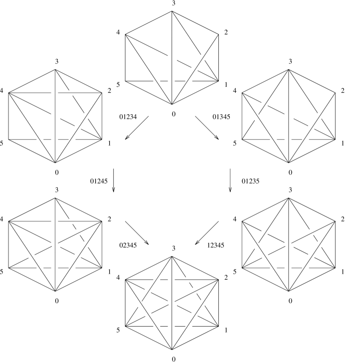
Figure 12: 4-dimensional Pachner move I

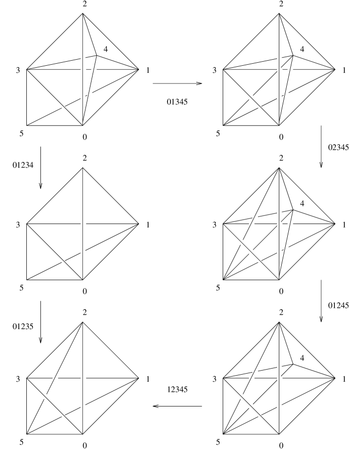
Figure 13: 4-dimensional Pachner move II

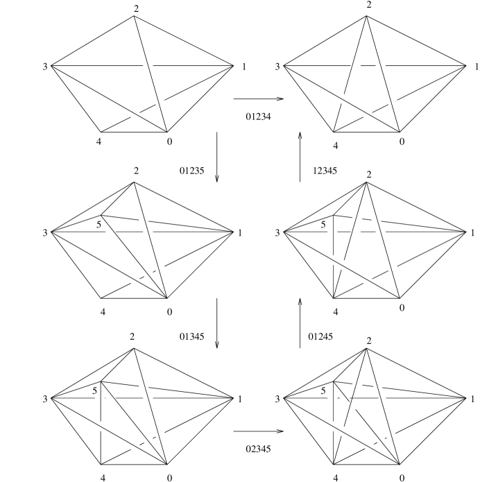
Figure 14: 4-dimensional Pachner move III

In Figures 12 13, and 14 the $(3\rightleftharpoons 3)$-move, $(2\rightleftharpoons 4)$-move, and $(1\rightleftharpoons 5)$-move are depicted, respectively. Recall here that each 3-dimensional Pachner move represents a $4$-simplex. Therefore the 3-dimensional Pachner move depicted in the top left of Figure 12, the move represented by an arrow labeled $(01234)$, represents the $4$-simplex with vertices $0$, $1$, $2$, $3$ and $4$. Then the left-hand side of Fig. 12 represents the union of three $4$-simplices $(01234)\cup(01245)\cup(02345)$. Similarly, the right-hand side of Fig. 12 represents the union of the three $4$-simplices $(01345)\cup(01235)\cup(12345)$.

3.2

Singular moves. In dimension 4, the Pachner moves can be decomposed as singular moves and lower dimensional moves. Here we define a 4-dimensional singular moves (called cone, pillow, taco moves) and show how the Pachner moves follow. This material was discussed in [10].

3.2.1

Definition (cone move). The cone move for $CW$-complexes for $4$-manifolds is defined as follows.

Suppose there is a pair of tetrahedra $(1234)_{1}$ and $(1234)_{2}$ that share the same faces $(123)$, $(124)$ and $(134)$, but have different faces $(234)_{1}$ and $(234)_{2}$, such that (1) $(234)_{1}$ and $(234)_{2}$ bound a 3-ball $B$ in the 4-manifold, (2) the union of $B$ , $(1234)_{1}$ and $(1234)_{2}$ is diffeomorphic to the $3$-sphere bounding a $4$-ball $W$ in the 4-manifold.

The situation is depicted in Figure 15 which we now explain. The left-hand-side of the Figure has two copies of tetrahedra with vertices $1$, $2$, $3$, and $4$. They share the same faces $(123)$, $(124)$, and $(134)$ but have two different faces with vertices $2$, $3$, and $4$.

Triangle	is a face of	tetrahedron
$(234)_{1}$	$\subset$	$(2348)$
$(123)_{2}$	$\subset$	$(2349)$
$(123)$	$\subset$	$(1234)_{1}$ $(1234)_{2}$ $(1237)$
$(124)$	$\subset$	$(1234)_{1}$ $(1234)_{2}$ $(1246)$
$(134)$	$\subset$	$(1234)_{1}$ $(1234)_{2}$ $(1345)$

Collapse these two tetrahedra to a single tetrahedra to get the right-hand-side of the Figure. Now we have a single tetrahedron with vertices $1$, $2$, $3$, and $4$. The face $(234)$ now is shared by three tetrahedra $(1234)$, $(2348)$, and $(2349)$ while three faces $(123)$, $(124)$, and $(134)$ are shared by two tetrahedra.

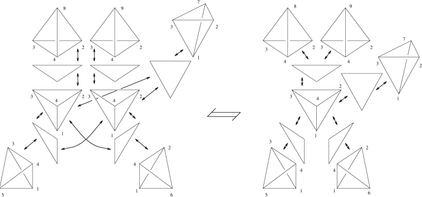
Figure 15: 4-dimensional cone move

3.2.2

Definition (taco move). Suppose we have a $CW$-complex such that there is a pair of tetrahedra $(1234)_{1}$ and $(1234)_{2}$ that share two faces $(123)$ and $(124)$ but have different faces $(134)_{1}$, $(134)_{2}$ and $(234)_{1}$, $(234)_{2}$ (of $(1234)_{1}$, $(1234)_{2}$ respectively). Suppose further that $(134)_{1}$, $(134)_{2}$, $(234)_{1}$, and $(234)_{2}$ together bound a $3$-cell $B$ and $(1234)_{1}$, $(1234)_{2}$, and $B$ bounds a $4$-cell. Then collapse this $4$-cell to get a single tetrahedron $(1234)$. As a result $(134)_{1}$ (resp. $(234)_{1}$) and $(134)_{2}$ (resp. $(234)_{2}$) are identified. This move is called the taco move.

3.2.3

Definition (pillow move). Suppose we have a $CW$-complex such that there is a pair of tetrahedra sharing all four faces cobounding a $4$-cell. Then collapse these tetrahedra to a single tetrahedron. This move is called the pillow move.

3.2.4

Lemma. The $(3\rightleftharpoons 3)$ Pachner move is described as a sequence of cone moves, pillow moves, taco moves, and $3$-dimensional Pachner moves.

Proof. The proof can be facilitated by following the Figures 16 through 24. Figure 16 is a preliminary sketch that indicates in dimension 3 the methods of the subsequent figures. It illustrates that the $(2\rightleftharpoons 3)$-move in dimension 3 can be interpreted in terms of the $(2\rightleftharpoons 2)$-move via a non-generic projection. The thick vertical line on the left-hand-side of the figure is the projection of the triangle along which the two tetrahedra are glued. The thick horizontal line on the right is the projection of one of the three triangles that are introduced on the right-hand-side of the move. The other two triangles project to fill the lower right quadrilateral. The dotted lines indicate that some edges in the figure will project to these lines. Some information is lost during the projection process, but at worst, the projected figures serve as a schematic diagram of the actual situation.

Figure 16: Projecting the (2,3)-move

In Fig. 17 the union of the three 4-simplices $(ABCDE)$, $(ACDEF)$, and $(ABCEF)$ is illustrated; these share the triangle $(ACE)$ which is shaded in figure. The union forms the left-hand-side of the of the $(3\rightleftharpoons 3)$-move. Let $P$ denote this union. In the top of Fig. 18, the triangle $(ACE)$ has been projected to the thick line $(EAC)$. At the bottom of Fig. 18, the 4-simplex $(ACEF)$ has been split into simplices $(ACEF)_{1}$ and $(ACEF)_{2}$ by a cone move. The cone move is illustrated in this projection, and the schematic resembles the cone move in dimension 3 as is seen on the bottom left of the figure. Thus $(ACEF)_{1}$ and $(ACEF)_{2}$ share the same faces $(ACF)$, $(AEF)$ and $(CEF)$ but have different faces $(ACE)_{1}$ and $(ACE)_{2}$. The face $(ACE)_{1}$ is shared with $(ABCE)$ and the face $(ACE)_{2}$ is shared with $(ACDE)$ respectively.

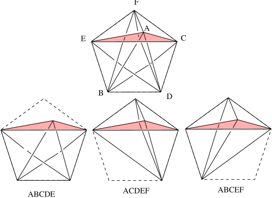
Figure 17: The left-hand-side of the (3,3)-move

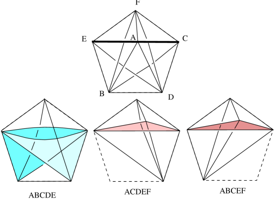
Figure 18: Splitting the tetrahedron $(ACEF)$ via a cone move

After the splitting, $P$ consists of three $4$-polytopes, $\tau^{1}_{j}$, $j=1,2,3$. Here the polytope $\tau^{1}_{1}$ is bounded by tetrahedra $(ABCD)$, $(ABDE)$, $(ABCE)$, $(ACDE)$, $(BCDE)$, $(ACEF)_{1}$, and $(ACEF)_{2}$. The polytope $\tau^{1}_{2}$ is bounded by tetrahedra $(ABCE)$, $(ABEF)$, $(ACEF)_{1}$, $(ABCF)$, and $(BCEF)$. The polytope $\tau^{1}_{3}$ is bounded by tetrahedra $(ACDE)$, $(ACEF)_{2}$ $(ACDF)$, $(ADEF)$, and $(CDEF)$. The polytope $\tau^{1}_{1}$ corresponds to $(ABCDE)$ and it is illustrated on the left bottom of Fig. 18 (labeled $(ABCDE)$ to indicate the correspondence). On the bottom right of the figure, we see the polytope $\tau^{1}_{2}$ labeled $(ABCEF)$. In the bottom center of the figure the polytope $\tau^{1}_{3}$ labeled $(ACDEF)$ to indicate its antecedent. Our first work will be on $\tau^{1}_{1}$ and $\tau^{1}_{3}$.

Next perform a Pachner move to the pair of tetrahedra $(ACDE)\cup(ACEF)_{2}$ sharing the face $(ACE)_{2}$. Note that these two tetrahedra are shared by $\tau^{1}_{1}$ and $\tau^{1}_{3}$ so that the Pachner move we perform does not affect $\tau^{1}_{2}$. Thus we get three $4$-cells $\tau^{2}_{j}$, $j=1,2,3$, where $\tau^{2}_{2}=\tau^{1}_{2}$, and $\tau^{2}_{1}$ is bounded by $(ABCD)$, $(ABDE)$, $(ABCE)$, $(BCDE)$, $(ACEF)_{1}$, $(ACDF)^{\prime}$, $(ADEF)^{\prime}$, and $(CDEF)^{\prime}$. Here $(ACDF)^{\prime}$, $(ADEF)^{\prime}$, and $(CDEF)^{\prime}$ denote new tetrahedra obtained as a result of performing a Pachner move to $(ACDE)\cup(ACEF)_{2}$. Then the last polytope $\tau^{2}_{3}$ is bounded by $(ACDF)^{\prime}$, $(ADEF)^{\prime}$, and $(CDEF)^{\prime}$ that are explained above, and $(ACDF)$, $(ADEF)$, $(CDEF)$ that used to be faces of $\tau^{1}_{3}$.

The $(2\rightleftharpoons 3)$-move to $(ACDE)\cup(ACEF)$ is illustrated in Fig. 19. In the upper left the the 4-cell $\tau^{2}_{1}$ is shown while $\tau^{2}_{3}$ is shown on the upper right. In the lower part of the figure the three new tetrahdera $(ACDF)^{\prime}$ $(ADEF)^{\prime}$, and $(CDEF)^{\prime}$ are illustrated.

Figure 19: Performing a $(2,3)$-move to $(ACDE)\cup(ACEF)$

Then we can collapse $\tau^{2}_{3}$ to the tetrahedra $(ACDF)$, $(ADEF)$, $(CDEF)$ as in the following 3 paragraphs and 2 tables.

The polytope $\tau^{2}_{3}$ is a $4$-cell bounded by $(ACDF)$, $(ADEF)$, $(CDEF)$, $(ACDF)^{\prime}$, $(ADEF)^{\prime}$, and $(CDEF)^{\prime}$. The incidence relations for these tetrahdra are indicated in the next table. Also see the top two rows of Fig. 20.

Triangles	are faces of	tetrahedra
$\left\{\begin{array}[]{c}(ACD)\\ (ACF)\end{array}\right\}$	$\subset$	$(ACDF)\cup(ACDF)^{\prime}$
$\left\{\begin{array}[]{c}(ADE)\\ (AEF)\end{array}\right\}$	$\subset$	$(ADEF)\cup(ADEF)^{\prime}$
$\left\{\begin{array}[]{c}(CDE)\\ (CEF)\end{array}\right\}$	$\subset$	$(CDEF)\cup(CDEF)^{\prime}$
$(ADF)$	$\subset$	$(ACDF)\cup(ADEF)$
$(DEF)$	$\subset$	$(ADEF)\cup(CDEF)$
$(CDF)$	$\subset$	$(ACDF)\cup(CDEF)$
$(ADF)^{\prime}$	$\subset$	$(ACDF)^{\prime}\cup(ADEF)^{\prime}$
$(DEF)^{\prime}$	$\subset$	$(ADEF)^{\prime}\cup(CDEF)^{\prime}$
$(CDF)^{\prime}$	$\subset$	$(ACDF)^{\prime}\cup(CDEF)^{\prime}$

Figure 20: Performing a taco move to the pair $(CDEF)$ and $(CDEF)^{\prime}$

Then perform the taco move to the pair $(CDEF)$ and $(CDEF)^{\prime}$ that share two faces $(CDE)$ and $(CEF)$. This move is illustrated at the bottom of Fig. 20. Then the faces $(CDF)$ and $(CDF)^{\prime}$, $(DEF)$ and $(DEF)^{\prime}$ are identified after the move respectively. The result is a $4$-cell bounded by $(ACDF)$, $(ADEF)$, $(ACDF)^{\prime}$, and $(ADEF)^{\prime}$. (Precisely speaking these tetrahdera share new faces so that we should use the different labels, but adding a new layer of labels here will cause more confusion than leveing the old labels intact). The incidence relations among the triangles and the tetrahedra are summarized in the next table.

Triangles	are faces of	tetrahedra
$\left\{\begin{array}[]{c}(ACD)\\ (ACF)\\ (CDF)\end{array}\right\}$	$\subset$	$(ACDF)\cup(ACDF)^{\prime}$
$\left\{\begin{array}[]{c}(ADE)\\ (AEF)\\ (DEF)\end{array}\right\}$	$\subset$	$(ADEF)\cup(ADEF)^{\prime}$
$(ADF)$	$\subset$	$(ACDF)\cup(ADEF)$
$(ADF)^{\prime}$	$\subset$	$(ACDF)^{\prime}\cup(ADEF)^{\prime}$

The cone move to $(ADEF)$ and $(ADEF)^{\prime}$ (which is illustrated schematically in Fig. 21) followed by the pillow move to $(ACDF)$ and $(ACDF)^{\prime}$ collapses $\tau^{2}_{3}$ to $(ACDF)\cup(ADEF)\cup(CDEF)$ as claimed.

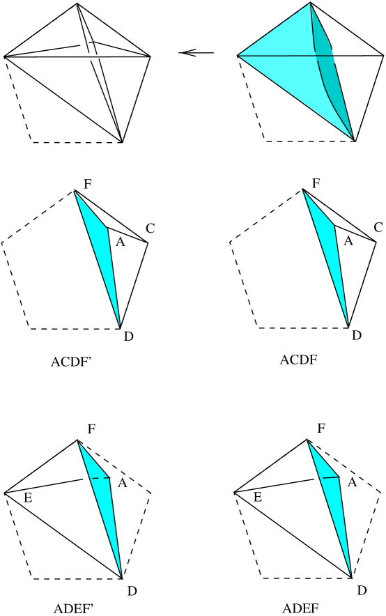
Figure 21: Performing a cone move to the pair $(ADEF)$ and $(ADEF)^{\prime}$

Thus we get two polytopes $\tau^{2}_{1}$ and $\tau^{2}_{2}$. Next perform a Pachner move to $(ABCE)\cup(ACEF)_{1}$ which shares $(ACE)_{1}$. As a result we get three new tetrahedra $(ABEF)^{\prime}\cup(ABCF)^{\prime}\cup(BCEF)^{\prime}$. The $(2\rightleftharpoons 3)$-move is illustrated in Fig. 22; the labels on the polytopes indicate their antecendents.

Thus we obtain $\tau^{3}_{1}$ bounded by $(ABCD)$, $(ABDE)$, $(BCDE)$, $(ACDF)$, $(ADEF)$, $(CDEF)$, $(ABEF)^{\prime}$, $(ABCF)^{\prime}$, and $(BCEF)^{\prime}$, and $\tau^{3}_{2}$ bounded by $(ABEF)$, $(ABCF)$, $(BCEF)$, and $(ABEF)^{\prime}\cup(ABCF)^{\prime}\cup(BCEF)^{\prime}$.

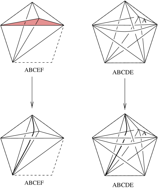
Figure 22: Performing a $(2,3)$-move to the pair $(ABCE)$ and $(ACEF)_{1}$

Hence we now can collapse $\tau^{3}_{2}$ to the tetrahedra $(ABEF)$, $(ABCF)$, and $(BCEF)$ in the same manner as we did to $\tau^{2}_{3}$. The collapsing is indicated in Fig. 23. The result is a single polytope $\tau^{4}$ resulted from $\tau^{3}_{1}$ which has the same boundary tetrahedra as those of the left hand side of the 4-dimensional Pachner move. Figure 23 indicates the resulting polytope at the bottom of the figure. In Fig. 24 the 3-dimensional boundary is illustrated. Notice the following: (1) triangle (ACE) is no longer present; (2) among the nine tetrahedra illustrated, neither triangle $(ACE)$ nor triangle $(BDF)$ appears; (3) these are all of the tetrahedral faces of the 5 simplex that contain neither $(ACE)$ nor $(BDF)$. Thus we can apply the same method starting with $(BDF)$ to get to this polytope. This proves that $(3\rightleftharpoons 3)$-move is described as a sequence of singular moves (cone, taco, and pillow moves) and Pachner moves.

Figure 23: Collapsing to a single polytope

Figure 24: The tetrahedral faces of the middle stage

$\Box$

3.2.5

Lemma. The $(2\rightleftharpoons 4)$-move is described as a sequence of cone moves, pillow moves, taco moves, and $3$-dimensional Pachner moves.

Proof. We use the following labeling for the $(2\rightleftharpoons 4)$-move in this proof:

$$(ABCDE)\cup(ABCEF)\rightleftharpoons(ABCDF)\cup(ABDEF)\cup(ACDEF)\cup(BCDEF).$$

Perform a $(3\rightleftharpoons 3)$-move (which was proved to be a sequence of the singular moves in the preceeding Lemma) to $(ABCDF)\cup(ABDEF)\cup(ACDEF)$ to get $(ABCDE)^{\prime}\cup(ABCEF)^{\prime}\cup(ACDEF)^{\prime}$. Then the polytope now consists of $(ABCDE)^{\prime}$, $(ABCEF)^{\prime}$, $(ACDEF)^{\prime}$, and $(ACDEF)$.

Perform a Pachner move to the tetrahedra $(ACDF)\cup(ADEF)\cup(CDEF)$, that are shared by $(ACDEF)^{\prime}$ and $(ACDEF)$, to get $(ACDE)^{\prime}\cup(ACEF)^{\prime}$.

This changes $(ACDEF)^{\prime}\cup(ACDEF)$ to a $4$-cell bounded by $(ACDE)$, $(ACDE)^{\prime}$, $(ACEF)$, and $(ACEF)^{\prime}$. The cone move followed by the pillow move collapses this polytope yielding $(ABCDE)\cup(ABCEF)$, the left-hand-side of the $(2\rightleftharpoons 4)$-move. $\Box$

3.2.6

Lemma. The $(1\rightleftharpoons 5)$-move is described as a sequence of cone moves, pillow moves, taco moves, and $3$-dimensional Pachner moves.

Proof. We use the following labelings:

$$(ABCDE)\rightleftharpoons(ABCDF)\cup(ABCEF)\cup(ABDEF)\cup(ACDEF)\cup(BCDEF).$$

Perform the $(3\rightleftharpoons 3)$-move to $(ABCDF)\cup(ABDEF)\cup(BCDEF)$ to get $(ABCDE)\cup(ABCEF)^{\prime}\cup(ACDEF)^{\prime}$.

The $4$-simplices $(ACDEF)$ and $(ACDEF)^{\prime}$ share all their tetrahedral faces except $(ADEF)$ (and $(ADEF)^{\prime}$). Perform a $(1\rightleftharpoons 3)$-move to each of these shared tetrahedra to get $4$-cells bounded by copies of $(ADEF)$ sharing all the $2$-faces. Thus the pillow moves will collapse $(ACDEF)$ and $(ACDEF)^{\prime}$. The same argument collapses $(ABCEF)\cup(ABCEF)^{\prime}$ to get the left-hand-side of the $(1\rightleftharpoons 5)$-move. $\Box$

3.2.7

Remark. In [13] Crane and Frenkel proposed constructions of $4$-manifold quantum invariants using Hopf categories. Hopf categories generalize the definition of Hopf algebra to a categorical setting in the same way that modular categories generalize modules. One of the conditions in their definition is called the coherence cube which generalizes the compatibility condition of Hopf algebras between mutiplication and comutiplication (See Section 8). They showed that this condition corresponds to the cone move. Thus Lemmas in this section can be used to prove the well-definedness of invariants they proposed by showing that their definition is invariant under Pachner moves.

4 Triangulations and Diagrams

In dimension 3, quantum spin networks are used on the one hand to provide calculations of identities among representations of quantum groups [9]. On the other hand they are cross sections of the dual complex of a triangulated 3-manifold (see Section 2.2).

In this section, we use similar graphs to relate them to the dual complex of triangulated 4-manifold. We begin the discussion on the local nature of triangulated 4-manifolds near 2-dimensional faces.

4.1

Graphs, 2-complexes, and triangulations. Let $\Phi$ be a triangulation of an oriented closed $4$-manifold $M$. In this section we associate graphs to triangulations and their duals.

4.1.1

Definition. The dual complex $\Phi^{*}$ of $\Phi$ is defined as follows. Pick a vertex $v$ of $\Phi^{*}$ in the interior of each $4$-simplex of $\Phi$. Connect two vertices $v_{1}$ and $v_{2}$ of $\Phi^{*}$ if and only if the corresponding $4$-simplices of $\Phi$ share a $3$-face. Thus each edge of $\Phi^{*}$ is dual to a tetrahedron of $\Phi$. Edges $e_{1},\cdots,e_{k}$ of $\Phi^{*}$ bound a face $f$ if and only if the corresponding tetrahedra share a $2$-face of $\Phi$. A set of $2$-faces $f_{1},\cdots,f_{k}$ of $\Phi^{*}$ bounds a $3$-face (a polyhedron) if and only if the corresponding faces of $\Phi$ share an edge of $\Phi$. Finally a set of $3$-faces of $\Phi^{*}$ bounds a $4$-face if and only if the corresponding edges of $\Phi$ share a vertex. Thus $\Phi^{*}$ gives a CW-complex structure to the $4$-manifold.

4.1.2

Definition. Let $\Phi$ be a triangulation of a $4$-manifold $M$, and let $\Phi^{*}$ be the dual complex. Each $3$-face of $\Phi^{*}$ is a polytope. Choose a triangulation of each $3$-face into tetrahedra so that it defines a triangulation of the $3$-skeleton of $\Phi^{*}$. We require that such a triangulation does not have interior vertices in the $2$-faces of $\Phi^{*}$. Thus the restriction on each $n$-agonal $2$-face consists of $(n-2)$ triangles. Such a choice of triangulation is called a $3$-face triangulation (a triangulation for short) of $\Phi^{*}$. A $3$-face triangulation is denoted by $\Phi^{!}$.

4.1.3

Definition (Carrier Surface). In each tetrahedron of the triangulation $\Phi$, we embed the dual spine to the tetrahedron. The intersection of the dual spine with a triangular face is a graph consisting of a 3-valent vertex with edges intersecting the edges of the tetrahedron. There is a vertex in the center of the 2-complex at which four edges (corresponding to the faces of the tetrahedron) and six faces (corresponding to the edges) intersect. The union (taken over all tetrahedra in the triangulated 4-manifold) of these 2-complexes form a 2-complex, $C$, that we call the carrier surface. Let us examine the incidence relations of the carrier surface along faces and edges of the triangulation.

Consider a 2-face, $f$, of the triangulation $\Phi$. Suppose that $n$ tetrahedra are incident along this triangle $f$. Then the dual face $f^{*}$ is an $n$-gon. The 4-manifold in a neighborhood of the face $f$ looks like the Cartesian product $f\times f^{*}$. The carrier surface in this neighborhood then appears as $Y\times X_{n}$ where $X_{n}$ is the 1-complex that consists of the cone on $n$-vertices (i.e., the $n$-valent vertex), and $Y$ is the graph that underlies that alphabet character (a neighborhood of a trivalent vertex). For example $X_{2}$ is an interval, $X_{3}=Y$, $X_{4}=X$, etc. We can think of $X_{n}$ being embedded in $f^{*}$ with the edges of $X_{n}$ intersecting the centers of the edges of $f^{*}$ and the vertex of $X_{n}$ lying at the “center” of $f^{*}$ (i.e. we may assume that $f^{*}$ is a regular polygon).

Consider an edge, $e$, of $\Phi$, and the 3-cell, $e^{*}$, that is dual to $e$. The faces of $e^{*}$ are $n$-gons, $f^{*}$, that are dual to the triangular faces, $f$, which are incident to $e$. The carrier surface intersects a face $f^{*}$ in the graph $X_{n}$. The carrier surface intersects $e^{*}$ in a 2-complex that is the cone on the union of the $X_{n}$ where the union is taken over all the faces of $e^{*}$.

The situation is depicted in Fig. 25 in which three tetrahedra intersect along a triangular face. On the right hand side of the figure, we illustrate a graph movie. The two graphs that are drawn there represent the intersection of the carrier complex with the boundary of $f\times f^{*}$. In a neighborhood of this face the carrier complex looks like $Y\times Y$. In this and subsequent figures, the vertices that are labeled with open circles correspond to the dual faces $f^{*}$. In this figure, three such circled vertices appear since the dual face appears on each of the duals to the three edges.

4.2

Faces and diagrams. Suppose that the face $(012)$ of a triangulation of a $4$-manifold is shared by three tetrahedra $T_{i}$, $i=1,2,3$. Take a neighborhood $N$ of the face $(012)$ in the $3$-skeleton of the triangulation such that $N\cap T_{i}$ is diffeomorphic to $(012)\times I$ for each $i=1,2,3$.

In Fig. 25 the projection of a neighborhood $N$ of the face $(012)$ is depicted in $3$-space. Denote by $0^{\prime}$, $0^{\prime\prime}$, $0^{\prime\prime\prime}$ the vertices obtained from the vertex $0$ by pushing it into $T_{i}$, $i=0,1,2,$ respectively (they are depicted in Fig. 25). Similar notation is used for the other vertices.

The graph movie for $N$ is constructed as follows. Regard $N$ as a $3$-dimensional polyhedral complex consisting of the following faces: $(0^{\prime}1^{\prime}2^{\prime})$, $(0^{\prime\prime}1^{\prime\prime}2^{\prime\prime})$, $(0^{\prime\prime\prime}1^{\prime\prime\prime}2^{\prime\prime\prime})$, $(011^{\prime}0^{\prime})$, $(010^{\prime\prime}1^{\prime\prime})$, $(010^{\prime\prime\prime}1^{\prime\prime\prime})$, $(122^{\prime}1^{\prime})$, $(122^{\prime\prime}1^{\prime\prime})$, $(122^{\prime\prime\prime}1^{\prime\prime\prime})$, $(200^{\prime}2^{\prime})$, $(200^{\prime\prime}2^{\prime\prime})$, $(200^{\prime\prime\prime}2^{\prime\prime\prime})$. Then trivalent vertices are assigned to the middle points of the triangular faces $(0^{\prime}1^{\prime}2^{\prime})$, $(0^{\prime\prime}1^{\prime\prime}2^{\prime\prime})$, $(0^{\prime\prime\prime}1^{\prime\prime\prime}2^{\prime\prime\prime})$, and the middle points of the edges $(01)$, $(12)$, $(20)$. These are connected by segments as indicated in the figure where this 1-complex is depicted in two parts. The middle point in the interior of $N$ is the cone point of this $1$-dimensional complex. Within $N$ we have an embedding of the Cartesian product $Y\times Y$ where $Y$ represents the obvious graph with one trivalent vertex. The graphs on the right of Fig. 25 represent portions of the boundary of $Y\times Y$. The space $Y\times Y$ is indicated in Fig. 26 in which the subspace $\circ\times Y$, where $\circ$ denotes a vertex, is indicated as a fat vertex times $Y$. The labels on the Figure will be explained in Section  6.1.1 and Fig. 34.

Below (Sections 6.4 and 8) we will relate these spin networks to cocycle conditions in a specific Hopf category. In this way, we will obtain a direct connection among these structures.

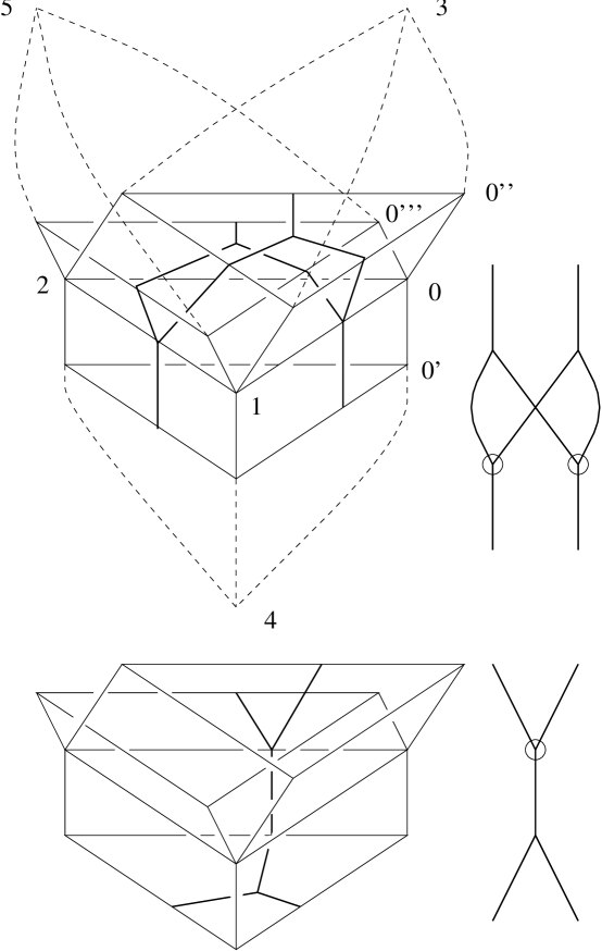
Figure 25: Graphs and triangulations around a face

Figure 26: The product space YxY

4.2.1

Defintion. We perturb the carrier surface to construct a 2-dimensional complex that has the following properties:

1. The vertices of the complex all have valence 4 or valence 6.

2. Exactly three sheets meet along an edge;

3. The set of edges can be partitioned into two subsets; we color the edges accordingly.

4. A valence 4 vertex has 4 edges of the same color incident to it;

5. A valence 6 vertex has 3 edges of each color incident to it.

6. Thus, the 2-complex has a tripartite graph as its 1-complex and a bipartition on the set of edges.

Such a 2-complex will be called a perturbed carrier.

Figure 27: A neighborhood of an edge whose dual is a cube

4.2.2

Lemma. A perturbed carrier can be constructed from the carrier surface by means of a 3-face triangulation.

Proof. Consider a 3-face triangulation; recall this is a triangulation of the dual 3-cells of the triangulation $\Phi$, and a 3-face is the dual to an edge $e^{*}$. A $n$-agonal face of $e^{*}$ is divided into $(n-2)$ triangles. The graph $X_{n}$ in the $n$-agonal face is replaced with the dual to the triangulation. In $e^{*}$, the cone on the union of the $X_{n}\/$s is replaced by the union of the duals to the tetrahedra in the triangulation. These are the surfaces with 6 faces, 1 vertex, and 4 edges; they glue together in $e^{*}$ to form the subcomplex in which all of the vertices have one color. An example is illustrated in Fig. 27 in which the dual of an edge is a cube.

The vertices that have two different colored edges incident to them are found on the triangular faces of the 3-face triangulation. Three of the edges are coming from the dual face, the other three edges are coming from the dual complex of the original tetrahedra. The local structure at the 6-valent vertices was explained in detail above. This completes the proof. $\Box$

4.2.3

Definition. A graph movie is a sequence of graphs that appear as cross sections of a portion of the perturbed carrier when a height function is chosen, such that the stills of movies are graphs having trivalent (circled and uncircled) vertices and between two stills, the movie changes in one of the following ways:

1. The change of the movie at a face (a $6$-valent vertex of a carrier surface) is as defined above (the change of graphs shown in Fig. 25).

2. The change of the movie at a $4$-valent vertex is as depicted in Fig. 32 bottom.

3. The changes of the movie at critical points of edges and faces of the carrier surface is generic. They are depicted in Fig. 28.

Figure 28: Some elementary changes of graph movies

In the graphs we use circled vertices and uncircled vertices. These are cross section of two types of edges. In the figures of carrier surfaces (Fig. 38, 39, and 27), the edges corresponding to circled vertices are depicted by thin tubes. The graph movie defined here includes definitions given above (which are clearly equivalent). The graph movie allows us to view the perturbed carrier via a sequence of 2-dimensional cross-sections whereas the carrier surface itself does not embed in 3-dimensional space.

4.3

Taco moves and graph movies. Herein we directly relate the graph movies to the taco move. In Figs. 29 and 30 the left-hand-side and the right-hand-side of the taco move are depicted, respectively. In each figure, the underlying union of tetrahedra remains unchanged from frame to frame. Instead the thick lines change as follows. Consider the $(i,j)\/$th entry of the figure to be that illustration in the $i\/$th row $j\/$th column. Going from the $(i,1)\/$st entry to the $(i,2)\/$nd entry, the graphs change by one of the graph movie changes (either going across $Y\times Y$ or going across tetrahedra). There is no change from the $(i,2)\/$nd entry to the $(i+1,1)\/$st entry. In these figures thick lines indicate the graph that was defined in Section 4.2. The transitions between the two entries on the same row may be visualized by means of a cross-eyed stereo-opsis. Place a pen in the center of the figure, and move the pen towards your face while keeping it in focus. The two images on the left and right should converge into one with the thick lines popping out of the plane of the paper. In this way, the difference between the figures can be experienced directly.

Observe that the differences in the graphs are illustrated as well in the Fig. 36 which illustrates the graph movies for the cocycle conditions and which is obtained by purely algebraic information. The time elapsed version of the graph movie for the taco move is illustrated in Fig. 38 and Fig. 39. Similar diagrams can be drawn for the cone move and the pillow move and in this way a direct correspondence can be obtained among the moves, the cocycle conditions, and the axioms of a Hopf category (Section 8). The taco, cone, and pillow moves all correspond to the first coherence cube. The correspondence among these moves should not be surprising since all of these moves correspond to splitting a tetrahedron open (the higher dimensional analogue of the coherence relation between multiplication and comultiplication).

Figure 29: The taco move and graph movie, left-hand-side

Figure 30: The taco move and graph movie, right-hand-side

5 Cocycles and cocycle conditions

In this section, we list cocycles and their equalities that will be used in the following sections. These cocycles are given in [17] in relation to Hopf categories (See Section 8). Some non-trivial examples are given therein. First, we mention that two of the cocycle conditions are depicted in Figs. 36 and 37 as relations to graph movies where the edges of the graph have been colored with pairs of group elements and dual group elements. These graph movies correspond to the dual graphs that correspond to the taco move (Fig. 29 and 30). The coloring will be explained in the subsequent section.

Let $G$ be a finite group and $K^{\times}$ be the multiplicative group of a field $K$. Let $C_{n,m}=C_{n,m}(G,K^{\times})$ denote the abelian group of all functions from $G^{n}\times\hat{G}^{m}$ to $K^{\times}$ where

$$\hat{G}=\{\hat{g}:G\rightarrow K|g\in G,\hat{g}(h)=1\;\mbox{if}\;g=h,\hat{g}(h)=0\;\mbox{if}\;g\neq h\}.$$

We need the following functions (called cocycles if they satisfy the conditions given in the next section).

• $\alpha(g,k,m;\hat{n})\in C_{3,1}$,

• $\beta(g;\hat{i},\hat{j},\hat{k})\in C_{1,3}$,

• $\phi(g,k;\hat{m},\hat{n})\in C_{2,2}$.

5.1

Cocycle conditions. The following are called the cocycle conditions [17].

• $\alpha(k,m,p;\hat{q})\alpha(g,km,p;\hat{q})\alpha(g,k,m;\widehat{pqp^{-1}})$

  $=\alpha(gk,m,p;\hat{q})\alpha(g,k,mp;\hat{q})$

• $\beta(g;\hat{j},\hat{k},\hat{\ell})\beta(g;\hat{i},\widehat{jk},\hat{\ell})\beta(g;\hat{i},\hat{j},\hat{k})$

  $=\beta(g;\hat{ij},\hat{k},\hat{\ell})\beta(g;\hat{i},\hat{j},\widehat{k\ell})$,

• $\alpha(g,k,m;\hat{p})\alpha(g,k,m;\hat{q})\phi(k,m;\hat{p},\hat{q})\phi(g,km;\hat{p},\hat{q})$

  $=\phi(g,k;\widehat{mpm^{-1}},\widehat{mqm^{-1}})\phi(gk,m;\hat{p}\hat{q})\alpha(g,k,m;\widehat{pq})$,

• $\phi(g,k;\hat{p},\hat{r})\phi(g,k;\widehat{pr},\hat{s})\beta(gk;\hat{p},\hat{r},\hat{s})$

  $=\beta(g;\widehat{kpk^{-1}},\widehat{krk^{-1}},\widehat{ksk^{-1}})\beta(k;\hat{p},\hat{r},\hat{s})\phi(g,k;\hat{r},\hat{s})\phi(g,k;\hat{p},\widehat{rs})$.

5.2

Cocycle symmetries. In addition to the above cocycle conditions, we will suppose that the cocycles satisfy some equations that correspond to the symmetries of tetrahedra and of the space $Y\times Y$. The imposition of such conditions will be sufficient to construct an invariant. We do not know if the symmetry conditions are necessary. (They may be satisfied automatically for certain cocycles, or the invariants may be defined without symmetry conditions.)

5.2.1

Definition. The following are called the cocycle symmetries.

• $\alpha(g,k,m;\hat{n})=\alpha(g^{-1},gk,m;\hat{n})^{-1}$

  $=\alpha(gk,k^{-1},km;\hat{n})^{-1}=\alpha(g,km,m^{-1};\hat{\ell})^{-1},$

  where $\ell=mnm^{-1}$.

• $\phi(g,k;\hat{m},\hat{\ell})=\phi(g^{-1},gk;m,\ell)^{-1}=\phi(gk,k^{-1};kmk^{-1},k\ell k^{-1})^{-1}$

  $=\phi(g,k;m\ell,\ell^{-1})^{-1}=\phi(g,k;m^{-1},m\ell^{-1})^{-1}.$

• $\beta(g;\hat{h},\hat{\ell},\hat{n})=\beta(g;\widehat{h^{-1}},\widehat{h\ell},\hat{n})^{-1}$

  $=\beta(g;\widehat{h\ell},\widehat{\ell^{-1}},\widehat{\ell n})^{-1}=\beta(g;\hat{h},\hat{\ell},\widehat{n^{-1}})^{-1}.$

6 Labels, weights, and the partition function

6.1

Labeling. Let $\Phi$ denote a triangulation of the $4$-manifold $M$, and let $\Phi^{*}$ denote the dual complex. Each $3$-face of $\Phi^{*}$ is a polytope that corrresponds to an edge of $\Phi$. Choose a triangulation of the $3$-skeleton of $\Phi^{*}$. There are no interior vertices in the $2$-faces of $\Phi^{*}$. Thus the restriction on each polygonal $2$-face consists of $(n-2)$ triangles. As before, such a choice of triangulation is called a $3$-face triangulation of $\Phi^{*}$. A $3$-face triangulation is denoted by $\Phi^{!}$.

When an order, ${\cal O}$, is fixed for the vertex set, ${\cal V}$, we define the orientation of dual edges as follows. A vertex of $\Phi^{*}$ is a $4$-simplex of $\Phi$ whose vertices are ordered. Then $4$-simplices are ordered by lexicographic ordering of their vertices. This gives an order on vertices of $\Phi^{*}$, giving orientations of edges of $\Phi^{*}$. Orientations of edges of $\Phi^{!}$ are ones that are compatible with the above orientation.

6.1.1

Definition. A labeling (or color) of $\Phi$ with oriented edges with respect to a finite group $G$ is a function

$$S_{0}:{\cal ET}\rightarrow{\cal G}$$

where ${\cal G}=\{(g,\hat{h})\in G\times\hat{G}\}$ and

$${\cal ET}=\{(e,t)\in{\cal E}\times{\cal T}|e\subset t\}.$$

Here ${\cal E}$ denotes the set of oriented edges, and ${\cal T}$ is the set of tetrahedra. We require the following compatibility condition.

If $(e_{1},e_{2},-e_{3})$ forms an oriented boundary of a face of a tetrahedron $t$, $S_{0}(e_{1},t)=(k,\hat{\ell})$, and $S_{0}(e_{2},t)=(g,\hat{h})$, then $S_{0}(e_{3},t)=(m,\hat{n})$, where $m=gk$, $n=\ell$, and $k^{-1}hk=\ell$. We call this rule the local rule of colors at a triangle (or simply a local rule). The situation is depicted on the left of Fig. 31.

When an order of vertices is given, the edges are oriented by ascending order of vertices (if the vertices $v$ and $w$ of an edge have the order $v<w$, then the edge is oriented from $v$ to $w$). However in this definition the order on vertices is not required, although orientations on edges are required. For an oriented edge $e$, the same edge with the opposite orientation is denoted by $-e$. Consider the edge $e_{2}$ on the left of Fig. 31, and reverse the orientation of $e_{2}$ to get $-e_{2}$. Then the color of $-e_{2}$ is required to be $S(-e_{2},t)=(g^{-1},\widehat{gk\ell k^{-1}g^{-1}})$ where $S(e_{2},t)=(g,\widehat{k\ell k^{-1}})$ as depicted in the figure. In other words, the color for an edge with reversed orientation is defined to satisfy the local requirement of the left of Fig. 31.

Figure 31: Rules of cocycle colors

We often use sets of non-negative integers to represent simplices of $\Phi$. For example, fix a $3$-face (or tetrahedron) $T$ of $\Phi$. Let $0$, $1$, $2$, and $3$ denote the vertices of $T$. For a pair of an oriented edge $(01)$ and a tetrahedron $T=(0123)$ a labeling assigns a pair $(g,\hat{h})$ which we sometimes denote by $S_{0}(01|0123)=S_{0}((01),(0123))$. When a total order is fixed, the integers are assumed to have the compatible order ($0<1<2<3$).

Figure 32: Weight for tetrahedra

Figure 33: Symmetry of colors of a tetrahedron

We will show (Lemma 6.1.5) that there is a coloring of each tetrahedron satisfying the local rule. Furthermore, we will show that changing the orientations of edges of a colored tetrahedron results in a unique coloring.

6.1.2

Definition. A labeling (or color) of $\Phi^{!}$ with oriented dual edges is a function

$$S^{!}:{\cal EP^{!}}\rightarrow{\cal G}$$

where

$${\cal EP^{!}}=\{(p,e)\in{\cal P^{*}}\times{\cal E^{!}}|e\subset p\}.$$

Here ${\cal E^{!}}$ (resp. ${\cal P^{*}}$ ) denotes the set of oriented edges (resp. 3-polytopes) of $\Phi^{!}$ (resp. $\Phi^{*}$). The following compatibility conditions are required.

If $(e_{1},e_{2},-e_{3})$ form an oriented boundary of a face of a tetrahedron $t$ of $\Phi^{!}$, then the first factors of colors (group elements) coincide, and if they are $S^{!}(e_{1},t)=(g,\hat{l})$, and $S^{!}(e_{2},t)=(g,\hat{k})$, then $S^{!}(e_{3},t)=(g,\hat{h})$, where it is required that $h=kl$.

When an order of vertices is given, the edges are oriented by ascending order of vertices as before. Consider the edge $e_{2}$ in the Fig. 31 right, and reverse the orientation of $e_{2}$ to get $-e_{2}$. Then the color of $-e_{2}$ is required to be $S^{!}(-e_{2},t)=(g,\widehat{k^{-1}})$ where $S(e_{2},t)=(g,\widehat{k})$ as depicted in the figure. In other words, the color for an edge with reversed orientation is defined to satisfy the local requirement of the right side of Fig. 31.

In the figure, dual graphs in triangles are also depicted. We put a small circle around a trivalent vertex for the dual faces. As in the case for tetrahedra, dual tetrahedra can be colored, and changing the orientation for colored dual tetrahedra gives a unique new coloring (Lemma 6.1.5). Note that there is a pair $(p,e^{\prime})\in{\cal EP^{!}}$ which is dual to a pair $(e,t)\in{\cal ET}$, in the sense that $e^{\prime}$ is dual to the tetrahedron $t$ and $p$ is dual to the edge $e$. However there are pairs in ${\cal EP^{!}}$ that are not to dual to pairs in ${\cal ET}$.

6.1.3

Definition. A labeling (or color) of $\Psi=\Phi\cup\Phi^{!}$ is a function

$$S:{\cal ET}\cup{\cal EP^{!}}\rightarrow{\cal G}$$

such that $S(p,e^{\prime})=S(e,t)$ if $(p,e^{\prime})\in{\cal EP^{!}}$ is dual to $(e,t)\in{\cal ET}$. This function is also called a ${\it state}$. For a particular pair $(e,t)\in{\cal ET}$ (resp. $(p,e^{\prime})\in{\cal EP^{!}}$), the image $S(e,t)$ (resp. $S(p,e^{\prime})$) is also called a spin. This is sometimes denoted by $S(p|e^{\prime})$.

6.1.4

Definition. We say that two simplices are adjacent if they intersect. We say a simplex $\sigma$ and a dual simplex $\tau$ are adjacent if $\sigma$ intersects the polyhedron of the dual complex in which $\tau$ is included.

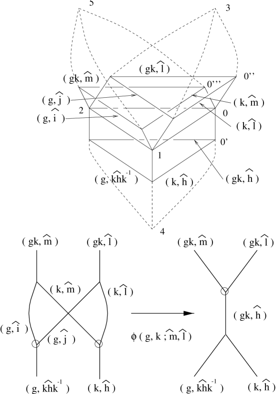
Figure 34: Weight for faces

6.1.5

Lemma. (1) For a tetrahedron or dual tetrahedron, there are colors satisfying the local rule at every face or dual face.

(2) There are colors on the edges and dual edges adjacent to a given face satisfying the local rules.

(3) Let $C$ be a color assigned to the oriented edges (or dual edges) of a tetrahedron (or dual tetrahedron). Let $C^{\prime}$ be a color assigned to the same tetrahedron (or dual tetrahedron) with orientations reversed on some of the edges. Then $C^{\prime}$ is uniquely determined. If the color $C$ is assigned to oriented edges and dual edges that are adjacent to a face, then the color $C^{\prime}$ is uniquely determined when some of the edges or dual edges have their orientations reversed.

Proof. We prove (1) and (2) in the case of tetrahedra. The proof for dual tetrahedra is similar and follows from [44].

For tetrahedra, the situation is depicted in Fig. 32. In the top of the figure, a tetrahedron with colors on three edges is depicted. Other edges receive compatible colors that are determined by these three. In the middle, pairs of front faces and back faces are depicted in the left and right respectively, together with dual graphs. In the bottom of the figure, only the dual graphs are depicted, together with colors on all the edges. We check that the first factors of colors match in multiplication convention in Fig. 31. The second factors are also checked as follows: in the bottom left figure, $\ell=mnm^{-1}$ and $h=k\ell k^{-1}$. In the bottom right figure, $\ell=mnm^{-1}$ (the same relation as above) and $h=((km)n(km)^{-1})$ which reduces to $kmnm^{-1}k^{-1}=k\ell k^{-1}$, the same relation as above. Thus the requirements on faces match at a tetrahedron.

To prove (3) for tetrahedra, first consider the case where the orientation of the edge $23$ is reversed. Then the face $(123)$ forces the change $S(-23|0123)=(g^{-1},\widehat{gk\ell k^{-1}g^{-1}})$. The other face $(023)$ forces the change $S(-23|0123)=(g^{-1},\widehat{(gkm)n(gkm)^{-1}})$. These are equal since $\ell=mnm^{-1}$. The situation is depicted in the top right of Fig. 33 where the reversed orientations are depicted by a small circle on the edge. The top left figure indicates the original colors. In the figure, the “hats” on the dual group elements are abbreviated for simplicity.

The other cases when the orientation of a single edge is reversed, are also depicted for the cases $(0213)$, $(1023)$. The general case follows because all cases are obtained by compositions of these changes.

Next consider statement (2). In Fig. 34 the colors are depicted using dual graphs (identify this graph with the graph in Fig. 25). First we check the orientation conventions in the figure. Identify the circled vertex of the right-hand-side graph of bottom of Fig. 25 with the right-hand-side of Fig. 31. Then the orientation conventions of dual edges coincide where $e_{1}$ of Fig. 31 corresponds to the edge $(02)\subset(0123)$, $e_{2}$ to $(02)\subset(0125)$, $e_{3}$ to $(02)\subset(0124)$. The tetrahedron $(0123)$ is shared by $(01234)$ and $(01235)$, that are ordered as $(01234)<(01235)<(01245)$ among three $4$-simplices. Thus this correspondence to $e_{1}$ matches with the definition of the orientation of dual edges.

Now we check the constraints. In the left bottom of Fig. 25 the following relations must hold: $i=kmk^{-1}$ (from the top left vertex), $j=k\ell k^{-1}$ (from the top right vertex), $h=m\ell$ (from the bottom right vertex), and $ij=khk^{-1}$ (from the bottom left vertex). The last relation is reduced by substitution to $k(m\ell)k^{-1}$ both sides, so that the weight is compatible. In the right of the figure, we get the relation $h=m\ell$ from the top vertex, which is the same as above, and the condition for the bottom vertex is already incorporated (by using $khk^{-1}$ in bottom left). Thus the colors around a face are compatible.

Now let us check that the orientation conventions are compatible in Fig. 34. The orientations on the edges are the orientations from the vertex ordering as seen in the figure. The orientations on dual edges are checked as follows. In the figure the face $(012)$ is shared by three $4$-simplices, $(01234)$, $(01245)$, and $(01235)$. The dual edge labeled by $(gk,\hat{\ell})$ is dual to the tetrahedron $(0123)$ and oriented from $(01234)$ to $(01235)$, corresponding to the edge $e_{1}$ on the right of Fig. 31. Respectively, the one labeled by $(gk,\hat{m})$ goes from $(01235)$ to $(01245)$ corresponding to $e_{2}$, the one labeled $(gk,\hat{h})$ goes from $(01234)$ to $(01245)$ corresponding to $e_{3}$. Thus the orientations defined from the order on vertices match the convention in Fig. 31.

To prove part (3), we check the cases of interchanging the orientation of some of the edges. The general case will follow from the cases depicted in Fig. 40 and 41 since the orientation changes depicted therein generate all the orientation changes.

First consider the case where the edge $(12)$ has reversed orientation. This corresponds to changing the vertex order from $(012345)$ in the figure to $(021345)$. (The orientations on dual edges do not change.) Then three colors change: $(g,\hat{i})$ to $(g^{-1},\widehat{(gk)m(gk)^{-1}})$, $(g,\hat{j})$ to $(g^{-1},\widehat{(gk)\ell(gk)^{-1}})$, and $(g,\widehat{khk^{-1}})$ to $(g^{-1},\widehat{(gk)h(gk)^{-1}})$. These changes are forced by the rules at faces (uncircled trivalent vertices of the graphs). Hence we check the rules at circled trivalent vertices. The only relevant vertex is the one on the left bottom in the figure. It must hold that $(gk)h(gk)^{-1}=(gk)m(gk)^{-1}\cdot(gk)\ell(gk)^{-1}$. This indeed follows from $h=m\ell$. The other cases are similar. $\Box$

6.1.6

Lemma. The colors define a function $\Psi^{\prime}:{\cal F}C\rightarrow G\times\hat{G}$ where $C$ is a perturbed carrier of $\Phi$ and ${\cal F}C$ is the set of $2$-faces of $S$. Conversely, a function $\Psi^{\prime}:{\cal F}C\rightarrow G\times\hat{G}$ defines a color $S$ defined for the triangulation $\Phi$ and $\Psi=\Phi\cup\Phi^{!}$.

Proof. This follows from Lemma 4.2.2 and the definition of $S$. $\Box$

6.2

Weighting. A weighting (also called a Boltzmann weight) is defined for each tetrahedron, face, edge of triangulations $\Phi$ and $\Phi^{!}$ as follows.

6.2.1

Definition (weights for tetrahedra). Let $T\in\Phi$ be a tetrahedron with vertices $0$, $1$, $2$, and $3$. Suppose $S(01|0123)=(m,\hat{n})$, $S(12|0123)=(k,\hat{l})$, and $S(23|0123)=(g,\hat{h})$.

The weight of $T$ with respect to the given labelings of edges is a number (an element of the ground field) defined by

$$B(T)=B(0123)=\alpha(g,k,m;\hat{n})^{\epsilon(T)}.$$

Here $\epsilon(T)$ is $\pm 1$ and is defined as follows. Let $T=(a_{0},a_{1},a_{2},a_{3})$ be the tetrahedron in consideration where $a_{0}<a_{1}<a_{2}<a_{3}$. Then $T$ is shared by two $4$-simplices, say, $S=(a_{0},a_{1},a_{2},a_{3},v)$ and $(a_{0},a_{1},a_{2},a_{3},w)$. Here we ignore the given labels of $v$ and $w$, and consider the orders written above ($v$ and $w$ coming last). Then exactly one of these two $4$-simplices, say, $S$, with this order $a_{0}<a_{1}<a_{2}<a_{3}<v$, matches the orientation of the $4$-manifold, and the other has the opposite orientation.

Consider the label on $v$ induced by the ordering on the vertices. If the integer index of $v$ is such that the oriented simplex $(a_{0},a_{1},a_{2},a_{3},v)$ is obtained from the order induced by labeling by an even permutation, then $\epsilon(T)=1$. Otherwise, $\epsilon(T)=-1$. (Sometimes we represent the order of vertices by labeling the vertices by integers.)

6.2.2

Definition (weights for faces). Suppose that a face $F=(012)$ is shared by three tetrahedra $(0123)$, $(0124)$, and $(0125)$. Suppose $S_{0}(01|0123)=(k,\hat{\ell})$, $S_{0}(12|0123)=(g,\widehat{k\ell k^{-1}})$, $S_{0}(02|0123)=(gk,\hat{\ell})$, $S_{0}(01|0124)=(k,\hat{h})$, and $S_{0}(02|0125)=(gk,\hat{m})$. The situation is depicted in Fig. 34.

Then the weight for the face $F=(012)$ is defined as the number

$$B(F)=B(012)=\phi(g,k;\hat{m},\hat{l})^{\epsilon(F)}.$$

Here the sign $\epsilon(F)=\pm 1$ is defined as follows. If the local orientation defined by $(012)$ in this order together with the orientation of the link $(34)\rightarrow(45)\rightarrow(53)$ of $F$ in this order gives the same orientation as that of the $4$-manifold, then $\epsilon(F)=1$, otherwise $\epsilon(F)=-1$.

Suppose the face $(012)$ is shared by $n$ (more than three) tetrahedra $(012k)$, $k=3,\cdots,n$. Note that the vertices of these tetrahedra other than $0,1,2$ form a link of the face $(012)$. Assume that these vertices are cyclically ordered by $3,4,\cdots n$, and that the link of $(012)$ and $(34)\rightarrow(45)\rightarrow\cdots\rightarrow(n3)$ matches the orientation of the $4$-manifold. Suppose $S(01|0124)=(k,\hat{\ell})$, $S_{0}(12|0124)=(g,\widehat{k\ell k^{-1}})$, $S_{0}(02|0124)=(gk,\hat{\ell})$, $S_{0}(01|0125)=(k,\widehat{m_{1}})$, $S_{0}(01|012k)=(k,\widehat{m_{k-4}})$, ($k=5,\cdots,n-1$), $S_{0}(01|012n)=(k,\widehat{m_{n-4}^{-1}})$. Then

$B(F)=B(012)=\phi(g,k;\widehat{m_{1}},\hat{\ell})\phi(g,k;\widehat{m_{2}},\widehat{m_{1}\ell})\cdots$

$\phi(g,k;\widehat{m_{n-5}},\widehat{m_{n-6}\cdots m_{1}\ell})\phi(g,k;\widehat{m_{n-4}},\widehat{m_{n-5}\cdots m_{1}\ell}).$

If the cyclic order of vertices is not as above, then it can be obtained from the above by transpositions. When a transposition between $k$-th and $(k+1)$-st vertex occurs, change the argument of $k$-th weight $\phi(g,k;\widehat{m_{k}},\widehat{m_{k-1}\cdots m_{1}\ell})$ to $\phi(g,k;\widehat{m_{k}^{-1}},\widehat{m_{k-1}\cdots m_{1}\ell})$.

Notice that by the conditions in the definition of a triangulation each face must be shared by at least three tetrahedra. However In the course of computation we may have to deal with singular triangulations. In this case it can happen that only two tetrahedra share a face. Let $0123$ and $0124$ be such two terahedra sharing the face $012$. Then the weight assigned to the face $012$ in this case is the product of Kronecker’s deltas:

$$\delta_{S(01|0123),S(01|0124)}\delta_{S(02|0123),S(02|0124)}\delta_{S(12|0123),S(12|0124)}$$

There are other cases of singular triangulations that appear in our proofs of well-definedness, and their weights are defined as follows.

Suppose that two tetrahedra share vertices $0,1,2,3$ and share all of their faces except $(013)$. Meanwhile, suppose that the face $(013)$ on each of the respective tetrahedra is shared with tetrahedra $(0134)$ and $(0135)$. The other faces are shared by the tetrahedra $(0126)$, $(0237)$, and $(1238)$. The situation is depicted in Fig. 42 top. In the figure, colors and weights are also depicted. The signs for each weight $\phi$ are also depicted in the figure in this situation, by indicating the power $-1$ on one of the $\phi\/$s.

Suppose in another situation that two tetrahedra share all vertices and all $2$-faces (triangles) as depicted in Fig. 43. The signs for this situation are also depicted in the figure.

In general if the order of vertices are different, then they are obtained from the above specific situations by compositions of permutations. Then the weights and signs are defined by applying Lemma 6.1.5.

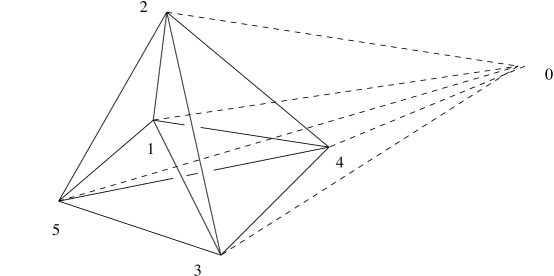
Figure 35: A triangulation of the 4-ball

6.2.3

Definition (weights for edges). Consider the triangulation of the 3-sphere $S^{3}$ consisting of 5 tetrahedra $(1234)$, $(1235)$, $(1245)$, $(1345)$, and $(2345)$, where integers represent the vertices. This triangulation is depicted in Figure 35 by solid lines. Here, the subdivided tetrahedron with vertices $2,3,4$ and $5$ with the interior vertex $1$ is a triangulation of a 3-ball, and together with the “outside” tetrahedron $(2345)$ they form a triangulation of $S^{3}$. Now take a cone of this triangulation with respect to the vertex $0$ to obtain a triangulation of a $4$-ball consisiting of 5 $4$-simplices $(01234)$, $(01235)$, $(01245)$, $(01345)$, and $(02345)$. This is depicted in Figure 35 also, where edges having $0$ as end point are depicted by dotted lines. (Regard dotted lines as lying in the interior of the $4$-ball.)

Suppose an edge $E=(01)$ has this particular triangulation as the neighborhood. Suppose $S(01|0123)=(g,\hat{\ell})$, $S(01|0124)=(g,\hat{k})$, and $S(01|0125)=(g,\hat{j})$. Then the weight for the edge $(01)$ is defined by

$$B(E)=B(01)=\beta(g;\hat{j},\hat{k},\hat{\ell})^{\epsilon(E)}.$$

The sign $\epsilon(E)=\pm 1$ is defined in the same manner as $B(T)$ simply taking the dual orientations.

If the neighborhood of an edge has a different triangulation, then the weight is defined as follows. Let $H_{1},\cdots,H_{s}\in\Phi^{!}$ be the set of tetrahedra of the polytope $p\in\Phi^{*}$, and let $h_{i}^{j}$ be the set of edges of $H_{i}$, $j=1,\cdots,6$. Then the weight is defined by

$$B(E)=1/|G|^{2a}\sum\prod\beta(g;\widehat{j_{f}},\widehat{k_{f}},\widehat{\ell_{f}})$$

where each $\beta$ is assigned to a tetrahedron of the above triangulation following the order convention of vertices. The product of the above expression is taken over all the shared edges, and the sum is taken over all the possible states on shared edges. The exponent, $a$, on the normalization factor, $1/|G|^{2a}$, is the number of verticies in the interior of the polyhedron dual to the given edge.

Figure 36: Movies of cocycle trees, Part I

Figure 37: Movies of cocycle trees, Part II

6.3

Partition function. Let $\Phi$ be a triangulation of a $4$-manifold $M$ with the set of vertices (resp. edges, faces, tetrahedra) ${\cal V}$ (resp. ${\cal E}$, ${\cal F}$, ${\cal T}$). Fix also a triangulation $\Phi^{!}$ of the dual $\Phi^{*}$.

6.3.1

Definition. The partition function $\psi(\Psi)$ for a triangulation $\Psi=\Phi\cup\Phi^{!}$ with a total order on vertices is defined by

$$\psi(\Psi)=1/|G|^{2a}\sum_{S}\prod_{{\cal T},{\cal F},{\cal E}}B(T)B(F)B(E)$$

where the product ranges over tetrahedra, faces and edges of the triangulation $\Phi$, the summation ranges over all the possible states, and the exponent $a$ on the normalization factor is the number of vertices in the triangulation.

6.3.2

Main Theorem. The partition function $\psi(\Psi)$ defined above for triangulations $\Psi=\Phi\cup\Phi^{!}$ of a 4-manifold $M$ is independent of the choice of the triangulation $\Phi$ and $\Phi^{!}$ and independent of choice of order on vertices.

Therefore the partition function $\psi$ defines an invariant of a 4-manifold $M$.

Section 7 is devoted to giving the proof of this theorem.

6.4

Diagrams, cocycles, and triangulations. Here we explain relations among diagrams, cocycles, and triangulations. Figure 31 illustrates the coloring rules at triangles and dual triangles. In these triangles and dual triangles graphs are embedded; the verticies of the graphs in the dual triangles are labeled by small circles. The cocycles $\alpha$ are assigned to tetrahedra; the cocycles $\beta$ are assigned to dual tetrahedra, and the cocycles $\phi$ are assigned to triangular faces. Each such figure also corresponds to a graph movie which depicts a part of the perturbed carrier surface. We can think of the cocycles as being assigned to the vertices of the perturbed carrier surface which has a tripartition on its vertex set. Indeed the many scenes that constitute the graph movie are found on the boundary of a regular neighborhood of the vertices of the carrier surface. In this way we can directly visualize the construction of the invariant as a colored surface with weighted vertices or as a colored graph movie with weights associated to the scenes.

Simliarly, the cocycle conditions can be described as relations on movies of tree diagrams. Figures 36 and 37 depict these relations. Each change of a tree diagram (scene in the movie) corresponds to a cocycle as indicated. When we multiply the left-hand-side and the right-hand-side of cocycles in the movies, we obtain cocycle conditions among $\alpha$, $\phi$, and $\beta$.

The cocycle conditions can also be understood in terms of certain singular surfaces that are embedded in the 4-manifold. These surfaces are depicted in Figs. 38 and 39. In these figures the cocycles $\phi$ corresponds to the surface $(Y\times Y)$ and the cocycle $\alpha$ corresponds to the surface that is dual to a tetrahedron. The assignment of $\phi$ to $Y\times Y$ is indicated in the weights on Fig. 26. The reasons for these assignments is that the cocycle $\phi$ is found when three tetrahedra share a triangular face, and the cocycle $\alpha$ is assigned to a tetrahedra. In Figs. 38 and 39 some edges are denoted as tubes. A tube of the form $\circ\times Y$ corresponds to a triangle that is shared by three tetrahdra as in Fig. 25.

Figure 38: Surface of cocycle movies: left hand side

Figure 39: Surface of cocycle movies: right hand side

7 On invariance of the partition function

Recall the notation in Section 6: $\Phi$ denotes a triangulation of a 4-manifold $M$, $\Phi^{*}$ its dual complex, $\Phi^{!}$ a 3-face triangulation of $\Phi^{*}$. In Section 7.1 we show that the partition function defined is independent of the order on vertices. In Section 7.2, we show that the partition function is independent of the triangulation. In Section 7.3 we show that the partition function is independent of the choice of dual triangulation.

Figure 40: Symmetries of $\phi$, Part I

Figure 41: Symmetries of $\phi$, Part II

7.1

Independence on order of vertices. In this section we prove

7.1.1

Lemma. The cocycle symmetries imply the independence of the partition function on the order on vertices of the triangulation.

Proof. For tetrahedra and dual tetrahedra, the weights are the cocycles $\alpha$ and $\beta$ respectively. As in [44], it is sufficient to check how weights change when the order of vertices are changed from $(0123)$ to $(0132)$, $(0213)$, and $(1023)$. Such changes are illustated in Fig. 33 for $\alpha$, and the corresponding conditions are listed for $\alpha$, $\beta$ and $\phi$ in Section 5.2.1.

For a face, we check as follows. In Fig. 34 an order of vertices are given, where the face is given by $(012)$, and the other vertices are given labels $3$, $4$, and $5$. The changes of orders of vertices are generated by the changes from $(012345)$ to $(021345)$, $(102345)$, (for the face) $(012354)$, $(012435)$, (for the dual face) since only the relative orders among the vertices of the face and those of the dual faces are in consideration. For these changes, the colors are listed in Fig. 40 and Fig. 41. They are depicted in terms of dual graphs, and on the right hand side, the orientations of edges of faces/dual faces are shown. The small circles indicate reversed orientations. The corresponding conditions are listed in Section 5.2.1.

If more than three tetrahedra share a face, then a change in order of the vertices can be achieved by such pairwise switches. Futhermore, in order to affect such changes, we may have to group the vertices in sets of 3. This grouping is achieved by a 3-face triangulation. So the proof will follow once we have shown invariance under the 3-face triangulation. $\Box$

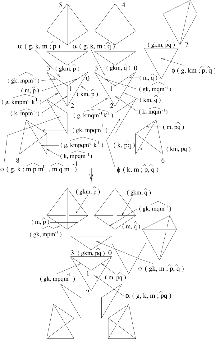
Figure 42: Colors and cocycles for the cone move

7.2

Independence under Pachner moves. In this section, we explicitly relate the cone move, taco move and pillow move to the cocycle conditions. Since these moves and lower dimensional moves generate the Pachner moves, we will use the cocycle conditions to show that the partition function is invariant under the Pachner moves.

7.2.1

Lemma. The partition function is invariant under the cone move for a local triangulation with a specific choice of order depicted in Fig. 42.

Proof. Let $(0123)_{1}$ and $(0123)_{2}$ be tetrahedra sharing the same faces $(012)$, $(013)$ and $(023)$, but having different faces $(123)_{1}$ and $(123)_{2}$, such that (1) the union of the triangles $(123)_{1}$ $\cup$ $(123)_{2}$ bounds a 3-ball $B$ in the 4-manifold, (2) the union of $B$ , $(0123)_{1}$ and $(0123)_{2}$ is diffeomorphic to the $3$-sphere bounding a $4$-ball $W$ in the 4-manifold. (See Figs. 15, 42.) In these figures, the movies of dual graphs are depicted where each of the faces $(013)$, $(023)$, $(123)$ is shared by another tetrahedron ($(0124)$, $(0125)$, $(0126)$, respectively). We prove the invariance in this case. The general case follows from such computations together with the pentagon identity of $\beta$.

Fig. 42 shows the colors and cocycles assigned to this local triangulation (again note the direct relation between this assignment and those for the top graph in Fig. 36). The left hand side of the cone move (top of Fig. 42) has the local contribution

$$\phi(g,km;\hat{p},\hat{q})\phi(k,m;\hat{p},\hat{q})\phi(g,k;\widehat{mpm^{-1}},\widehat{mqm^{-1}})^{-1}\alpha(g,k,m;\hat{p})\alpha(g,k,m;\hat{q}),$$

(note that the orientation of the face $(9123)$ is opposite), and the right hand side of the cone move (bottom of the figure) has the local contribution

$$\phi(gk,m;\hat{p},\hat{q})\alpha(g,k,m;\widehat{pq}).$$

Thus the partition function is invariant under the cone move because the cocycle condition is satisfied. $\Box$

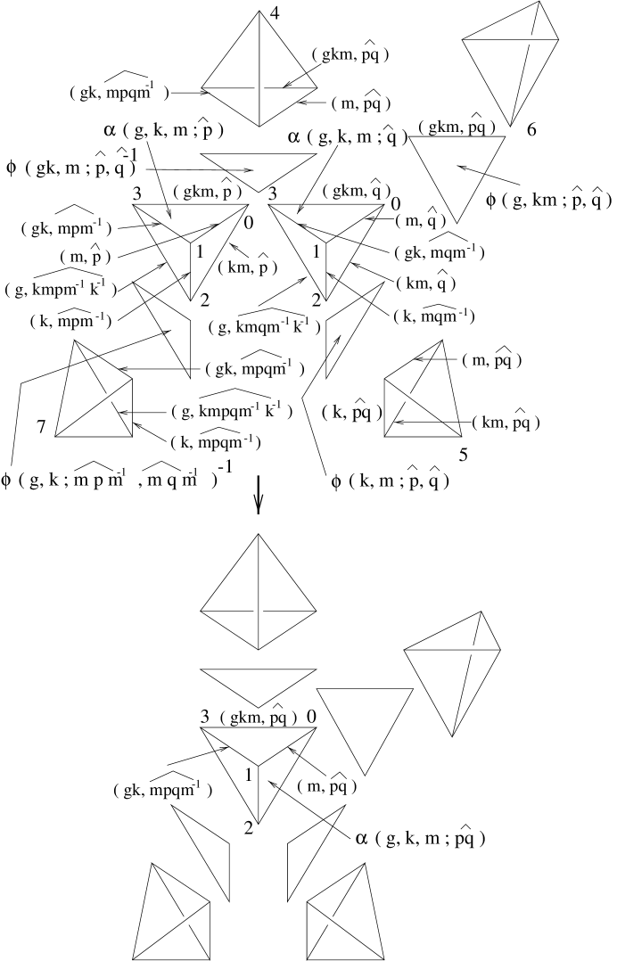
Figure 43: Colors and cocycles for the pillow move

Figure 44: Colors and cocycles for the taco move

7.2.2

Lemma. The partition function is independent under the pillow move for a specific local triangulation with the order depicted in Fig. 43.

Proof. In Fig. 43 the assignments of colors and cocycles are shown. The left hand side of the pillow move (top of Fig. 43) has the local contribution

$$\phi(g,km;\hat{p},\hat{q})\phi(k,m;\hat{p},\hat{q})\phi(gk,m;\hat{p},\hat{q})^{-1}\phi(g,k;\widehat{mpm^{-1}},\widehat{mqm^{-1}})^{-1}\alpha(g,k,m;\hat{p})\alpha(g,k,m;\hat{q}),$$

and the right hand side of the pillow move (bottom of the figure) has the local contribution $\alpha(g,k,m;\widehat{pq}).$ This follows from the cocycle condition used in the above lemma. $\Box$

7.2.3

Lemma. The partition function is independent under the taco move for a specific local triangulation with the order depicted in Fig. 44.

Proof. In Fig. 44 the assignments of colors and cocycles are shown. The left hand side of the taco move (top of Fig. 44) has the local contribution

$$\phi(g,km;\hat{p},\hat{q})\phi(k,m;\hat{p},\hat{q})\alpha(g,k,m;\hat{p})\alpha(g,k,m;\hat{q}),$$

and the right hand side of the taco move (bottom of the figure) has the local contribution

$$\phi(gk,m;\hat{p},\hat{q})\phi(g,k;\widehat{mpm^{-1}},\widehat{mqm^{-1}})\alpha(g,k,m;\widehat{pq}).$$

This is exactly one of the cocycle conditions. $\Box$

Observe that the diagrammatics of the graph movie move that results from the taco move match exactly the graph movie move that represents the cocycle condition Fig. 36. Similar graph movies can be drawn for the cone and pillow moves and the correspondence with the move and the coycle conditions can be worked out via the graph movies. Making such correspondence shows explicitly the method of constructing invariants via Hopf categories where, instead of cocycle conditions, coherence relations are used. The coherence relations can be expressed by such graph movie moves (See Section 8).

Since the partition function is invariant under the cone, taco, and pillow moves, and since $\alpha$ satisfies a pentagon relation, we have the partition function is invariant under the Pachner moves.

7.3

Independence on triangulations of the dual complexes. In this section, we complete the proof that the partition function is well-defined by showing that the partition function does not depend on the 3-face triangulation, $\Phi^{!}$.

7.3.1

Lemma. If $T_{1}$ and $T_{2}$ are triangulations of a $3$-dimensional polytope which is diffeomorphic to a $3$-ball such that $T_{1}$ and $T_{2}$ restrict to the same triangulation on the boundary, then they are related by a finite sequence of Pachner moves.

Proof. We first prove the corresponding statement in dimension 2, then use the result in dimension 2 to achieve the result in dimension 3. In the proof we use the notation $(i\rightleftharpoons j)$-move to indicate the move in which $i$ simplices are replaced by $j$ simplices. So the $(j\rightleftharpoons i)$-move is the inverse move, and the order of $i$ and $j$ matter.

In dimension 2, we have two triangulations of the disk that agree on the boundary, and we are to show that they they can be arranged by Pachner moves fixing the boundary to agree on the interior. We prove the result by induction on the number of vertices

on the boundary.

Recall [39] [7], that the star of a $k$-simplex (in a simplicial complex) is the union of all the simplices that contain the $k$-simplex. The link of a $k$-simplex is the union of all the simplices in the star that do not contain the $k$-simplex. We will examine the stars and links of vertices on the boundary of a disk (and later on the bounday of a 3-ball). So denote the

star of $v$ with respect to the boundary by: ${\mbox{\rm st}}_{S}(v)$. Similarly, the link of $v$ with respect to the boundary is ${\mbox{\rm lk}}_{S}(v)$ while these sets with respect to the interior are ${\mbox{\rm st}}_{B}(v)$ and ${\mbox{\rm lk}}_{B}(v)$, respectively.

In dimension 2, ${\mbox{\rm st}}_{S}(v)$ is a pair of edges that share the vertex $v$. Meanwhile, ${\mbox{\rm lk}}_{B}(v)$ is a polygonal path properly embedded in the disk that is the most proximate to $v$ among all paths in the interior that join the points of ${\mbox{\rm lk}}_{S}(v)$.

We fix our consideration on one of the triangulations, say $T_{1}$ of $D^{2}$. We want to alter this triangulation so that ${\mbox{\rm lk}}_{B}(v)$ is an edge (so it has no interior vertices). If we can achieve this alteration, then we can perform similar moves to $T_{2}$. The vertex $v$ on either triangulation then will become the vertex of a triangle that is attached to the disk along a single edge.

We can remove such a triangle (or alternatively, work in the interior) and apply induction on the number of vertices on the boundary.

Consider an interior vertex, $v^{\prime}$ in $B$. If the star of $v^{\prime}$ in $B$ is the union of three triangles at $v^{\prime}$, then we can remove this vertex from $D$ by means of a $(3\rightleftharpoons 1)$-move. Perform such moves until there are no interior vertices of valence 3. In this way we may assume that a vertex, $v^{\prime\prime}\in{\mbox{\rm lk}}_{B}(v)$ has valence larger than 3. If the valence of $v^{\prime\prime}$ is greater than $3$, then there are a pair of triangles in ${\mbox{\rm st}}_{B}(v)$ sharing edge $v,v^{\prime\prime}$ upon which a Pachner move of type $(2\rightleftharpoons 2)$ can be performed. Such a move removes $v^{\prime\prime}$ from the link of $v$. After such a move, check for interior vertices of valence 3 and remove them by type $(3\rightleftharpoons 1)$-moves. In this way we can continue until the link of $v$ is an edge. If $D$ is a triangle, then the process will reduce the triangulation until there are no interior vertices.

Now we mimic the proof given in dimension 2, to dimension 3. First, assume that an interior vertex $v^{\prime}$ in $D^{3}$ has as its star the union of 4 tetrahedra. Then we may eliminate such an interior vertex by means of a type $(4\rightleftharpoons 1)$ Pachner move.

Consider the link, ${\mbox{\rm lk}}_{B}(v)$ of a vertex, $v$, on the boundary. If this link is a triangle, then we may eliminate the vertex from the boundary, as in the 2-dimensional case. For the star of $v$ is a single tetrahedron that is glued to the ball along a single face.

More generally, ${\mbox{\rm st}}_{S}(v)$ is a union of triangles forming a polygon, so ${\mbox{\rm st}}_{S}(v)$ is the cone on the polygon ${\mbox{\rm lk}}_{S}(v)$ where $v$ is the cone point. Consider the disk properly embedded in $B$ that is the link of $v$. This link, ${\mbox{\rm lk}}_{B}(v)$, is a triangulated disk. There is a sequence of 2-dimensional Pachner moves that change ${\mbox{\rm lk}}_{B}(v)$ to a triangulation of an $n$-gon, with no interior vertices. We use these 2-dimensional moves to determine $3$-dimensional moves performed in a neighborhood of ${\mbox{\rm st}}_{B}(v)$ as follows.

Suppose that a $(3\rightleftharpoons 1)$-move is used to simplify the disk that is the link of $v$. Then consider the vertex $v^{\prime}$ at which such a move is performed. By our first step, its star is not the union of 4 tetrahedra. Three tetrahedra intersect along the edge, $v,v^{\prime}$, and a $(3\rightleftharpoons 2)$-move can be performed in the star of $v$ to remove the vertex $v^{\prime}$ from the link. After such a move, then check for vertices in the interior whose valence is $4$. Remove these by $(4\rightleftharpoons 1)$-moves, until no such vertices remain. Potentially, some vertices from the link of $v$ are removed, and the effect of such a removal on the link is to perform a $(3\rightleftharpoons 1)$-move. In general a $(3\rightleftharpoons 1)$-move to the link corresponds to a $(3\rightleftharpoons 2)$-move to the star, or a $(4\rightleftharpoons 1)$-move to a part of the star and a tetrahedron on the other side of the link.

If a $(2\rightleftharpoons 2)$-move is used to simplify ${\mbox{\rm lk}}_{B}(v)$, then there is either a $(3\rightleftharpoons 2)$-move or a $(2\rightleftharpoons 3)$-move to that ball which induces it. Specifcally, if an edge in ${\mbox{\rm lk}}_{B}(v)$ has as its star the union of 3 tetrahedra, then two of these are found in ${\mbox{\rm st}}_{B}(v)$ and the other one is on the other side of the link of $v$. In this case perform a $(3\rightleftharpoons 2)$-move to $B$. The link of $v$ changes by a $(2\rightleftharpoons 2)$-move. If the link of the edge to be changed is more than 3 tetrahedra, then perform a $(2\rightleftharpoons 3)$-move to ${\mbox{\rm st}}_{B}(v)$. In this way, a triangulation always results from these moves. After each such move, one must go and check for vertices of valence $4$ and remove them by $(4\rightleftharpoons 1)$-moves.

Eventually, we can remove all interior vertices from ${\mbox{\rm lk}}_{B}(v)$ and we can further make sure that the link of $v$ is in some standard position. We can remove $v$ from the boundary of $B$ by removing $v$ and the $(n-2)$-tetrahedra in its star where $n$ is the valence of $v$ with repsect to the boundary. The result follows by induction. $\Box$

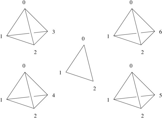
Figure 45: A face sharing four tetrahedra

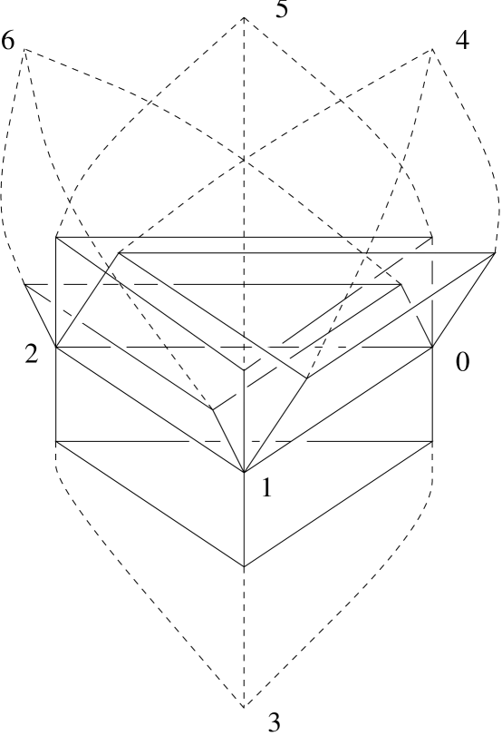
Figure 46: A face sharing four tetrahedra, another view

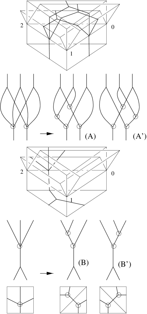
Figure 47: Dual graphs around a face sharing four tetrahedra

7.3.2

Lemma. The partition function $\psi$ does not depend on the choice of $3$-face triangulations of $\Phi^{*}$.

Proof. First let us analyze the case when a face $(012)$ is shared by four tetrahedra. Then we will discuss the general case. Figures 45 and 46 depict the case where a face $(012)$ is shared by four tetrahedra $(0123)$, $(0124)$, $(0125)$ and $(0126)$.

Then the dual complex has a rectangular $2$-face $(012)^{*}$ which is dual to the face $(012)$. There are two triangulations of a rectangle, say $t_{1}$ and $t_{2}$, for $(012)^{*}$. (These are the triangulations that have no interior vertices). The $3$-polytopes in $\Phi^{*}$ that share $(012)^{*}$ are duals $(01)^{*}$, $(02)^{*}$ and $(12)^{*}$. Let $T_{1}$ and $T_{2}$ be $3$-face triangulations of $\Phi^{*}$ that restrict to $t_{1}$ and $t_{2}$ respectively and restrict to the same triangulation on all the other $2$-faces of $\Phi^{*}$. We show that the partition functions defined from $T_{1}$ and $T_{2}$ give the same value.

Recall (Fig. 6) that two pairs of faces of a tetrahedron give two triangulation of a rectangle. We attach a tetrahedron in between $(012)^{*}$ and $(01)^{*}$ and change the triangulations on the face. More specifically, attach a pair of adjacent faces of a tetrahedron onto the face $(012)^{*}$ of $(01)^{*}$ along the triangulation $T_{1}$ restricted to $t_{1}$. Perform the same attachment for $(02)^{*}$ and $(12)^{*}$. Then we get a new triangulation $T_{1}^{\prime}$ of $\Phi^{*}$ which restricts to $t_{2}$ on $(012)^{*}$. Thus $T_{1}^{\prime}$ and $T_{2}$ have the same triangulation on the $2$-skeleton of $\Phi^{*}$ by the assumption that all the other faces have the same triangulation. Thus $T_{1}^{\prime}$ and $T_{2}$ are related by a finite sequence of Pachner moves fixing the boundary triagulation by Lemma 7.3.1 which does not change the partition function by the pentagon identity and the orthogonality of the cocycle $\beta$. Hence it remains to prove that $T_{1}$ and $T_{1}^{\prime}$ give the same value of the partition function.

If the dual face $(012)^{*}$ is in general a polygon of more than four faces (say $n$-gon), then triangulations consist of $(n-2)$ triangles (by the condition of the definition of $3$-face triangulation). Such trianglations are related by only $(2\rightleftharpoons 2)$-moves, which are realized by attaching a pair of faces of tetrahedra once at a time as above. Thus the above argument is applied to general cases by repeating the argument.

Now we prove that $T_{1}$ and $T_{1}^{\prime}$ in the case $(012)^{*}$ is a rectangle give the same value of the partition function. Figure 47 depicts the graphs for the triangulation. In Fig. 47 the perturbations of these graphs to trivalent graphs are also depicted. These perturbations correspond to $\Psi^{!}$ (triangulations of a rectangle $(012)^{*}$ in this case) as depicted in the bottom of Fig. 47. Thus the colors assigned near the face $(012)$ with triangulations $T_{1}$ and $T_{1}^{\prime}$ are also assigned to edges of the perturbed graphs (the right pictures of arrows in the figure, marked (A), (A’), (B), and (B’)).

These graphs are identified by the following graphs in Fig. 37: (A) corresponds to top graph, (A’) to top left, (B) to bottom right, (B’) to bottom. The weights $\phi$ assigned to each triangulation are thus $\phi(g,k;\hat{p},\hat{r})\phi(g,k;\widehat{pr},\hat{s})$ for $T_{1}$ and $\phi(g,k;\hat{r},\hat{s})\phi(g,k;\hat{p},\widehat{rs},)$ for $T_{1}^{\prime}$ (or vice versa), if the group elements assigned are as indicated in Fig. 37.

Now since $T_{1}^{\prime}$ is obtained from $T_{1}$ by attaching three tetrahedra, and they receive the weights $\beta(g;\widehat{kpk^{-1}},\widehat{krk^{-1}},\widehat{ksk^{-1}})$, $\beta(k;\hat{p},\hat{r},\hat{s})$, $\beta(gk;\hat{p},\hat{r},\hat{s})$, therefore the cocycle condition depicted in Fig. 37 shows that they are equal. $\Box$

8 Hopf categories

8.1

Overview of Hopf categories. We refer the reader to [13, 17, 35] for details about Hopf categories. Here we give a brief overview. A Hopf category is a categorification of a Hopf algebra. Roughly speaking, this means that the multiplication between elements becomes the tensor product between two objects, and there is a cotensor product defined for objects.

First we recall $2$-categories from [29, 23, 6].

Figure 48: Compositions of $2$-morphisms

Figure 49: Horizontal composition

Figure 50: Unambiguous composition

8.1.1

Review of 2-categories.A (small) strict $2$-category consists of the following data:

(1) a set of objects Obj,

(2) a set of $1$-morphisms $1$-Mor, whose elements have source and target objects,

(3) a set of $2$-morphisms $2$-Mor, whose elements have source and target $1$-morphisms. Explicitly, given any two objects $A,B$, there is a set of $1$-morphisms $1$-Mor$(A,B)$ between them; the object $A$ is called the source object, $B$ is the target. Such a $1$-morphism $f$ is also denoted by $f:A\rightarrow B$. Given any two 1-morphisms $f$, $g\in$ $1$-Mor$(A,B)$ there is a set of 2-morphisms between them; $f$ is the source arrow ($1$-morphism), and $g$ is the target arrow ($1$-morphism). The object $A$ is the source object and the object $B$ is the target object (of the $2$-morphism). Therefore both the sources and targets of $f$ and $g$ are required to coincide. Such a $2$-morphism is also denoted by $\alpha:f\Rightarrow g$. (The smallness is the condition that these are sets.)

The following compositions of morphisms are defined and related as indicated in items (1) through (5).

(1) For any $1$-morphisms $f:A\rightarrow B$ and $g:B\rightarrow C$, a $1$-morphism $g\circ f(=gf):A\rightarrow C$ is the composite.

(2) For any $1$-morphism $f:A\rightarrow B$ and a $2$-morphism $\alpha:g\Rightarrow g^{\prime}$ between $1$-morphisms $g,g^{\prime}:B\rightarrow C$, there is a composition (a $2$-morphism) $\alpha f:gf\Rightarrow g^{\prime}f$. Similarly, there is a 2-morphism $g\alpha:gf\Rightarrow gf^{\prime}$ when $\alpha:f\Rightarrow f^{\prime}$. These compositions are depicted on the left and middle of Fig. 48.

(3) For any $2$-morphisms $\alpha:f\Rightarrow g$ and $\beta:g\Rightarrow h$ where $f,g,h:A\rightarrow B$, there is a composition $\beta\cdot\alpha:f\Rightarrow h$. This is depicted in Fig. 48 right. The composition $\beta\cdot\alpha$ is called the vertical composition of 2-morphisms.

(4) The composition depicted in Fig. 49 is unambiguous in the sense that

$$\beta\circ\alpha=(\beta f^{\prime})\cdot(g\alpha)=(g^{\prime}\alpha)\cdot(\beta f).$$

The result $\beta\circ\alpha$ is called the horizontal composition of the 2-morphisms $\alpha$ and $\beta$.

(5) The composition depicted in Fig. 50 is also unambiguous in the sense that

$$(\beta^{\prime}\cdot\beta)\circ(\alpha^{\prime}\cdot\alpha)=(\beta^{\prime}\circ\alpha^{\prime})\cdot(\beta\circ\alpha)$$

as 2-morphisms from $gf$ to $g^{\prime\prime}f^{\prime\prime}$.

We assume further that

$${\mbox{\rm id}}_{f}\circ\alpha=f\circ\alpha$$

and

$$\alpha\circ{\mbox{\rm id}}_{g}=\alpha g$$

where $f,g$ are 1-morphisms, $\alpha$ is a 2-morphism and these composites are defined.

For any object $A$ (resp. $1$-morphism $f$), the identity $1$-morphism ${\mbox{\rm id}}_{A}$ (resp. $2$-morphism ${\mbox{\rm id}}_{f}$) is defined. The identity $2$-morphism satisfies $({\mbox{\rm id}}_{f})\cdot\alpha=\alpha$ , $\alpha\cdot({\mbox{\rm id}}_{f})=\alpha$ for any $2$-morphism $\alpha$.

For any $2$-morphism $\alpha:f\Rightarrow g$ where $f,g:A\rightarrow B$ , $\alpha({\mbox{\rm id}}_{A})=\alpha$ and $({\mbox{\rm id}}_{B})\alpha=\alpha$.

The following are the conditions for the strictness.

(1) The compositions of $1$- and $2$-morphisms are associative ( $(fg)h=f(gh)$, $(\alpha\beta)\gamma=\alpha(\beta\gamma)$ ).

(2) For any $1$-morphism $f:A\rightarrow B$, $f({\mbox{\rm id}}_{A})=f=({\mbox{\rm id}}_{B})f$.

This concludes the definition of a small strict $2$-category.

Note that by composing morphisms we can represent $2$-morphisms by planar polygons. More on 2-categories can be found also in [11].

We follow the definitions in [35] for the rest of this section.

A monoidal $2$-category consists of a $2$-category ${\cal C}$ together with the data: (1) an object $I$, (2) for any object $A$ two $2$-functors ${\cal L}_{A}=A\mbox{ $\Box\raisebox{1.1pt}{$\times$}$}-:{\cal C}\rightarrow{\cal C}$ and ${\cal R}_{A}=-\mbox{ $\Box\raisebox{1.1pt}{$\times$}$}A:{\cal C}\rightarrow{\cal C}$ such that ${\cal L}_{A}(B)={\cal R}_{B}(A)$ for any objects $A$, $B$, and (3) for any two $1$-morphisms $f:A\rightarrow A^{\prime}$ and $g:B\rightarrow B^{\prime}$ a $2$-morphism

$$\mbox{ $\Box\raisebox{1.1pt}{$\times$}$}_{f,g}:(f\mbox{ $\Box\raisebox{1.1pt}{$\times$}$}B^{\prime})(A\mbox{ $\Box\raisebox{1.1pt}{$\times$}$}g)\Rightarrow(A^{\prime}\mbox{ $\Box\raisebox{1.1pt}{$\times$}$}g)(f\mbox{ $\Box\raisebox{1.1pt}{$\times$}$}B).$$

These data satisfy 8 conditions that we omit here.

A $2$-vector space is a $k$-linear additive category $({\cal C},\oplus)$ that admits a subset $B\subset{\cal C}$ such that (1) any object $X\in B$ is simple, (2) for any $X\in B$, $dim_{k}(Hom(X,X))=1$, and (3) for any object $A\in{\cal C}$ there is a unique finite subset $B^{\prime}\subset B$ such that $A\cong\oplus_{X_{i}\in B^{\prime}}X_{i}^{n_{1}}$. The set $B$ is called a basis and a $2-$vector space is finite if $B^{\prime}$ is finite.

The $2$-category of finite dimensional $2$-vector spaces is denoted by $2-vect$. The set of $1$-morphisms are $k$-linear functors, and $2$-morphisms are natural transformations. This is a subcategory of the $2$-category ${\cal C}_{k}$ of small $k$-linear additive categories with the $k$-linear functors as $1$-morphisms.

Theorem 2.7 of [35] says that $2-vect$ admits the structure of a strongly involutory moniodal 2-category in such a way that for ${\cal C},{\cal D}\in 2-$vect, Obj$({\cal C}\mbox{ $\Box\raisebox{1.1pt}{$\times$}$}{\cal D})=\{(A_{1},\cdots,A_{n})|A_{i}$ are pairs of objects of ${\cal C}$ and ${\cal D}$, Mor$((A_{1},\cdots,A_{n}),(B_{1},\cdots,B_{m}))=\{(f_{ij})|f_{ij}:A_{j}\Rightarrow B_{i}\}$.

A comoidal category is a category ${\cal C}$ in ${\cal C}_{k}$ with the following data. Two $k$-linear functors $\diamondsuit:{\cal C}\rightarrow{\cal C}\mbox{ $\Box\raisebox{1.1pt}{$\times$}$}{\cal C}$ and $\Gamma:{\cal C}\rightarrow{\mbox{\rm vec}}$ where vec=the category of vector spaces, and some natural isomorphisms, including $\alpha:(1\mbox{ $\Box\raisebox{1.1pt}{$\times$}$}\diamondsuit)\circ\diamondsuit\Rightarrow(\diamondsuit\mbox{ $\Box\raisebox{1.1pt}{$\times$}$}1)\circ\diamondsuit$, satisfying certain relations, including the pentagon relation for $\alpha$.

A $2$-bialgebra or a bimonoidal category is a category ${\cal C}\in{\cal C}_{k}$ which has both monoidal and comoidal category structures and with additional data including a natural isomorphism $\Xi:(\otimes\mbox{ $\Box\raisebox{1.1pt}{$\times$}$}\otimes)(1\mbox{ $\Box\raisebox{1.1pt}{$\times$}$}{\cal T}\mbox{ $\Box\raisebox{1.1pt}{$\times$}$}1)(\diamondsuit\mbox{ $\Box\raisebox{1.1pt}{$\times$}$}\diamondsuit)\Rightarrow\diamondsuit\otimes$ satisfying certain conditions, where ${\cal T}$ denotes permutations, including figures depicted in 52, 54, and 56. The faces in the figures are $2$-morphisms, and these cubes are relations among $2$-morphisms in the Hopf category.

8.2

Cocycle conditions and Hopf categories. The cocycles and their equations given in the previous sections to construct partition functions are given by Crane and Yetter [17] to construct examples of Hopf categories. We refer the reader to [17] and [35] for the detailed relation between cocycles and Hopf categories.

Here we give a sketch description. The Hopf category constructed is a categorification of the Drinfeld quantum double of a finite group. Thus first we recall $D(G)$, the quantum double of a finite group $G$. It is an algebra generated by pairs of gropus and dual group elements, $\{(g,\hat{h})\}$. The multiplication is defined by $(g,\hat{h})\cdot(k,\hat{\ell})=\delta_{k^{-1}hk,\ell}(gk,\hat{\ell})$, comultiplication by $\Delta((g,\hat{h}))=\sum_{k}(g,\hat{k})\otimes(g,\widehat{hk^{-1}})$. The unit is $I=\sum_{h}(g,\hat{h})$, the counit is $\Gamma(g,\hat{h})=\delta_{h,e}$, the antipode is $S(g,\hat{h})=(g^{-1},\widehat{gh^{-1}g^{-1}})$.

The Hopf category ${\cal C}={\cal D}(G)$, a categorification of $D(G)$, has the one dimensional vector space over a field $k$ generated by pairs $\{(g,\hat{h})\}$ as objects. They are also simply denoted by pairs. The functor ${\cal C}\mbox{ $\Box\raisebox{1.1pt}{$\times$}$}{\cal C}\rightarrow{\cal C}$ is a family of isomorphisms $(g,\hat{h})\otimes(k,\hat{\ell})\rightarrow(gk,\hat{\ell})$ where $h=k\ell k^{-1}$, and the functor $\diamondsuit:{\cal C}\rightarrow{\cal C}\mbox{ $\Box\raisebox{1.1pt}{$\times$}$}{\cal C}$ is given by a family $(g,\hat{h})\rightarrow\sum_{k}(g,\hat{k})\mbox{ $\Box\raisebox{1.1pt}{$\times$}$}(g,\widehat{xk^{-1}})$.

The transformation ($2$-morphism)

$$\alpha_{(g,\hat{h}),(k,\hat{\ell}),(m,\hat{n})}:((g,\hat{h})\mbox{ $\Box\raisebox{1.1pt}{$\times$}$}(k,\hat{\ell}))\mbox{ $\Box\raisebox{1.1pt}{$\times$}$}(m,\hat{n})\rightarrow(g,\hat{h})\mbox{ $\Box\raisebox{1.1pt}{$\times$}$}((k,\hat{\ell})\mbox{ $\Box\raisebox{1.1pt}{$\times$}$}(m,\hat{n}))$$

is a family of scalars $\alpha(g,k,m;\hat{n})$ since the objects are nontrivial only when $\ell=k^{-1}hk$ and $n=\ell^{-1}m\ell$. Similar for $\beta(g;\hat{i},\hat{j},\hat{k})$, and for the transformation $\Xi$, one has scalars

$$\phi(g,k;\hat{m},\hat{n}):\oplus_{mn=\ell}(gk,\hat{m})\mbox{ $\Box\raisebox{1.1pt}{$\times$}$}(gk,\hat{n})\rightarrow\oplus_{ab=h}(gk,\widehat{k^{-1}ak})\mbox{ $\Box\raisebox{1.1pt}{$\times$}$}(gk,\widehat{k^{-1}bk}).$$

Thus we get these cocycles as transformations (or $2$-morphisms) in a Hopf category. The cocycle conditions are obtained from the axioms of the Hopf categories.

Figure 51: Diagrams for morphisms

8.3

Diagrams for morphisms. We use the diagrammatic convention depicted in Fig. 51. The top two figures represent tensor and cotensor functors ($1$-morphisms). We read the diagram from bottom to top, the segments correspond to categories, and trivalent vertices correspond to tensor (uncircled vertices) functors and cotensor (circles ones) functors. Thus a tree diagrams represent compositions of such functors. The bottom three figures represent $2$-morphisms. For each of these, two compositions of functors are related by a double arrow representing a transformation ($2$-morphism) between $1$-morphisms that are compositions of tensor and cotensor functors.

For the categorification of the quantum double, the objects are represented by pairs $\{(g,\hat{h})\}$, therefore the edges of the graphs are labled by these pairs. The situation is seen in Fig. 31. The functors, then, are represented by trivalent vertices of the graphs. These are depicted in Figs. 32, 34. In Fig. 32, the functor corresponding to $\alpha$ is depicted, and in Fig. 34, the functor corresponding to $\phi$ (or $\Xi$) is depicted. The diagrams for $\beta$ is similar to $\alpha$, except that the vertices have small circles.

Figure 52: The coherence cube for tensor operators

Figure 53: Networks for tensor operators

Figure 54: The coherence cube, type I

Figure 55: Networks for the coherence cube I

Figure 56: The coherence cube, type II

Figure 57: Networks for the coherence cube II

8.4

Coherence cubes and diagrams. Certain compositions of $2$-morphisms in Hopf categories are required to satisfy relations, such as those called coherence cubes in [13]. There are relations between the coherence cubes in [13] and the diagrams (graphs) we have defined in this paper. Here we include Figures 53, 55, 57 that indicate such relations. Figures 52, 54, 56 are the coherence cubes given in [13]. The labels in the parentheses are in fact (co-)tensor products and equalities are morphisms. There is another cube in [13] which is dual to Figure 52 and is ommited.

In each of these figures, there is an initial vertex and a terminal vertex in the cube. These cubes appear in [13] in the definition of Hopf categories. Each arrow from the initial vertex to the terminal vertex represents a morphism, which is represented by a diagram with trivalent vertices.

Through each rectangular face, such a path is homotoped to another such path. This homotopy causes a change in diagrams. These changes in diagrams are the scenes from our movies, and in the case of the Hopf category associated to a Drinfeld double, these scenes are group cocycles.

Note that relations are represented by diagrams (graphs) and the relations take forms of equating two sequences (graph movies) of graphs. These equations are in fact identical that appeared in cocycle conditions (Figs. 36, 37) since these cocycles came from constructions of Hopf categories in [16]. On the other hand these diagrams are related to the taco move via the dual graphs. Thus we see that the the formalism proposed in [13] can be used to construct invariants of 4-manifolds via a state-sum provided the propsed set of states is finite.

9 Concluding remarks

In this paper we established diagrammatic machinery for the study of $4$-manifold invariants using triangulations and graphs. In particular, invariance under Pachner moves of Crane-Frenkel invariants for cocycles constructed by Crane-Yetter is proved by using graphs. This strongly suggests generalizations of the Dikgraaf-Witten invariant to $4$-manifolds using cocycles defined in [16]. We have shown direct relations among algebraic structures (Hopf categories), triangulations, and (graph) diagrams in dimension $4$, generalizing spin network theory in $3$-dimensions.

Further study on higher dimensional TQFTs and higher algebraic structures are anticipated. We expect that our diagrammatic machinery established in this paper serve as tools for further developments in the area.

Open questions remain. Which finite groups contain cocycles that satisfy the symmetry conditions? Can other examples of Hopf Categories be constructed. What do the invariants from this construction measure? Can these invariants be related to invariants that arise from Donaldson Theory?

References

- [1] Abe, Eiichi, “Hopf Algebras,” Cambridge University Press, 1977.
- [2] Alexander, J.W., The combinatorial theory of complexes, Ann. of Math. (2) 31 (1930), 294–322.
- [3] Atiyah, M.F., “Topological quantum field theories”, Publ. Math. Inst. Hautes Etudes Sci. Paris 68 (1989) 175-186.
- [4] Baez, John “Knots and Quantum Gravity,” Oxford University Press (1994).
- [5] Baez, John, Spin foam models, Preprint, 1997.
- [BL2] Baez, J.; Langford, L., Higher-dimensional algebra IV: 2-Tangles, to appear in Adv. Math.
- [6] Baez, John, and Neuchl, Martin, “Higher-dimensional algebra I: braided monoidal 2-categories,” Adv. in Math 121 (1996), No 2, 196–244.
- [7] Barrett, J. and Westbury, B. Invariants of Piecewise-Linear 3-manifolds, 24 June 1994, hep-th/9311155v3 8Aug 1995. and Invariants of piecewise-linear -manifolds, Trans. Amer. Math. Soc. 348 (1996), no. 10, 3997–4022.
- [8] Birgmingham, D., and Rakowski, M., State Sum Models and Simplicial Cohomology, Preprint, ITFA-94-13.
- [9] Carter, Scott, Flath, Daniel, and Saito, Masahico, Classical and quantum 6j-symbols, Preprint, 1994.
- [10] Carter, Scott, Kauffman, Louis H., and Saito, Masahico, Diagrammatics, singularities, and their algebraic interpretations, to appear in Proceedings of X Encontro Brasileiro de Topologia, Brasilian Mathematical Society.
- [11] Carter, J. Scott, and Saito, Masahico, Knotted surfaces and their diagrams, Surveys and monographs, vol. 55, A.M.S., Jan. 1998.
- [12] Chung, S., Fukuma, M., and Shapere, A., Structure of topological lattice field theories in three dimensions, Preprint, hep-th 9305080.
- [13] Crane, Louis, and Frenkel, Igor, Four dimensional topological quantum field theory, Hopf categories, and canonical basis, J. Math. Phys., 35, (10), Oct. 1994, p5136.
- [14] Crane, L., Kauffman, L.H., and Yetter, D., Evaluating the Crane-Yetter Invariant, in: Quantum Topology, Series on Knots and Everything, vol. 3, eds. Kauffman and Baadhio, World Sci. 1993.
- [15] Crane, L. Kauffman, L. H.; Yetter, D.. State-sum invariants of -manifolds, J. Knot Theory Ramifications 6 (1997), no. 2, 177–234.
- [16] Crane, Louis, and Yetter, David, On algebraic structures implicit in topological quantum field theories, Preprint, KSU, 1995.
- [17] Crane, Louis, and Yetter, David, Examples of Categorification, Preprint, q-alg/9607028.
- [18] Dijkgraaf, R., and Witten, E., Topologcal Gauge Theories and Group Cohomology, Comm. Math. Phys. 129 (1990), 393–429.
- [19] Drinfel’d, V. G., Quantum Groups, Proceedings of the international congress of mathematicians, Berkeley, California, USA. (1987), 798-820.
- [20] Freed, Dan, Extended Structures in Topological Quantum Field Theory, in Baadhio, R. and Kauffman, L.,“Quantum Topology,” World Science Publishing (1993), 162-173.
- [21] M. Fukuma, S. Hosono, and H. Kawai, Lattice topological field theory in two dimensions, Cornell preprint, hep-th/9212154.
- [22] Jones, V. F. R., Hecke algebra representations of braid groups and link polynomials, Ann. of Math., 126 (1987), 335–388.
- [23] Kapranov, M. M., and Voevodsky, V. A., 2-Categories and Zamolodchikov tetrahedra equations, Proc. Symposia Pure Math., vol. 56 (1994), 177-259.
- [24] Kauffman, Louis, Knots and Diagrams, in ”Lectures at Knots 96” ed. by S. Suzuki, World Scientific Publishing (Singapore 1997), 123-194.
- [25] Kauffman, Louis, “Knots and Physics,” World Science Publishing (1991).
- [26] Kauffman, L. and Lins, S. “The Temperley-Lieb Algebra Recoupling Theory and Invariants of 3-Manifolds,” Annals of Math Studies 134, Princeton University Press (1994).
- [27] Kauffman, L. H. and Radford, D. E. Invariants of -manifolds derived from finite-dimensional Hopf algebras, J. Knot Theory Ramifications 4 (1995), no. 1, 131–162.
- [28] Kelly, G., Coherence theorems for lax algebras and distributive laws, Lect. Notes in Math., vol. 420 Springer Verlag, 1974, 281-375.
- [29] Kelly, G. M. and Street, Ross, Review of the elements of -categories, Category Seminar (Proc. Sem., Sydney, 1972/1973), pp. 75–103. Lecture Notes in Math., Vol. 420, Springer, Berlin, 1974.
- [30] Kuperberg, G., Involutory Hopf algebras and -manifold invariants, Intern. J. of Math., 2, (1991), 41–66.
- [31] Kuperberg, G., Non-Involutory Hopf Algebras and -Manifold Invariants, Preprint.
- [32] Lapraza, M., Coherence for distributivity, Lect. Notes in Math., vol. 281 Springer Verlag, 1972, 29-65.
- [33] Lawrence, R. J., An Introduction to Topological Field Theory, Proc. of symposia in Applied Mathematics 51 (1996), 89-128, ed Kauffman.
- [34] “Hopf Algebras and Their Actions on Rings,” CBMS Study # 82, American Math. Soc. (Providence 1993).
- [35] Neuchl, Martin, “Representation Theory of Hopf categories” to appear in Adv. in Math.
- [36] Ooguri, H., Topological Lattice Models in Four Dimensions, Mod. Phys. Lett. A. Vol. 7, No. 30 (1992), 2799-2810.
- [37] Pachner, U., PL Homeomorphic Manifolds Are Equivalent by Elementary Shelling, Europ. J. Combinatorics Vol. 12, 129-145, 1991.
- [38] Roberts, Justin, Skein theory and Turaev-Viro invariants, Topology 34 (1995), no. 4, 771–787.
- [39] Rouke, C. and Sanderson, B. “Introduction to Piecewise Linear Topology,” Springer-Verlag (Berlin 1982).
- [40] Reshetikhin, N. and Turaev, V, Invariants of 3- Manifolds Via Link Polynomials, Inventiones Math. 103 (1991), 547- 597.
- [41] Roberts, J., Skein Theory and Turaev-Viro Invariants, Preprint (1993).
- [42] Sweedler, M. E., “Hopf Algebras,” Benjamin, (New York 1969).
- [43] Turaev, V., and Viro, O. Ya., State sum invariants of 3-manifolds and quantum 6j-symbols, Topology 31, (1992) 865-902.
- [44] Wakui, M., On Dijkgraaf-Witten Invariants for -manifolds, Osaka J. Math., 29 (1992), 675–696.
- [45] Witten, E., Quantum field theory and the Jones polynomial, Comm. ¡ath. Phys. 121 (1989), 351–399.