Non-removable sets for quasiconformal
and locally biLipschitz mappings in ${\mathbb{R}}^{3}$.

Abstract.

We give an example of a totally disconnected set $E\subset{\mathbb{R}}^{3}$ which is not removable for quasiconformal homeomorphisms, i.e., there is a homeomorphism $f$ of ${\mathbb{R}}^{3}$ to itself which is quasiconformal off $E$, but not quasiconformal on all of ${\mathbb{R}}^{3}$. The set $E$ may be taken with Hausdorff dimension $2$. The construction also gives a non-removable set for locally biLipschitz homeomorphisms.

1. Statement of results

If a homeomorphism of ${\mathbb{R}}^{d}$ to itself is quasiconformal except on a compact set $E$, does it have to be quasiconformal on all of ${{\mathbb{R}}}^{d}$? If so, $E$ is called removable for quasiconformal mappings. The purpose of this paper is to construct examples of non-removable sets in ${\mathbb{R}}^{3}$ which are as small as possible, both topologically (they are totally disconnected) and metrically (they have Hausdorff dimension $2$).

A mapping is called quasiconformal on $\Omega\subset{\mathbb{R}}^{d}$ if there is an $M<\infty$ so that

$$\limsup_{r\to 0}\frac{\sup_{|x-y|=r}|f(x)-f(y)|}{\inf_{|x-y|=r}|f(x)-f(y)|}\leq M\quad\forall x\in\Omega.$$

(See [12] or Theorem 34.1 of [22].) Our method will actually give non-removable sets for an even more restrictive class of mappings. We say that a mapping is locally biLipschitz on $\Omega$ if there is an $M<\infty$ so that for every $x\in\Omega$ there is an $r=r(x)>0$ so that $|x-y|<r$ implies

$$M^{-1}\leq\frac{|f(x)-f(y)|}{|x-y|}\leq M.$$

Such mappings are also called bounded length distortion (e.g., [23], [24]) or local quasi-isometries (e.g., [9], [15]). If a quasiconformal mapping is biLipschitz on dense open set then it is globally biLipschitz, and hence a non-removable set for the biLipschtiz maps is also non-removable for quasiconformal maps.

Theorem 1.1.

There is a totally disconnected set $E\subset{\mathbb{R}}^{3}$ which is nonremovable for locally biLipschitz (and hence for quasiconformal) maps. If $\varphi(t)=o(t^{2})$ then we may choose $E$ and $f$ so that ${\cal H}^{\varphi}(E)={\cal H}^{\varphi}(f(E))=0$.

Here ${\cal H}^{\varphi}$ denotes the $\varphi$-Hausdorff measure, i.e.,

$${\cal H}^{\varphi}(E)=\lim_{\delta\to 0}[\inf\{\sum_{j}\varphi(r_{j}),E\subset\cup_{j}B(x_{j},r_{j}),r_{j}\leq\delta\}].$$

Our result is sharp in the sense that if ${\cal H}^{\varphi}(E)=0$ for every $\varphi$ such that $\varphi(t)=o(t^{2})$, then $E$ has $\sigma$-finite ${\cal H}^{2}$ measure ([3]) and hence is removable for homeomorphisms which are quasiconformal off $E$ (Theorem 35.1 of [22]). Since locally biLipschitz mappings have gradient in $L^{\infty}$ on $\Omega$ we see that our examples are also non-removable for the Sobolev spaces $W^{1}_{p}$ for every $p\leq\infty$, answering a question of P. Koskela.

The only previously known examples of nonremovable sets in ${\mathbb{R}}^{3}$ either have interior (trivial) or are of the form $F=E\times[0,1]^{2}$ for any uncountable $E\subset{\mathbb{R}}$ ([5], [17]). In the latter case, assume $E\subset[0,1]$. It supports a non-atomic probability measure $\mu$ which is singular to Lebesgue measure. If we define $f$ to be the identity outside $S=\{(x,y)\in{\mathbb{R}}\times{\mathbb{R}}^{2}:0<x<1,|y|<1\}$ and

$$f(x,y)=(|y|x+(1-|y|)(\frac{x+\mu([0,x])}{2}),y),$$

inside $S$ then we easily see that $f$ is a homeomorphism of ${\mathbb{R}}^{3}$ which is locally biLipschitz on the complement of $F$, but maps a set of zero volume to positive volume, and hence is not even quasiconformal on all of ${\mathbb{R}}^{3}$. See [4], [8], [16] and [25] for other constructions of non-removable sets in ${\mathbb{R}}^{2}$.

One of the most striking aspects of the construction is that it allows one to approximate any smooth diffeomorphism by quasiconformal or locally biLipschitz maps with uniform bounds on the constants (independent of the map being approximated), as long as we “throw out” a fairly small set.

Corollary 1.2.

Suppose $\Omega_{1}$ and $\Omega_{2}$ are open sets in ${\mathbb{R}}^{n}$ which are diffeomorphic. Then for any $\epsilon>0$, there is a homeomorphism $f:\Omega_{1}\to\Omega_{2}$ which is quasiconformal except on a totally disconnected set $E$ and which approximates $h$ to within $\epsilon$. For any measure function $\varphi(t)=o(t^{2})$ we may take ${\cal H}^{\varphi}(E)={\cal H}^{\varphi}(f(E))=0$. If $\Omega_{1}$ and $\Omega_{2}$ are diffeomorphic by a volume preserving map we may take $f$ to be locally biLipschitz except on $E$.

For conformal mappings in the plane, this type of result was proved by Gehring and Martio (Theorem 4.1, [10]). They showed that there exists a Cantor set $E$ in the unit disk ${\mathbb{D}}$ so that ${\mathbb{D}}\setminus E$ is conformally equivalent to the plane minus a Cantor set. The two dimensional version of our construction gives a geometric construction of such a set. In ${\mathbb{R}}^{3}$ it shows that there is a Cantor set $E$ in the unit ball ${\mathbb{B}}$ so that ${\mathbb{B}}\setminus E$ is quasiconformally equivalent to ${\mathbb{R}}^{3}$ minus a Cantor set. (${\mathbb{R}}^{3}$ is not itself quasiconformally equivalent to ${\mathbb{B}}^{3}$, e.g., Section 17.4 of [22].)

By a result of Dacorogna and Moser [6], if $\Omega_{1}$ and $\Omega_{2}$ have smooth boundaries, are diffeomorphic up to the boundary and have the same volume, then there is a diffeomorphism between them which preserves volumes. Thus the last statement in Corollary 1.2 is fairly general.

Suppose $E$ is our non-removable set of dimension $2$ and $f$ is quasiconformal on all of ${\mathbb{R}}^{3}$. Then $f(E)$ must also be non-removable hence have dimension $\geq 2$. On the other hand, our construction of $E$ will show that it is “tame”, i.e., it can be mapped to the standard Cantor set by a homeomorphism of ${\mathbb{R}}^{3}$ (and hence it can be mapped to a set of dimension zero by some homeomorphism). Let $H({\mathbb{R}}^{d})$ be the collection of homeomorphisms of ${\mathbb{R}}^{d}$ to itself and $QCH({\mathbb{R}}^{d})$ be the subset of quasiconformal homeomorphisms. For $E\subset{\mathbb{R}}^{d}$, define

$$\dim_{H}(E)=\inf_{f\in H({\mathbb{R}}^{d})}\dim(f(E)),$$

$$\dim_{QC}(E)=\inf_{f\in QCH({\mathbb{R}}^{d})}\dim(f(E)).$$

Corollary 1.3.

There is a compact $E\subset{\mathbb{R}}^{3}$ such that $\dim(E)=\dim_{QC}(E)=2$, but $\dim_{H}(E)=0$.

There are at least two other types of Cantor set whose dimension can’t be lowered by quasiconformal maps. First, since quasiconformal maps are absolutely continuous with respect to Lebesgue measure, a Cantor set of positive measure has this property. More generally, if $E\subset{\mathbb{R}}^{d}$ and $\dim(E)=d$ then $\dim_{QC}(E)=d$ by results of [11]. Second, there are totally disconnected sets $F$ (e.g., Antoine’s necklace, [2], [14]) whose complement is not simply connected, and hence $\dim_{H}(E)\geq 1$. For any $0<\alpha<d$ is there a compact $E\subset{{\mathbb{R}}}^{d}$ with $\dim_{QC}(E)=\alpha=\dim(E)$? The only known examples are when $\alpha$ is an integer. Is $\dim_{H}(E)$ always an integer?

An open set, $\Omega={\mathbb{R}}^{n}\setminus E$, is called quasiconvex if there is a $C<\infty$ such that any two points in $\Omega$ can be joined by a path in $\Omega$ of length at most $C|x-y|$. If $\Omega$ is quasiconvex and $E$ has zero measure, then $E$ must be removable for locally biLipschitz maps (Lemma 7.1). Our construction can be modified to give a non-removable set $E$ for quasiconformal mappings whose complement is quasiconvex and hence is removable for locally biLipschitz maps. Thus the two classes of sets are distinct.

In fact, we can considerable strengthen the quasiconvexity as follows. In the terminology of [17], $E$ is called a weak porus set if each $x\in E$ is contained in a sequence of cubes $Q_{j}$ with diameters tending to zero and such that $(Q_{j}\setminus(1-\alpha_{j})Q_{j})\cap E=\emptyset$ for some positive sequence $\{\alpha_{j}\}$. This property implies $E$ is a totally disconnected set in a strong way, and easily implies the complement is quasiconvex.

Corollary 1.4.

There is a weak porus set $E\subset{\mathbb{R}}^{3}$ which is non-removable for quasiconformal mappings.

As in Theorem 1.1 we may take ${\cal H}^{\varphi}(E)=0$. Although $\partial Q_{j}$ misses $E$, it must be very close to $E$ in the following sense. A result of Kaufman and Wu [17] says that if $E$ is weakly porus with sequence $\{\alpha_{j}\}$ and $\sum\alpha_{j}=\infty$, then $E$ is removable for quasiconformal mappings (this generalizes a result of Heinonen and Koskela [12] with $\alpha_{j}=\alpha$ independent of $j$). Thus in our example, $\sum\alpha_{j}<\infty$ (in fact, $\alpha_{j}\to 0$ very fast).

Our construction of the weakly porus non-removable set $E$ actually shows that it is a subset of a product set, i.e.,

Corollary 1.5.

There is a Cantor set $E\subset[0,1]$ so that $E\times E\times E$ is non-removable for quasiconformal mappings in ${\mathbb{R}}^{3}$.

Ahlfors and Beurling proved that a product set in the plane is removable if both factors have zero length (Theorem 10, [1]). Is this is true for triple products in ${\mathbb{R}}^{3}$? As noted earlier products of the form $E\times[0,1]^{2}$, $E\subset{\mathbb{R}}$ are removable iff $E$ is countable. When are products $E\times[0,1]$, $E\subset{\mathbb{R}}^{2}$ removable? Every set of positive area in ${\mathbb{R}}^{2}$ is non-removable for quasiconformal mappings (e.g., [7] or [17]). Is every set of positive volume in ${\mathbb{R}}^{3}$ non-removable?

I thank Juha Heinonen and Jang-Mei Wu for telling me about the problem of constructing a totally disconnected non-removable set for quasiconformal mappings. I also thank Pekka Koskela, Aimo Hinkkanen and Seppo Rickman for listening to an early version of the construction and encouraging me to write it down. Similarly for the participants in the March 1996 Oberwolfach meeting on function theory, whose comments improved the exposition and suggested some of the corollaries discussed above. I am grateful to Richard Stong for explaining the annulus conjecture to me and its connection to the construction.

The rest of the paper is organized as follows.

Section 2:

We build a non-removable set for locally biLipschitz maps in ${\mathbb{R}}^{2}$.

Section 3:

We build a “flexible square” which is the main building block of the three dimensional construction.

Section 4:

We give the construction for locally biLipschitz mappings in ${\mathbb{R}}^{3}$.

Section 5:

We show how to build non-removable sets quasiconformal maps in the plane so that both $E$ and $f(E)$ are small.

Section 6:

We modify the previous section to work in ${\mathbb{R}}^{3}$.

Section 7:

We prove Corollaries 1.4 and 1.5.

Section 8:

We construct non-removable sets for locally biLipschitz maps with the additional property that ${\cal H}^{\varphi}(E)=0$.

Section 9:

We show how to get ${\cal H}^{\varphi}(f(E))=0$.

2. A non-removable set for locally biLipschitz mappings in ${\mathbb{R}}^{2}$

It is clear that an arbitrary smooth mapping $[0,1]\to{\mathbb{R}}^{2}$ cannot be approximated by a biLipschitz mapping with a uniform constant. However, it can be approximated by a locally biLipschitz map if the line segment is replaced by an appropriately “wild” arc. More precisely,

Lemma 2.1.

Suppose $g$ is a smooth homeomorphism from a neighborhood $U$ of $[0,1]$ to ${\mathbb{R}}^{2}$. For any $\epsilon>0$ there is an arc $\gamma$ (depending on $g$ and $\epsilon$) with the following properties.

1. $\gamma$ has endpoints $0$ and $1$.

2. $\gamma\subset[0,1]\times[-\epsilon,\epsilon]\subset U$. (i.e., it approximates $[0,1]$ in the Hausdorff metric.)

3. There is a locally biLipschitz map $f$ defined on a neighborhood of $\gamma$, so that for all $z\in\gamma$, $|f(z)-g(z)|\leq\epsilon.$

Proof.

Consider the arc illustrated in Figure 2.1. Although it is drawn a polygonal arc for simplicity, one should think of it as smooth (just round the corners). Depending on the height, width and number of oscillations the arc can be stretched as much as we wish, by a length preserving map of the arc. The map can be extended to be locally biLipschitz in a neighborhood of the arc. By taking an intermediate version of the arc, we obtain an arc which can be either stretched or contracted.

Figure 2.1. A stretchable arc

Figure 2.2. Approximating polygonal arc with biLipschitz images

Using this building block and approximating by polygonal arcs it is easy to see that we can approximate any smooth function on an appropriate $\gamma$. ∎

We will define our exceptional set $E$ as a limit of sets $\{E^{n}\}$, each of which is a finite union of smooth curves $E^{n}=\cup_{j}E^{n}_{j}$ (with diameters tending to $0$ as $n\to\infty$). Throughout the paper we will label sets in the construction in the form $A^{n}_{j}$ where the superscript $n$ denotes the generation of the construction and the subscript $j$ is an index enumerating components in that generation.

To begin the induction we start with $E^{0}=\{z:|z|=1\}$. Let $\Omega^{0}$ be the complement of $E^{0}$, let $\Omega^{0}_{0}$ be its unbounded component and $\Omega^{0}_{1}$ the bounded component. Define

$$f^{0}(z)=z,\quad z\in\Omega^{0}_{0},$$

and extend $f^{0}$ to a smooth diffeomorphism (which we also call $f^{0}$) of the plane in anyway you want (say with very large derivative at the origin).

The induction hypothesis is as follows. Suppose we are given a compact set $E^{n}$ which is a finite union of $J_{n}$ smooth closed curves, $\{E^{n}_{j}\}$, which are disjoint with disjoint interiors. Let $\Omega^{n}$ be the complement of $E^{n}$. Its unbounded component is denoted $\Omega^{n}_{0}$ and the bounded components are denoted $\Omega^{n}_{j}$, $j=1,\dots,J_{n}$. Suppose we are given a diffeomorphism $f^{n}$ of the plane which is locally biLipschitz on $\Omega^{n}_{0}$. Let $Y^{n}_{j}$ be the bounded complementary component of $f^{n}(E^{n}_{j})$. Assume the diameters of $E^{n}_{j}$ and $Y^{n}_{j}$ are less than $2^{-n}$.

We now construct $f^{n+1}$ and $E^{n+1}$ from $f^{n}$ and $E^{n}$. Choose a number $\rho_{n}\leq\frac{1}{100}\min_{j\neq k}\text{dist}(E^{n}_{j},E^{n}_{k})$, and let ${\cal S}_{n}$ be a covering of of a neighborhood of $\overline{\cup\Omega^{n}_{j}}$ by squares from the grid $\rho_{n}{{\mathbb{Z}}}\times\rho_{n}{{\mathbb{Z}}}$. Let $U^{n}=\cup_{{\cal S}_{n}}Q$. By making $\rho_{n}$ even smaller, if necessary, we may assume that $\text{diam}(f^{n}(S))\leq 2^{-n}/10$ for any of the squares $S$ in our cover. See Figure 2.3 (upper left).

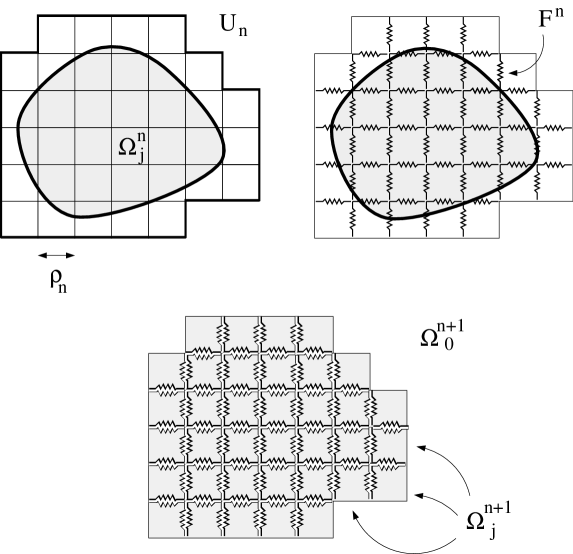
Figure 2.3. Covering $\Omega^{n}_{j}$ with squares

Replace each interior edge of the union of squares by an arc from Lemma 2.1 and call the union of the arcs $F^{n}$. See Figure 2.3 (upper right). The arcs are chosen so that we can approximate $f^{n}$ by a locally biLipschitz map on a neighborhood of $F^{n}$. Let $\Omega^{n+1}_{0}$ be the union of $\Omega^{n}_{0}$ and this neighborhood. Without loss of generality, we may assume $\Omega^{n+1}_{0}$ is bounded by a finite number of smooth closed curves $\{E^{n+1}_{j}\}$ and that we have a $2$-biLipschitz homeomorphism $f^{n+1}$ defined on $\Omega^{n+1}$ which agrees with $f^{n}$ on $\Omega^{n}_{0}\setminus U^{n}$. See Figure 2.3 (bottom). Define $f^{n+1}$ to be a diffeomorphism of the plane by extending $f^{n+1}$ to the bounded complementary components of $E^{n+1}=\partial\Omega^{n+1}_{0}$ in any way you want. Finally, note that

$$\text{diam}(f^{n+1}(E^{n+1}_{j}))\leq 2\cdot\text{diam}(f^{n}(S))\leq 2^{-n-1},$$

which is the final part of the induction hypothesis.

This completes the inductive step of the construction, i.e. given the set $E^{n}$ and mapping $\{f^{n}\}$ we have constructed $E^{n+1}$ and $\{f^{n+1}\}$ which satisfy the induction hypothesis. We now apply the following elementary lemma to the sets $F^{n}=\overline{U^{n}}$.

Lemma 2.2.

Suppose $\{F^{n}\}\subset{\mathbb{R}}^{d}$ is decreasing, nested sequence of compact sets with disjoint components $F^{n}=\cup_{j}F^{n}_{j}$, and $\lim_{n\to 0}\sup_{j}\text{diam}(F^{n}_{j})=0.$ Then $F=\cap_{n}F_{n}$ is totally disconnected. Suppose $\{g^{n}\}$ is a sequence of homeomorphisms of ${\mathbb{R}}^{d}$ to itself such that $g^{n}=g^{n+1}$ on ${\mathbb{R}}^{d}\setminus F^{n}$ and $\lim_{n\to 0}\sup_{j}\text{diam}((g^{n}(F^{n}_{j}))=0.$ Then $\{g_{n}\}$ converges uniformly to a homeomorphism $g:{\mathbb{R}}^{d}\to{\mathbb{R}}^{d}$.

We leave the proof of this to the reader. Using the lemma we see our maps converge to a homeomorphism which is locally biLipschitz off a totally disconnected set $E$. Finally, to see that $g$ is not locally biLipschitz on all of ${\mathbb{R}}^{2}$, there are several things we could do. The easiest is to define the homeomorphisms $\{f^{n}\}$ at each stage so that the limiting homeomorphism is not Hölder of any positive order. Thus it is not even quasiconformal on ${\mathbb{R}}^{2}$.

3. A flexible square

To do the construction in three dimensions, we follow the previous construction. However, when we get to the step where we replaced each edge of the covering squares by a flexible arc, we will have to replace faces of a cube by flexible surfaces. Building such surfaces is the only difficult point in extending the construction to higher dimensions.

Lemma 3.1.

Suppose $g$ is a diffeomorphism of a neighborhood of $[0,1]^{2}$ into ${\mathbb{R}}^{3}$. Suppose that $\epsilon>0$ is given. Then there is a surface $S_{1}$ and smooth mapping $G$ defined on a neighborhood of $S_{1}$ so that

1. $S_{1}$ is a topological disk which approximates $[0,1]^{2}$ to within $\epsilon$ in the Hausdorff metric.

2. If $g$ is locally $M$-biLipschitz on a neighborhood of $\partial[0,1]^{2}$ then $G$ is locally $(M+\epsilon)$-biLipschitz on $S_{1}$ and is uniformly locally biLipschitz outside an $\epsilon$-neighborhood of $\partial S_{1}$.

3. If $g$ is $M$-quasiconformal on a neighborhood of $\partial[0,1]^{2}$ then $G$ is $(M+\epsilon)$-quasiconformal on $S_{1}$.

Proof.

The basic idea is that the flexible surface can be obtained by “folding” a large square to make it oscillate, first in one direction and then in the other. We first show how to build a surface on which linear maps can be approximated.

Let $\gamma$ be the flexible arc constructed earlier and let $S_{0}$ be the surface obtained by crossing it with an interval. See Figure 3.1.

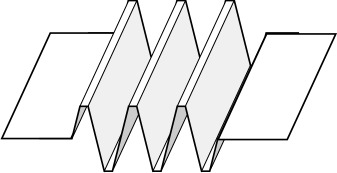
Figure 3.1. Surface flexible in one direction

Then $S_{0}$ is can be stretched (by a locally biLipschitz map) in the direction parallel to $\gamma$ and may be skewed in the the perpendicular direction. Although the figure seems to have sharp corners, one should think of this as a smooth surface on small scales (or as polygonal with very small angle between adjacent faces).

Next, tile $S_{0}$ with small squares and replace each by a copy of $S_{0}$, but now with the copy of $\gamma$ oriented in the perpendicular direction. The scale is chosen to be so small that $S_{0}$ looks flat in the small squares and so that adjacent tiles meet at very small angle. Thus adjacent tiles can be joined with only a small distortion. Since $S_{0}$ can be stretched or shrunk in one direction and the small tiles can be stretched or shrunk in the other, the resulting surface $S_{1}$, can be simultaneously stretched or shrunk in both directions by a locally biLipschitz map, i.e., we can approximate maps of the form $(x,y)\to(ax,by)$. Drawing the surface itself is a bit complicated, but Figure 3.2 gives an idea of what it looks like. The picture is a little misleading because the oscillations in different directions should be at very different scales.

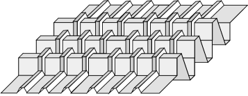
Figure 3.2. A flexible surface

We may also assume that if the “height” of the large oscillations is $\delta$ then there is a $\delta\times\delta$ flat square in each corner of $S_{1}$ and a $\delta$ wide strip along each edge in which there are only oscillations in one direction. These strips will be used below to interpolate maps defined on adjacent squares.

The horizontal or vertical stretching is easy to see. The fact that we can skew our surface (i.e., approximate maps of the form $(x,y)\to(x,y+cx)$) by a locally biLipschitz map is a little harder but is illustrated in Figure 3.3. The picture shows the surface in Figure 3.1 viewed from above. The white rectangles correspond to the horizontal pieces and the shaded rectangles to the almost vertical pieces. First we stretch the square by making the almost vertical sides horizontal. Then we apply a bounded distortion skew to each shaded rectangle. Finally, we shrink in the horizontal direction by making the shaded pieces almost vertical again.

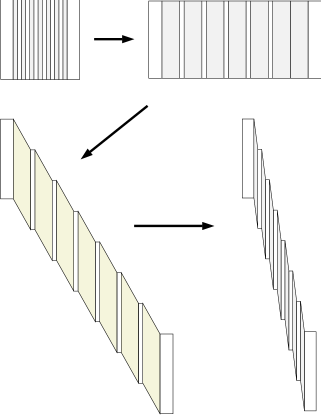
Figure 3.3. Approximating a skew map on the flexible surface

Given any linear map of a square into the plane, we now have a surface which approximates the square and a locally biLipschitz map which approximates the linear map. Moreover, the degree of approximation is controlled in terms of the size of the oscillations of the surface. In particular, the images of the boundary arcs are, up to small distortion, simply the arcs stretched (or shrunk) to the appropriate diameter, i.e., up to a small distortion, the shape of the image arc is determined by the distance between its endpoints. This is the main point which is used to glue together our approximations on adjacent flexible squares.

We now replace our smooth map $g$ by a piecewise linear approximation. Consider Figure 3.4. It shows three regions; $U_{1}$, a neighborhood of $\partial[0,1]^{2}$, (the light gray region), a square $Q=[\eta,1-\eta]^{2}$ (the dark gray area), and $U_{2}$, an open set which connects the two. Inside $U_{1}$, we leave $g$ alone. We triangulate $U_{2}$ and define an approximation to $g$ which agrees with $g$ at the vertices on the of triangulation and on the faces which meet $U_{1}$, but which is linear on the faces which hit $Q$. Since $g$ is smooth, we can do this and get a locally biLipschitz approximation with constant close to that for $g$ if we take the neighborhoods small enough.

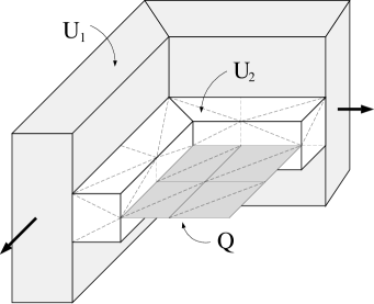
Figure 3.4. Replace $g$ by a piecewise linear approximation

Divide $Q$ into small squares and divide each into two triangles by cutting it by a diagonal. If the squares are small enough, then we can replace $g$ by an approximation that agrees with $g$ at all the vertices and which is linear on each of the triangles.

Now replace each subsquare in $Q$ with a copy of the same flexible surface, chosen so that on each square we can approximate $g$ by a locally biLipschitz map on the surface and so that our approximation agrees with $g$ at the vertices of the triangulation (First approximates the linear map on one of the two triangles whose union is the square; then apply a biLipschitz map with small distortion to “bend” the image along the diagonal to get the fourth corner to agree.)

The maps defined on adjacent squares might not match up along the common boundaries but we can fix this as follows. Along each edge of our flexible squares, we have a strip whose width is greater than the vertical size of the oscillations and in which there are only oscillations in one direction. See Figure 3.5. On the surface minus these boundary strips we simply take the restriction of the map defined above. Inside the strip, the surface is a union of rectangles and in the image, the opposite sides are perturbed by a small angle and translation (this is due to our earlier remarks that the images of the boundary arcs are determined up to small distortion by the positions of the endpoints. The two boundary arcs we are trying to glue have the same endpoints and hence are small distortions of each other.) We can divide each rectangle into two triangles and linearly interpolate the maps on the boundary arcs. See Figure 3.6. Similarly for the flat squares in the corners where four flexible squares come together. The interpolated mapping is locally biLipschitz with a uniform bound.

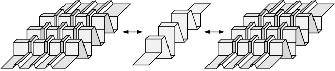
Figure 3.5. Strip adjoining adjacent squares

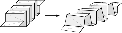
Figure 3.6. Interpolating map on strip.

Finally, we have to attach flexible squares to the boundary. When we attach a flexible square to $U_{2}$ in Figure 3.4 the boundary arc lies in one of the triangular faces where our approximation is linear. Thus the images of the arc on the face of $U_{2}$ and along the edge of the flexible square are only small distortions of each other. Thus, just as above, we may glue the mappings along a strip. See Figure 3.7.

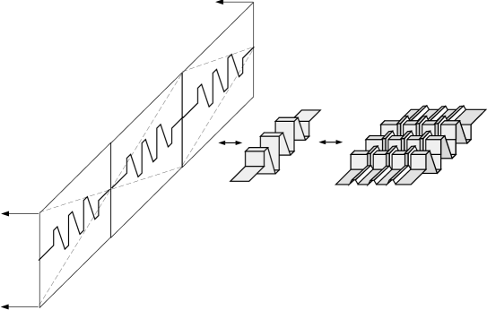
Figure 3.7. Gluing map on flexible square to the boundary values.

The proof of (3) is almost exactly as above. The only real difference is that now we may also dilate the surface by Euclidean similarities (which change the biLipschitz constant, but not the quasiconformal constant). Subdivide the square into much smaller squares so that the Jacobian of $g$ is almost constant on each square, and replace these squares by flexible surfaces. Then on each piece of the surface, we can approximate $g$ by the composition of a Euclidean dilation with the same Jacobian and a locally biLipschitz map on the surface. The definitions on adjacent squares can be matched as before, so this gives the desired approximation. ∎

In addition to building flexible surfaces which approximate a flat square, we will also want to build flexible surfaces which approximate more complicated surfaces in ${\mathbb{R}}^{3}$. For our purposes it will be enough to consider surfaces which are unions of dyadic squares, each of which is parallel to one of the three coordinate planes. It is easy to join flexible surfaces which approximate adjoining squares in the same plane, because the boundaries of the flexible surfaces match exactly. See Figure 3.8.

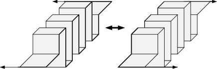
Figure 3.8. Parallel flexible squares can be joined.

A little more care is needed if the squares are not in the same plane. We choose three flexible arcs $\gamma_{1}$, $\gamma_{2}$ and $\gamma_{3}$ of vastly different scales, one corresponding to each of the coordinate directions and we use them to build three of flexible squares, (one for each of the $xy$, $yz$ and $zx$ planes) with the property that edges of these surfaces which are parallel to the given coordinate axis have the corresponding flexible arc as boundary. Thus whenever we want to join flexible surfaces corresponding to adjacent, but perpendicular, squares the corresponding edges will look the same and can be joined as in Figure 3.9 by beveling each of the surface at 45 degrees in order to join them.

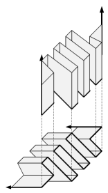
Figure 3.9. Perpendicular flexible squares can be joined.

4. A non-removable set for locally biLipschitz maps in ${{\mathbb{R}}}^{3}$

The procedure in Section 2 can now easily be adapted to construct a totally disconnected set $E$ and a homeomorphism $f$ of ${\mathbb{R}}^{3}$ to itself which is locally biLipschitz off $E$, but not even quasiconformal on all of ${\mathbb{R}}^{3}$.

Let $E^{0}$ be the unit sphere in ${{\mathbb{R}}}^{3}$, let $\Omega^{0}$ denote its unbounded complementary component and let $f^{0}$ be the identity map on $\Omega^{0}$. Extend $f^{0}$ to a diffeomorphism (which we also call $f^{0}$) of ${\mathbb{R}}^{3}$ in any way you want (later we will want the extension to have a lot of distortion). In general, we assume we have a set $E^{n}$ which is a union of $J_{n}$ components $\{E^{n}_{j}\}$, each a smooth topological $2$-sphere of diameter $\leq 2^{-n}$ bounding a topological $3$-ball $\Omega^{n}_{j}$, $j=1,\dots,J_{n}$. Denote the unbounded complementary component of $E^{n}$ by $\Omega^{n}_{0}$. Also assume we are given a homeomorphism $f^{n}$ of ${\mathbb{R}}^{3}$ which is locally biLipschitz on $\Omega^{n}_{0}$ and so that $\text{diam}(f^{n}(E^{n}_{j}))\leq 2^{-n}$.

We now describe the induction step. Let ${\cal S}^{n}$ be a collection of $\rho_{n}\times\rho_{n}$ cubes chosen from the usual lattice which covers a neighborhood $U^{n}$ of $\overline{\cup_{j}\Omega^{n}_{j}}$. The size $\rho_{n}$ should be chosen so that $\rho_{n}\leq\frac{1}{10}\min_{j\neq k}\text{dist}(E^{n}_{j},E^{n}_{k})$, and so that $\text{diam}(f^{n}(Q))\leq 2^{-n}/10$.

Replace each interior edge of the union of cubes by a oscillating curve (such as in Lemma 2.1) and approximate $f^{n}$ on a neighborhood of this arc by a locally biLipschitz mapping with a uniform constant. See Figure 4.1.

Figure 4.1. Replace edges of cubes by flexible arcs

For any face of a cube in $U^{n}$, take the four corners and consider the corresponding closed polygonal curve obtained from the union of the four arcs described above. Span this curve by a polyhedral surface $S_{1}$ which approximates the original cube face and which is a union of faces of the dyadic squares (e.g. take a smooth spanning surface and replace it by faces of dyadic cubes which hit it). Extend the map $f^{n+1}$ from the neighborhood of the boundary curve to a neighborhood of the spanning surface. The extension should be a diffeomorphism which approximates $f^{n}$. Now replace each square in the spanning surface by a copy of the flexible square constructed in Section 3. This gives a surface $S_{2}$. Then our approximation to $f^{n}$ on the spanning surface $S_{1}$ has a uniformly locally biLipschitz approximation on a neighborhood of $S_{2}$.

Let $\Omega^{n+1}_{0}$ be the union of $\Omega^{n}\setminus U^{n}$ and the open neighborhoods constructed above on which $f^{n+1}$ is defined. Then $f^{n}$ extends from $\Omega^{n}_{0}\setminus U^{n}$ to a locally biLipschitz map $f^{n+1}$ on $\Omega^{n+1}_{0}$. Let $E^{n}=\partial\Omega^{n+1}_{0}$. Without loss of generality we may take $E^{n+1}$ to be a finite union of smooth surfaces. Finally, extend $f^{n+1}$ to a diffeomorphism of of ${\mathbb{R}}^{3}$ in any way you want.

In the limit we obtain a homeomorphism $g$ of ${\mathbb{R}}^{3}$ to itself which is locally biLipschitz except on some totally disconnected set $E$. There is enough freedom in choosing the extensions at each stage that we can easily make sure that $f$ is not Hölder, so we are done. We have now constructed a totally disconnected, non-removable set for locally biLipschitz (and hence for quasiconformal) mappings. The remainder of the paper deals with modifying the construction in order to make $E$ and $f(E)$ small in the sense of Hausdorff measure.

5. Small non-removable sets for quasiconformal maps in ${\mathbb{R}}^{2}$

We now begin the process of modifying the construction so that $E$ and $f(E)$ are small, i.e., fix a function $\varphi(t)=o(t^{2})$, and show ${\cal H}^{\varphi}(E)={\cal H}^{\varphi}(f(E))=0$. This is considerable easier for quasiconformal than for locally biLipschitz mappings, so we begin with a discussion of the quasiconformal case. The construction in ${\mathbb{R}}^{3}$ only requires one extra idea, so we will first give the details in ${\mathbb{R}}^{2}$.

As before, we will define our exceptional set $E$ as a limit of sets $\{E^{n}\}$, each of which is a finite union of smooth curves $E^{n}=\cup_{j}E^{n}_{j}$ (with diameters tending to $0$ as $n\to\infty$). Our homeomorphism $f$ will be a limit of mappings $\{f^{n}\}$ which are quasiconformal on each of the finitely many components of $\Omega^{n}={\mathbb{R}}^{2}\setminus E^{n}$. This is different from what we did before, where we only defined $f^{n}$ to be “good” on the single unbounded component and extended it any we wanted to the bounded components. The maps $\{f_{n}\}$ will not be homeomorphisms because the definitions on different components of $\Omega^{n}$ will disagree on $\partial\Omega^{n}=E^{n}$. The main idea of the inductive step is to reduce the amount of disagreement at each step.

To begin the induction we start with $E^{0}=\{z:|z|=1\}$. Let $\Omega^{0}$ be the complement of $E^{0}$, let $\Omega^{0}_{0}$ be its unbounded component and $\Omega^{0}_{1}$ the bounded component. Define

$$f^{0}_{0}(z)=z,\quad z\in\Omega^{0}_{0},$$

$$f^{0}_{1}(z)=\frac{1}{2}z,\quad z\in\Omega^{0}_{1}.$$

The induction hypothesis is as follows. Suppose we are given a compact set $E^{n}$ which is a finite union of $J_{n}$ smooth closed curves, $\{E^{n}_{j}\}$, which are disjoint with disjoint interiors. Let $\Omega^{n}$ be the complement of $E^{n}$. Its unbounded component is denoted $\Omega^{n}_{0}$ and the bounded components are denoted $\Omega^{n}_{j}$, $j=1,\dots,J_{n}$. Suppose we are given diffeomorphisms $f^{n}_{j}$ on $\Omega^{n}_{j}$, $j=0,\dots,J_{n}$, which are quasiconformal with constant $M$ on each component, and $f^{n}_{j}(\Omega^{n}_{j})$ lies in $Y^{n}_{j}$, the bounded complementary component of $f^{n}_{0}(E^{n}_{j})$. See Figure 5.1

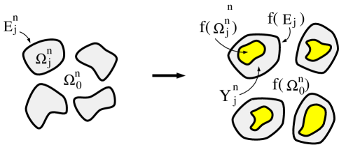
Figure 5.1. Definitions at the beginning of the induction.

What follows is a description of how to construct $f^{n+1}$ and $E^{n+1}$ from $f^{n}$ and $E^{n}$.

Step 1: Fix a very small number $\eta_{n}>0$ and for $j=1,\dots,J_{n}$ let $V^{n}_{j}$ be a smooth annular neighborhood of $E^{n}_{j}$ which is contained in

$$\{z:\text{dist}(z,E^{n}_{j})<\eta_{n}/10\}\subset\widehat{U}^{n}_{j}\equiv\{z:\text{dist}(z,E^{n}_{j})<\eta_{n}\},$$

and let $U^{n}_{j}=V^{n}_{j}\cap\Omega^{n}_{j}$. Let $U^{n}=\cup_{j}U^{n}_{j}$. See Figure 5.2.

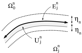
Figure 5.2. Definition of $U^{n}_{j}$.

For $j=1,\dots,J_{n}$, let

$$\widetilde{\Omega}^{n}_{j}=\Omega^{n}_{j}\setminus\overline{U^{n}},\qquad W^{n}_{j}=Y^{n}_{j}\setminus\overline{f^{n}_{j}(\widetilde{\Omega}^{n}_{j}))}.$$

See Figure 5.3.

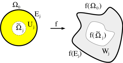
Figure 5.3. Definitions of $U^{n}_{j}$ and $W^{n}_{j}$.

Then $W^{n}=\cup_{j}W^{n}_{j}$ consists of $J_{n}$ annuli, so there is smooth diffeomorphism from $U^{n}$ to $W^{n}$, which maps $U^{n}_{j}$ diffeomorphically to $W^{n}_{j}$ and which agrees with $f^{n}_{0}$ on $E^{n}$ and with $f^{n}_{j}$ on $E^{n}_{j}$. Thus we can construct a smooth diffeomorphism $g^{n}:{\mathbb{R}}^{2}\to{\mathbb{R}}^{2}$ which agrees with $f^{n}$ on ${\mathbb{R}}^{2}\setminus U^{n}$. Now choose $\rho_{n}<\eta_{n}/100$ and consider the grid of $\rho_{n}\times\rho_{n}$ squares from the lattice $\rho_{n}{\mathbb{Z}}\times\rho_{n}{\mathbb{Z}}$. Let ${\cal S}_{n}$ be a collection of such squares which cover $U^{n}$ and are contained in $\widehat{U}^{n}$. Let $F=\cup_{Q\in{\cal S}}\partial S$. See Figure 5.4.

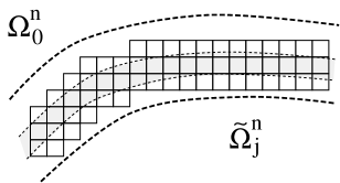
Figure 5.4. Definition of ${\cal S}_{n}$.

Step 2: We want to extend $f^{n}$ from $\Omega^{n}$ to an open connected set $\Omega^{n+1}_{0}$ which contains $\Omega^{n}_{0}$, $\cup_{j}\widetilde{\Omega}^{n}_{j}$ and a neighborhood of $F$ by approximating $g^{n}$ on a neighborhood of $F$. We can do this because any mapping on a line segment can be approximated by a mapping with bounded quasiconformal distortion on a neighborhood of the interval. In our case, it is very simple to draw a picture of the approximations. (We use straight lines instead of flexible arcs so that the resulting domain will be quasiconvex. See Section 7.)

In a neighborhood of a corner $x$ of $F$ we simply define $f^{n+1}$ to be a Euclidean similarity with the property that $f^{n+1}(x)=g^{n}(x)$.

On the line segments connecting corners we approximate $g^{n}$ by a quasiconformal map. Figure 5.5 shows how line segments may be stretched, shrunk or bent by means of a quasiconformal map with uniformly bounded dilation. Thus by approximating $g^{n}$ by a polygonal arc and using these maps to approximate each segment, we obtain the desired map.

Figure 5.5. Stretching or shrinking a line segment to approximate a polygonal arc

The only remaining observation we have to make is that the approximation can be chosen to agree with the map $f^{n}$ outside $U^{n}$. Suppose $x$ is a “boundary corner” of $F$. Then $x$ is connected by one or more grid segments to points in $\widetilde{\Omega}^{n}$. On a segment connecting $x$ and $y$ we define $f^{n+1}$ to map the arc so that $f^{n+1}$ extends both $f^{n}$ and $f^{n+1}$ to a neighborhood of the line segment. See Figure 5.6.

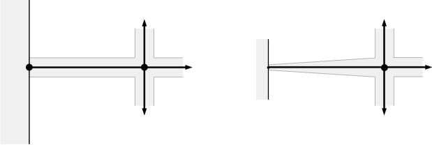
Figure 5.6. Make the connections between $f^{n+1}$ and $f^{n}$

We now have a smooth diffeomorphism $f^{n+1}$ defined on an open set $\Omega^{n+1}_{0}$ which contains $F\cup\Omega^{n}_{0}\cup_{j\geq 1}\widetilde{\Omega}^{n}_{j}$. Without loss of generality we may assume that $\partial\Omega^{n+1}_{0}$ is a finite union of smooth closed curves. Let $E^{n+1}=\partial\Omega^{n+1}_{0}$, and let $\Omega^{n+1}_{j}$, $j>1$ be an enumeration of the finitely many bounded complementary components. See Figure 5.7. To avoid confusion, let $f^{n+1}_{0}$ denote the continuous extension of $f^{n+1}$ from $\Omega^{n+1}_{0}$ to its closure.

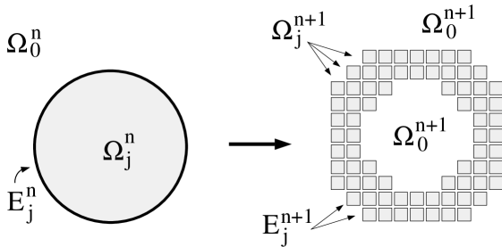
Figure 5.7. $E^{n}$ and $E^{n+1}$

To define $f^{n+1}_{j}$ on $\Omega^{n+1}_{j}$ we simply choose it to be a Euclidean (orientation preserving) similarity which maps $\overline{\Omega^{n+1}_{j}}$ into $Y^{n+1}_{j}$, the region bounded by $f^{n+1}_{0}(E^{n+1}_{j})$. See Figure 5.8.

Figure 5.8. Defining $f^{n+1}$ on the bounded components

This completes the inductive step of the construction, i.e. given the set $E^{n}$ and mapping $\{f^{n}_{j}\}$ we have constructed $E^{n+1}$ and $\{f^{n+1}_{n}\}$ which satisfy the induction hypothesis. In particular, if we let $F^{n}=\overline{\widehat{U}^{n}}$ and let $\{g^{n}\}$ be the maps constructed at the end of Step 1, they satisfy Lemma 2.2. Using the lemma we see our maps converge to a homeomorphism which is clearly quasiconformal off a Cantor set $E$. Finally, to see that $g$ is not quasiconformal on all of ${\mathbb{R}}^{2}$, there are several things we could do. The easiest is to define the homeomorphisms $\{g^{n}\}$ in Step 1 so that the limiting homeomorphism $f$ is not Hölder of any positive order.

To see that $E$ can be taken to have ${\cal H}^{\varphi}(E)=0$, fix a function $\varphi(t)=o(t)$. Since $E^{n}$ is a finite union of smooth curves, it has finite length and can be covered by $C_{n}r^{-1}$ disks $\{D_{j}\}$ of size $r$ (for all small enough $r$). Choose $r_{n}$ so small that $\varphi(r_{n})<\frac{1}{n}C_{n}^{-1}r_{n}$. In Step 1 of the construction choose $\eta_{n}<<r_{n}$ so small that $\widehat{U}_{n}\subset\cup_{j}D_{j}$. From the construction it is clear that we can take $E\subset\cup 2D_{j}$, so

$${\cal H}^{\varphi}(E)\leq\lim_{n\to\infty}2\sum_{j}\varphi(r_{n})\leq\lim_{n\to\infty}\frac{2}{n}=0,$$

as desired.

We can define the neighborhoods of $F$ to be so small at each stage that $\text{area}(W_{n})$ remains bounded away from $0$ for all $n$. This means that $f(E)$ can have positive area.

If we want to make $f(E)$ small, then instead of defining $f^{n}$ to be a similarity on $\Omega^{n}_{j}$, define it to be a conformal mapping from $\Omega^{n}_{j}$ (which is topologically a disk) to $Y^{n+1}_{j}$ (which is also a disk). Then at the next step the annular regions $W^{n+1}_{j}$ can be taken to lie in an arbitrarily thin neighborhood of $f^{n+1}_{0}(E^{n+1})$. By taking a small enough neighborhood we can obtain ${\cal H}^{\varphi}(f(E))=0$, just as above. This last step (where we have used the Riemann mapping theorem) is the only one which causes a problem in ${{\mathbb{R}}}^{3}$.

6. The quasiconformal construction in ${\mathbb{R}}^{3}$

As before let $E^{0}$ be the unit sphere, $\Omega^{0}=\Omega^{0}_{0}\cup\Omega^{0}_{1}$ its complement and

$$f^{0}_{0}(z)=z,\quad z\in\Omega^{0}_{0},$$

$$f^{0}_{1}(z)=\frac{1}{2}z,\quad z\in\Omega^{0}_{1}.$$

In general, suppose we have a compact set $E^{n}$ consisting of $J_{n}$ components $\{E^{n}_{j}\}$, each of which is a smooth surface diffeomorphic to the 2-sphere and bounding a topological 3-ball $\Omega^{n}_{j}$. Let $\Omega^{n}_{0}$ be the unbounded complementary component of $E^{n}$. Assume we have a quasiconformal map $f^{n}_{j}$, $j=0,\dots,J_{n}$ defined on each component. These maps extend smoothly across the boundaries and $f^{n}_{j}(\Omega^{n}_{j})$ is a subset of $Y^{n}_{j}$, the bounded complementary component of $f^{n}_{0}(E_{j}^{n})$.

Step 1: Define an open set $U^{n}_{j}\subset\Omega^{n}_{j}$ which is a topological annulus (i.e., homeomorphic to $S^{2}\times(0,1)$) with one boundary component $E^{n}_{j}$ and so that $U^{n}_{j}$ lies in a $\eta_{n}/10$ neighborhood of $E^{n}_{j}$. Let $U^{n}=\cup_{j}U^{n}_{j}$. For $j=1,\dots,J_{n}$, let

$$\widetilde{\Omega}^{n}_{j}=\Omega^{n}_{j}\setminus U^{n},\qquad W^{n}_{j}=Y^{n}_{j}\setminus f^{n}_{j}(\widetilde{\Omega}^{n}_{j}).$$

Then $W^{n}_{j}$ is an annulus (see Remark 6.1 concerning the annulus conjecture) and hence is diffeomorphic to $U^{n}_{j}$. Therefore there is a diffeomorphism $g^{n}$ of ${\mathbb{R}}^{3}$ to itself which agrees with $f^{n}_{j}$ on $\widetilde{\Omega}^{n}_{j}$. As before choose $\delta_{n}<\eta_{n}$ and consider a collection of cubes from a $\delta_{n}$-grid which covers $U^{n}$ and lies in a $\eta_{n}/2$ neighborhood of $E_{n}$. Let $F$ denote the union of the faces of these cubes.

Step 2: We want to define an approximation $f^{n+1}$ to $g^{n}$ on a neighborhood of $F$, but may be impossible. Instead we will define the approximation at the corners and along the edges of the cubes and then replace the faces by copies of our “flexible squares”. We then define the approximation on a neighborhood of these surfaces using Lemma 3.1.

On a neighborhood of each corner we define our approximating map $f^{n+1}$ to be a similarity which agrees with $g^{n}$ at the corner point.

On each line segment connecting two such corner points we define a uniformly quasiconformal approximation $f^{n+1}$ on some neighborhood. This is exactly the same as the two dimensional case, since we can stretch or contract a line segment by replacing the squares by cubes in Figure 2.1.

For each face of each cube, extend the approximation defined above in a neighborhood of the four edges to an approximating diffeomorphism defined on a neighborhood of the face (do this in any smooth way without worrying about the quasiconformal constant).

Next, the face of each cube is replaced by a scaled copy of a “flexible square”. The surfaces are chosen so that they lie in the neighborhoods of the faces described in the previous paragraph. By construction we have a uniformly quasiconformal approximation to $g^{n}$ on some neighborhood of these surfaces.

Let $\Omega^{n+1}_{0}$ be the open set where $f^{n+1}$ has been defined and let $E^{n+1}=\cup_{j}E^{n+1}_{j}$ be its boundary components. Without loss of generality we may assume these are smooth. Let $\Omega^{n+1}_{j}$ be the bounded complementary component of $E^{n+1}_{j}$. In each $\Omega^{n+1}_{j}$, we define a new mapping by a Euclidean similarity, so that the image of the component is contained in $Y^{n+1}_{j}$, the bounded component of the complement of $f^{n+1}(\partial\Omega^{n+1}_{j})$.

This completes the induction step. The process of passing to the limit is exactly as in the two dimensional case. Similarly, the proof that ${\cal H}^{\varphi}(E)=0$ is unchanged, except that $E$ now lies in a thin neighborhood of a surface instead of a curve, so we get an estimate for $\varphi(t)=o(t^{2})$ instead of $o(t)$.

If we want to make ${\cal H}^{\varphi}(f(E))=0$, the argument used in the two dimensional case does not work here. In that case we defined $f^{n}$ on the bounded components to be a conformal mapping using the Riemann mapping theorem, but in ${\mathbb{R}}^{3}$, this is not available to us. However, we can achieve the same result by using the following observation.

Lemma 6.1.

Suppose $\Omega$ is an open connected set with a smooth boundary and suppose $Q=[0,1]^{3}$ is the unit cube. Then there is a quasiconformal map $h$ of $Q$ onto a subdomain $\widetilde{\Omega}\subset\Omega$ such that $E=\overline{\Omega}\setminus\widetilde{\Omega}$ has $\sigma$-finite 2-dimensional measure.

Proof.

To prove this one simply takes a Whitney decomposition $\{Q_{j}\}$ for $\Omega$. Let $\widetilde{\Omega}$ be the union of the interiors of these cubes, plus small openings between certain adjacent cubes. This can be done so that $\widetilde{\Omega}$ is connected and simply connected. See Figure 6.1. It is not hard to see that $\widetilde{\Omega}$ is quasiconformally equivalent to $Q$. For example, Figure 6.2 shows how to map one cube quasiconformally to the union of two; and in such a way that the map is conformal where additional cubes might be attached. Since $\Omega\setminus\widetilde{\Omega}$ is contained in a countable number of flat squares, the final claim is obvious. ∎

Figure 6.1. A union of Whitney cubes with “openings”

Figure 6.2. Mapping a cube to a union of cubes

Using this one can get ${\cal H}^{\varphi}(f(E))=0$ (for some $\varphi(t)=o(t^{2})$) as follows. Instead of using a Euclidean similarity to map each component $\Omega^{n+1}_{j}$ into the appropriate component, use the previous lemma applied to $\Omega=Y^{n+1}_{j}$ and cube $Q$ containing $\Omega^{n+1}_{j}$. Fix a sufficiently small $r$ and choose a covering of $\Omega\setminus\widetilde{\Omega}$ with $(n\varphi(r))^{-1}$ cubes of size $r$. If the flexible surfaces making up the faces of $\Omega^{n+1}_{j}$ are close enough to the faces of $Q$, then $h(Q\setminus\Omega^{n+1}_{j})$ will be contained in a small neighborhood of $\Omega\setminus\widetilde{\Omega}$ and will also be covered by these cubes. Thus we can cover all of $f(E)$ by only $\frac{1}{n}(\varphi(r)r^{2})^{-1}$ cubes of size $r$ which is enough to give ${\cal H}^{\varphi}(f(E))=0$.

Remark 6.1: We now address the topological problem alluded to in the construction. It concerns the statement that each $W_{j}^{n}$ is a topological annulus. We would like to know that given a closed $n$-ball $B\subset{\mathbb{R}}^{n}$ and a homeomorphism $h:{\mathbb{R}}^{n}\to{\mathbb{R}}^{n}$ with $h(B)\subset\text{int(B)}$ then $B\setminus h(B)$ is homeomorphic to $S^{n-1}\times(0,1)$. This may seem obvious, but it is known as the annulus conjecture and was only proven for $n=3$ by Moise in 1952 [19] (for $n=4$ it was proven by Quinn in 1982 [20] and for $n>4$ by Kirby in 1969 [18]). Fortunately, in our case the $3$-balls in question are very explicit polyhedron and the existence of the desired homeomorphism is fairly clear. Moreover, our case fits into either the quasiconformal or biLipschitz categories and these cases are handled by work of Sullivan and of Tukia and Väisälä [21].

7. Quasiconvexity and product sets

The non-removable sets for quasiconformal mappings constructed in the two previous sections are removable for locally biLipschitz mappings. To see why, we first claim that the complement $\Omega={\mathbb{R}}^{2}\setminus E$ is quasiconvex [13], i.e., that any two points $x,y$ in $\Omega={\mathbb{R}}^{2}\setminus E$ can be connected by a path in $\Omega$ with length $\leq C|x-y|$. We may assume $x$ and $y$ are both in $\Omega^{n}_{0}$ for some $n$ and simply take the line segment between $x$ and $y$, except that whenever the segment crosses $E^{n}$ between $\Omega^{n}_{0}$ and one of the components $\Omega^{n}_{j}$, we modify it to be a polygon arc whose sides lie along the edges of cubes covering $U^{n}_{j}$. See Figure 7.1. These edges are in $\Omega^{n+1}_{0}\subset\Omega$ by construction and the modification at most doubles the length of the arc.

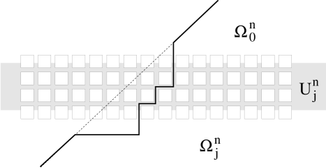
Figure 7.1. Proving $E$ has quasiconvex complement

This proves the quasiconvexity. Now apply the following result.

Lemma 7.1.

Suppose $E\subset{\mathbb{R}}^{d}$ has zero $d$-dimensional measure and $\Omega={\mathbb{R}}^{d}\setminus E$ is quasiconvex. Then any homeomorphism $f:{\mathbb{R}}^{d}\to{\mathbb{R}}^{d}$ which is locally biLipschitz on $\Omega$ is biLipschitz on all of ${\mathbb{R}}^{d}$.

Proof.

Given $x,y\in\Omega$, let $\gamma\subset\Omega$ be an arc of length $\leq C|x-y|$ connecting them. By integrating $|\nabla f|$ along $\gamma$ we see that $f$ is Lipschitz on $\Omega$ and hence on all of ${\mathbb{R}}^{d}$. This means that $f$ is absolutely continuous on lines and by the Radamacher-Stepanov theorem (e.g., Theorem 29.1 of [22]), it is differentiable almost everywhere. Since $f$ is locally biLipschitz on a set of full measure, we deduce that $f$ is quasiconformal on ${\mathbb{R}}^{d}$ (the analytic definition of quasiconformality, Theorem 34.6 of [22]). Thus $f(E)$ has zero $d$-dimensional measure, $f^{-1}$ is globally quasiconformal and also locally biLipschitz almost everywhere. Hence $F^{-1}$ is absolutely continuous on almost all lines. This implies that given two points $z,w$, we can connect them by a curve of length $\leq 2|z-w|$ along which $f^{-1}$ is absolutely continuous and has bounded derivative (just consider a family of connecting arcs which sweeps out positive measure). Integrating along the curve shows $f^{-1}$ is also Lipschitz, as desired. ∎

To build a removable set which is weakly porus, we want to show that ordinary “flat” cubes can be used in the previous construction, i.e, the “flexible surfaces” are not really needed for the quasiconformal construction. We do this by proving that a flexible surface is actually a quasiconformal image of a flat square.

Lemma 7.2.

Suppose $f$ is a diffeomorphism of $V=[0,1]^{2}\times[-\epsilon,\epsilon]$ into ${\mathbb{R}}^{3}$. Then there is a $\delta>0$ and a homeomorphism $g:U\equiv[0,1]^{2}\times[-\delta,\delta]\to{\mathbb{R}}^{3}$ such that if $A=([0,\delta]\cup[1-\delta,1])^{2}\times\delta$, and $2A=([0,2\delta]\cup[1-2\delta,1])^{2}\times\delta$, then

1. $g=f$ on $A$.

2. $g$ is uniformly quasiconformal on $U\setminus 2A$.

3. $g([0,1]^{2})$ approximates $f([0,1]^{2})$ to within $\delta$ in the Hausdorff metric.

Proof: Let $S$ be a flexible surface contained in $V$ and let $F$ be a quasiconformal approximation to $f$ on a neighborhood $V$ of $S$. We claim that there is a quasiconformal map $h$ of $U$ into $V\cup 2A$ which is the identity on $A$ and maps some subsquare of $[0,1]^{2}$ to the surface $S$. Given this, define $g=F\circ h$. It easy to verify the desired properties, so we only have to construct the map $h$.

This is easy to do in a couple of steps. First, we can quasiconformally map the square to an “expanding tower” as in Figure 7.2. The top of the tower is a large square which can be locally biLipschitz mapped to a flexible square. The sides of the expanding tower can be folded as in Figure 7.3. to agree with the oscillation on the top. The result is a surface which is close to a “straight tower”, as in Figure 7.4. Finally, the sides of the straight tower can be folded as in Figure 7.5 to “collapse” into a neighborhood of $[0,1]^{2}$, with the top mapping to $[\epsilon,1-\epsilon]^{2}$. See Figure 7.6. (The straight side should be mapped into the region bounded by the dotted line by a locally biLipschitz map before folding; then after the folding the vertical projection will be a trapezoid and the four sides will join together correctly). Composing these steps gives a uniformly quasiconformal map of a (very thin) neighborhood of $[0,1]^{2}$ to a neighborhood of the the desired surface, This proves the lemma. ∎

Figure 7.2. Step 1: Quasiconformally map square to an expanding tower.

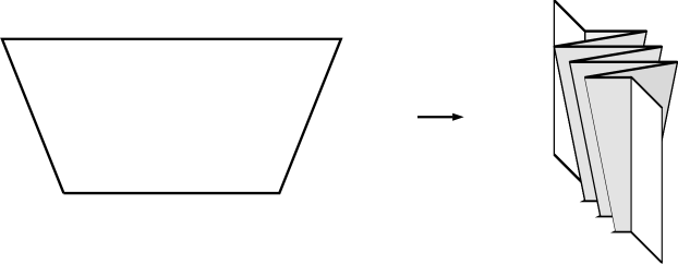
Figure 7.3. Collapsing a side of expanding tower to a neighborhood of a side of a straight tower.

Figure 7.4. Step 2: Fold the expanding tower to a straight tower with a flexible surface on top.

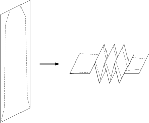
Figure 7.5. Collapsing a straight side into the base of the tower.

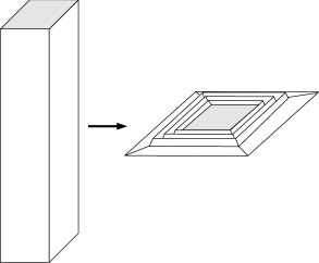
Figure 7.6. Step 3: Fold sides of straight tower to collapse it to a neighborhood of base.

The construction of non-removable sets now proceeds as before. The only difference is that instead of constructing quasiconformal approximations to arbitrary diffeomorphism, we now construct quasiconformal maps whose images approximate the images of the diffeomorphism (but the parameterizations do not necessary approximate each other). However, this is sufficient.

Using the remarks above, we see that the set we construct can be made disjoint from the faces of all dyadic cubes in ${\mathbb{}}R^{3}$. Thus the projection on each coordinate axis is totally disconnected which proves Corollary 1.5.

8. Small non-removable sets for biLipschitz maps in ${\mathbb{R}}^{2}$ and ${{\mathbb{R}}}^{3}$

We now return to building non-removable sets for locally biLipschitz maps. In this section we show how to construct such sets with small Hausdorff measure. In the next section, we show how to insure that the image has small measure.

Since the proofs in ${\mathbb{R}}^{2}$ and ${\mathbb{R}}^{3}$ are almost identical, but easier to visualize in ${\mathbb{R}}^{2}$, we will consider that case first. We will show that given a function $\varphi(t)=o(t)$, there is a totally disconnected $E\subset{\mathbb{R}}^{2}$ with ${\cal H}^{\varphi}(E)=0$ which is not removable for locally biLipschitz mappings.

Just as in Section 5, we start with $E^{0}=\{z:|z|=1\}$. Let $\Omega^{0}$ be the complement of $E^{0}$, let $\Omega^{0}_{0}$ be its unbounded component and $\Omega^{0}_{1}$ the bounded component. Define

$$f^{0}_{0}(z)=z,\quad z\in\Omega^{0}_{0},$$

$$f^{0}_{1}(z)=\frac{1}{2}z,\quad z\in\Omega^{0}_{1}.$$

The induction hypothesis is as follows. Suppose we are given a compact set $E^{n}$ which is a finite union of $J=J_{n}$ smooth closed curves, $\{E^{n}_{j}\}$. Let $\Omega^{n}$ be the complement of $E^{n}$. Its unbounded component is denoted $\Omega^{n}_{0}$ and the bounded components are denoted $\Omega^{n}_{j}$, $j=1,\dots,J_{n}$. Suppose we are given homeomorphisms $f^{n}_{j}$ on $\Omega^{n}_{j}$, $j=0,\dots,J_{n}$, which are locally biLipschitz with constant $M$ on each component, and so that $f^{n}_{j}(\Omega^{n}_{j})$ lies in $Y^{n}_{j}$, the bounded complementary component of $f^{n}_{0}(E_{j})$.

What follows is a description of how to construct $f^{n+1}$ and $E^{n+1}$ from $f^{n}$ and $E^{n}$.

Step 1: This is almost exactly as in Section 5, but with one small change. As before, fix a very small number $\eta_{n}>0$ and for $j=1,\dots,J_{n}$ let $U^{n}_{j}$ be an open topological annulus which has $E^{n}_{j}$ as its “outer” boundary component and which contains $\{z\in\Omega^{n}_{j}:\text{dist}(z,E^{n}_{j})<\eta_{n}\}$. Let $U^{n}=\cup_{j}U^{n}_{j}$. For $j=1,\dots,J_{n}$, let

$$\widetilde{\Omega}^{n}_{j}=\Omega^{n}_{j}\setminus\overline{U^{n}},\qquad W^{n}_{j}=Y^{n}_{j}\setminus f^{n}_{j}(\widetilde{\Omega}^{n}_{j})).$$

Then $W^{n}=\cup_{j}W^{n}_{j}$ consists of $J_{n}$ annuli, so there is smooth diffeomorphism from $U^{n}$ to $W^{n}$. Thus we can construct a smooth diffeomorphism $g^{n}:{\mathbb{R}}^{2}\to{\mathbb{R}}^{2}$ which agrees with $f^{n}$ on ${\mathbb{R}}^{2}\setminus U^{n}$.

In order for us to define $f^{n+1}_{j}$ to be biLipschitz later, it will be necessary to assume that $g^{n}$ is area increasing on $U^{n}$. To do this, replace $U^{n}$ by an even smaller neighborhood $\widetilde{U}^{n}_{j}\subset U^{n}_{j}$ of $E^{n}_{j}$, with

$$\widetilde{U}^{n}_{j}\subset\{z:\text{dist}(z,E^{n}_{j})<\tilde{\eta}_{n}<<\eta_{n}\}.$$

Now map $\widetilde{U}^{n}_{j}$ to $W^{n}_{j}$ by first taking the map $h:\widetilde{U}^{n}_{j}\to U^{n}_{j}$ which expands in the direction normal to $E$ and then following with the map $g:U^{n}_{j}\to W^{n}_{j}$. The first map expands volume by a factor of $\eta_{n}/\tilde{\eta}_{n}>>1$, so by selecting $\tilde{\eta}_{n}$ small enough (given the map $g$) we can assume the composition is also area expanding. See Figure 8.1.

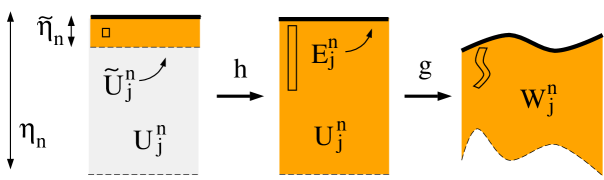
Figure 8.1. We may assume $g$ expands areas

So replacing $\eta_{n}$ and $\tilde{\eta}_{n}$ and $U^{n}_{j}$ by $\tilde{U}^{n}_{j}$ if necessary, we may assume we have a smooth mapping $g^{n}:U^{n}_{j}\to W^{n}_{j}$ which expands area.

Now choose $\delta_{n}<\eta_{n}/10$ and consider the grid of $\delta_{n}\times\delta_{n}$ squares with vertices in $\delta_{n}{\mathbb{Z}}\times\delta_{n}{\mathbb{Z}}$. Let ${\cal S}_{n}$ be a collection of such squares which cover $U^{n}$ and are contained in $\{z:\text{dist}(z,E^{n}_{j})<\eta_{n}/2\}$. Let $F=\cup_{Q\in{\cal S}}\partial S$.

Step 2: As in Sections 2 and 4 we replace the edges of the squares by flexible arcs to get a set $\widetilde{F}$, and we define $f^{n+1}$ on a neighborhood of this arcs to be a locally biLipschitz approximation to $g^{n}$ and to agree with $f^{n}$ outside $U^{n}$.

We now have a smooth diffeomorphism $f^{n+1}$ defined on an open set $\Omega^{n+1}_{0}$ which contains $\widetilde{F}\cup\cup_{j\geq 0}\widetilde{\Omega}^{n}_{j}$. Without loss of generality we may assume that $\Omega^{n+1}_{0}$ is bounded by a finite number of smooth closed curves. Let $E^{n+1}=\partial\Omega^{n+1}_{0}$, and let $\Omega^{n+1}_{j}$, $j>1$ be an enumeration of the finitely many bounded complementary components.

In Section 5, we defined $f^{n+1}_{j}$ on $\Omega^{n+1}_{j}$ simply as a Euclidean similarity which maps $\overline{\Omega^{n+1}_{j}}$ into $Y^{n+1}_{j}$. However, this map might have to shrink the component a great deal to fit it inside $Y^{n+1}_{j}$, and we lose control of the biLipschitz constant. However, because we have arranged for $g^{n}$ to be area expanding, we will be able to find a locally biLipschitz mapping of a subdomain $\widehat{\Omega}\subset\Omega^{n+1}_{j}$ into $Y^{n+1}_{j}$. First observe that since $\Omega^{n+1}_{j}$ approximates a square $Q$ in $F$ as closely as we like, its area is as close as we like to the area of the squares in $F$. Similarly, $Y^{n+1}_{j}$ is an approximation to $g(Q)$, so we may assume its area is bigger than $10\text{area}(\Omega^{n+1}_{j})$.

Furthermore, since $g$ is smooth, if we take the squares in the construction small enough then $Y^{n+1}_{j}$ will approximate a parallelogram. Choose a true parallelogram $P\subset Y^{n+1}_{j}$ and choose a collection of disjoint squares of size $\rho\times\rho$ in $P$ with connected union and which cover at least half the area of $Y^{n+1}_{j}$ (and hence more than the area of $\Omega^{n+1}_{j}$). The number $\rho$ should be chosen so $\rho<<\text{diam}(\Omega^{n+1}_{j})$. See Figure 8.2.

Figure 8.2. Squares in $Y^{n+1}_{j}$

Since $Y^{n+1}_{j}$ is connected it is possible to choose the squares so that their union is connected. Thus we can think of the collection of squares as a graph where the squares are vertices and squares that share an edge are considered adjacent in the graph. We want to label the squares $S_{1},S_{2},\dots$ so that $S_{k}$ and $S_{k+1}$ are adjacent, i.e., we want to find a Hamiltonian graph. Since the graph is connected, we can certainly find a spanning tree, but it may be impossible to find a Hamiltonian cycle. See the top picture in Figure 8.3.

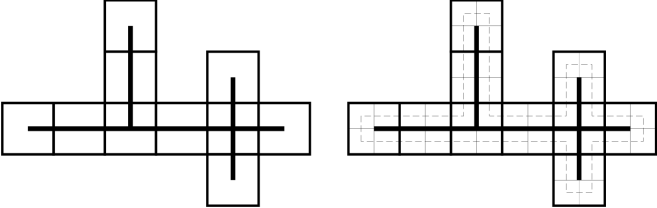
Figure 8.3. Finding a Hamiltonian cycle in the “doubled” graph of squares

However, if we replace each of our original squares by four squares of half the size then it is always possible to find a Hamiltonian path. More generally,

Lemma 8.1.

Let ${\cal S}=\{Q_{j}\}$ be a connected collection of unit squares from the usual lattice in ${\mathbb{R}}^{d}$. Let ${\cal S}^{\prime}=\{Q_{k}^{\prime}\}$ be the collection obtained by replacing each cube in ${\cal S}$ by the $2^{d}$ subcubes of side length $\frac{1}{2}$. Then the graph $G$ with vertices ${\cal S}^{\prime}$ and edges defined by adjacency of cube faces has a Hamiltonian cycle.

This is very easy by induction on the number of cubes, and we leave the proof to the reader.

Define a subdomain $\widehat{\Omega}\subset\Omega^{n+1}_{j}$ as illustrated in the upper left of Figure 8.4. This subdomain is topologically a disk, but looks like a decomposition of $\Omega^{n+1}_{j}$ into a chain of $\rho\times\rho$ squares. Because $\Omega^{n+1}_{j}$ has much smaller area than $Y^{n+1}_{j}$, the number of these squares is less than the number of squares chosen in $Y^{n+1}_{j}$ above.

Figure 8.4. A flexible subdomain $\widehat{\Omega}$ of $\Omega^{n+1}_{j}$ and biLipschitz images of its boundary and interior.

If the arcs in $\partial\widehat{\Omega}$ are made up of flexible arcs which can be shrunk by locally biLipschitz maps, then there is a locally biLipschitz map $h_{1}$ on a neighborhood of $\partial\widehat{\Omega}$ which is the identity on $\partial\Omega^{n+1}_{j}$ and which maps $\partial\widehat{\Omega}$ into $g^{-1}(Y^{n+1}_{j}\setminus P)$. Thus $h\circ g$ is a locally biLipschitz mapping of $\partial\widehat{\Omega}$ into $\partial Y^{n+1}_{j}\setminus P$. By adjoining a neighborhood of $\partial\widehat{\Omega}$ to $\Omega^{n+1}_{0}$ for each $j$ we obtain a new region $\widetilde{\Omega}^{n+1}_{0}$ and an extension of $f^{n+1}_{0}$ to the new region. The boundary of this expanded region is denoted $\widetilde{E}^{n+1}=\cup\widetilde{E}^{n+1}_{j}$, each component of which we may assume to be a smooth closed curve.

On the other hand, is easy to see that $\widehat{\Omega}$ itself can be locally biLipschitz mapped to the long narrow region in the bottom of Figure 8.4. This in turn can be locally biLipschitz mapped into the any region which is a “chain ” of similar number of similarly sized squares. In particular, it can be mapped to the squares in $P$. With a slight adjustment we can easily make the image a Jordan domain, e.g., see Figure 8.5.

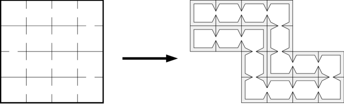
Figure 8.5. The biLipschitz image of $\widehat{\Omega}$ inside $Y^{n+1}_{j}$.

Thus on each bounded complementary component of $\widetilde{E}^{n+1}$ we have a uniformly biLipschitz mapping into the bounded complementary component of $f^{n+1}_{0}(\widetilde{E}^{n+1}_{0})$. This completes the proof of the inductive step.

Passing to a limit exactly as before we obtain a homeomorphism $f$ of ${\mathbb{R}}^{2}$ which is uniformly locally biLipschitz of a totally disconnected set $E$. Since the construction shows that we can take

$$E\subset\{z:\text{dist}(z,E_{n})\leq\eta_{n}\},$$

where $E_{n}$ is finite union of smooth curves and $\eta_{n}$ is as small as we wish (independent of $E_{n}$) it is easy to construct $E$ so ${\cal H}^{\varphi}(E)=0$.

We now make a few comments on how to modify the construction of the so that it works in ${\mathbb{R}}^{3}$. Just as above we may assume we have a mapping $g:\Omega^{n+1}_{j}\to Y^{n+1}_{j}$ which is volume expanding and almost linear. Moreover, $\Omega^{n+1}_{j}$ is a close approximation to a cube and $Y^{n+1}_{j}$ is a close approximation to a parallelepiped. We want to construct a subdomain $\widehat{\Omega}\subset\Omega^{n+1}_{j}$ so that $\Omega^{n+1}_{j}\setminus\widehat{\Omega}$ is a union of surfaces which can be mapped to a given neighborhood of $\partial\Omega^{n+1}_{j}$ by locally biLipschitz mapping, and so that there is a locally biLipschitz mapping from $\widehat{\Omega}$ to $Y^{n+1}_{j}$ which misses a given neighborhood of $\partial Y^{n+1}_{j}$. As before we find a real parallelepiped $P\subset Y^{n+1}_{j}$ and a collection of cubes in $P$ which cover half the volume of $Y^{n+1}_{j}$. As in the previous section, it may not be true that there is a Hamiltonian path in the resulting graph of cubes, but if we replace each cube by the 8 subcubes of half the size the resulting graph always has a Hamiltonian cycle.

As before, we construct $\widehat{\Omega}$ by dividing $\Omega^{n+1}_{j}$ into small “cubes” of approximately the same size as those chosen in $P$ above. Now replace the flat sides of the cubes by copies of “flexible surfaces” constructed in Section 3. The flexible surfaces are chosen so that there is biLipschitz mapping of a neighborhood of the union of faces into $g^{-1}(Y^{n+1}\setminus P)$, which is a neighborhood of $\partial\Omega^{n+1}_{j}$. Add this neighborhood to $\Omega^{n+1}_{0}$ and let $\{\widehat{\Omega}_{k}\}$ be the complement in $\Omega^{n}_{j}$.

So far $\widehat{\Omega}$ is a disjoint union of many topological balls. To make it a single ball, enumerate the components $\widehat{\Omega}_{k}$ so that $\widehat{\Omega}_{k}$ and $\widehat{\Omega}_{k+1}$ share a face and join adjacent cubes. This makes gives us a single connected component $\Omega^{n+1}_{j}$ which is topologically a ball and which can be biLipschitz mapped to a chain of cubes as in the previous section. This in turn can be biLipschitz mapped into $P\subset Y^{n+1}_{j}$, just as in the previous section.

We now have a biLipschitz map $f^{n+1}_{0}$ defined on the open set $\Omega^{n+1}_{0}$ with boundary $E^{n+1}=\cup_{j}E^{n+1}_{j}$, so that each $E^{n+1}_{j}$ is diffeomorphic to the $2$-sphere and bounds a topological $3$-ball $\Omega^{n+1}_{j}$. Moreover there is a uniformly biLipschitz map of $\Omega^{n+1}_{j}$ into $Y^{n+1}_{j}$, the bounded complementary component of $f^{n+1}_{0}(E^{n+1}_{j})$. This completes the induction step.

The proof that in the limit we get homeomorphism $f$ which is uniformly locally biLipschitz off a Cantor set $E$, is just as before. Similarly for the proof that given $\varphi(t)=o(t^{2})$ we may construct $E$ so that ${\cal H}^{\varphi}(E)=0$.

9. Making $f(E)$ small

In this section we will show how to modify the construction in order to insure ${\cal H}^{\varphi}(f(E))=0$. We start by reviewing two additional facts we will use.

The first is a result of Dacorogna and Moser [6] that if $f:\Omega_{1}\to\Omega_{2}$ is a diffeomorphism of smooth domains of equal volume, then there is another diffeomorphism $f_{0}:\Omega_{1}\to\Omega_{2}$ which agrees with $f$ on $\partial\Omega_{1}$, but which is volume preserving. (In fact, we can specify the Jacobian any smooth way we want as long the total volumes work out correctly). The second fact is a generalization of the argument used in Section 6.

Lemma 9.1.

Suppose $\Omega_{1}$ and $\Omega_{2}$ are two smooth domains in ${\mathbb{R}}^{d}$ with finite volume. Then there are subdomains $\widehat{\Omega}_{i}\subset\Omega_{i}$, $i=1,2$ so that $\Omega_{i}\setminus\widehat{\Omega}_{i}$, $i=1,2$ has finite $(d-1)$ dimensional measure and such that there is a locally biLipschitz map $f:\widehat{\Omega}_{1}\to\widehat{\Omega}_{2}$ (and the biLipschitz constant depends only on the ratio of the volumes of $\Omega_{1},\Omega_{2}$).

Proof.

First note that each smooth domain can be biLipschitz mapped to a domain which is union of cubes of side length $\rho$ which has comparable volume to the original domain. See the top of Figure 9.1.

Figure 9.1. A smooth domain can be biLipschitz mapped to a union of cubes

By replacing the cubes by cubes of half the size one can insure a Hamiltonian path in the resulting graph. Now define the subdomain by creating small openings (say of size $\rho/10$) between adjacent squares along the Hamiltonian paths. See the bottom of Figure 9.1. The resulting domains are clearly locally biLipschitz equivalent to tube of width $\rho$ and the correct volume, and hence are locally biLipschitz equivalent with each other. ∎

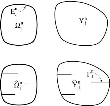
Figure 9.2. Recalling the definitions

We can now make the desired modifications of the construction. The new part of the induction hypothesis is that we have a locally biLipschitz map $f^{n}_{0}$ on $\Omega^{n}_{0}$ and locally biLipschitz maps $f^{n}_{j}$ on subdomains $\widehat{\Omega}^{n}_{j}\subset\Omega^{n}_{j}$, $j=1,\dots,J_{n}$. If $F^{n}_{j}=\overline{Y^{n}_{j}}\setminus\widehat{Y}^{n}_{j}$ (where $\widehat{Y}^{n}_{j}=f(\widehat{\Omega}_{j}^{n})$), then we also assume that $F^{n}_{j}$ has finite $d-1$ dimensional measure and $\Omega^{n}_{j}\setminus\widehat{\Omega}^{n}_{j}$ is a finite union of flat surfaces (in fact is a union of faces of dyadic cubes).

We cover both $\partial\widehat{\Omega}^{n}_{j}$ and $F^{n}=\cup_{j}F^{n}_{j}$ by balls so that the $\varphi$-sum of the radii is small (say less than $\frac{1}{n}$). Next choose a topological annulus $W^{n}_{j}\subset Y^{n}_{j}$ which covers $F^{n}_{j}$, whose outer boundary is $\partial Y^{n}_{j}$ and which is contained in the good covering of $F^{n}_{j}$ described above. Then $D^{n}_{j}=\widehat{\Omega}^{n}_{j}\setminus(f^{n}_{j})^{-1}(W^{n}_{j})$ is a Jordan subdomain of $\widehat{\Omega}^{n}_{j}$ and $\widehat{\Omega}^{n}_{j}\setminus D^{n}_{j}$ has volume comparable to $W^{n}_{j}$. By changing $f^{n}_{j}$ slightly we can assume the volumes are equal.

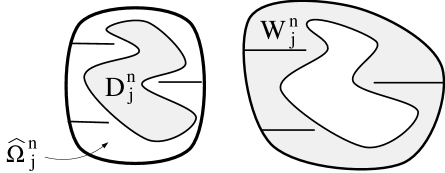
Figure 9.3. Definition of $D^{n}_{j}$ and $W^{n}_{j}$

Recall that $\partial\widehat{\Omega}^{n}_{j}$ is a finite union of flat surfaces, so we divide it up into small squares and replace each by a flexible square. The resulting domain is called $\widetilde{\Omega}^{n}_{j}$, We choose the flexible surfaces so the map $f^{n}_{0}$ can be extended to a uniformly biLipschitz map on $\Omega^{n}_{0}\cup E^{n}_{j}\cup\partial\widetilde{\Omega}^{n}_{j}$ which maps a neighborhood of $\partial\widetilde{\Omega}^{n}_{j}\cap\Omega^{n}_{j}$ into $W^{n}_{j}$.

Also, by choosing the flexible squares to be close enough to the surfaces they replace, we may assume that $\widetilde{\Omega}^{n}_{j}$ compactly contains $D^{n}_{j}$. Moreover, we may assume there is uniformly locally biLipschitz mapping $h^{n}_{j}$ from $\widetilde{\Omega}^{n}_{j}$ into a neighborhood $C^{n}_{j}$ of $\overline{D^{n}_{j}}$ which is the identity on $D^{n}_{j}$. We may also assume $\overline{C^{n}_{j}}\subset\widehat{\Omega}^{n}_{j}$. See Figure 9.4.

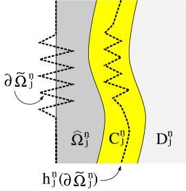
Figure 9.4. Definition of $h^{n}_{j}$

Now define a topological annulus $B^{n}_{j}$ so that (see Figure 9.5)
(1) $E^{n}_{j}$ is its outer boundary,
(2) it covers $\partial\widetilde{\Omega}^{n}_{j}\cap\Omega^{n}_{j}$,
(3) it is disjoint from $C^{n}_{j}$ and
(4) the mapping $f^{n}_{0}$ which we extended to $\partial\widetilde{\Omega}^{n}_{j}$ has a uniformly locally biLipschitz extension to $B^{n}_{j}$.

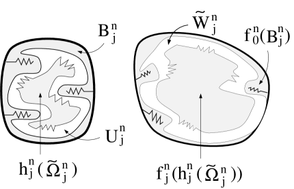
Figure 9.5. Definition of $B^{n}_{j}$ and $\widetilde{W}^{n}_{j}$

We may take the volume of $B^{n}_{j}$ to be as small as we like, in particular, smaller than half the volume of $\widehat{\Omega}^{n}_{j}\setminus C^{n}_{j}$. Thus the volume of the annulus

$$U^{n}_{j}=\widehat{\Omega}^{n}_{j}\setminus(B^{n}_{j}\cup h^{n}_{j}(\widetilde{\Omega}^{n}_{j}))$$

is comparable to the volume of the annulus

$$\widetilde{W}^{n}_{j}=W^{n}_{j}\setminus(f^{n}_{0}(B^{n}_{j})\cup f^{n}_{j}\circ h^{n}_{j}(\widetilde{\Omega}^{n}_{j})).$$

Then $U^{n}_{j}$ and $W^{n}_{j}$ are annuli of comparable volume (independent of $n$) and we have a locally biLipschitz map $f^{n}_{0}$ from the outer boundary component (i.e., $E^{n}_{j}$) of $U^{n}_{j}$ to the outer boundary of $\widetilde{W}^{n}_{j}$ and we have locally biLipschitz maps $f^{n}_{j}\circ h^{n}_{j}$ of the bounded complementary component of each $U^{n}_{j}$ to the corresponding bounded complementary component of $\widetilde{W}^{n}_{j}$.

We now use the result of Dacorogna and Moser [6] described at the beginning of this section to find diffeomorphisms $g_{j}:U^{n}_{j}\to W^{n}_{j}$ which extend $f^{n}_{0}$ and $f^{n}_{j}$ on the two boundary components and which multiply volumes by a constant factor (the ratio of the volumes).

Now proceed as before, covering $U^{n}$ by cubes, replacing the faces by flexible surfaces, approximating $g_{j}$ on these surfaces and getting in the end components $\Omega^{n+1}_{j}$ and $Y^{n+1}_{j}$ which have comparable volumes. For each component $\Omega^{n+1}_{j}$ we use Lemma 9.1 to define a subdomain $\widehat{\Omega}_{j}$ which can be mapped into a subdomain of $Y^{n+1}_{j}$.

This completes the induction. Since we began the inductive step by insuring that our construction took place within a good covering, it is easy to see that the limiting set $E$ and homeomorphism $f$ satisfy ${\cal H}^{\varphi}(E)={\cal H}^{\varphi}(f(E))=0$.

As a final remark we observe that Corollary 1.2 is almost immediate. If $f:\Omega_{1}\to\Omega_{2}$ is a diffeomorphism, then we can write $\Omega_{1}$ as a union of cubes so that $f$ is close to linear on each cube. We replace the faces of these cubes by flexible surfaces and apply the construction and we obtain the desired homeomorphism. Because the diffeomorphism may change volumes, we can only get a quasiconformal approximation. If $\Omega_{1}$ and $\Omega_{2}$ are diffeomorphic by a volume preserving map then the construction of the last two sections applies and we can get a locally bi-Lipschitz approximation.

References

- [1] L. Ahlfors and A. Beurling. Conformal invariants and function theoretic null sets. Acta Math., 83:101–129, 1950.
- [2] L. Antoine. Sur la possibité d’étrendre l’homeomorphic de deux figures à leur voisinage. Comptes Rendu Acad. Sci. Paris, 171:661–663, 1920.
- [3] A.S. Besicovitch. On the definition of tangents to sets of infinite linear measure. Proc. Camb. Phil. Soc., 52:20–29, 1956.
- [4] C.J. Bishop. Some homeomorphisms of the sphere conformal off a curve. Ann. Acad. Sci. Fenn, 19:323–338, 1994.
- [5] L. Carleson. On null-sets for continuous analytic functions. Ark. Mat., 1:311–318, 1950.
- [6] B. Dacorogna and J. Moser. On a partial differential equation involving the Jacobian determinate. Ann. Inst. Henri Poincaré; analyse non linéaire, 7:1–26, 1990.
- [7] G. David. Solutions de l’equation de Beltrami. 71, 1987.
- [8] F.W. Gehring. The definitions and exceptional sets for quasiconformal mappings. Ann. Acad. Sci. Fenn., Ser. A. I. Math., 281:1–28, 1960.
- [9] F.W. Gehring. Injectivity of quasi-isometries. Comment. Math. Helv., 57:202–220, 1982.
- [10] F.W. Gehring and O. Martio. Quasiextremal distance domains and extension of quasiconformal mappings. J. Analyse Math., 45:181–206, 1985.
- [11] F.W. Gehring and J. Väisälä. Hausdorff dimension and quasiconformal mappings. J. London Math. Soc., 6:504–512, 1971.
- [12] J. Heinonen and P. Koskela. Definitions of quasiconformality. Invent. Math., 120:61–79, 1995.
- [13] J. Heinonen and P. Koskela. Quasiconformal maps in metric spaces with controlled geometry. 1996. Preprint 191, Univ. Jyväskylä.
- [14] J.G. Hocking and G.S. Young. Topology. Addison-Wesley, 1961.
- [15] F. John. On quasi-isometric mappings. Comm. Pure Appl. Math., pages 77–110, 1968.
- [16] R. Kaufman. Fourier-Steiltjes coefficients and continuation of functions. Ann. Acad. Sci. Fenn., 9:27–31, 1984.
- [17] R. Kaufman and J.-M. Wu. On removable sets for quasiconformal mappings. Ark. Math., 34:141–158, 1996.
- [18] R.C. Kirby. Stable homeomorphisms and the annulus conjecture. Ann. Math., 89:575–582, 1969.
- [19] E.E. Moise. Affine structures in -manifolds v: the triangulations theorem and hauptvermutung. Ann. Math., 56:96–114, 1952.
- [20] F. Quinn. Ends of maps. iii: dimensions 4 and 5. J. Diff. Geo., 17:503–521, 1982.
- [21] P. Tukia and J. Väisälä. Lipschitz and quasiconformal approximation and extension. Ann. Acad. Sci. Fenn., 6:303–342, 1981.
- [22] J. Väisälä. Lectures on -dimensional quasiconformal mappings. Lecture Notes in Math. 229. Springer-Verlag, 1971.
- [23] J. Väisälä. Homeomorphisms of bounded length distortion. Ann. Acad. Sci. Fenn., 12:303–312, 1987.
- [24] J. Väisälä. Quasiconformal maps of cylindrical domains. Acta Math., 162:201–225, 1989.
- [25] J.-M. Wu. Removability of sets for quasiconformal mappings and Sobolev spaces. 1996. to appear in Complex Variables.