Continued fraction TBA and functional relations
in XXZ model at root of unity

Abstract

Thermodynamics of the spin $\frac{1}{2}$ XXZ model is studied in the critical regime using the quantum transfer matrix (QTM) approach. We find functional relations indexed by the Takahashi-Suzuki numbers among the fusion hierarchy of the QTM’s ($T$-system) and their certain combinations ($Y$-system). By investigating analyticity of the latter, we derive a closed set of non-linear integral equations which characterize the free energy and the correlation lengths for both $\langle\sigma_{j}^{+}\sigma_{i}^{-}\rangle$ and $\langle\sigma_{j}^{z}\sigma_{i}^{z}\rangle$ at any finite temperatures. Concerning the free energy, they exactly coincide with Takahashi-Suzuki’s TBA equations based on the string hypothesis. By solving the integral equations numerically the correlation lengths are determined, which agrees with the earlier results in the low temperature limit.

PACS: 05.30.-d, 05.50.+q, 05.70.-a
Keywords: XXZ model; Correlation length; Quantum transfer matrix; Functional relations; Takahashi-Suzuki numbers; Thermodynamic Bethe ansatz

1 Introduction

In this paper we study the spin $\frac{1}{2}$ XXZ model at finite temperature based on the recently developed quantum transfer matrix (QTM) approach [2]–[17]. We shall deal with the “root of unity” case in the gap-less regime. Namely, the anisotropy parameter has the form $\Delta=\cos\!\frac{\pi}{p_{0}}$ with $p_{0}$ any rational number not less than 2. (See (2.1).) We derive the non-linear integral equations that characterize the free energy and the correlation lengths for both $\langle\sigma^{+}_{j}\sigma^{-}_{i}\rangle$ and $\langle\sigma^{z}_{j}\sigma^{z}_{i}\rangle$ at any finite temperatures.

Thermodynamics of the XXZ model is a classical and by no means fresh problem at least as far as the free energy is concerned. It goes back to 1972 that Takahashi and Suzuki [18] took the thermodynamic Bethe ansatz (TBA) approach [19] to the free energy based on the elaborate string hypothesis. They selected, as allowed lengths of strings, a special sequence of integers $n_{j}$ which we call the Takahashi-Suzuki (TS) numbers. The resulting free energy yields correct physical behaviours in many respects. Actually this is one of the best known example among many successful applications of the TBA and string hypotheses. However there is also some controversy in string hypotheses themselves [20, 21, 22], in view of which those successes are rather mysterious.

This is one of our motivations to revisit the XXZ model with the recent QTM method. It integrates many ideas in the statistical mechanics and solvable models [1]–[17] and has a number of advantages over the traditional TBA approach. It only relies on certain analyticity of the QTM, which can easily be confirmed much more convincingly by numerics. Moreover it enables us to systematically calculate the correlation lengths beyond the free energy for a wide range of temperatures. See [12] for $\Delta>1$ case. Roughly, the QTM method goes as follows. First one transforms the 1D quantum system into an integrable 2D classical system based on the general equivalence theorem [1, 2]. The QTM $T_{1}$ is a transfer matrix propagating in the cross channel of the latter. Despite that the original 1D Hamiltonian $H$ is critical, the QTM $T_{1}$ can be made to have a gap. Therefore the formidable sum $\mbox{Tr}e^{-\beta H}$ ($\beta=1/k_{B}T$ : $T$ is temperature) can be expressed as its single eigenvalue which is largest in the magnitude. Furthermore the correlation lengths are obtained from the ratio of the largest and the sub-leading eigenvalues of $T_{1}$. To evaluate them actually, one must however recognize a price to pay; now the QTM $T_{1}(u)$ itself becomes dependent on the fictitious Trotter number $N$ through its size and also a coupling constant as $T_{1}(u=\mbox{const}\frac{\beta}{N})$ [6]–[10]. This makes it difficult to determine the spectra of $T_{1}$ by a naive numerical extrapolation as $N\rightarrow\infty$. A crucial idea to overcome this is to equip the QTM with another variable $v$ and to exploit the Yang-Baxter integrability with respect to it; $[T_{1}(u,v),T_{1}(u,v^{\prime})]=0$ [11]. Here $u$ and $v$ play the role of the (inverse) temperature and the spectral parameter, respectively. Furthermore one introduces some auxiliary functions of $v$, which should realize somewhat miraculous features. Their appropriate combinations should have a nice analyticity that encodes the information on the Bethe ansatz roots of $T_{1}(u,v)$. Once this is achieved, one can derive a non-linear integral equation which efficiently determines the sought eigenvalues of $T_{1}$. The Trotter limit $N\rightarrow\infty$ can thereby be taken analytically. The most essential step in this method is to invent such auxiliary functions and their appropriate combinations. There are some interesting variety of choices for them in various models [12]–[17].

Back to the XXZ model our finding is that such auxiliary functions can be given by the QTM’s $\{T_{n_{j}-1}|\,n_{j}:\mbox{TS numbers}\}$, which is the subset of the known fusion hierarchy of commuting transfer matrices whose dimensions of the auxiliary spaces are precisely the TS numbers $n_{j}$. We will show that $\{T_{n_{j}-1}\}$ satisfy functional relations among themselves ($T$-system) and so do their certain ratios $\{Y_{j}\}$ an elaborate one ($Y$-system). See (4.9)-(4.9). Especially there is a special identity (4.2) among $\{T_{n_{j}-1}\}$ that holds only at rational values of $p_{0}$ and makes the $Y$-system close finitely. Besides the peculiarity at general roots of unity, such use of the fusion hierarchy as the auxiliary functions originates in the studies of finite size corrections [23, 24].

As for the free energy we thus obtain the integral equations identical with Takahashi-Suzuki’s TBA equations but totally independently of their string hypothesis. We shall further study the second and the third largest eigenvalues of $T_{1}$ for $p_{0}$ integer. They are related to the correlation length $\xi$ of $\langle\sigma^{+}_{j}\sigma^{-}_{i}\rangle$ and $\langle\sigma^{z}_{j}\sigma^{z}_{i}\rangle$, respectively. In contrast with the largest eigenvalue, now the zeros of the $T_{n_{j}-1}$ come into the “physical strip” spoiling the nice analyticity. Nevertheless we manage to identify their patterns and derive the “excited state TBA equations”. Solving them numerically we determine the curve $\xi=\xi(\beta)$. Especially the low temperature asymptotics $\lim_{\beta\rightarrow\infty}\xi(\beta)/\beta$ agrees with the known result [12, 25] with high accuracy for the both correlations.

Our formulation here using the 2 variable QTM $T_{1}(u,v)$ and fusion hierarchies is based on [11, 16]. There are similar approaches in the context of integrable QFT’s in a finite volume [26, 27, 28].

It has been known for some time that solutions of $Y$-systems can curiously be constructed from $T$-systems [23, 29]. By now this connection has been generalized to arbitrary non-twisted affine algebra $X^{(1)}_{r}$ for the associated $Y$-system [30] and the $T$-system [29]. (See also [31].) In this sense, our results here display a further connection of such sort for $U_{q}(\widehat{sl}(2))$ at $q$ general root of unity.

The layout of the paper is as follows. In section 2 we formulate the XXZ model at finite temperature in terms of the QTM $T_{1}$. In section 3 we give the fusion hierarchy $\{T_{n-1}\}$ of QTM’s and their eigenvalues. A functional relation ($T$-system) valid for general $p_{0}$ is also given. In section 4 we construct the $Y$-system out of the $T$-system. The former closes finitely due to the special functional relation (4.2) valid only for rational $p_{0}$. In section 5 we derive integral equations for the free energy, and in section 6 for the correlation lengths of $\langle\sigma^{+}_{j}\sigma^{-}_{i}\rangle$ and $\langle\sigma^{z}_{j}\sigma^{z}_{i}\rangle$. Section 7 is a discussion. Appendix A recalls the definition of the TS numbers and the related data. Appendices B and C contain a check of the analyticity of the $Y$-functions for the free energy. Appendix D is devoted to the free fermion case $p_{0}=2$, which needs a separate treatment.

2 Quantum transfer matrix

The Hamiltonian of spin $\frac{1}{2}$ one dimensional XXZ model on a periodic lattice with $L$ sites is

$$H = \sum_{j=1}^{L}H_{j\,j+1},$$

$$H_{j\,j+1} = \frac{J}{4}\left(\sigma_{j}^{x}\sigma_{j+1}^{x}+\sigma_{j}^{y}\sigma_{j+1}^{y}+\Delta(\sigma_{j}^{z}\sigma_{j+1}^{z}-1)\right).$$ (2.1)

Here $\sigma_{j}^{x},\sigma_{j}^{y},\sigma_{j}^{z}$ are the local spin operators (Pauli matrices) at the $j$-th lattice site and $J$ is a real coupling constant. We shall consider the model with the anisotropy parameter $\Delta$ in the critical region $-1<\Delta<1$. Due to the invariance of the spectrum of (2.1) under the transformation $(J,\Delta)\rightarrow(-J,-\Delta)$, we can further restrict the range to $0\leq\Delta<1$ and introduce the parametrization:

$$\Delta = \cos\theta\quad 0<\theta\leq\frac{\pi}{2},$$ (2.2)

$$p_{0} = \frac{\pi}{\theta}\quad p_{0}\geq 2.$$ (2.3)

The model is associated with the quantum group $U_{q}(\widehat{sl}(2))$ at $q=e^{\pi i/p_{0}}$.

In order to consider its thermodynamics we relate it to the six vertex model. This is a two dimensional classical system whose Boltzmann weights are given by

$$\begin{picture}(22.0,10.0)(0.0,10.0)\put(4.0,10.0){\line(1,0){12.0}} \put(10.0,4.0){\line(0,1){12.0}} \put(10.0,10.0){\oval(2.5,2.5)[bl]} \put(0.0,9.0){{\scriptsize$\pm 1$}} \put(9.0,1.5){{\scriptsize$\pm 1$}} \put(16.5,9.0){{\scriptsize$\pm 1$}} \put(9.0,16.9){{\scriptsize$\pm 1$}} \put(7.0,7.0){{\scriptsize$v$}} \end{picture}=\frac{[v+2]}{[2]},\quad\begin{picture}(22.0,10.0)(0.0,10.0)\put(4.0,10.0){\line(1,0){12.0}} \put(10.0,4.0){\line(0,1){12.0}} \put(10.0,10.0){\oval(2.5,2.5)[bl]} \put(0.0,9.0){{\scriptsize$\pm 1$}} \put(9.0,1.5){{\scriptsize$\mp 1$}} \put(16.5,9.0){{\scriptsize$\pm 1$}} \put(9.0,16.9){{\scriptsize$\mp 1$}} \put(7.0,7.0){{\scriptsize$v$}} \end{picture}=\frac{[v]}{[2]},\quad\begin{picture}(22.0,10.0)(0.0,10.0)\put(4.0,10.0){\line(1,0){12.0}} \put(10.0,4.0){\line(0,1){12.0}} \put(10.0,10.0){\oval(2.5,2.5)[bl]} \put(0.0,9.0){{\scriptsize$\pm 1$}} \put(9.0,1.5){{\scriptsize$\mp 1$}} \put(16.5,9.0){{\scriptsize$\mp 1$}} \put(9.0,16.9){{\scriptsize$\pm 1$}} \put(7.0,7.0){{\scriptsize$v$}} \end{picture}=1,\\$$ (2.4)

where

$$[v]=\frac{\sin\frac{\theta}{2}v}{\sin\frac{\theta}{2}}.$$ (2.5)

Let $V$ be a two dimensional irreducible module over $U_{q}(\widehat{sl}(2))$. As is well known the quantum $R$-matrix $R\in\mbox{End}(V\otimes V)$ with the above matrix elements and the spectral parameter $v$ satisfies the Yang-Baxter equation (YBE) (cf.(3.3)). To relate the six vertex model with the XXZ model, consider a two dimensional square lattice with $N$ rows and $L$ columns. We shall assume that $N$ is even throughout. Define the (auxiliary) transfer matrix $T_{A}(u,v)$ as

$$T_{A}(u,v)=\mbox{Tr}_{V_{1}\otimes V_{2}}\Biggl{(}\quad\quad\begin{picture}(60.0,15.0)(0.0,15.0)\put(0.0,10.0){\line(1,0){60.0}} \put(0.0,20.0){\line(1,0){60.0}} \put(10.0,5.0){\line(0,1){20.0}} \put(20.0,5.0){\line(0,1){20.0}} \put(40.0,5.0){\line(0,1){20.0}} \put(50.0,5.0){\line(0,1){20.0}} \put(10.0,10.0){\oval(2.5,2.5)[bl]} \put(20.0,10.0){\oval(2.5,2.5)[bl]} \put(40.0,10.0){\oval(2.5,2.5)[bl]} \put(50.0,10.0){\oval(2.5,2.5)[bl]} \put(10.0,20.0){\oval(2.5,2.5)[br]} \put(20.0,20.0){\oval(2.5,2.5)[br]} \put(40.0,20.0){\oval(2.5,2.5)[br]} \put(50.0,20.0){\oval(2.5,2.5)[br]} \put(1.0,7.0){{\scriptsize$u-iv$}} \put(11.0,7.0){{\scriptsize$u-iv$}} \put(31.0,7.0){{\scriptsize$u-iv$}} \put(41.0,7.0){{\scriptsize$u-iv$}} \put(11.0,17.0){{\scriptsize$u+iv$}} \put(21.0,17.0){{\scriptsize$u+iv$}} \put(41.0,17.0){{\scriptsize$u+iv$}} \put(51.0,17.0){{\scriptsize$u+iv$}} \put(8.5,1.0){{\footnotesize$V^{\prime}_{1}$}} \put(18.5,1.0){{\footnotesize$V^{\prime}_{2}$}} \put(38.5,1.0){{\footnotesize$V^{\prime}_{L-1}$}} \put(48.5,1.0){{\footnotesize$V^{\prime}_{L}$}} \put(-5.0,8.5){{\footnotesize$V_{2}$}} \put(-5.0,17.5){{\footnotesize$V_{1}$}} \end{picture}\quad\Biggr{)}.\\$$ (2.6)

See also Fig.1. Here and in what follows $V_{1}=\cdots=V_{N}=V^{\prime}_{1}=\cdots=V^{\prime}_{L}=V$. Operators diagrammatically shown as in (2.6) are always assumed to act on the states in the bottom line to transfer them into those in the upper line. Using the identity ($P_{j\,j+1}$ is the permutation operator acting on $V_{j}\otimes V_{j+1}$),

$$R_{j\,j+1}(0)\frac{d}{dv}R_{j\,j+1}(v)\bigg{|}_{v=0} = P_{j\,j+1}\frac{d}{dv}R_{j\,j+1}(v)\bigg{|}_{v=0}$$

$$= \frac{\theta}{J\sin\theta}\left(H_{j\,j+1}+\frac{J}{2}\Delta\right),$$

we expand $T_{A}(u,0)$ as

$$T_{A}(u,0)=1+\frac{2\theta u}{J\sin\theta}\left(H+\frac{JL\Delta}{2}\right)+O(u^{2}).$$ (2.7)

This formula represents as an equivalence of the XXZ model and the six vertex model. In fact we can go further to the finite temperature case. From (2.7) it follows that

$$\exp\left(-\beta\left(H+\frac{JL}{2}\Delta\right)\right)=\lim_{N\to\infty}T_{A}(u_{N},0)^{\frac{N}{2}},\quad\quad u_{N}=-\frac{\beta J\sin\theta}{\theta N}.$$ (2.8)

Thus the free energy per site $f$ of the XXZ model is given by

$$f=-\lim_{L\to\infty}\lim_{N\to\infty}\frac{1}{L\beta}\ln\left(\mbox{Tr}_{V^{\otimes L}}T_{A}(u_{N},0)^{\frac{N}{2}}\right)-\frac{J}{2}\Delta.$$ (2.9)

However, eigenvalues of the transfer matrix $T_{A}(u_{N},0)$ are infinitely degenerate in the limit $u_{N}\stackrel{{\scriptstyle N\to\infty}}{{\longrightarrow}}0$, therefore the the trace renders a serious problem. To avoid this, we introduce the following trick; we rotate the lattice by $90^{\circ}$ (see Fig.1) and rewrite the free energy as

$$f=-\lim_{L\to\infty}\lim_{N\to\infty}\frac{1}{L\beta}\ln\left(\mbox{Tr}_{V^{\otimes N}}T_{1}(u_{N},0)^{L}\right)-\frac{J}{2}\Delta,$$ (2.10)

where

$$T_{1}(u,v)=\mbox{Tr}_{V^{\prime}_{1}}\Biggl{(}\quad\quad\begin{picture}(60.0,10.0)(0.0,10.0)\put(0.0,10.0){\line(1,0){60.0}} \put(10.0,5.0){\line(0,1){10.0}} \put(20.0,5.0){\line(0,1){10.0}} \put(40.0,5.0){\line(0,1){10.0}} \put(50.0,5.0){\line(0,1){10.0}} \put(10.0,10.0){\oval(2.5,2.5)[tr]} \put(20.0,10.0){\oval(2.5,2.5)[br]} \put(40.0,10.0){\oval(2.5,2.5)[tr]} \put(50.0,10.0){\oval(2.5,2.5)[br]} \put(11.0,12.0){{\scriptsize$u+iv$}} \put(21.0,7.0){{\scriptsize$u-iv$}} \put(41.0,12.0){{\scriptsize$u+iv$}} \put(51.0,7.0){{\scriptsize$u-iv$}} \put(8.5,1.0){{\footnotesize$V_{1}$}} \put(18.5,1.0){{\footnotesize$V_{2}$}} \put(38.5,1.0){{\footnotesize$V_{N-1}$}} \put(48.5,1.0){{\footnotesize$V_{N}$}} \put(-5.0,8.5){{\footnotesize$V^{\prime}_{1}$}} \end{picture}\quad\Biggr{)}.\\$$ (2.11)

Figure 1: Relation between $T_{A}(u,v)$ and $T_{1}(u,v).$

We call $T_{1}(u,v)$ the quantum transfer matrix (QTM). Note that due to the YBE (3.3), the QTM is commutative as long as the $u$ variable is taken same:

$$[T_{1}(u,v),T_{1}(u,v^{\prime})]=0.$$

From now on, we write the $k$-th largest eigenvalue of the matrix $T_{1}(u,v)$ as $T^{(k)}_{1}(u,v)$. Since the two limits are exchangeable as proved in [2, 3], we take the limit $L\to\infty$ first. Noting that there is a finite gap between $\lim_{N\to\infty}T^{(1)}_{1}(u_{N},0)$ and $\lim_{N\to\infty}T^{(2)}_{1}(u_{N},0)$, we have

$$f=-\frac{1}{\beta}\lim_{N\to\infty}\ln T_{1}^{(1)}(u_{N},0)-\frac{J}{2}\Delta.$$ (2.12)

Namely, the problem of describing the thermodynamics of one dimensional quantum systems reduces to finding the largest eigenvalue of the QTM of two dimensional finite systems (to be exact, finite in the vertical direction only). Equation (2.12) is a finite temperature extension of the equation (2.7).

In this approach, the thermodynamical completeness $-\lim_{\beta\rightarrow 0}\beta f=\ln 2$ follows easily from $T^{(1)}_{1}(0,0)=2$, which is obvious from $R_{12}(0)=P_{12}$. (As for the combinatorial completeness see [32] including the higher spin cases.)

Most significantly this method makes it possible to calculate some correlation length $\xi_{k}$ ($k\geq 2$) at finite temperature. To see this let $Q_{i}=1\otimes\cdots\otimes Q\otimes\cdots\otimes 1\in\hbox{End}(V^{\otimes L})$ be a local operator acting on the $i$-th site $V^{\prime}_{i}$ via $Q=\sum_{\ell,\ell^{\prime}=\pm 1}Q_{\ell^{\prime},\ell}E_{\ell^{\prime},\ell}$. Here $E_{\ell^{\prime},\ell}$ denotes the $2$ by $2$ elementary matrix and $Q_{\ell^{\prime},\ell}$ is the matrix element. ($\sigma^{z}=E_{1,1}-E_{-1,-1},\sigma^{+}=E_{1,-1},\sigma^{-}=E_{-1,1}$.) Given $Q$ we introduce the operator $S(Q|u,v)\in\hbox{End}(V^{\otimes N})$ by

$$S(Q|u,v)=\sum_{\ell,\ell^{\prime}=\pm 1}Q_{\ell^{\prime},\ell}\Biggl{(}\quad\begin{picture}(60.0,10.0)(0.0,10.0)\put(0.0,10.0){\line(1,0){60.0}} \put(10.0,5.0){\line(0,1){10.0}} \put(20.0,5.0){\line(0,1){10.0}} \put(40.0,5.0){\line(0,1){10.0}} \put(50.0,5.0){\line(0,1){10.0}} \put(10.0,10.0){\oval(2.5,2.5)[tr]} \put(20.0,10.0){\oval(2.5,2.5)[br]} \put(40.0,10.0){\oval(2.5,2.5)[tr]} \put(50.0,10.0){\oval(2.5,2.5)[br]} \put(11.0,12.0){{\scriptsize$u+iv$}} \put(21.0,7.0){{\scriptsize$u-iv$}} \put(41.0,12.0){{\scriptsize$u+iv$}} \put(51.0,7.0){{\scriptsize$u-iv$}} \put(8.5,1.0){{\footnotesize$V_{1}$}} \put(18.5,1.0){{\footnotesize$V_{2}$}} \put(38.5,1.0){{\footnotesize$V_{N-1}$}} \put(48.5,1.0){{\footnotesize$V_{N}$}} \put(-3.0,8.5){{\footnotesize$\ell$}} \put(62.0,8.5){{\footnotesize$\ell^{\prime}$}} \end{picture}\quad\Biggr{)}.\\$$

Then for the local operators $Q_{i},P_{j}\in\hbox{End}(V^{\otimes L})$ their finite temperature correlation function is expressed as

$$\langle P_{j}Q_{i}\rangle = \lim_{L\rightarrow\infty}\frac{\mbox{Tr}_{V^{\otimes L}}\,P_{j}Q_{i}\exp(-\beta H)}{\mbox{Tr}_{V^{\otimes L}}\,\exp(-\beta H)}$$

$$= \lim_{N\to\infty}\lim_{L\to\infty}\frac{\mbox{Tr}_{V^{\otimes N}}\left(S(P|u_{N},0)T_{1}(u_{N},0)^{j-i-1}S(Q|u_{N},0)T_{1}(u_{N},0)^{L+i-j-1}\right)}{\mbox{Tr}_{V^{\otimes N}}T_{1}(u_{N},0)^{L}},$$

where we have exchanged the two limits. Suppose that $Q^{(k)}$ and $Q^{(k)\dagger}$ are the operators such that the matrix elements of $S(Q^{(k)}|u_{N},0)$ and $S(Q^{(k)\dagger}|u_{N},0)$ between the eigenspaces for $T^{(1)}_{1}(u_{N},0)$ and $T^{(k^{\prime})}_{1}(u_{N},0)$ are zero for $1\leq k^{\prime}<k$ and nonzero for $k^{\prime}=k$. Then setting $(P,Q)=(Q^{(k)\dagger},Q^{(k)})$ in the above, we have

$$\langle Q^{(k){\dagger}}_{j}Q^{(k)}_{i}\rangle\sim\lim_{N\to\infty}\left(\frac{T^{(k)}_{1}(u_{N},0)}{T^{(1)}_{1}(u_{N},0)}\right)^{j-i}\qquad k\geq 2,\,j\gg i.$$

Fitting this with $\exp(-(j-i)/\xi_{k})$ in the limit $j\gg i$ we have

$$\frac{1}{\xi_{k}}=-\lim_{N\to\infty}\ln\left|\frac{T^{(k)}_{1}(u_{N},0)}{T^{(1)}_{1}(u_{N},0)}\right|.$$ (2.13)

As seen in section 6, $\xi_{2}$ and $\xi_{3}$ are the correlation lengths of $\langle\sigma_{j}^{+}\sigma_{i}^{-}\rangle$ ($Q^{(2)}=\sigma^{-}$) and $\langle\sigma_{j}^{z}\sigma_{i}^{z}\rangle$ ($Q^{(3)}=\sigma^{z}$), respectively.

3 $T$-system

To study $T_{1}(u,v)$, we embed it into a more general family of transfer matrices and explore the functional relations that govern the total system. For this we consider the fusion hierarchy $\{T_{n-1}(u,v)\}$ defined by

$$T_{n-1}(u,v)=\mbox{Tr}\Biggl{(}\begin{picture}(60.0,10.0)(0.0,10.0)\put(0.0,10.0){\line(1,0){1.0}}\put(2.0,10.0){\line(1,0){1.0}}\put(4.0,10.0){\line(1,0){1.0}}\put(6.0,10.0){\line(1,0){1.0}}\put(8.0,10.0){\line(1,0){1.0}}\put(10.0,10.0){\line(1,0){1.0}}\put(12.0,10.0){\line(1,0){1.0}}\put(14.0,10.0){\line(1,0){1.0}}\put(16.0,10.0){\line(1,0){1.0}}\put(18.0,10.0){\line(1,0){1.0}}\put(20.0,10.0){\line(1,0){1.0}}\put(22.0,10.0){\line(1,0){1.0}}\put(24.0,10.0){\line(1,0){1.0}}\put(26.0,10.0){\line(1,0){1.0}}\put(28.0,10.0){\line(1,0){1.0}}\put(30.0,10.0){\line(1,0){1.0}}\put(32.0,10.0){\line(1,0){1.0}}\put(34.0,10.0){\line(1,0){1.0}}\put(36.0,10.0){\line(1,0){1.0}}\put(38.0,10.0){\line(1,0){1.0}}\put(40.0,10.0){\line(1,0){1.0}}\put(42.0,10.0){\line(1,0){1.0}}\put(44.0,10.0){\line(1,0){1.0}}\put(46.0,10.0){\line(1,0){1.0}}\put(48.0,10.0){\line(1,0){1.0}}\put(50.0,10.0){\line(1,0){1.0}}\put(52.0,10.0){\line(1,0){1.0}}\put(54.0,10.0){\line(1,0){1.0}}\put(56.0,10.0){\line(1,0){1.0}}\put(58.0,10.0){\line(1,0){1.0}} \put(10.0,5.0){\line(0,1){10.0}} \put(20.0,5.0){\line(0,1){10.0}} \put(40.0,5.0){\line(0,1){10.0}} \put(50.0,5.0){\line(0,1){10.0}} \put(10.0,10.0){\oval(2.5,2.5)[tr]} \put(20.0,10.0){\oval(2.5,2.5)[br]} \put(40.0,10.0){\oval(2.5,2.5)[tr]} \put(50.0,10.0){\oval(2.5,2.5)[br]} \put(11.0,12.0){{\scriptsize$u+iv$}} \put(21.0,7.0){{\scriptsize$u-iv$}} \put(41.0,12.0){{\scriptsize$u+iv$}} \put(51.0,7.0){{\scriptsize$u-iv$}} \put(8.5,1.0){{\footnotesize$V_{1}$}} \put(18.5,1.0){{\footnotesize$V_{2}$}} \put(38.5,1.0){{\footnotesize$V_{N-1}$}} \put(48.5,1.0){{\footnotesize$V_{N}$}} \end{picture}\Biggr{)},\\$$ (3.1)

where the trace is over the $n$ dimensional irreducible auxiliary space depicted by the dotted line. To be explicit, we give the constituent fusion Boltzmann weights.

$$\begin{picture}(22.0,10.0)(0.0,10.0)\put(4.0,10.0){\line(1,0){1.1}}\put(5.8,10.0){\line(1,0){1.1}}\put(7.6,10.0){\line(1,0){1.1}}\put(9.4,10.0){\line(1,0){1.1}}\put(11.2,10.0){\line(1,0){1.1}}\put(13.0,10.0){\line(1,0){1.1}}\put(14.8,10.0){\line(1,0){1.1}} \put(10.0,4.0){\line(0,1){12.0}} \put(10.0,10.0){\oval(2.5,2.5)[bl]} \put(2.0,9.0){{\scriptsize$j$}} \put(9.0,1.5){{\scriptsize$\pm 1$}} \put(16.5,9.0){{\scriptsize$j$}} \put(9.0,16.9){{\scriptsize$\pm 1$}} \put(7.0,7.0){{\scriptsize$v$}} \end{picture}=\begin{picture}(22.0,10.0)(0.0,10.0)\put(4.0,10.0){\line(1,0){1.1}}\put(5.8,10.0){\line(1,0){1.1}}\put(7.6,10.0){\line(1,0){1.1}}\put(9.4,10.0){\line(1,0){1.1}}\put(11.2,10.0){\line(1,0){1.1}}\put(13.0,10.0){\line(1,0){1.1}}\put(14.8,10.0){\line(1,0){1.1}} \put(10.0,4.0){\line(0,1){12.0}} \put(10.0,10.0){\oval(2.5,2.5)[br]} \put(2.0,9.0){{\scriptsize$j$}} \put(9.0,1.5){{\scriptsize$\pm 1$}} \put(16.5,9.0){{\scriptsize$j$}} \put(9.0,16.9){{\scriptsize$\pm 1$}} \put(11.0,7.0){{\scriptsize$v$}} \end{picture}=\frac{[v+1\pm(n+1-2j)]}{[2]},$$

$$\begin{picture}(22.0,10.0)(0.0,10.0)\put(4.0,10.0){\line(1,0){1.1}}\put(5.8,10.0){\line(1,0){1.1}}\put(7.6,10.0){\line(1,0){1.1}}\put(9.4,10.0){\line(1,0){1.1}}\put(11.2,10.0){\line(1,0){1.1}}\put(13.0,10.0){\line(1,0){1.1}}\put(14.8,10.0){\line(1,0){1.1}} \put(10.0,4.0){\line(0,1){12.0}} \put(10.0,10.0){\oval(2.5,2.5)[bl]} \put(2.0,9.0){{\scriptsize$j$}} \put(7.0,1.5){{\scriptsize$j-j^{\prime}$}} \put(16.5,9.0){{\scriptsize$j^{\prime}$}} \put(7.0,16.9){{\scriptsize$j^{\prime}-j$}} \put(7.0,7.0){{\scriptsize$v$}} \end{picture}=\epsilon_{jj^{\prime}}\frac{\sqrt{[2\mbox{min}(j,j^{\prime})][2n-2\mbox{min}(j,j^{\prime})]}}{[2]},$$

$$\begin{picture}(22.0,10.0)(0.0,10.0)\put(4.0,10.0){\line(1,0){1.1}}\put(5.8,10.0){\line(1,0){1.1}}\put(7.6,10.0){\line(1,0){1.1}}\put(9.4,10.0){\line(1,0){1.1}}\put(11.2,10.0){\line(1,0){1.1}}\put(13.0,10.0){\line(1,0){1.1}}\put(14.8,10.0){\line(1,0){1.1}} \put(10.0,4.0){\line(0,1){12.0}} \put(10.0,10.0){\oval(2.5,2.5)[br]} \put(2.0,9.0){{\scriptsize$j$}} \put(7.0,1.5){{\scriptsize$j^{\prime}-j$}} \put(16.5,9.0){{\scriptsize$j^{\prime}$}} \put(7.0,16.9){{\scriptsize$j-j^{\prime}$}} \put(11.0,7.0){{\scriptsize$v$}} \end{picture}=\epsilon^{\prime}_{jj^{\prime}}\frac{\sqrt{[2\mbox{min}(j,j^{\prime})][2n-2\mbox{min}(j,j^{\prime})]}}{[2]}.$$

Here $j,j^{\prime}\in\{1,\ldots,n\}$ and $|j-j^{\prime}|=1$. $\epsilon_{jj^{\prime}},\epsilon^{\prime}_{jj^{\prime}}$ are arbitrary parameters such that $\epsilon_{jj^{\prime}}\epsilon_{j^{\prime}j}=\epsilon^{\prime}_{jj^{\prime}}\epsilon^{\prime}_{j^{\prime}j}=1$. If they are 1, the six vertex case $n=2$ of these weights reduce to (2.4) under the identification of $j=1$ and $2$ states with $+1$ and $-1$, respectively. The Boltzmann weights satisfy the YBE:

$$\begin{picture}(50.0,25.0)(0.0,25.0)\put(10.0,5.0){\line(1,2){20.0}} \put(40.0,5.0){\line(-1,2){20.0}} \put(5.0,12.5){\line(1,0){1.0}}\put(7.0,12.5){\line(1,0){1.0}}\put(9.0,12.5){\line(1,0){1.0}}\put(11.0,12.5){\line(1,0){1.0}}\put(13.0,12.5){\line(1,0){1.0}}\put(15.0,12.5){\line(1,0){1.0}}\put(17.0,12.5){\line(1,0){1.0}}\put(19.0,12.5){\line(1,0){1.0}}\put(21.0,12.5){\line(1,0){1.0}}\put(23.0,12.5){\line(1,0){1.0}}\put(25.0,12.5){\line(1,0){1.0}}\put(27.0,12.5){\line(1,0){1.0}}\put(29.0,12.5){\line(1,0){1.0}}\put(31.0,12.5){\line(1,0){1.0}}\put(33.0,12.5){\line(1,0){1.0}}\put(35.0,12.5){\line(1,0){1.0}}\put(37.0,12.5){\line(1,0){1.0}}\put(39.0,12.5){\line(1,0){1.0}}\put(41.0,12.5){\line(1,0){1.0}}\put(43.0,12.5){\line(1,0){1.0}} \bezier{50}(11.0,12.5)(11.0,11.0)(12.5,10.0)\bezier{50}(32.5,12.5)(33.5,8.5)(37.5,10.0)\bezier{50}(23.7,32.5)(25.0,31.0)(26.3,32.5)\put(8.0,8.0){{\scriptsize$v$}} \put(33.0,5.0){{\scriptsize$v^{\prime}$}} \put(27.0,32.0){{\scriptsize$v^{\prime}-v$}} \end{picture}=\begin{picture}(50.0,25.0)(0.0,25.0)\put(20.0,5.0){\line(1,2){20.0}} \put(30.0,5.0){\line(-1,2){20.0}} \put(5.0,37.5){\line(1,0){1.0}}\put(7.0,37.5){\line(1,0){1.0}}\put(9.0,37.5){\line(1,0){1.0}}\put(11.0,37.5){\line(1,0){1.0}}\put(13.0,37.5){\line(1,0){1.0}}\put(15.0,37.5){\line(1,0){1.0}}\put(17.0,37.5){\line(1,0){1.0}}\put(19.0,37.5){\line(1,0){1.0}}\put(21.0,37.5){\line(1,0){1.0}}\put(23.0,37.5){\line(1,0){1.0}}\put(25.0,37.5){\line(1,0){1.0}}\put(27.0,37.5){\line(1,0){1.0}}\put(29.0,37.5){\line(1,0){1.0}}\put(31.0,37.5){\line(1,0){1.0}}\put(33.0,37.5){\line(1,0){1.0}}\put(35.0,37.5){\line(1,0){1.0}}\put(37.0,37.5){\line(1,0){1.0}}\put(39.0,37.5){\line(1,0){1.0}}\put(41.0,37.5){\line(1,0){1.0}}\put(43.0,37.5){\line(1,0){1.0}} \bezier{50}(33.5,37.5)(33.5,36.0)(35.0,35.0)\bezier{50}(10.0,37.5)(11.0,33.5)(15.0,35.0)\bezier{50}(23.7,12.5)(25.0,11.0)(26.3,12.5)\put(31.0,32.0){{\scriptsize$v$}} \put(8.0,30.0){{\scriptsize$v^{\prime}$}} \put(28.0,11.0){{\scriptsize$v^{\prime}-v$}} \end{picture},\begin{picture}(50.0,25.0)(0.0,25.0)\put(10.0,5.0){\line(1,2){20.0}} \put(40.0,5.0){\line(-1,2){20.0}} \put(5.0,12.5){\line(1,0){1.0}}\put(7.0,12.5){\line(1,0){1.0}}\put(9.0,12.5){\line(1,0){1.0}}\put(11.0,12.5){\line(1,0){1.0}}\put(13.0,12.5){\line(1,0){1.0}}\put(15.0,12.5){\line(1,0){1.0}}\put(17.0,12.5){\line(1,0){1.0}}\put(19.0,12.5){\line(1,0){1.0}}\put(21.0,12.5){\line(1,0){1.0}}\put(23.0,12.5){\line(1,0){1.0}}\put(25.0,12.5){\line(1,0){1.0}}\put(27.0,12.5){\line(1,0){1.0}}\put(29.0,12.5){\line(1,0){1.0}}\put(31.0,12.5){\line(1,0){1.0}}\put(33.0,12.5){\line(1,0){1.0}}\put(35.0,12.5){\line(1,0){1.0}}\put(37.0,12.5){\line(1,0){1.0}}\put(39.0,12.5){\line(1,0){1.0}}\put(41.0,12.5){\line(1,0){1.0}}\put(43.0,12.5){\line(1,0){1.0}} \bezier{50}(33.5,12.5)(33.5,13.5)(35.0,15.0)\bezier{50}(10.0,12.5)(11.5,16.0)(15.0,15.0)\bezier{50}(23.7,32.5)(25.0,31.0)(26.3,32.5)\put(8.5,14.0){{\scriptsize$v$}} \put(30.0,13.0){{\scriptsize$v^{\prime}$}} \put(27.0,32.0){{\scriptsize$v-v^{\prime}$}} \end{picture}=\begin{picture}(50.0,25.0)(0.0,25.0)\put(20.0,5.0){\line(1,2){20.0}} \put(30.0,5.0){\line(-1,2){20.0}} \put(5.0,37.5){\line(1,0){1.0}}\put(7.0,37.5){\line(1,0){1.0}}\put(9.0,37.5){\line(1,0){1.0}}\put(11.0,37.5){\line(1,0){1.0}}\put(13.0,37.5){\line(1,0){1.0}}\put(15.0,37.5){\line(1,0){1.0}}\put(17.0,37.5){\line(1,0){1.0}}\put(19.0,37.5){\line(1,0){1.0}}\put(21.0,37.5){\line(1,0){1.0}}\put(23.0,37.5){\line(1,0){1.0}}\put(25.0,37.5){\line(1,0){1.0}}\put(27.0,37.5){\line(1,0){1.0}}\put(29.0,37.5){\line(1,0){1.0}}\put(31.0,37.5){\line(1,0){1.0}}\put(33.0,37.5){\line(1,0){1.0}}\put(35.0,37.5){\line(1,0){1.0}}\put(37.0,37.5){\line(1,0){1.0}}\put(39.0,37.5){\line(1,0){1.0}}\put(41.0,37.5){\line(1,0){1.0}}\put(43.0,37.5){\line(1,0){1.0}} \bezier{50}(11.0,37.5)(11.0,39.0)(12.5,40.0)\bezier{50}(32.5,37.5)(34.0,41.0)(37.5,40.0)\bezier{50}(23.7,12.5)(25.0,11.0)(26.3,12.5)\put(31.0,39.0){{\scriptsize$v$}} \put(7.0,38.0){{\scriptsize$v^{\prime}$}} \put(28.0,11.0){{\scriptsize$v-v^{\prime}$}} \end{picture}\\$$ (3.3)

From the picture (3.1) one sees that the members of the fusion hierarchy are all commutative for the same $u$:

$$[T_{n-1}(u,v),T_{n^{\prime}-1}(u,v^{\prime})]=0,$$

due to the $R$-matrix intertwining the $n$ and $n^{\prime}$ dimensional representations. Thus they can be simultaneously diagonalized and the eigenvalues (also written as $T_{n-1}(u,v)$) are readily obtained in the dressed vacuum form:

$$T_{n-1}(u,v) =\sum_{j=1}^{n}\phi\bigl{(}v-i(u+n+2-2j)\bigr{)}\phi\bigl{(}v+i(u-n+2j)\bigr{)}$$ (3.4)

$$\times\frac{Q(v+in)Q(v-in)}{Q\bigl{(}v+i(2j-n)\bigr{)}Q\bigl{(}v+i(2j-n-2)\bigr{)}},$$

$$\phi(v) =\biggl{(}\frac{\mbox{sh}\frac{\theta}{2}v}{\sin\theta}\biggr{)}^{\frac{N}{2}},$$ (3.5)

$$Q(v) =\prod_{j=1}^{m}\mbox{sh}\frac{\theta}{2}(v-\omega_{j}).$$ (3.6)

Here $m\in\{0,1,\ldots,N/2\}$ is the quantum number counting the $(-1)$-states on odd sites and $(+1)$-states on even sites. The dressed vacuum form is built upon the pseudo vacuum state $\bigl{(}(+1)\otimes(-1)\bigr{)}^{\otimes\frac{N}{2}}$, which corresponds to $m=0$. $\{\omega_{j}\}$ is a solution of the Bethe ansatz equation (BAE):

$$-\Biggl{(}\frac{\mbox{sh}\frac{\theta}{2}\bigl{(}\omega_{j}+i(u+2)\bigr{)}\mbox{sh}\frac{\theta}{2}(\omega_{j}-iu)}{\mbox{sh}\frac{\theta}{2}\bigl{(}\omega_{j}-i(u+2)\bigr{)}\mbox{sh}\frac{\theta}{2}(\omega_{j}+iu)}\Biggr{)}^{\frac{N}{2}}=\frac{Q(\omega_{j}+2i)}{Q(\omega_{j}-2i)}.$$ (3.7)

The largest eigenvalue of $T_{1}(u,v)$ lies in the sector $m=N/2$. Note that $T_{-1}(u,v)=0$ and $T_{0}(u,v)=\phi(v-i(u+1))\phi(v+i(u+1))$. An important property is the periodicity

$$T_{n-1}(u,v)=T_{n-1}(u,v+2p_{0}i).$$ (3.8)

Let us present the functional relations among the fusion hierarchy. For any $v\in{\bf C}$ and integers $n\geq y\geq 1$, the following is valid, which we call the $T$-system.

$$T_{n-1}(v+iy)T_{n-1}(v-iy)=T_{n+y-1}(v)T_{n-y-1}(v)+T_{y-1}(v+in)T_{y-1}(v-in).$$ (3.9)

Hereafter we shall often omit the common $u$ variable to simplify the notation. The proof of this equation is direct by using the expression (3.4). Representation theoretically, it is a simple consequence of the general exact sequence in [33] as explained in [29] for $y=1$. In general the $T$-system (3.9) extends over infinitely many transfer matrices. However, as we shall see in the next section, for rational $p_{0}$ there is a special functional relation (4.2) that makes the associated $Y$-system closes finitely.

4 $Y$-system at Root of Unity

From now on, we shall concentrate on the case when $p_{0}>2$ is a rational number and treat the free fermion case $p_{0}$=2 separately in Appendix D. Consider the continued fraction expansion of $p_{0}$

$$p_{0}=\nu_{1}+\frac{1}{\displaystyle\nu_{2}+\frac{1}{\displaystyle\frac{\ddots}{\displaystyle\nu_{\alpha-1}+\frac{1}{\displaystyle\nu_{\alpha}}}}},$$ (4.1)

which specifies $\alpha\geq 1$ and $\nu_{1},\ldots,\nu_{\alpha}\in{\bf Z}_{\geq 1}$. From the assumption $p_{0}>2$, we have $\nu_{1}\geq 2$. In fact $\nu_{1}=2$ is allowed only if $\alpha\geq 2$, and $p_{0}=\nu_{1}\geq 3$ is assumed if $\alpha=1$.

In Appendix A we recall the sequences of numbers $\{m_{j}\}_{j=0}^{\alpha+1},\{p_{j}\}_{j=0}^{\alpha+1},\{y_{j}\}_{j=-1}^{\alpha},\{z_{j}\}_{j=-1}^{\alpha}$ and $\{n_{j}\}_{j\geq 1}$ introduced in [18]. The last one is the TS numbers. We shall also introduce its slight rearrangement $\{\widetilde{n}_{j}\}_{j\geq 1}$ and a similar sequence $\{w_{j}\}_{j\geq 1}$ related to the “parity” of the TS strings. They are all specified uniquely from $p_{0}$. With those definitions we now describe a functional relation of the $T_{n-1}(v)$, which is valid only at the root of unity and is relevant to our subsequent argument.

$$T_{y_{\alpha}+y_{\alpha-1}-1}(v)=T_{y_{\alpha}-y_{\alpha-1}-1}(v)+2(-1)^{mz_{\alpha}}T_{y_{\alpha-1}-1}(v+iy_{\alpha}).$$ (4.2)

Here $m$ is the number of the BAE roots in (3.6). The proof is straightforward by using (3.4), (A.8) and $Q(v+2iy_{\alpha})=(-1)^{mz_{\alpha}}Q(v)$. When $\alpha=1$ hence $p_{0}=\nu_{1}$, (4.2) reduces to a simple relation $T_{\nu_{1}}(v)=T_{\nu_{1}-2}(v)+2(-1)^{m}T_{0}(v+i\nu_{1})$.

For $1\leq j\leq j_{max}:=m_{\alpha}-1$, let $0\leq r\leq\alpha-1$ be the unique integer satisfying $m_{r}\leq j<m_{r+1}$. Set

$$Y_{j}(v) =\frac{T_{{\tilde{n}}_{j+1}+y_{r}-1}(v+iw_{j}p_{0})T_{{\tilde{n}}_{j+1}-y_{r}-1}(v+iw_{j}p_{0})}{T_{y_{r}-1}(v+i{\widetilde{n}}_{j+1}+iw_{j}p_{0})T_{y_{r}-1}(v-i{\widetilde{n}}_{j+1}+iw_{j}p_{0})},$$ (4.3)

$$1+Y_{j}(v) =\frac{T_{{\tilde{n}}_{j+1}-1}(v+iy_{r}+iw_{j}p_{0})T_{{\tilde{n}}_{j+1}-1}(v-iy_{r}+iw_{j}p_{0})}{T_{y_{r}-1}(v+i{\widetilde{n}}_{j+1}+iw_{j}p_{0})T_{y_{r}-1}(v-i{\widetilde{n}}_{j+1}+iw_{j}p_{0})},$$ (4.4)

$$K(v) =\frac{(-1)^{mz_{\alpha}}T_{{\tilde{n}}_{j_{max}}-1}(v+iw_{j_{max}}p_{0})}{T_{y_{\alpha-1}-1}(v+iy_{\alpha}+iw_{j_{max}}p_{0})},$$ (4.5)

where in (4.5) ${\widetilde{n}}_{j_{max}}=y_{\alpha}-y_{\alpha-1}$ and $w_{j_{max}}=z_{\alpha}-z_{\alpha-1}-1$ in accordance with (A.10) and (Appendix A   Takahashi-Suzuki (TS) numbers). We also set $Y_{0}(v)=0$ and $Y_{-1}(v)=\infty$. Thanks to the $T$-system (3.9), (4.3) and (4.4) are equivalent. We find that $\{Y_{j}(v)\}_{j=1}^{m_{\alpha}-1}$ and $K(v)$ close among the following finite set of functional relations, which we call the $Y$-system.

Theorem 1

For $$m_{r-1}\leq j\leq m_{r}-2\,\,(1\leq r\leq\alpha),$$ (4.9)

$$Y_{j}(v+ip_{r})Y_{j}(v-ip_{r})=\bigl{(}1+Y_{j-1}(v)\bigr{)}^{1-2\delta_{jm_{r-1}}}\bigl{(}1+Y_{j+1}(v)\bigr{)},$$

for $$j=m_{r}-1\,\,(1\leq r\leq\alpha-1),$$

$$Y_{j}(v+ip_{r}+ip_{r+1})Y_{j}(v+ip_{r}-ip_{r+1})Y_{j}(v-ip_{r}+ip_{r+1})Y_{j}(v-ip_{r}-ip_{r+1})$$

$$=\biggl{\{}\bigl{(}1+Y_{j-1}(v+ip_{r+1})\bigr{)}\bigl{(}1+Y_{j-1}(v-ip_{r+1})\bigr{)}\biggr{\}}^{1-2\delta_{1\nu_{r}}}\bigl{(}1+Y_{j+1}(v+ip_{r})\bigr{)}$$

$$\times\bigl{(}1+Y_{j+1}(v-ip_{r})\bigr{)}\bigl{(}1+Y_{j}(v+ip_{r}-ip_{r+1})\bigr{)}\bigl{(}1+Y_{j}(v-ip_{r}+ip_{r+1})\bigr{)},$$

$$1+Y_{m_{\alpha}-1}(v)=\left(1+K(v)\right)^{2},$$

$$K(v+ip_{\alpha})K(v-ip_{\alpha})=1+Y_{m_{\alpha}-2}(v).$$

This can be proved by combining the $T$-systems (3.9), (4.2) with the definitions of $\{m_{j}\},\{p_{j}\},\{y_{j}\},\{\widetilde{n}_{j}\}$ and $\{w_{j}\}$ in Appendix A. When $\nu_{r}=1$, (4.9) is void and (4.9) holds for $j=m_{r}-1=m_{r-1}$. See (A.1).

In the case $p_{0}\in{\bf Z}_{\geq 3}$, the $Y$-system has a simple form ($1\leq j\leq p_{0}-2$)

$$Y_{j}(v+i)Y_{j}(v-i)=(1+Y_{j-1}(v))(1+Y_{j+1}(v)),$$ (4.10)

$$1+Y_{p_{0}-1}(v)=(1+K(v))^{2},$$ (4.11)

$$K(v+i)K(v-i)=1+Y_{p_{0}-2}(v),$$ (4.12)

where

$$Y_{j}(v)=\frac{T_{j+1}(v)T_{j-1}(v)}{T_{0}(v+i(j+1))T_{0}(v-i(j+1))},$$ (4.13)

$$1+Y_{j}(v)=\frac{T_{j}(v+i)T_{j}(v-i)}{T_{0}(v+i(j+1))T_{0}(v-i(j+1))},$$ (4.14)

$$K(v)=(-)^{m}\frac{T_{p_{0}-2}(v)}{T_{0}(v+ip_{0})}$$ (4.15)

for $1\leq j\leq p_{0}-2$. Due to the property of the TS-number, $Y_{1}(v)$ and $1+Y_{1}(v)$ are always given by setting $j=1$ in (4.13) and (4.14) for arbitrary $p_{0}>2$.

A similar $Y$-system has been considered in [34] in a perturbed CFT context.

5 Integral equation for free energy

Let $|k\rangle$ be the eigenvector corresponding to the $k$-th largest eigenvalue $T^{(k)}_{1}(u,v)$ of $T_{1}(u,v)$. We define the $k$-th (not necessarily $k$-th largest) eigenvalue $T^{(k)}_{n-1}(u,v)$ of the auxiliary QTM $T_{n-1}(u,v)$ by $T_{n-1}(u,v)|k\rangle=T^{(k)}_{n-1}(u,v)|k\rangle$. Let $\{Y^{(k)}_{j}\}$ (and $K^{(k)}$) be the $Y$-functions constructed from $\{T^{(k)}_{n-1}\}$ as in (4.3) – (4.5). In this section, we study the analyticity of $\{Y^{(1)}_{j}(u,v)\}$ and $K^{(1)}(u,v)$ in the complex $v$-plane. Then we derive the integral equations which characterize the free energy.

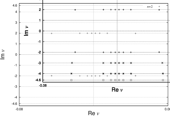
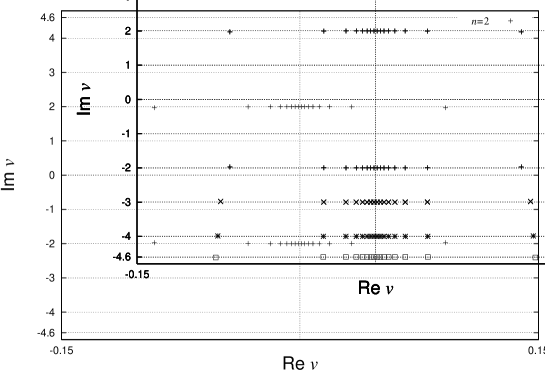
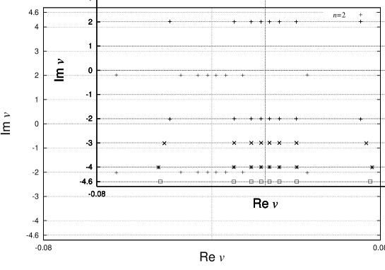
Figure 2: Location of zeros of $T^{(1)}_{n-1}(u,v)$ for $n=2,3,4,5$, $p_{0}=\frac{24}{5}=4.8$, $u=-0.01$, $N=16$ (first), $N=32$ (second) and $u=0.01$, $N=16$ (third). The zeros are located on an almost straight line $\Im v=\pm n\,\,\hbox{mod }2p_{0}$. The deviation from the line is $\sim 10^{-2}$.

An advantage in the present approach lies in the fact that the analytic assumption given below can be explicitly checked numerically keeping the Trotter number $N$ finite. We have performed numerical studies with various values of $p_{0}$, $\beta$ and $N$ in determining the location zeros of fusion QTM’s. For example, the zeros for $T^{(1)}_{n-1}(u,v)$ for $p_{0}=\frac{24}{5},u=\pm 0.01$, $n$=2,3,4,5 $N=16$ and $N=32$ are plotted in Fig 2. Guided by them we have the following for $u$ small (typically $|u|\sim 0.01$).

Conjecture 1

All the zeros of $T^{(1)}_{n-1}(u,v)$ are located on the almost straight lines $\Im v=\pm n\hbox{ mod }2p_{0}$.

This coincides with the observation in the XXX model if one forgets the periodicity $2p_{0}$ in the imaginary direction. It is also consistent with the functional relation (3.9). The deviation from the straight line is very small ($\sim 10^{-2}$ at most) as seen in the figures. It becomes smaller as $u\rightarrow 0$. Once Conjecture 1 is assumed, we can identify the strips in the complex $v$-plane in which $Y^{(1)}_{j}(v)$ or $1+Y_{j}^{(1)}(v)$ are analytic, nonzero and have constant asymptotics at $v=\pm\infty$. We call this property ANZC. In Appendix B we verify that $Y^{(1)}_{j}(v)$, for example, is ANZC in the strip $|\Im v|\leq x$ whenever the combination $Y^{(1)}_{j}(v+ix)Y^{(1)}_{j}(v-ix)$ takes place in the $Y$-system (4.9)–(4.9). Apart from the exceptional Case 1, 2 and 3 listed below, this makes it possible to transform most of the $Y$-system into integral equations defined on the real axis quite easily. This is a consequence of a simple lemma. To present it we let ${\cal S}[x]$ denote the strip $\Im v\in[-x,x]$ in the complex $v$-plane ($x\in{\bf R}_{>0}$). Then we have

Lemma 1

Suppose the functions $g_{i}(v)$ satisfy

$$g_{0}(v-iv_{0})g_{0}(v+iv_{0})=\prod_{j\geq 1}g_{j}(v-iv_{j})g_{j}(v+iv_{j}),$$ (5.1)

where $v_{j}\geq 0$ are real numbers and $v_{0}>v_{j}(j\geq 1)$. Assume further that $g_{j}(v)$ is ANZC in the strip ${\cal S}[w_{j}]$ for some $w_{j}\geq v_{j}$ for $j\geq 0$. Then the above functional relation can be transformed into the integral equation

$$\ln g_{0}(v) = \sum_{j\geq 1}\int_{-\infty}^{\infty}R_{j}(v-v^{\prime})\ln g_{j}(v^{\prime})dv^{\prime}+\hbox{constant},$$

$$R_{j}(v) = \frac{1}{2\pi}\int_{-\infty}^{\infty}e^{ikv}\frac{\mbox{ch}v_{j}k}{\mbox{ch}v_{0}k}dk,$$

where the constant is determined by the asymptotic values of the both sides.

The proof uses Cauchy’s theorem and the fact that the ANZC function $g_{j}(v)$ admits the Fourier transformation of its logarithmic derivative.

There are few exceptions to which the above lemma can not be applied directly:

• Case 1. $j=1$ in (4.9),

• Case 2. $r=1$ when $\nu_{1}=3,\nu_{2}=1$ and $\nu_{3}\gg 1$ in (4.9),

• Case 3. $r=1$ when $\nu_{1}=2$ in (4.9).

Nevertheless, they can still be converted into integral equations after a suitable recipe. Let us explain this for the most important Case 1 below.

Case 1 in (4.9) is explicitly given by

$$Y^{(1)}_{1}(v+i)Y^{(1)}_{1}(v-i)=1+Y^{(1)}_{2}(v).$$ (5.2)

$Y^{(1)}_{1}(v)$ possesses zeros (resp. poles) of order $N/2$ at $\pm(1+u)i$ (resp. $\pm(1-u)i$) mod $2p_{0}i$ in the strip ${\cal S}[1]$ for $J>0$ (resp. $J<0$). (Note that $u=u_{N}$ is a small quantity given in (2.8.) Thus the lhs of (5.2) does not meet the condition for Lemma 1. A simple trick, however, makes it applicable. Define a modified function

$$\widetilde{Y}_{1}^{(1)}(u,v)=\frac{Y^{(1)}_{1}(u,v)}{(\mbox{th}\frac{\pi}{4}(v-i(1\pm u))\mbox{th}\frac{\pi}{4}(v+i(1\pm u)))^{\pm N/2}},$$ (5.3)

where the $+$ and $-$ signs in front of $u$ and $N$ are chosen according as $J>0$ and $J<0$, respectively. Then $\widetilde{Y}^{(1)}_{1}(v)$ has the ANZC property in ${\cal S}[1]$. Due to the trivial identity $\mbox{th}\frac{\pi}{4}(x+i)\mbox{th}\frac{\pi}{4}(x-i)=1$, $Y^{(1)}_{1}(v\pm i)$ in the lhs of (5.2) can be replaced by $\widetilde{Y}^{(1)}_{1}(v\pm i)$. Now the lemma applies. The asymptotic values of both sides can be immediately evaluated from the explicit results on the $T$-functions. Then we have,

$$\ln Y^{(1)}_{1}(u,v) = \pm\frac{N}{2}\ln(\mbox{th}\frac{\pi}{4}(v-i(1\pm u))\mbox{th}\frac{\pi}{4}(v+i(1\pm u)))$$ (5.4)

$$+ \int_{-\infty}^{\infty}\frac{1}{4\mbox{ch}\frac{\pi(v-v^{\prime})}{2}}\ln(1+Y_{2}^{(1)})(v^{\prime})dv^{\prime}.$$

Cases 2 and 3 are discussed in Appendix C. In this way all the $Y$-system can be transformed into coupled integral equations. For finite $N$ one can evaluate $Y^{(1)}_{j}$’s given by (4.3)–(4.5) and (3.4)–(3.6) directly from the BAE roots. Or one can solve the integral equations numerically. We have checked that the two independent calculations lead to the same result up to $N=40$.

Let us proceed to the Trotter limit $N\rightarrow\infty$. From now on we write the $Y$-functions in the limit as

$$\eta^{(k)}_{j}(v) = \lim_{N\to\infty}Y_{j}^{(k)}(u_{N},v),$$ (5.5)

$$\kappa^{(k)}(v) = \lim_{N\to\infty}K^{(k)}(u_{N},v).$$ (5.6)

Apart from the $Y$-functions the $N$-dependence enters (5.4) only through the “driving term”. Its large $N$ limit can be taken analytically as

$$\pm\lim_{N\to\infty}\frac{N}{2}\ln\biggl{(}\mbox{th}\frac{\pi}{4}(v-i(1\pm u_{N}))\mbox{th}\frac{\pi}{4}(v+i(1\pm u_{N}))\biggr{)}=-\frac{\beta\pi J\sin\theta}{2\theta\mbox{ch}(\pi v/2)}.$$

We thus arrive at the integral equations for $\eta^{(1)}_{j}$ and $\kappa^{(1)}$ which are independent of the fictitious Trotter number $N$.

$$\ln\eta^{(1)}_{j}(v) = -\frac{\beta\pi J\sin\theta}{2\theta\mbox{ch}(\pi v/2)}\delta_{j,1}+(1-2\delta_{m_{r-1},j})s_{r}*\ln(1+\eta^{(1)}_{j-1})(v)$$ (5.7)

$$+ s_{r}*\ln(1+\eta^{(1)}_{j+1})(v)\qquad\hbox{for }m_{r-1}\leq j\leq m_{r}-2,j\geq 1,1\leq r\leq\alpha,$$

$$\ln\eta^{(1)}_{j}(v) = -\frac{\beta\pi J\sin\theta}{2\theta\mbox{ch}(\pi v/2)}\delta_{j,1}+(1-2\delta_{m_{r-1},j})s_{r}*\ln(1+\eta^{(1)}_{j-1})(v)+d_{r}*\ln(1+\eta^{(1)}_{j})(v)$$ (5.8)

$$+ s_{r+1}*\ln(1+\eta^{(1)}_{j+1})(v)\qquad\hbox{for }j=m_{r}-1,1\leq r<\alpha,$$

$$\ln\kappa^{(k)}(v) = s_{\alpha}*\ln(1+\eta^{(1)}_{m_{\alpha}-2})(v),$$ (5.9)

where $A*B(v)$ denotes the convolution $\int^{\infty}_{-\infty}A(v-v^{\prime})B(v^{\prime})dv^{\prime}$, and

$$s_{r}(v)=\frac{1}{4p_{r}\mbox{ch}\frac{\pi v}{2p_{r}}},\qquad d_{r}(v)=\int^{\infty}_{-\infty}e^{ikv}\frac{\mbox{ch}(p_{r}-p_{r+1})k}{4\pi\mbox{ch}(p_{r}k)\mbox{ch}(p_{r+1}k)}dk.$$ (5.10)

The set of the equations closes by one further algebraic equation: $\eta^{(1)}_{m_{\alpha}-1}(v)=\kappa^{(1)}(v)^{2}+2\kappa^{(1)}(v)$. Under the identification $\eta^{(1)}_{j}(v)=\eta_{j}(v)$ and $\kappa^{(1)}(v)=\kappa(v)$, the eqs. (5.7)–(5.9) are nothing but the TBA equation (3.17) in [18] with zero external field.

To obtain the free energy per site recall that $T^{(1)}_{1}(u,v)$ satisfies the inversion identity

$$T^{(1)}_{1}(v+i)T^{(1)}_{1}(v-i)=T_{0}(v+2i)T_{0}(v-2i)(1+Y^{(1)}_{1}(v)).$$

Again, the ANZC property of the both sides leads to

$$\ln T^{(1)}_{1}(u,v) = s_{1}*\ln(1+Y^{(1)}_{1})(v)+\ln\phi(v+i(u+2))\phi(v-i(u+2))$$

$$+ N\int^{\infty}_{-\infty}\frac{dk}{2k}e^{ikv}\frac{\mbox{sh}ku\mbox{sh}(1-\frac{\pi}{\theta})k}{\mbox{ch}k\mbox{sh}\frac{\pi k}{\theta}}.$$

Calculating the limit in (2.12) we obtain

$$f=-\frac{2\pi J\sin\theta}{\theta}\int^{\infty}_{-\infty}a_{1}(v)s_{1}(v)dv-k_{B}T\int^{\infty}_{-\infty}s_{1}(v)\ln(1+\eta^{(1)}_{1}(v))dv,$$

where

$$a_{1}(v)=\frac{1}{2p_{0}}\frac{\sin\theta}{\mbox{ch}(\theta v)-\cos\theta}.$$

This coincides with eq.(3.12) in [18] under the convention $k_{B}=1$.

6 Correlation length

Let us study the correlation lengths of $\langle\sigma_{j}^{+}\sigma_{i}^{-}\rangle$ and $\langle\sigma_{j}^{z}\sigma_{i}^{z}\rangle$ along the scheme (2.13). They are relevant to the second and the third largest eigenvalues $T^{(2)}_{1}(u,v)$ and $T^{(3)}_{1}(u,v)$ of the QTM, respectively. The former lies in the sector $m=N/2-1$ and the latter in $m=N/2$, where $m$ is the number of the Bethe ansatz roots in (3.6). In this section we shall exclusively consider the case $p_{0}\in{\bf Z}_{\geq 3}$ and $J>0$, when the $Y$-system and $Y$-functions take the simple forms (4.10)–(4.15).

First we need to allocate the zeros of $T_{n-1}^{(k)}(u,v)$ ($k=2,3$) for $2\leq n\leq p_{0}$ in the complex $v$-plane when $u$ is negative small. Based on numerical studies, we have the following for $u$ negative small (typically $u\sim-0.1$).

Conjecture 2

For $2\leq n<p_{0}$, $T^{(2)}_{n-1}(u,v)$ has two real zeros $\pm\zeta^{(2)}_{n-1}$ for some $\zeta^{(2)}_{n-1}\in{\bf R}_{>0}$. All the other zeros of $T^{(2)}_{n-1}(u,v)$ ($2\leq n\leq p_{0}$) are located on the almost straight lines $\Im v=\pm n\hbox{ mod }2p_{0}$.

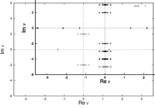
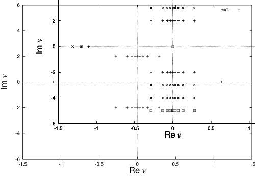
Figure 3: Location of zeros of $T^{(2)}_{n-1}(u,v)$ (upper) and $T^{(3)}_{n-1}(u,v)$ (lower) for $n=2,3,4,5$, $u=-0.1$, $p_{0}=5$, $N=20$. $T^{(2)}_{n-1}(u,v)$ has two real zeros for $n\leq 4$, which are absent for $n=5$. $T^{(3)}_{n-1}(u,v)$ has two real zeros for $n\leq 4$ and a double zero at $v=0$ for $n=5$. All the other zeros are located on an almost straight line $\Im v=\pm n\,\,\hbox{mod }2p_{0}$.

For example see Fig.3 showing the zeros of $T^{(2)}_{n-1}(u,v)$ for the case $p_{0}=5$, $u=-0.1$, $n=2,3,4,5$ and $N=20$. The main difference from the largest eigenvalue case is the presence of the two real zeros for $n<p_{0}$. Their absence for $n=p_{0}$ can be explained as follows. $T_{n-1}^{(2)}(u,v)$ in (3.4)–(3.6) is a Laurent polynomial of $e^{\frac{\theta}{2}v}$. When $m=N/2-1$, its highest/lowest terms are proportional to $\frac{\sin n\theta}{\sin\theta}e^{\pm\frac{N\theta}{2}v}$. This is vanishing when $n=p_{0}$, therefore the number of zeros decreases from $N$ to $N-2$. As a result $Y^{(2)}_{p_{0}-2}(v)$ tends to zero as $e^{-\theta|v|}$ for $v\rightarrow\pm\infty$.

As for the third largest eigenvalue we have the following for $u$ negative small (typically $u\sim-0.1$).

Conjecture 3

$T^{(3)}_{n-1}(u,v)$ has two real zeros $\pm\zeta^{(3)}_{n-1}$ for some $\zeta^{(3)}_{n-1}\in{\bf R}_{>0}$ for $n<p_{0}$ and a double zero at $\zeta^{(3)}_{p_{0}-1}=0$ for $n=p_{0}$. All the other zeros of $T^{(3)}_{n-1}(u,v)$ ($2\leq n\leq p_{0}$) are located on the almost straight lines $\Im v=\pm n\hbox{ mod }2p_{0}$.

See Fig.3 showing the zeros of $T^{(3)}_{n-1}(u,v)$ under the same conditions with $T^{(2)}_{n-1}(u,v)$. Again the main difference from the largest eigenvalue is the two additional zeros on the real axis.

When $v\to\pm\infty$, the $Y$-functions $Y^{(k)}_{j}$ and $K^{(k)}$ built from $T^{(k)}_{n-1}$ via (4.13)–(4.15) have the asymptotic values

$$Y^{(2)}_{j} \rightarrow \frac{\sin\frac{\pi(j+2)}{p_{0}}\sin\frac{\pi j}{p_{0}}}{\sin^{2}\frac{\pi}{p_{0}}},\quad Y^{(3)}_{j}\rightarrow j(j+2),$$ (6.1)

$$K^{(2)} \rightarrow -1,\quad\qquad\qquad\qquad K^{(3)}\rightarrow p_{0}-1.$$ (6.2)

To apply Lemma 1 to the $Y$-system (4.10)-(4.12), we modify the $Y$-functions as

$$\widetilde{Y}^{(k)}_{j}(v) = \frac{Y_{j}^{(k)}(v)}{F_{j}^{(k)}(v)}\quad\mbox{for}\,\,1\leq j\leq p_{0}-2,$$ (6.3)

$$\widetilde{K}^{(k)}(v) = \frac{K^{(k)}(v)}{\mbox{th}\frac{\pi}{4}(v+\zeta^{(k)}_{p_{0}-2})\mbox{th}\frac{\pi}{4}(v-\zeta^{(k)}_{p_{0}-2})},$$ (6.4)

where

$$F_{1}^{(k)}(v) = \{\mbox{th}\frac{\pi}{4}(v+i(1+u))\mbox{th}\frac{\pi}{4}(v-i(1+u))\}^{\frac{N}{2}}(\mbox{th}\frac{\pi}{4}v)^{2\delta_{k,3}}g^{(k)}(v)\quad\mbox{for}\,\,p_{0}=3,$$

$$F_{1}^{(k)}(v) = \mbox{th}\frac{\pi}{4}(v+\zeta^{(k)}_{2})\mbox{th}\frac{\pi}{4}(v-\zeta^{(k)}_{2})\{\mbox{th}\frac{\pi}{4}(v+i(1+u))\mbox{th}\frac{\pi}{4}(v-i(1+u))\}^{\frac{N}{2}}\quad\mbox{for}\,\,p_{0}\neq 3,$$

$$F_{j}^{(k)}(v) = \mbox{th}\frac{\pi}{4}(v+\zeta^{(k)}_{j+1})\mbox{th}\frac{\pi}{4}(v-\zeta^{(k)}_{j+1})\mbox{th}\frac{\pi}{4}(v+\zeta^{(k)}_{j-1})\mbox{th}\frac{\pi}{4}(v-\zeta^{(k)}_{j-1})\quad\mbox{for}\,\,2\leq j\leq p_{0}-3,$$

$$F_{p_{0}-2}^{(k)}(v) = \mbox{th}\frac{\pi}{4}(v+\zeta^{(k)}_{p_{0}-3})\mbox{th}\frac{\pi}{4}(v-\zeta^{(k)}_{p_{0}-3})(\mbox{th}\frac{\pi}{4}v)^{2\delta_{k,3}}g^{(k)}(v)\quad\mbox{for}\,\,p_{0}\neq 3.$$

The factor $g^{(k)}(v)$ defined by

$$g^{(k)}(v)=\cases{\exp\left(-\frac{\pi v}{p_{0}}\mbox{th}\frac{\pi}{4}v\right)&for $k=2$\cr 1&for $k=3$\cr}$$

has been included to compensate the singularity caused by $Y_{p_{0}-2}(v)$ tending to zero as $e^{-\frac{\pi}{p_{0}}|v|}$ at $v=\pm\infty$. The zeros $v=\zeta^{(k)}_{j}$ of $T^{(k)}_{j}(u_{N},v)$ depend on $N$ and converge to some finite values in the Trotter limit $N\to\infty$. By abuse of notation we shall also write their limit as $\zeta^{(k)}_{j}$. ($\zeta^{(3)}_{p_{0}-1}=0$ is valid irrespective of $N$.) Proceeding as in the free energy case, we get the non-linear integral equations obeyed by $\eta^{(k)}_{j}$ and $\kappa^{(k)}$:

$$\ln\eta^{(k)}_{1}(v) = -\frac{\beta\pi J\sin\theta}{2\theta\mbox{ch}(\frac{\pi v}{2})}+s_{1}\ast\ln\left((1+\kappa^{(k)})^{2}h^{(k)}\right)(v)+\delta_{k,2}\left(\pi i-\frac{\pi}{3}v\mbox{th}\frac{\pi v}{4}\right)$$ (6.5)

$$+2\delta_{k,3}\ln\mbox{th}\frac{\pi}{4}v\quad\mbox{for}\,\,p_{0}=3,$$

$$\ln\eta_{1}^{(k)}(v) = -\frac{\beta\pi J\sin\theta}{2\theta\mbox{ch}(\frac{\pi v}{2})}+s_{1}\ast\ln(1+\eta^{(k)}_{2})(v)+\ln\left\{\mbox{th}\frac{\pi}{4}(v+\zeta^{(k)}_{2})\mbox{th}\frac{\pi}{4}(v-\zeta^{(k)}_{2})\right\}\quad\mbox{for}\,\,p_{0}\neq 3,$$

$$\ln\eta^{(k)}_{j}(v) = s_{1}\ast\ln(1+\eta^{(k)}_{j-1})(1+\eta^{(k)}_{j+1})(v)+\ln\left\{\mbox{th}\frac{\pi}{4}(v+\zeta^{(k)}_{j+1})\mbox{th}\frac{\pi}{4}(v-\zeta^{(k)}_{j+1})\right\}$$ (6.7)

$$+\ln\left\{\mbox{th}\frac{\pi}{4}(v+\zeta^{(k)}_{j-1})\mbox{th}\frac{\pi}{4}(v-\zeta^{(k)}_{j-1})\right\}\quad\mbox{for}\,\,2\leq j\leq p_{0}-3,$$

$$\ln\eta^{(k)}_{p_{0}-2}(v) = s_{1}\ast\ln\left((1+\eta^{(k)}_{p_{0}-3})(1+\kappa^{(k)})^{2}h^{(k)}\right)(v)+\ln\left\{\mbox{th}\frac{\pi}{4}(v+\zeta^{(k)}_{p_{0}-3})\mbox{th}\frac{\pi}{4}(v-\zeta^{(k)}_{p_{0}-3})\right\}$$ (6.8)

$$+2\delta_{k,3}\ln\mbox{th}\frac{\pi}{4}v+\delta_{k,2}\left(\pi i-\frac{\pi}{p_{0}}v\mbox{th}\frac{\pi v}{4}\right)\quad\mbox{for}\,\,p_{0}\neq 3,$$

$$\ln\kappa^{(k)}(v) = s_{1}\ast\ln(1+\eta^{(k)}_{p_{0}-2})(v)+\ln\left\{\mbox{th}\frac{\pi}{4}(v+\zeta^{(k)}_{p_{0}-2})\mbox{th}\frac{\pi}{4}(v-\zeta^{(k)}_{p_{0}-2})\right\}+\delta_{k,2}\pi i,$$ (6.9)

where

$$h^{(k)}(v)=\cases{\exp\left(\frac{2\pi}{p_{0}}\left(v\mbox{th}\frac{\pi v}{2}-\frac{1}{\mbox{ch}\frac{\pi v}{2}}\right)\right)&for $k=2$\cr 1&for $k=3$\cr}.$$

Here the integration constants have been fixed from the asymptotic values (6.1) and (6.2). In addition to these we need to impose the consistency condition coming from $T^{(k)}_{j}(\zeta^{(k)}_{j})=0$, which determines the real zeros $\{\pm\zeta^{(k)}_{j}\,|\,\zeta^{(k)}_{j}>0,k=2,3,j\in\{1,\cdots,p_{0}-2\}\}$. ($\zeta^{(3)}_{p_{0}-1}=0$.) From (4.14) and (5.5) this leads to setting $\eta^{(k)}_{j}(\zeta_{j}^{(k)}\pm i)=-1$ in (6.5)–(6.8). Explicitly they read

for $$p_{0}=3,$$

$$i\frac{\beta\pi J\sin\theta}{2\theta\mbox{sh}(\frac{\pi\zeta^{(k)}_{1}}{2})}+s_{1}\ast\ln\left((1+\kappa^{(k)})^{2}h^{(k)}\right)(\zeta^{(k)}_{1}+i)-\delta_{k,2}\frac{\pi}{3}(\zeta^{(k)}_{1}+i)\mbox{th}\frac{\pi(\zeta^{(k)}_{1}+i)}{4}$$

$$+\delta_{k,3}\left\{\pi i+\ln\left(\frac{\mbox{sh}(\frac{\pi}{2}\zeta^{(3)}_{1})+i}{\mbox{sh}(\frac{\pi}{2}\zeta^{(3)}_{1})-i}\right)\right\}=0,$$

for $$p_{0}\neq 3,$$

$$i\frac{\beta\pi J\sin\theta}{2\theta\mbox{sh}(\frac{\pi\zeta^{(k)}_{1}}{2})}+s_{1}\ast\ln(1+\eta^{(k)}_{2})(\zeta_{1}^{(k)}+i)+\ln\left(\frac{\mbox{sh}(\frac{\pi}{2}\zeta^{(k)}_{1})+i\mbox{ch}(\frac{\pi}{2}\zeta^{(k)}_{2})}{\mbox{sh}(\frac{\pi}{2}\zeta^{(k)}_{1})-i\mbox{ch}(\frac{\pi}{2}\zeta^{(k)}_{2})}\right)+\pi i=0,$$

for $$2\leq j\leq p_{0}-3,$$

$$s_{1}\ast\ln(1+\eta^{(k)}_{j-1})(1+\eta^{(k)}_{j+1})(\zeta^{(k)}_{j}+i)$$

$$+\ln\left(\frac{\mbox{sh}(\frac{\pi}{2}\zeta^{(k)}_{j})+i\mbox{ch}(\frac{\pi}{2}\zeta^{(k)}_{j+1})}{\mbox{sh}(\frac{\pi}{2}\zeta^{(k)}_{j})-i\mbox{ch}(\frac{\pi}{2}\zeta^{(k)}_{j+1})}\right)+\ln\left(\frac{\mbox{sh}(\frac{\pi}{2}\zeta^{(k)}_{j})+i\mbox{ch}(\frac{\pi}{2}\zeta^{(k)}_{j-1})}{\mbox{sh}(\frac{\pi}{2}\zeta^{(k)}_{j})-i\mbox{ch}(\frac{\pi}{2}\zeta^{(k)}_{j-1})}\right)+\pi i=0,$$

for $$p_{0}\neq 3,$$

$$s_{1}\ast\ln\left((1+\eta^{(k)}_{p_{0}-3})(1+\kappa^{(k)})^{2}h^{(k)}\right)(\zeta^{(k)}_{p_{0}-2}+i)+\ln\left(\frac{\mbox{sh}(\frac{\pi}{2}\zeta^{(k)}_{p_{0}-2})+i\mbox{ch}(\frac{\pi}{2}\zeta^{(k)}_{p_{0}-3})}{\mbox{sh}(\frac{\pi}{2}\zeta^{(k)}_{p_{0}-2})-i\mbox{ch}(\frac{\pi}{2}\zeta^{(k)}_{p_{0}-3})}\right)$$

$$+\delta_{k,3}\left\{\pi i+\ln\left(\frac{\mbox{sh}(\frac{\pi}{2}\zeta^{(k)}_{p_{0}-2})+i}{\mbox{sh}(\frac{\pi}{2}\zeta^{(k)}_{p_{0}-2})-i}\right)\right\}-\delta_{k,2}\frac{\pi}{p_{0}}(\zeta^{(2)}_{p_{0}-2}+i)\mbox{th}\frac{\pi(\zeta^{(2)}_{p_{0}-2}+i)}{4}=0,$$

where the convolutions should be interpreted as

$$s_{1}*g(\zeta+i)=\mbox{p.v.}\left(\int^{\infty}_{-\infty}\frac{g(x)}{4i\mbox{sh}\frac{\pi}{2}(\zeta-x)}dx\right)+\frac{1}{2}g(\zeta).$$

Here p.v. means the principal value. Since $T^{(k)}_{1}(u_{N},0)$ is negative from the numerical experiment, $\lim_{N\to\infty}|T^{(k)}_{1}(u_{N},0)|$ can be expressed as

$$\lim_{N\to\infty}|T^{(k)}_{1}(u_{N},0)| = -\frac{J}{2}\beta\cos\theta+\int^{\infty}_{-\infty}dvs_{1}(v)\ln(1+\eta^{(k)}_{1}(v))$$ (6.14)

$$+\frac{2\pi J\sin\theta}{\theta}\beta\int^{\infty}_{-\infty}dva_{1}(v)s_{1}(v)+2\ln\mbox{th}\frac{\pi}{4}\zeta^{(k)}_{1}.$$

Finally we obtain the correlation length (2.13) as

$$\frac{1}{\xi_{k}}=-2\ln\mbox{th}\frac{\pi}{4}\zeta^{(k)}_{1}-\int^{\infty}_{-\infty}dvs_{1}(v)\ln\left(\frac{1+\eta^{(k)}_{1}(v)}{1+\eta^{(1)}_{1}(v)}\right).$$ (6.15)

We can solve (6.5)–(LABEL:z2) numerically as follows. First we solve the BAE (3.7) numerically for a finite $N$ and determine the $Y$-functions and their real zeros. This serves as the first approximation of their large $N$ limit $\eta^{(k)}_{j}$ and $\kappa^{(k)}$. Second we input them into the rhs of (6.5)-(6.9) and get the new $\eta$-functions in the lhs as an output. Third we substitute the output $\eta$-functions into (6)-(LABEL:z2). Solving them by Newton’s method a new output for the zeros $\zeta^{(k)}_{j}$ can also be constructed. Finally by iterating the second and the third processes in the above until adequate convergence is achieved, the $\eta$-functions and their real zeros are determined accurately. In this way the present approach enables us to overcome the difficulty of the naive numerical extrapolation of $T^{(k)}_{1}$ as $N\rightarrow\infty$ mentioned in the introduction.

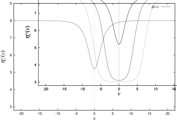
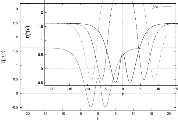
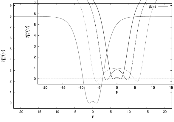
Figure 4: The function $\eta^{(k)}_{2}(v)$ for $v$ real, $p_{0}=5$ and $k=1,2,3$.

For a comparison we depict the functions $\eta^{(k)}_{2}(v)\,(k=1,2,3)$ in Fig.4 under the same parameters. We also include the graphs of the correlation lengths $\xi_{2}$ and $\xi_{3}$ for $p_{0}=2,3,4,5$ in Fig.5. In the low temperature limit these results agree with the earlier ones in [12, 25].

$$\lim_{\beta\to\infty}\xi_{2}(\beta)/\beta = \frac{J\pi\sin\theta}{2(\pi-\theta)\theta},$$ (6.16)

$$\lim_{\beta\to\infty}\xi_{3}(\beta)/\beta = \frac{J(\pi-\theta)\sin\theta}{2\pi\theta}$$ (6.17)

with high accuracy.

7 Summary and discussion

We have revisited the thermodynamics of the spin $\frac{1}{2}$ XXZ model at roots of unity by the QTM method. Functional relations indexed by the TS numbers are found among the fusion hierarchy of QTM’s ($T$-system) and their certain ratios ($Y$-system). As a peculiar feature of a general root of unity, the $Y$-functions (4.3)–(4.5) and the $Y$-system (4.9)–(4.9) are considerably involved compared with those in [29]. Nevertheless they have a nice analyticity allowing a transformation to integral equations. Our approach simplifies the numerics to examine the analyticity drastically in that only the largest eigenvalue sector of the QTM $T_{1}$ is needed for the free energy. We have set up Conjecture 1 on the zeros of QTM’s supported by an extensive numerical study. The resulting integral equations exactly coincide with the TBA equation in [18] based on the string hypothesis. Another and more significant advantage of the present method is to allow us to study correlation lengths on an equal footing with the free energy by considering other eigensectors of $T_{1}$. The additional zeros and poles coming into the ANZC strips play a fundamental role in characterizing the relevant excited states. We have considered the second and the third largest eigenvalues of $T_{1}$, which are related to the spin–spin correlation lengths for $\langle\sigma_{j}^{+}\sigma_{i}^{-}\rangle$ and $\langle\sigma_{j}^{z}\sigma_{i}^{z}\rangle$, respectively. The excited state TBA equation is derived and numerically solved to evaluate the correlation lengths. The result shows a good agreement with the earlier one in the low temperature limit.

Let us remark a few straightforward generalizations of the present results. (1) the XYZ model, (2) higher spin cases and (3) inclusion of external field $h$. For (1) and (2), the $T$ and $Y$-systems remain essentially the same. We have an additional periodicity in the real direction in the complex $v$-plane for (1). This does not complicate actual calculations too much. In (2) the driving term will enter the TBA equation in a different manner from (5.7)-(5.9). As noted in [35], the commensurability between the magnitude of the spin and the anisotropy parameter would be of issue. This is also an interesting problem in view of the present approach. For case (3) the BAE (3.7) should be modified with an extra $\exp(2\beta h)$ factor in the rhs. Consequently, the BAE roots for the largest eigenvalue will distribute away from the real axis. This is a significant difference from the usual row-to-row case where they remain on the real axis even for $h\neq 0$. The numerical check of the ANZC property therefore needs more elaboration. The $T$-system (4.2) also needs to be modified into

$$T_{y_{\alpha+y_{\alpha-1}-1}}(v)=T_{y_{\alpha}-y_{\alpha-1}-1}(v)+2(-1)^{mz_{\alpha}}\mbox{ch}(\beta hy_{\alpha})T_{y_{\alpha-1}-1}(v+iy_{\alpha}).$$

Correspondingly, (4.9) is replaced by

$$Y_{m_{\alpha}-1}(v)=K(v)^{2}+2\mbox{ch}(\beta hy_{\alpha})K(v).$$

These modifications are consistent with [18] from the string hypothesis. Explicit evaluation of the effects of the magnetic field on correlation lengths will be an interesting problem manageable within the present scheme.

Acknowledgements. A. K. thanks M. T. Batchelor, E. A. and R. J. Baxter and V. V. Bazhanov for hospitality at International workshop on statistical mechanics and integrable systems, July 20 – August 8, 1997 held in Coolangatta and Canberra, where part of this work was presented. He also thanks A. Berkovich, B. M. McCoy and A. Schilling for comments. A. K. and K. S. are grateful to M. Takahashi for useful discussions.

Appendix A   Takahashi-Suzuki (TS) numbers

Given $\{\nu_{j}\}$ in the continued fraction expansion (4.1) we define the sequences of numbers $\{m_{j}\}_{j=0}^{\alpha+1},\{p_{j}\}_{j=0}^{\alpha+1},\{y_{j}\}_{j=-1}^{\alpha},\{z_{j}\}_{j=-1}^{\alpha},\{n_{j}\}_{j\geq 1},\{\widetilde{n}_{j}\}_{j\geq 1}$ and $\{w_{j}\}_{j\geq 1}$ as follows. The sequence $\{m_{j}\}_{j=0}^{\alpha+1}$ is define by

$$m_{j}=\nu_{1}+\nu_{2}+\cdots+\nu_{j}\quad 0\leq j\leq\alpha,$$ (A.1)

$$m_{\alpha+1}=\infty.$$

The sequence $\{p_{j}\}_{j=0}^{\alpha+1}$ is defined by

$$p_{j}=p_{j-2}-\nu_{j-1}p_{j-1}\quad 2\leq j\leq\alpha+1,$$

$$p_{0}=\frac{\pi}{\theta},\,p_{1}=1,p_{2}=p_{0}-\nu_{1}.$$

It can be easily shown that

$$p_{\alpha+1}=0,$$ (A.2)

$$p_{j}<\frac{p_{j-1}}{\nu_{j}},\,p_{j}<\frac{p_{0}}{2}\quad\mbox{if }1\leq j\leq\alpha+1,$$ (A.3)

$$2p_{j}+2p_{j+1}<p_{0}\quad\mbox{if }2\leq j\leq\alpha\hbox{ or }j=1,\nu_{1}\geq 3.$$ (A.4)

The sequences $\{y_{j}\}_{j=-1}^{\alpha}$ and $\{z_{j}\}_{j=-1}^{\alpha}$ are defined by

$$y_{j}=y_{j-2}+\nu_{j}y_{j-1}\quad 1\leq j\leq\alpha,$$

$$y_{-1}=0,y_{0}=1,y_{1}=\nu_{1},y_{2}=1+\nu_{1}\nu_{2},$$ (A.5)

$$z_{j}=z_{j-2}+\nu_{j}z_{j-1}\quad 1\leq j\leq\alpha,$$

$$z_{-1}=1,z_{0}=0,z_{1}=1,z_{2}=\nu_{2}.$$ (A.6)

Obviously, $z_{j}=y_{j-1}|_{\nu_{k}\rightarrow\nu_{k+1}}$ and they are all positive integers except $y_{-1}=z_{0}=0$. By induction one can verify

$$y_{j}=z_{j}p_{0}+(-1)^{j}p_{j+1}\quad-1\leq j\leq\alpha,$$ (A.7)

$$y_{\alpha}=z_{\alpha}p_{0},$$ (A.8)

where the latter is a consequence of the former with $j=\alpha$ and (A.2). In fact $GCD(y_{\alpha},z_{\alpha})=1$ is valid. Now we introduce the Takahashi-Suzuki (TS) numbers $\{n_{j}\}_{j\geq 1}$ [18] and their slight rearrangement $\{{\widetilde{n}_{j}}\}_{j\geq 1}$ by

$$n_{j}=y_{r-1}+(j-m_{r})y_{r}\quad m_{r}\leq j<m_{r+1},$$ (A.9)

$${\widetilde{n}}_{j}=y_{r-1}+(j-m_{r})y_{r}\quad m_{r}<j\leq m_{r+1}.$$ (A.10)

Obviously, ${\widetilde{n}}_{j}=n_{j}$ except ${\widetilde{n}}_{m_{r}}=y_{r}$ while $n_{m_{r}}=y_{r-1}$. In particular, there is a duplication $n_{1}=n_{m_{1}}=1$, while the modified sequence ${\widetilde{n}}_{j}$ is strictly increasing with $j$. In this paper we are concerned with the first $m_{\alpha}+1$ of them. As the set with multiplicity

$$\{{\widetilde{n}}_{j}\}_{j=1}^{m_{\alpha}+1}=\{n_{j}\}_{j=1}^{m_{\alpha}+1}\sqcup\{y_{\alpha}\}\setminus\{1\}.$$

We note that if $p_{0}\geq 2$ we always have ${\tilde{n}}_{j}=j$ for $j=1,2$ and 3. In parallel with (A.5) and (A.6) we consider the “$z$-analogue” $\{w_{j}\}_{j\geq 1}$ of $\{n_{j}\}_{j\geq 1}$:

$$w_{j}=z_{r-1}+(j-m_{r})z_{r}-1\quad m_{r}\leq j<m_{r+1}.$$

For example, $w_{1}=w_{m_{2}}=0$ and $w_{m_{1}}=-1$. It is possible to show

$$\left[\frac{n_{j}-1}{p_{0}}\right]=w_{j}+\delta_{jm_{1}}\quad 1\leq j\leq m_{\alpha},$$ (A.11)

where $[x]$ denotes the largest integer not exceeding $x$. As a result the sequence $\{w_{j}\}$ is related to the parity $v_{j}$ in (2.14) of [18] by $v_{j}=(-1)^{w_{j}}$ for all $1\leq j\leq m_{\alpha}$. Using (A.7), (A.10) and (Appendix A   Takahashi-Suzuki (TS) numbers) one can show

$$\{w_{j}p_{0}\pm{\tilde{n}}_{j+1}\pm y_{r}\hbox{ mod }2p_{0}\}=\{p_{0}\pm(p_{r}-(j+1\pm 1-m_{r})p_{r+1})\hbox{ mod }2p_{0}\}$$ (A.12)

for $m_{r}\leq j<m_{r+1}$. Here the signs $\pm$ are independent.

It is well known [18, 35, 36] that for the TS numbers $n_{j}$, the equivalent conditions

$$(-1)^{w_{j}}\sin\left(\frac{\pi k}{p_{0}}\right)\sin\left(\frac{\pi(n_{j}-k)}{p_{0}}\right)>0,$$ (A.13)

$$\left[\frac{k}{p_{0}}\right]+\left[\frac{n_{j}-k}{p_{0}}\right]=\left[\frac{n_{j}-1}{p_{0}}\right],$$ (A.14)

hold for $k=1,2,\ldots,n_{j}-1$. It is interesting to observe the condition (A.13) in the light of the associated fusion transfer matrix $T_{n_{j}-1}(u,v)$ (3.1). From (3) and (2.5), we see that (A.13) ensures that $\epsilon_{jj^{\prime}}$ and $\epsilon^{\prime}_{jj^{\prime}}$ can be independent of their indices for the constituent fusion Boltzmann weights to be real.

Appendix B   ANZC property of $Y_{j}^{(1)}(v)$

Let us check the applicability of Lemma 1 in section 5 to the $Y$-system (4.9)–(4.9) by admitting Conjecture 1. Apart from the exceptional Case 1, 2 and 3 listed there, we are to verify that $Y^{(1)}_{j}(v)$, for example, is ANZC in the strip ${\cal S}[x]$ whenever the combination $Y^{(1)}_{j}(v+ix)Y^{(1)}_{j}(v-ix)$ takes place. Case 1 has been argued in section 5 and Case 2 and 3 will be considered in Appendix C.

Conjecture 1 tells that the zeros and poles of the $Y$-functions (4.3)–(4.5) are located as

$$Y^{(1)}_{j}(v),1+Y^{(1)}_{j}(v): \Im v\sim w_{j}p_{0}\pm\widetilde{n}_{j+1}\pm y_{r}\quad 1\leq j\leq m_{\alpha}-1,$$

$$K^{(1)}(v): \Im v\sim w_{m_{\alpha}-1}p_{0}\pm y_{\alpha-1}+y_{\alpha}.$$

Here the signs $\pm$ are independent and we have taken the periodicity under $v\rightarrow v+2p_{0}i$ into account. See (3.8). From (A.12) these functions are ANZC in the following strips:

For $$m_{r}\leq j\leq m_{r+1}-2\,\,(0\leq r\leq\alpha-1),$$ (B.3)

$$Y^{(1)}_{j}(v),1+Y^{(1)}_{j}(v):\,\,{\cal S}[p_{0}-p_{r}+(j-m_{r})p_{r+1}-\delta],$$

$$Y^{(1)}_{m_{r}-1}(v),1+Y^{(1)}_{m_{r}-1}(v):\,\,{\cal S}[p_{0}-p_{r}-p_{r+1}-\delta],$$

$$1+Y^{(1)}_{m_{\alpha}-1}(v),1+K^{(1)}(v),K^{(1)}(v):\,\,{\cal S}[p_{0}-p_{\alpha}-\delta].$$

In the above $\delta$ denotes a small real number $(|\delta|\sim 10^{-2})$ caused by the deviations of the actual zeros of $T^{(1)}_{n-1}(v)$ from the straight line specified in Conjecture 1. They of course depend on the $Y$-functions but have been denoted by the same symbol for the sake of simplicity. On the other hand, Lemma 1 is applicable to the $Y$-system (4.9)–(4.9) if the $Y$-functions are ANZC in the strips:

$$Y^{(1)}_{j}(v):\,\,{\cal S}[p_{r+1}]\,\,(m_{r}\leq j\leq m_{r+1}-2,\,0\leq r\leq\alpha-1),$$ (B.4)

$$Y^{(1)}_{m_{r}-1}(v):\,\,{\cal S}[p_{r}+p_{r+1}]\,(1\leq r\leq\alpha-1),$$ (B.5)

$$1+Y^{(1)}_{m_{r}-1}(v):\,\,{\cal S}[p_{r}-p_{r+1}]\,(1\leq r\leq\alpha-1),$$ (B.6)

$$1+Y^{(1)}_{m_{r}-2}(v):\,\,{\cal S}[p_{r+1}]\,(1\leq r\leq\alpha-1),$$ (B.7)

$$1+Y^{(1)}_{m_{r}}(v):\,\,{\cal S}[p_{r}]\,(1\leq r\leq\alpha-1),$$ (B.8)

$$K^{(1)}(v):\,\,{\cal S}[p_{\alpha}],$$ (B.9)

$$1+K^{(1)}(v),\{1+Y^{(1)}_{j}(v)\}_{j=1}^{m_{\alpha}-1}\hbox{ other than (\ref{anzc10})--(\ref{anzc12})}:\,\,{\cal S}[0^{+}],$$ (B.10)

where ${\cal S}[0^{+}]$ means the vicinity along the real axis which can be arbitrarily thin. If $\nu_{1}=2$, the $r=1$ case of (B.7) is void.

Except for Cases 1, 2 and 3 in section 5, it is straightforward to verify that the strips in (B.4)–(B.10) are narrower than those in (B.3)–(B.3) for the corresponding functions. As an illustration we prove here that ${\cal S}[p_{0}-p_{r}+(j-m_{r})p_{r+1}-\delta]\supset{\cal S}[p_{r+1}]$ for the strips in (B.3) and (B.4). The rest is a similar exercise. We only have to show the inequality

$$p_{0}-p_{r}+(j-m_{r})p_{r+1}-\delta>p_{r+1}\quad\hbox{for}\,\,m_{r}\leq j\leq m_{r+1}-2.$$ (B.11)

Though this is incorrect for $j=1$ (hence $r=0$), this case corresponds to Case 1, for which the difficulty has been cleared in section 5 by a modification of a $Y$-function. Now suppose $j\neq 1$. It is enough to check (B.11) only for $j=m_{r}\,\,(r\geq 1)$. Making use of the properties in (A.3) one has

$$p_{0}-p_{r+1}-p_{r}-\delta\geq p_{0}-p_{2}-p_{1}-\delta=\nu_{1}-1-\delta.$$ (B.12)

By noting that $\nu_{1}\geq 2$ and $|\delta|\ll 1$, the last quantity is non-negative, proving (B.11).

Appendix C   ANZC property of $Y^{(1)}_{j}(v)$ for exceptional cases

Let us show that Lemma 1 can still be applied to the $Y$-system in Case 2 and 3 in section 5 after suitable recombinations of the $Y$-functions. For a function whose logarithmic derivative can be Fourier transformed we use the notation

$${\cal F}[f](k)=\frac{1}{2\pi}\int_{-\infty}^{\infty}\frac{d}{dv}\ln f(v)e^{-ikv}dv.$$

We start with Case 2. Explicitly it reads

$$Y^{(1)}_{2}(v-i(4-p_{0}))Y^{(1)}_{2}(v+i(4-p_{0}))Y^{(1)}_{2}(v-i(p_{0}-2))Y^{(1)}_{2}(v+i(p_{0}-2))=$$

$$(1+Y^{(1)}_{1}(v+i(p_{0}-3)))(1+Y^{(1)}_{1}(v-i(p_{0}-3)))(1+Y^{(1)}_{2}(v+i(4-p_{0})))$$

$$\times(1+Y^{(1)}_{2}(v-i(4-p_{0})))(1+Y^{(1)}_{3}(v+i))(1+Y^{(1)}_{3}(v-i)),$$ (C.1)

where

$$1+Y^{(1)}_{3}(v)=\frac{T^{(1)}_{3}(v+i(p_{0}-3))T^{(1)}_{3}(v-i(p_{0}-3))}{T^{(1)}_{2}(v+i(4-p_{0}))T^{(1)}_{2}(v-i(4-p_{0}))},$$ (C.2)

and the other functions are given by (4.13) and (4.14). From the Case 2 conditions on $\nu_{1}$–$\nu_{3}$, we have $p_{0}=4-\epsilon$ with $0<\epsilon\ll 1$. Thus the ANZC argument can not be applied to some factors in (C.1). For example the $Y^{(1)}_{2}(v)$-function in the lhs has zeros or poles along $\Im v\simeq 2$. They are outside of ${\cal S}[4-p_{0}]$ but can be within ${\cal S}[p_{0}-2]$. Similarly zeros of the $1+Y^{(1)}_{1}(v)$ in the rhs lie along $\Im v\simeq 1$ which is in the strip ${\cal S}[p_{0}-3]$. A recipe here is to consider the combination

$$X(v)=\frac{Y^{(1)}_{2}(v+i)Y^{(1)}_{2}(v-i)}{1+Y^{(1)}_{1}(v)}=\frac{T^{(1)}_{3}(v+i)T^{(1)}_{3}(v-i)}{T_{0}(v+4i)T_{0}(v-4i)},$$ (C.3)

which is ANZC in ${\cal S}[p_{0}-3]$. With this, (C.1) can be rewritten as

$$X(v+i(p_{0}-3))X(v-i(p_{0}-3))$$

$$=(1+Y^{(1)}_{2}(v+i(p_{0}-4)))(1+Y^{(1)}_{2}(v-i(p_{0}-4)))(1+Y^{(1)}_{3}(v+i))$$

$$\times(1+Y^{(1)}_{3}(v-i)).$$ (C.4)

At this stage, the lemma applies to both (C.3) and (C.4) giving

$${\cal F}[X](k) = 2\mbox{ch}k{\cal F}[Y^{(1)}_{2}](k)-{\cal F}[1+Y^{(1)}_{1}](k),$$

$${\cal F}[X](k) = \frac{\mbox{ch}(4-p_{0})k}{\mbox{ch}(p_{0}-3)k}{\cal F}[1+Y^{(1)}_{2}](k)$$

$$+ \frac{\mbox{ch}k}{\mbox{ch}(p_{0}-3)k}{\cal F}[1+Y^{(1)}_{3}](k).$$

Eliminating ${\cal F}[X](k)$ from these and doing the inverse Fourier transformation, we get (5.8).

Next we consider Case 3.

$$Y^{(1)}_{1}(v+i(1-p_{2}))Y^{(1)}_{1}(v-i(1-p_{2}))Y^{(1)}_{1}(v+i(1+p_{2}))Y^{(1)}_{1}(v-i(1+p_{2}))$$

$$=(1+Y^{(1)}_{2}(v+i))(1+Y^{(1)}_{2}(v-i))(1+Y^{(1)}_{1}(v+i(3-p_{0})))$$

$$\times(1+Y^{(1)}_{1}(v-i(3-p_{0}))),$$ (C.5)

where

$$1+Y^{(1)}_{2}(v) = \frac{T^{(1)}_{2}(v+i(p_{0}-2))T^{(1)}_{2}(v-i(p_{0}-2))}{T_{0}(v+i(3-p_{0}))T_{0}(v-i(3-p_{0}))},$$ (C.6)

and the other functions are given by (4.13) and (4.14). Now $p_{0}=2+p_{2}$. $Y^{(1)}_{1}(v)$ has zeros (resp. poles) at $v=\pm(1+u)i$ (resp. $v=\pm(1-u)i$) $\in{\cal S}[1+p_{2}]$, which prevents the direct application of Lemma 1 in the last two factors in the lhs of (C.5) for $J>0$ (resp. $J<0$). This can be remedied by introducing $\widetilde{Y}^{(1)}_{1}(v)=Y^{(1)}_{1}(v)/(\mbox{th}(\frac{\pi}{4}\frac{v-i(1\pm u)}{1+p_{2}})\mbox{th}(\frac{\pi}{4}\frac{v+i(1\pm u)}{1+p_{2}}))^{\pm N/2}$ as in section 5. In the rhs of (C.5), there are also some factors possessing zeros or poles and making Lemma 1 inapplicable. However the new combinations

$$G_{1}(v) = (1+Y^{(1)}_{2}(v))(1+Y^{(1)}_{1}(v-i(p_{0}-2)))$$

$$= \frac{T^{(1)}_{2}(v+i(p_{0}-2))}{T^{(1)}_{1}(v-i(3-p_{0}))}\frac{T^{(1)}_{2}(v-i(p_{0}-2))}{T_{0}(v+i(4-p_{0}))}\frac{T^{(1)}_{1}(v-i(p_{0}-1))}{T_{0}(v-ip_{0})},$$

$$G_{2}(v) = (1+Y^{(1)}_{2}(v))(1+Y^{(1)}_{1}(v+i(p_{0}-2)))$$

$$= \frac{T^{(1)}_{2}(v+i(p_{0}-2))}{T^{(1)}_{1}(v+i(3-p_{0}))}\frac{T^{(1)}_{2}(v-i(p_{0}-2))}{T_{0}(v-i(4-p_{0}))}\frac{T^{(1)}_{1}(v+i(p_{0}-1))}{T_{0}(v+ip_{0})}$$

are free of these spurious zeros and poles and ANZC in $\Im v\in[0,1]$ and $[-1,0]$, respectively. With their aid (C.5) can be written as

$$Y^{(1)}_{1}(v+i(1-p_{2}))Y^{(1)}_{1}(v-i(1-p_{2}))\widetilde{Y}^{(1)}_{1}(v+i(1+p_{2}))\widetilde{Y}^{(1)}_{1}(v-i(1+p_{2}))$$

$$=G_{1}(v+i)G_{2}(v-i).$$

Solving these relations as in Case 2, we obtain the solution in Fourier space,

$${\cal F}[Y^{(1)}_{1}](k) = \frac{iN\mbox{sh}ku}{2\mbox{ch}k}$$

$$+ \frac{\mbox{ch}(p_{0}-3)k}{2\mbox{ch}p_{2}k\mbox{ch}k}{\cal F}[1+Y^{(1)}_{1}](k)+\frac{1}{2\mbox{ch}p_{2}k}{\cal F}[1+Y^{(1)}_{2}](k),$$

which can be transformed back to (5.8).

Appendix D   Free fermion case

Here we consider the free energy and the correlation lengths for the free fermion case $\Delta=0$ ($p_{0}=2,\alpha=1$) in (2.1). In this case we have $\phi(v+4i)=(-1)^{\frac{N}{2}}\phi(v)$ and $Q(v+4i)=(-1)^{m}Q(v)$ from (3.5) and (3.6). Thus (3.4) simplifies to

$$T_{1}(v)=\varrho(v)\frac{Q(v+2i)}{Q(v)},$$ (D.1)

where

$$\varrho(u,v)=\phi\bigl{(}v-i(u+2)\bigr{)}\phi(v+iu)+(-1)^{m}\phi\bigl{(}v+i(u+2)\bigr{)}\phi(v-iu).$$

One can directly show $T_{1}(v+i)T_{1}(v-i)=(-1)^{m}\varrho(v+i)\varrho(v-i)$. This rhs is a known function, which is a distinct feature of the free fermion model. We find it convenient to introduce

$$\widetilde{T}^{(k)}_{1}(u,v) = \frac{T_{1}^{(k)}(u,v)}{\phi(v+i(u+2))\phi(v-i(u+2))}$$

$$= \left(\frac{\phi(v+iu)}{\phi(v+i(u+2))}+(-1)^{m}\frac{\phi(v-iu)}{\phi(v-i(u+2))}\right)\frac{Q(v+2i)}{Q(v)}.$$

It satisfies

$$\widetilde{T}_{1}^{(k)}(u,v+i)\widetilde{T}_{1}^{(k)}(u,v-i)=(X(u,v)^{\frac{1}{2}}+(-1)^{\frac{N}{2}-m}X(u,v)^{-\frac{1}{2}})^{2},$$ (D.2)

where

$$X(u,v)=\frac{\phi(v+i(u-1))\phi(v-i(u-1))}{\phi(v+i(u+1))\phi(v-i(u+1))}.$$

First we consider the free energy characterized by the largest eigenvalue $T_{1}^{(1)}(u,v)$. It lies in the sector $m=N/2$. Since the function $\widetilde{T}^{(1)}_{1}(u,v)$ is ANZC for $v\in{\cal S}[1]$, we have

$$2\mbox{ch}k\,{\cal F}[\widetilde{T}^{(1)}_{1}](k)=2{\cal F}\,[X^{\frac{1}{2}}+X^{-\frac{1}{2}}](k).$$ (D.3)

See Appendix C for the notation ${\cal F}$. By the inverse Fourier transformation and the identity

$$\int_{-\infty}^{\infty}\frac{e^{-ikv}}{2\mbox{ch}k}dk=\frac{\pi}{2\mbox{ch}\frac{\pi v}{2}}=2\pi s_{1}(v),$$

we get

$$\ln\widetilde{T}^{(1)}_{1}(u,v)=2\left[s_{1}\ast\ln(X^{\frac{1}{2}}+X^{-\frac{1}{2}})\right](v).$$ (D.4)

See (5.10). Using the relations

$$\lim_{N\to\infty}X(u_{N},v)=\exp\left(\frac{J\beta}{\mbox{ch}\frac{\pi v}{2}}\right),\quad\lim_{N\to\infty}\widetilde{T}^{(k)}_{1}(u_{N},0)=\lim_{N\to\infty}T^{(k)}_{1}(u_{N},0),$$

we obtain the free energy per site $f$ as

$$f = -\frac{1}{\beta}\lim_{N\rightarrow\infty}\ln T^{(1)}_{1}(u_{N},0)$$ (D.5)

$$= -\frac{2}{\pi\beta}\int_{0}^{\frac{\pi}{2}}\ln\left(2\mbox{ch}(\frac{J\beta}{2}\cos\eta)\right)d\eta$$

in agreement with [37].

Next we consider the correlation length $\xi_{2}$ for $\langle\sigma_{j}^{+}\sigma_{i}^{-}\rangle$ which is related to the second largest eigenvalue $T_{1}^{(2)}(v)$. This lies in the sector $m=N/2-1$. From a numerical check, $T_{1}^{(2)}(u,v)$ is ANZC for $v\in{\cal S}[1]$. Therefore we can calculate it in the same way as $T_{1}^{(1)}(u,v)$ The only difference is

$$\ln\widetilde{T}^{(2)}_{1}(v)=2[s_{1}\ast\ln(X^{\frac{1}{2}}-X^{-\frac{1}{2}})](v)$$ (D.6)

due to (D.2) with $m=N/2-1$. Thus we have

$$\lim_{N\to\infty}\ln|T_{1}^{(2)}(u_{N},0)|=\frac{2}{\pi}\int_{0}^{\frac{\pi}{2}}\ln\left(2\mbox{sh}(\frac{|J\beta|}{2}\cos\eta)\right)d\eta.$$

Combining this with (D.5) and (2.13) we find the $\xi_{2}$ for $\langle\sigma_{j}^{+}\sigma_{i}^{-}\rangle$:

$$\frac{1}{\xi_{2}}=-\frac{2}{\pi}\int_{0}^{\frac{\pi}{2}}\ln\left(2\mbox{th}(\frac{|J\beta|}{2}\cos\eta)\right)d\eta.$$ (D.7)

This result coincides with those in [4], [37]–[39].

Finally we consider the correlation length $\xi_{3}$ for $\langle\sigma_{j}^{z}\sigma_{i}^{z}\rangle$ characterized by the third largest eigenvalue $T_{1}^{(3)}(u,v)$. This lies in the sector $m=N/2$, which is the same with $T_{1}^{(1)}(u,v)$. All the BAE roots for $T_{1}^{(1)}(u,v)$ are real solutions of $\varrho(v)=0$. The set of the BAE roots for $T_{1}^{(3)}(u,v)$ is the same with the one for $T_{1}^{(1)}(u,v)$ except that the largest magnitude ones $\pm\zeta$ are replaced by 0 and $2i$. It follows from (D.1) that $T^{(3)}_{1}(u,v)=T^{(1)}_{1}(u,v)\mbox{th}\frac{\pi}{4}(v+\zeta)\mbox{th}\frac{\pi}{4}(v-\zeta)$. In the Trotter limit, the real zeros $\pm\zeta$ are the largest magnitude solutions to $\varrho(u_{N},v)|_{N\to\infty}=0$ given by

$$\zeta=\frac{2}{\pi}\mbox{sh}^{-1}\left(\frac{J\beta}{\pi}\right).$$

Thus we have $\lim_{N\to\infty}\ln\left|T_{1}^{(3)}(u_{N},0)\right|=\lim_{N\to\infty}\ln\left|T_{1}^{(1)}(u_{N},0)\right|+2\ln\mbox{th}\frac{\pi|\zeta|}{4}$, and obtain the $\xi_{3}$ for $\langle\sigma_{j}^{z}\sigma_{i}^{z}\rangle$ as

$$\frac{1}{\xi_{3}} = -2\ln\mbox{th}\left(\frac{1}{2}\mbox{sh}^{-1}\left(\frac{|J\beta|}{\pi}\right)\right)$$ (D.8)

$$= 2\mbox{sh}^{-1}\left(\frac{\pi}{|J\beta|}\right).$$

This agrees with [37]–[39].

The results (D.7) and (D.8) are also plotted in Fig.5.

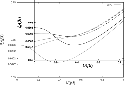
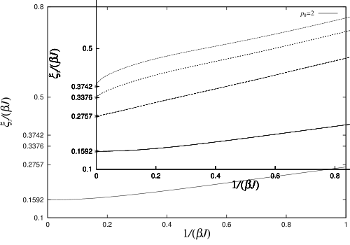
Figure 5: Ratio of the correlation length and the inverse temperature. $\langle\sigma^{+}_{j}\sigma^{-}_{i}\rangle$ (upper) and $\langle\sigma^{z}_{j}\sigma^{z}_{i}\rangle$ (lower) for $p_{0}=3,4,5$ and the free fermion case $p_{0}=2$. The known result (6.16)–(6.17) in the low temperature limit is also depicted by the symbol $\ast$.

References

• [1] M. Suzuki, Prog. Theoret. Phys. 56 (1976) 1454
• [2] M. Suzuki, Phys. Rev. B 31 (1985) 2957.
• [3] M. Suzuki and M. Inoue, Prog. Theor. Phys. 78 (1987) 787.
• [4] M. Inoue and M. Suzuki, Prog. Theor. Phys. 79 (1988) 645.
• [5] T. Koma, Prog. Theor. Phys. 78 (1987) 1213.
• [6] J. Suzuki, Y. Akutsu and M. Wadati, J. Phys. Soc. Japan 59 (1990) 2667.
• [7] J. Suzuki, T. Nagao and M. Wadati, Int. J. Mod. Phys. B 6 (1992) 1119-1180.
• [8] C. Destri and H.J. de Vega, Phys. Rev. Lett. 69 (1992) 2313.
• [9] M. Takahashi, Phys. Rev. B 43 (1991) 5788.
• [10] H. Mizuta, T. Nagao and M. Wadati, J. Phys. Soc. Japan 63 (1994) 3951.
• [11] A. Klümper, Ann. Physik 1 (1992) 540.
• [12] A. Klümper, Z. Phys. B 91 (1993) 507.
• [13] G. Jüttner and A. Klümper, Euro. Phys. Lett. 37(1997) 335.
• [14] G. Jüttner, A. Klümper and J. Suzuki, Nucl. Phys. B 487 (1997) 650.
• [15] G. Jüttner, A. Klümper and J. Suzuki, J. Phys. A. 30 (1997) 1881.
• [16] G. Jüttner, A. Klümper and J. Suzuki, “From fusion hierarchy to excited state TBA” (hep-th/9707074), Nucl. Phys. B in press.
• [17] G. Jüttner, A. Klümper and J. Suzuki, “The Hubbard model at finite temperatures: ab into calculations of Tomonaga-Luttinger liquid property” (cond-mat/9711310)
• [18] M. Takahashi and M. Suzuki, Prog. Theor. Phys. 48 (1972) 2187.
• [19] C.N. Yang and C.P. Yang, J. Math. Phys. 10 (1969) 1115.
• [20] H.L. Eßler, V.E. Korepin and K. Schoutens, J. Phys. A 25 (1992) 4115.
• [21] G. Jüttner and B.D. Dörfel, J. Phys. A 26 (1993) 3105.
• [22] F.C. Alcaraz and M.J. Martins, J. Phys. A 21 (1988) L381, ibid. 4397.
• [23] A. Klümper and P. Pearce, J. Stat. Phys.64 (1991) 13; Physica A 183 (1992) 304.
• [24] A. Kuniba, T. Nakanishi and J. Suzuki, Int. J. Mod. Phys. A 9 (1994) 5267.
• [25] V. E. Korepin, N. M. Bogoliubov and A. G. Izergin, Quantum inverse scattering method and correlation functions, Cambridge Univ. Press (1993).
• [26] P. Fendley, “Excited-state energies and supersymmetric indices”, preprint, hep-th.9706161.
• [27] V.V. Bazhanov, S.L. Lukyanov and A.B. Zamolodchikov, Nucl. Phys. B 489 (1997) 487.
• [28] D. Fioravanti, A. Mariottini, E. Quattrini and F. Ravanini, Phys. Lett B390 (1997) 243.
• [29] A. Kuniba, T. Nakanishi and J. Suzuki, Int. J. Mod. Phys. A 9 (1994) 5215.
• [30] A. Kuniba and T. Nakanishi, Mod. Phys. Lett A 7 (1992) 3487.
• [31] A. Kuniba and J. Suzuki, J. Phys A 28 (1995) 711.
• [32] A. N. Kirillov and N. A. Liskova, J. Phys A 30 (1997) 1209.
• [33] V. Chari and A. Pressley, L’Enseignement Math. 36 (1990) 267.
• [34] R. Tateo Phys.Lett.B 355 (1995) 157.
• [35] A.N. Kirillov and N.Y. Reshetikhin, Zap. Nauch. Semin. LOMI 146 (1985) 31, ibid 47.
• [36] V. E. Korepin, Theor. Math. Phys. 41 (1979) 953.
• [37] S. Katsura, Phys. Rev. 127 (1962) 1508.
• [38] E. Barouch and B.M. McCoy, Phys. Rev. A 3 (1971) 786.
• [39] E. Lieb, T. Schultz and D. Mattis, Ann. Phys. 16 (1961) 406.
Refer to caption
Refer to caption
Refer to caption