Scaling universalities of $k$th-nearest neighbor distances on closed manifolds

Abstract

Take $N$ sites distributed randomly and uniformly on a smooth closed surface. We express the expected distance $\langle D_{k}(N)\rangle$ from an arbitrary point on the surface to its $k$th-nearest neighboring site, in terms of the function $A(l)$ giving the area of a disc of radius $l$ about that point. We then find two universalities. First, for a flat surface, where $A(l)=\pi l^{2}$, the $k$-dependence and the $N$-dependence separate in $\langle D_{k}(N)\rangle$. All $k$th-nearest neighbor distances thus have the same scaling law in $N$. Second, for a curved surface, the average $\int\langle D_{k}(N)\rangle\,d\mu$ over the surface is a topological invariant at leading and subleading order in a large $N$ expansion. The $1/N$ scaling series then depends, up through $O(1/N)$, only on the surface’s topology and not on its precise shape. We discuss the case of higher dimensions ($d>2$), and also interpret our results using Regge calculus.

Key words: stochastic geometry, nearest neighbors

Submitted to Advances in Applied Mathematics, February 1998

1 Introduction

Many problems arising in applied mathematics involve the distance between neighboring sites in a space. One frequently wishes to calculate distances to a nearest neighbor, second-nearest neighbor, and more generally, $k$th-nearest neighbor. Examples in computational geometry and optimization abound, ranging from random packing of spheres to minimum spanning trees. Such problems also occur naturally in physics, and have been considered in applications ranging from stellar dynamics [1], to interactions in liquid systems, to cellular objects such as foams and random lattices [2].

Here we consider the case of $N$ sites placed randomly, with a uniform distribution, on a 2-D surface of fixed area. Let the random variable $D_{k}(N)$ represent the distance between a given point $\mathbf{x}$ and its $k$th-nearest site. The expectation value $\langle D_{k}(N)\rangle$ taken over the ensemble of randomly placed sites — and in fact all moments $\langle D^{\alpha}_{k}(N)\rangle$ — then exhibit some surprising properties. First of all, when the surface is flat $\langle D_{k}(N)\rangle$ may be written, up to corrections exponentially small in $N$, as

$$\langle D_{k}(N)\rangle\approx\frac{1}{\sqrt{\pi}}\,\frac{(k-1/2)!}{(k-1)!}\,\frac{N!}{(N+1/2)!}\mbox{.}$$

This means that the $k$-dependence and the $N$-dependence separate; the large $N$ scaling law for $\langle D_{k}(N)\rangle$ is independent of $k$. Geometrically, the meaning of this universality is far from obvious. Furthermore, the property is not restricted to two dimensions, and turns out to be equally valid for flat spaces of any dimension. Second of all, when the surface is curved, while this $k$-independence no longer holds, one finds on the other hand another universality: if $\langle D_{k}(N)\rangle$ is written in terms of a $1/N$ series, and averaged over the entire surface, the leading and subleading coefficients of the expansion give topological invariants. Thus to $O(1/N)$, the large $N$ scaling law depends not on the detailed shape of the surface but only on the surface’s genus.

In this paper we explore these universalities. We start by expressing $\langle D_{k}(N)\rangle$ in terms of the area, $A(l)$, of a disc of radius $l$ on an arbitrary surface. We observe that in the special case where $A(l)$ consists only of a power of $l$, the scaling law for $\langle D_{k}(N)\rangle$ exhibits the universality in $k$, i.e., is independent of $k$. Then, we give a relation between $A(l)$ and the Gaussian curvature of the surface, and find the leading correction terms in the $1/N$ power series for $\langle D_{k}(N)\rangle$ as functions of the curvature. This results in the topological invariance at $O(1/N)$. We discuss higher order terms as well, and the case of higher dimensions. Finally, we show that a Regge calculus approach provides a simple means of obtaining this topological invariance for the case of polyhedral (non-smooth) surfaces.

2 Preliminaries

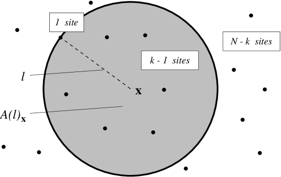
Figure 1: A point $\mathbf{x}$ and its neighborhood within a distance $l$. Area $A(l)_{\mathbf{x}}$ is the probability of finding a site within distance $l$ of $\mathbf{x}$. Here, $k-1$ sites lie within this region, the $k$th-nearest site lies at distance $l$ exactly, and the remaining $N-k$ sites lie outside the region.

Take any point $\mathbf{x}$, and consider $P[D_{k}(N)=l]_{\mathbf{x}}$, the probability density that the point’s $k$th-nearest neighboring site lies at a distance $l$ from it. This is equal to the probability density of having $k-1$ (out of $N$) sites within distance $l$, one site (out of $N-k+1$) at distance $l$, and the remaining $N-k$ sites beyond distance $l$. Let us choose units so that our surface has total area 1. Since sites are distributed uniformly over the surface, the probability of a site lying within distance $l$ is then simply the area $A(l)_{\mathbf{x}}$ of a disc of radius $l$ about point $\mathbf{x}$ on the surface. This is shown in Figure 1. Dropping the argument $\mathbf{x}$ (in order to simplify the notation), we may then write

$$P[D_{k}(N)=l]={N\choose k-1}\,\left[A(l)\right]^{k-1}\times\,{N-k+1\choose 1}\,\frac{dA(l)}{dl}\,\times\,\left[1-A(l)\right]^{N-k},$$

giving the expectation value (first moment)

$$\langle D_{k}(N)\rangle = \int_{0}^{\infty}P[D_{k}(N)=l]\,l\,dl$$

$$= \frac{N!}{(N-k)!\,(k-1)!}\,\int_{0}^{\infty}l\,\left[A(l)\right]^{k-1}\left[1-A(l)\right]^{N-k}\,\frac{dA(l)}{dl}\,dl.$$

Using the variable transformation $w=A(l)$, this may be written in terms of the inverse function $A^{-1}(w)$ as

$$\langle D_{k}(N)\rangle=\frac{N!}{(N-k)!\,(k-1)!}\,\int_{0}^{1}A^{-1}(w)\,w^{k-1}(1-w)^{N-k}\,dw.$$

If $A^{-1}(w)$ admits the power series expansion in $w$:

$$A^{-1}(w)=w^{\gamma}\,\sum_{j=0}^{\infty}c_{j}w^{j},\qquad\mbox{for some }\gamma\in[0,1),$$ (1)

then

$$\langle D_{k}(N)\rangle=\frac{N!}{(N-k)!\,(k-1)!}\,\sum_{j=0}^{\infty}c_{j}\int_{0}^{1}w^{k+j+\gamma-1}(1-w)^{N-k}\,dw.$$ (2)

Recognizing the integral as the Beta function ${\rm B}(k+j+\gamma,N-k+1)=(k+j+\gamma-1)!\,(N-k)!/$ $(N+j+\gamma)!$,

$$\langle D_{k}(N)\rangle=\sum_{j=0}^{\infty}c_{j}\,\frac{(k+j+\gamma-1)!}{(k-1)!}\,\frac{N!}{(N+j+\gamma)!}.$$ (3)

Several comments are in order concerning $\langle D_{k}(N)\rangle$. First of all, although we restrict ourselves to discussing the first moment of $D_{k}(N)$, we could in fact consider any moment $\langle D^{\alpha}_{k}(N)\rangle$ by taking $\left[A^{-1}(w)\right]^{\alpha}$ instead of $A^{-1}(w)$ in (1). Doing so would alter $\gamma$ and the $c_{j}$’s, but would not change our results qualitatively. Second of all, there is no loss of generality in taking our total surface area to be unity; scaling this area by a constant (or even, as might be more intuitive in statistical physics, by $N$) would provide only a trivial scaling factor in our results. Third of all, we could imagine that the point $\mathbf{x}$ we consider is itself an $(N+1)$th site. This is simply a question of nomenclature: the problem of finding the expected distance from an arbitrary point to its kth-nearest site, for a system of $N$ sites, is equivalent to the problem of finding the expected distance between kth-nearest neighboring sites, for a system of $N+1$ sites.

We now turn to the properties of $A^{-1}(w)$, and their consequences on $\langle D_{k}(N)\rangle$.

3 Flat Surfaces

On a flat surface, if we could neglect edge effects, the area included within distance $l$ would simply be $A(l)=\pi l^{2}$. In that case, we would have $A^{-1}(w)=\sqrt{w/\pi}$, and so from (1) and (3),

$$\langle D_{k}(N)\rangle=\frac{1}{\sqrt{\pi}}\,\frac{(k-1/2)!}{(k-1)!}\,\frac{N!}{(N+1/2)!}.$$ (4)

There would thus be a complete separation of the $k$-dependence and the $N$-dependence.

As we are working with a surface of fixed (unit) area, however, we cannot avoid considering edge or finite size effects. Let us restrict ourselves to the case where the surface is everywhere locally Euclidean within some minimum neighborhood of radius $l_{0}>0$. (The simplest example of this is a unit square with periodic boundary conditions, for which $l_{0}=1/2$. Clearly, many other constructions are possible.) Any required modification to the $A^{-1}(w)$ expression in (1) then concerns only $w$ greater than $w_{0}\equiv A(l_{0})$. Correspondingly, (2) remains valid, up to remainder terms from the region of integration $w_{0}\leq w\leq 1$. Since the $(1-w)^{N-k-1}$ term in the integral is bounded above by $(1-w_{0})^{N-k-1}$ within this region, these remainder terms are exponentially small in $N$. Equation (4) is thus still correct to all orders in a $1/N$ series expansion, and may be written as

$$\langle D_{k}(N)\rangle=\frac{1}{\sqrt{\pi}}\,\frac{(k-1/2)!}{(k-1)!}\,\frac{1}{\sqrt{N}}\left[1-\frac{3}{8N}+O\left(\frac{1}{N^{2}}\right)\right],$$

where all orders in the series are independent of $k$. We therefore see that the large $N$ scaling law for $k$th-nearest neighbor distances on a 2-D flat surface without a boundary exhibits the universality in $k$ to all orders in $1/N$.

The same holds true for flat manifolds in any dimension $d$. We assume there is some $l_{0}$ such that the volume included within distance $l<l_{0}$ is simply the volume of a $d$-dimensional ball:

$$A(l) = \frac{\pi^{d/2}\,l^{d}}{(d/2)!},\qquad\mbox{or}$$

$$A^{-1}(w) = \frac{1}{\sqrt{\pi}}\left[w\left(\frac{d}{2}\right)!\right]^{1/d}.$$

As before, this condition allow us to write $\langle D_{k}(N)\rangle$ up to remainder terms that are exponentially small in $N$, so from (3),

$$\langle D_{k}(N)\rangle \approx \frac{\left[(d/2)!\right]^{1/d}}{\sqrt{\pi}}\,\frac{(k-1+1/d)!}{(k-1)!}\,\frac{N!}{(N+1/d)!}$$

$$= \frac{\left[(d/2)!\right]^{1/d}}{\sqrt{\pi}}\,\frac{(k-1+1/d)!}{(k-1)!}\,N^{-1/d}\left[1-\frac{1/d+1/d^{2}}{2N}+O\left(\frac{1}{N^{2}}\right)\right].$$

Thus for flat spaces without a boundary, of any dimension $d$, the universality in $k$ holds to all orders in $1/N$: the $k$-dependence and the $N$-dependence separate.

It may be interesting to consider a slight variation on the problem, giving this universality exactly and not only to all orders. Take the case of a spherical surface embedded in 3-D Euclidean space, with the usual measure of area over the sphere, but with a peculiar sort of “distance”: rather than the conventional choice of the arc length (geodesic) metric, use the chord length. (See Figure 2a.) For a chord of length $l$ originating at a pole of the sphere, the area of the spherical cap spanned by it is simply $A(l)=\pi l^{2}$. The $k$th-nearest neighbor distance properties using chord length “distance” on this curved surface then appear analogous to those on a flat surface. There is, however, one important distinction. The relevant threshold $w_{0}$ for edge effects is in this case $w_{0}=\pi(2R)^{2}$, where $R$ is the radius of the sphere. Since $\pi(2R)^{2}$ is exactly equal to the total surface area of the sphere, it is set to 1. Equation (2) thus requires no corrections at all, and so the universality in (4) is exact.

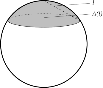
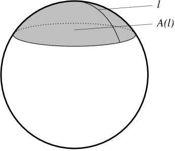
(a) $l$ represents chord length distance	(b) $l$ represents arc length distance

Figure 2: A spherical surface, where $A(l)$ denotes the area of a spherical cap spanned by $l$. In (a), $l$ represents the chord length distance; in (b), $l$ represents the arc length distance.

4 Curved Surfaces

Now consider the case of a surface with intrinsic curvature, with the distance defined in terms of a metric, i.e., along geodesics of the surface. Let us begin with a spherical surface, this time letting $l$ represent arc length; the area of the spherical cap spanned by an arc originating at a pole of the sphere (see Figure 2b) is given by

$$A(l)_{\rm sphere} = 2\pi R^{2}\left[1-\cos\frac{l}{R}\right]$$

$$= 4\pi R^{2}\sin^{2}\frac{l}{2R}.$$

If the total surface area, $4\pi R^{2}$, is normalized to 1,

$$A(l)_{\rm sphere} = \sin^{2}\sqrt{\pi}l,\qquad\mbox{so}$$

$$A^{-1}(w)_{\rm sphere} = \frac{\sin^{-1}\sqrt{w}}{\sqrt{\pi}}$$ (5)

$$\simeq \sqrt{\frac{w}{\pi}}\,\sum_{j=0}^{\infty}\,\frac{w^{j}}{2j+1}\,\frac{(2j)!}{2^{2j}(j!)^{2}}.$$

As in the case of the chord length “distance”, this $A^{-1}(w)$ expression is exact everywhere for $0\leq w\leq 1$. Equations (1) and (3) then require no corrections, and we find

$$\langle D_{k}(N)\rangle_{\rm sphere} = \frac{1}{\sqrt{\pi}}\,\sum_{j=0}^{\infty}\,\frac{1}{2j+1}\,\frac{(2j)!}{2^{2j}(j!)^{2}}\,\frac{(k+j-1/2)!}{(k-1)!}\,\frac{\sqrt{N}\,N!}{(N+j+1/2)!}$$ (6)

$$= \frac{1}{\sqrt{\pi}}\,\frac{(k-1/2)!}{(k-1)!}\,\frac{1}{\sqrt{N}}\left[1+\frac{4k-7}{24N}+O\left(\frac{1}{N^{2}}\right)\right].$$

Clearly, the $k$ universality does not apply here: the $O(1/N)$ coefficient explicitly contains $k$.

Another sort of universality, however, is found when we turn to the more general case of an arbitrary closed surface, i.e., an abstract 2-D manifold with no boundary. Given a smooth surface, we may introduce a system of curvilinear coordinates $u$ and $v$ and write (at least piecewise on the surface) the differential length element $ds$ in the conformal, orthogonal form [3]:

$$ds^{2}=f(u,v)\,[du^{2}+dv^{2}].$$ (7)

The Gaussian curvature $K(u,v)$ of the surface is then expressed in terms of the function $f(u,v)$ by

$$K=\frac{1}{2f^{3}}\left[\left(\frac{\partial f}{\partial u}\right)^{2}+\left(\frac{\partial f}{\partial v}\right)^{2}-f\frac{\partial^{2}f}{\partial u^{2}}-f\frac{\partial^{2}f}{\partial v^{2}}\right].$$ (8)

What is $A(l)$ on this surface? To find out, we first determine the manifold’s geodesic lines. For $ds$ given by (7), we may use the geodesic equation [3]:

$$\frac{d^{2}u}{ds^{2}}+\frac{1}{2f}\,\frac{\partial f}{\partial u}\left[\left(\frac{du}{ds}\right)^{2}-\left(\frac{dv}{ds}\right)^{2}\right]+\frac{1}{f}\,\frac{\partial f}{\partial v}\,\frac{du}{ds}\,\frac{dv}{ds}=0.$$ (9)

Let us expand $u$ and $v$ as functions of distance $s$ from an initial point, along a fixed geodesic:

$$u(s) = u_{0}+su_{0}^{\prime}+\frac{s^{2}}{2}u_{0}^{\prime\prime}+\cdots\quad\mbox{and}$$

$$v(s) = v_{0}+sv_{0}^{\prime}+\frac{s^{2}}{2}v_{0}^{\prime\prime}+\cdots,$$ (10)

where $u_{0}\equiv u(0)$, $u_{0}^{\prime}\equiv u^{\prime}(0)$, etc., and likewise for $v$. Then, expanding $f(u,v)$ in terms of $u$ and $v$ and substituting (10),

$$f(u,v) = f(u_{0},v_{0})+s\left[u_{0}^{\prime}f_{u}(u_{0},v_{0})+v_{0}^{\prime}f_{u}(u_{0},v_{0})\right]+s^{2}\left[\frac{u_{0}^{\prime\prime}}{2}f_{u}(u_{0},v_{0})+\frac{v_{0}^{\prime\prime}}{2}f_{v}(u_{0},v_{0})\right.$$

$$\qquad\left.+\frac{(u_{0}^{\prime})^{2}}{2}f_{uu}(u_{0},v_{0})+u_{0}^{\prime}v_{0}^{\prime}f_{uv}(u_{0},v_{0})+\frac{(v_{0}^{\prime})^{2}}{2}f_{vv}(u_{0},v_{0})\right]+O(s^{3}),$$

where subscripts on $f$ denote partial derivatives.

Using (7) and (9), we can solve for all but three of the coefficients in (10). Let us choose $u_{0}$, $v_{0}$ and $u_{0}^{\prime}$ to be these three. Now, consider the area $A(l)$ about the point $(u_{0},v_{0})$. For $ds$ given in (7), the differential surface element will be $d\mu=f\,du\,dv$, so:

$$A(l) = \int f\,du\,dv$$ (11)

$$= \int f\,J\left(\frac{u,v}{s,u_{0}^{\prime}}\right)ds\,du_{0}^{\prime}$$

$$= \int f\,\left|\frac{\partial u}{\partial s}\frac{\partial v}{\partial u_{0}^{\prime}}-\frac{\partial u}{\partial u_{0}^{\prime}}\frac{\partial v}{\partial s}\right|\,ds\,du_{0}^{\prime}.$$

The limits of integration over $s$ are $0$ and $l$; the limits of integration over $u_{0}^{\prime}$, which may be found from (7), are $-\sqrt{1/f(u_{0},v_{0})}$ and $\sqrt{1/f(u_{0},v_{0})}$. In evaluating the Jacobian some care must be taken, as a sign ambiguity allows two solutions for the coefficients in (10). $A(l)$ will be the sum of (11) evaluated at each of the two solutions, ultimately causing all odd powers of $l$ to vanish.

The result, after lengthy algebraic manipulations, may be written as

$$A(l)=\pi l^{2}\left[1-\frac{l^{2}}{24}\,\frac{1}{f^{3}}\,(f_{u}^{2}+f_{v}^{2}-ff_{uu}-ff_{vv})+O(l^{4})\right],$$ (12)

where in order to avoid cluttering the notation, we have omitted the $(u_{0},v_{0})$ arguments at which all functions are to be evaluated. For the leading correction term in $A(l)$ given in (12), we recognize the expression (8) for the Gaussian curvature $K$. In retrospect, this is not surprising: by symmetry, the correction series to $\pi l^{2}$ can contain only even powers of $l$, and if we consider $A(l)$ as a geometric expansion about a flat space approximation, $K$ will be the only scalar curvature quantity with dimensions of $l^{-2}$ [4].

With some perseverance, one may carry the expansion in (12) to higher orders, obtaining

$$A(l) = \pi l^{2}\left[1-\frac{l^{2}}{12}\,K+\frac{l^{4}}{720}\bigl{(}2K^{2}-3\nabla^{2}K\bigr{)}\right.$$ (13)

$$\qquad\left.-\frac{l^{6}}{161280}\bigl{(}8K^{3}-3[10(\nabla K)^{2}+14K\nabla^{2}K-5\nabla^{4}K]\bigr{)}+O(l^{8})\right],$$

where $\nabla$ is the gradient operator. We thus obtain a series expansion giving the area of a disc on a smooth 2-D surface, in a form that depends only on intrinsic quantities, i.e., not on the choice of coordinate system.

We may invert (13) to obtain the power series

$$A^{-1}(w) = \sqrt{\frac{w}{\pi}}\,\Biggl{[}1+\frac{K}{24\pi}\,w+\frac{9K^{2}+4\nabla^{2}K}{1920\pi^{2}}\,w^{2}+\frac{15K^{3}+14K\nabla^{2}K-2(\nabla K)^{2}+\nabla^{4}K}{21504\pi^{3}}\,w^{3}\Biggr{.}$$ (14)

$$\qquad\Biggl{.}+O(w^{4})\Biggr{]}.$$

As an example, take the special case of a spherical surface, where the Gaussian curvature is a constant $K=1/R^{2}$, or $K=4\pi$ for a unit surface. All derivatives of $K$ then vanish, leaving

$$A^{-1}(w)_{\rm sphere}=\sqrt{\frac{w}{\pi}}\left[1+\frac{w}{6}+\frac{3w^{2}}{40}+\frac{5w^{3}}{112}+O(w^{4})\right],$$

from which we recover the first few terms of our earlier result (5).

Given an expression for $A^{-1}(w)$ on a general 2-D surface, we may now find $\langle D_{k}(N)\rangle$ using (1) and (3). It is helpful at this point to define the reduced variable $\langle\tilde{D}_{k}(N)\rangle$ by dividing out the leading asymptotic (large $N$) behavior from $\langle D_{k}(N)\rangle$. Recalling the notation of (1), $A^{-1}(w)=w^{\gamma}\,\sum_{j}c_{j}w^{j}$ for some $\gamma\in[0,1)$, define:

$$\langle\tilde{D}_{k}(N)\rangle = \langle D_{k}(N)\rangle\,\frac{1}{c_{0}}\,\frac{(k-1)!}{(k+\gamma-1)!}\,N^{\gamma}$$ (15)

$$= N^{\gamma}\,\sum_{j=0}^{\infty}\,\frac{c_{j}}{c_{0}}\,\frac{(k+j+\gamma-1)!}{(k+\gamma-1)!}\,\frac{N!}{(N+j+\gamma)!},$$

so that $\lim_{N\to\infty}\langle\tilde{D}_{k}(N)\rangle=1$ (this is a consequence of Stirling’s law). $\langle\tilde{D}_{k}(N)\rangle$ then corresponds to the $1/N$ power series that we have frequently seen appearing in $\langle D_{k}(N)\rangle$, giving the corrections to its leading (large $N$) behavior. It is in this power series that the interesting universality properties emerge. Consider the average $\int\langle\tilde{D}_{k}(N)\rangle\,d\mu$ over the entire surface, obtained — via (1) and (15) — from precisely the average of the series coefficients in (14). Examine, in particular, the $O(w)$ term of (14). By the Gauss-Bonnet theorem [3], $\int K\,d\mu=2\pi\chi$ on any closed surface, where $\chi$ is the Euler characteristic of the surface, a topological invariant. Up to leading corrections, then,

$$\int A^{-1}(w)\,d\mu = \sqrt{\frac{w}{\pi}}\left[1+\frac{\chi}{12}w+O(w^{2})\right],\qquad\mbox{giving}$$

$$\int\langle\tilde{D}_{k}(N)\rangle\,d\mu = \frac{\sqrt{N}\,N!}{(N+1/2)!}\,\left[1+\frac{\chi}{12}\,\frac{k+1/2}{N+3/2}+O\left(\frac{1}{N^{2}}\right)\right]$$ (16)

$$= 1+\frac{\chi(2k+1)-9}{24N}+O\left(\frac{1}{N^{2}}\right).$$

We thus discover a different sort of universality from the one we had in the case of flat space. To $O(1/N)$, the scaling law for $k$th-nearest neighbor distances depends only on the surface’s topology, and not on its detailed properties.

The Euler characteristic $\chi$ for a surface is related to its genus $g$ by $\chi=2(1-g)$. Taking the torus as one example, $g=1$, so $\chi=0$ and the $k$-dependence in (16) once again disappears, at least at $O(1/N)$. This is to be expected: a flat space with periodic boundary conditions has, after all, the topology of a torus. And conversely, because of the topological invariance, all tori behave like flat space to $O(1/N)$. Taking the spherical surface as another example, $g=0$, so $\chi=2$ and we recover from (16) the power series in (6).

The properties of $\int\langle\tilde{D}_{k}(N)\rangle\,d\mu$ are far less clear at higher orders in $1/N$. Using the divergence theorem and integration by parts, we may obtain from (14)

$$\int A^{-1}(w)\,d\mu=\int\sqrt{\frac{w}{\pi}}\left[1+\frac{K}{24\pi}\,w+\frac{3K^{2}}{640\pi^{2}}\,w^{2}+\frac{15K^{3}+16K\nabla^{2}K}{21504\pi^{3}}\,w^{3}+O(w^{4})\right]\,d\mu.$$ (17)

If we looked only at terms up through $O(w^{2})$, we might believe that this series is simply, by analogy with (5), the expansion of $\int(2/\sqrt{K})\sin^{-1}\sqrt{Kw/4\pi}\,d\mu$. Unfortunately, starting at $O(w^{3})$ we see this is not true, since the contributions of curvature and its gradients do not all vanish in the average over the surface! Furthermore, even for terms in (17) of the form $\int K^{n}\,d\mu$, at $n>1$ there is no straightforward equivalent to the Gauss-Bonnet theorem; the theorem is a direct consequence of the integrand’s linearity. Thus for a general 2-D surface, a simplified form does not appear to exist for the terms in $\int\langle\tilde{D}_{k}(N)\rangle\,d\mu$ beyond $O(1/N)$. More particularly, the only case in which $\int\langle\tilde{D}_{k}(N)\rangle\,d\mu$ would be independent of $k$ beyond $O(1/N)$ is if the curvature is identically equal to $0$, i.e., a flat surface.

Let us briefly consider the case of curved higher-dimensional manifolds. The calculation is now far more complicated, as it is no longer possible to write the metric tensor in a conformal form as we did in (7). In addition, whereas in 2-D the only intrinsic scalar quantity describing curvature is the Gaussian curvature $K$, for $d>2$ there are $d(d-1)(d-2)(d+3)/12$ different such quantities [4]. However, all of them except $K$ itself have dimensions of higher order than $l^{-2}$. It thus seems reasonable to conjecture that, as we argued in 2-D, the $O(l^{2})$ correction term in $A(l)$ can only involve $K$. (Indeed, we have verified that this is true in 3-D.) In that case, we may rely on the example of the spherical surface — easily generalized to $d$ dimensions — to provide us with the initial terms for a general manifold:

$$A(l) = \frac{\pi^{d/2}}{(d/2)!}\,l^{d}\,\left[1-\frac{d(d-1)}{d+2}\,\frac{K}{6}\,l^{2}+O(l^{4})\right],\qquad\mbox{or}$$

$$A^{-1}(w) = \left[\frac{(d/2)!}{\pi^{d/2}}\right]^{1/d}w^{1/d}\,\left[1+\frac{d-1}{d+2}\,\frac{K}{6}\,\left(\frac{(d/2)!}{\pi^{d/2}}\right)^{2/d}\,w^{2/d}+O(w^{4/d})\right].$$ (18)

Note that $A^{-1}(w)$ now contains a series in $w^{2/d}$ rather than in $w$. Appropriately modifying (1), it may then be shown that $\langle\tilde{D}_{k}(N)\rangle$ is in general given by a series in $1/N^{1/d}$ for odd $d$, and $1/N^{2/d}$ for even $d$.

Consider, finally, the average $\int A^{-1}(w)\,d\mu$ over the manifold. The higher-dimensional generalization of the Gauss-Bonnet theorem [5] involves an integrand of $O(1/l^{d})$, or $O(1/w)$. The leading correction term from (18), $\int K\,d\mu$, therefore cannot be simplified further for $d>2$; the only term that could possibly give rise to a topological invariant is the coefficient at $O(l^{d})$, or $O(w)$. If $d$ is odd, it is rather certain that no topological invariant will exist in the series. If $d$ is even, the $O(w)$ term will first contribute to the $\int\langle\tilde{D}_{k}(N)\rangle\,d\mu$ series at $O(1/N)$ — as in 2-D, although at higher dimensions this will no longer be the leading correction term. While one cannot rule out the possibility of obtaining a topological invariant at $O(1/N)$, the $O(w)$ term in $A^{-1}(w)$ is in general a complicated one involving many different curvature scalars, and so this is far from obvious. We leave it as an open question.

5 Regge Calculus

We have remarked that from a physical point of view it is natural, in the 2-D case, for the leading corrections in $A(l)$ to contain only the Gaussian curvature, as this represents the leading deviation from planarity. Consequently, only the mean curvature — or, using the Gauss-Bonnet theorem, the Euler characteristic $\chi$ — matters in the $O(1/N)$ term of $\int\langle\tilde{D}_{k}(N)\rangle\,d\mu$. We have seen using differential methods (geodesics) that this physical picture is indeed correct. These methods apply to a smooth closed surface. For polyhedral surfaces, which are not smooth, we may in fact obtain a similar result more easily, using the non-differential method of Regge calculus. Consider a polyhedron with a number of vertices, edges, and faces. Following the work of Regge [6] and others since then [7], we observe that the curvature is concentrated at the vertices and is measured by a deficit angle: if $\theta_{i}$ is the sum of the angles incident on vertex $i$, the deficit angle at that vertex is $\Delta_{i}=2\pi-\theta_{i}$. It may then be shown that the Gauss-Bonnet theorem, on polyhedra, reduces to Euler’s relation $2\pi\chi=\sum_{i}\Delta_{i}$.

Let $P$ be a polyhedron with a fixed number of vertices, and consider the problem of finding the large $N$ scaling series $\int\langle\tilde{D}_{k}(N)\rangle\,d\mu$ on $P$. As $N\to\infty$, corrections to the flat space value about a given point $\mathbf{x}$ arise only when $\mathbf{x}$ is near one of the vertices, because only in that case can curvature (i.e., the deficit angle) enter into the local calculation of $A(l)$ about $\mathbf{x}$. It is then sufficient to understand the corrections associated with one vertex at a time. Consider the neighborhood of a vertex $i$. $A(l)$ receives a correction from the flat space value, and by a simple geometric construction, one can see that this correction is exactly proportional to the deficit angle $\Delta_{i}$. Correspondingly, the leading correction term both in $A^{-1}(w)$ and in the scaling series will be proportional to $\Delta_{i}$ for small deficit angles. Now sum over all the vertices $i=1,\dots,N$, assuming that all the deficit angles are small. We then find that the $O(1/N)$ term in $\int\langle\tilde{D}_{k}(N)\rangle\,d\mu$ is proportional to $\chi$, and we recover the topological invariant derived in the case of a smooth manifold.

A word of caution is necessary, however. It is tempting at this point to take the limit where $P$ becomes a smooth manifold, expecting to recover (4). Unfortunately this will not work; a direct computation shows that the limit does not commute with the limit $N\to\infty$ taken above, and the coefficient thus obtained at $O(1/N)$ will not be the correct one.

6 Conclusions

Given $N$ sites distributed randomly and uniformly on a surface with no boundaries, we have considered the properties of mean distances to neighboring sites. When the surface is flat, we have seen that in the expression for the mean $k$th-nearest site distance, the $k$-dependence and $N$-dependence separate. The scaling law in $N$ for mean $k$th-nearest neighbor distances is thus independent of $k$. This universality applies equally well to higher moments of the distances, and to Euclidean manifolds in dimensions greater than 2. For surfaces with curvature, while this general property is no longer valid, we have found that when the $k$th-nearest neighbor distance is written as a large $N$ expansion, averaged over the surface, the leading correction term in the series is a topological invariant. The scaling series thus depends, to $O(1/N)$, on the genus of the manifold but not on its other properties.

Although we have considered these universalities only for the moments of point-to-point distances, similar properties hold for higher order simplices such as areas of triangles associated with nearby points. The problem is thus a natural one to consider further in the context of random triangulations, foams or other physical problems [2] tightly connected to geometry.

References

- [1] S. Chandrasekhar, Stochastic problems in physics and astronomy, Rev. Mod. Phys. 15 (1943), 1–89.
- [2] C. Itzykson and J. Drouffe, “Statistical Field Theory,” Cambridge University Press, Cambridge, 1989.
- [3] See, e.g.: E. Kreyszig, “Introduction to Differential Geometry and Riemannian Geometry,” University of Toronto Press, Toronto, 1968; L. P. Eisenhart, “A Treatise on the Differential Geometry of Curves and Surfaces,” Ginn and Company, Boston, 1909.
- [4] S. Weinberg, “Gravitation and Cosmology: Principles and Applications of the General Theory of Relativity,” Wiley, New York, 1972, p. 145.
- [5] L. A. Santalo, “Integral Geometry and Geometric Probability,” Addison-Wesley, Reading, MA, 1976, pp. 302–304; M. Nakahara, “Geometry, Topology and Physics,” A. Holger, Bristol, 1990.
- [6] T. Regge, General relativity without coordinates, Nuovo Cimento 19 (1961), 558–571.
- [7] J. Cheeger, W. Muller and R. Schrader, On the curvature of piecewise flat spaces, Comm. Math. Phys. 92 (1984), 405–454.