The Shape of a Typical Boxed Plane Partition

Abstract.

Using a calculus of variations approach, we determine the shape of a typical plane partition in a large box (i.e., a plane partition chosen at random according to the uniform distribution on all plane partitions whose solid Young diagrams fit inside the box). Equivalently, we describe the distribution of the three different orientations of lozenges in a random lozenge tiling of a large hexagon. We prove a generalization of the classical formula of MacMahon for the number of plane partitions in a box; for each of the possible ways in which the tilings of a region can behave when restricted to certain lines, our formula tells the number of tilings that behave in that way. When we take a suitable limit, this formula gives us a functional which we must maximize to determine the asymptotic behavior of a plane partition in a box. Once the variational problem has been set up, we analyze it using a modification of the methods employed by Logan and Shepp and by Vershik and Kerov in their studies of random Young tableaux.

1. Introduction

In this paper we will show that almost all plane partitions that are constrained to lie within an $a\times b\times c$ box have a certain approximate shape, if $a$, $b$, and $c$ are large; moreover, this limiting shape depends only on the mutual ratios of $a$, $b$, and $c$. Our proof will make use of the equivalence between such plane partitions and tilings of hexagons by rhombuses.

Recall that plane partitions are a two-dimensional generalization of ordinary partitions. A plane partition $\pi$ is a collection of non-negative integers $\pi_{x,y}$ indexed by ordered pairs of non-negative integers $x$ and $y$, such that only finitely many of the integers $\pi_{x,y}$ are non-zero, and for all $x$ and $y$ we have $\pi_{x+1,y}\leq\pi_{x,y}$ and $\pi_{x,y+1}\leq\pi_{x,y}$. A more symmetrical way of looking at a plane partition is to examine the union of the unit cubes $[i,i+1]\times[j,j+1]\times[k,k+1]$ with $i$, $j$, and $k$ non-negative integers satisfying $0\leq k<\pi_{i,j}$. This region is called the solid Young diagram associated with the plane partition, and its volume is the sum of the $\pi_{x,y}$’s.

We say that a plane partition $\pi$ fits within an $a\times b\times c$ box if its solid Young diagram fits inside the rectangular box $[0,a]\times[0,b]\times[0,c]$, or equivalently, if $\pi_{x,y}\leq c$ for all $x$ and $y$, and $\pi_{x,y}=0$ whenever $x\geq a$ or $y\geq b$; we call such a plane partition a boxed plane partition. Plane partitions in an $a\times b\times c$ box are in one-to-one correspondence with tilings of an equi-angular hexagon of side lengths $a,b,c,a,b,c$ by rhombuses whose sides have length $1$ and whose angles measure $\pi/3$ and $2\pi/3$. It is not hard to write down a bijection between the plane partitions and the tilings, but the correspondence is best understood informally, as follows. The faces of the unit cubes that constitute the solid Young diagram are unit squares. Imagine now that we augment the solid Young diagram by adjoining the three “lower walls” of the $a\times b\times c$ box that contains it (namely $\{0\}\times[0,b]\times[0,c]$, $[0,a]\times\{0\}\times[0,c]$, and $[0,a]\times[0,b]\times\{0\}$); imagine as well that each of these walls is divided into unit squares. If we look at this augmented Young diagram from a point on the line $x=y=z$, certain of the unit squares are visible (that is, unobstructed by cubes). These unit squares form a surface whose boundary is the non-planar hexagon whose vertices are the points $(a,0,c)$, $(0,0,c)$, $(0,b,c)$, $(0,b,0)$, $(a,b,0)$, $(a,0,0)$, and $(a,0,c)$, respectively. Moreover, these same unit squares, projected onto the plane $x+y+z=0$ and scaled, become rhombuses which tile the aforementioned planar hexagon. For example, the plane partition $\pi$ in a $2\times 2\times 2$ box defined by $\pi_{0,0}=\pi_{0,1}=\pi_{1,0}=1$ and $\pi_{1,1}=0$ corresponds to the tiling in Figure 1, where the points $(2,0,0)$, $(0,2,0)$, and $(0,0,2)$ are at the lower left, extreme right, and upper left corners of the hexagon. (The shading is meant as an aid for three-dimensional visualization, and is not necessary mathematically. The unshaded rhombuses represent part of the walls.)

Figure 1. The tiling corresponding to a plane partition.

We will use the term $a,b,c$ hexagon to refer to an equi-angular hexagon of side lengths $a,b,c,a,b,c$ (in clockwise order, with the horizontal sides having length $b$), and the term lozenge to refer to a unit rhombus with angles of $\pi/3$ and $2\pi/3$. We will focus, without loss of generality, on those lozenges whose major axes are vertical, which we call vertical lozenges. Although our method in this article is to reduce facts about plane partitions to facts about tilings, one can also go in the reverse direction. For example, one can see from the three-dimensional picture that in every lozenge tiling of an $a,b,c$ hexagon, the number of vertical lozenges is exactly $ac$ (with similar formulas for the other two orientations of lozenge); see [DT] for further discussion.

A classical formula of MacMahon [M] asserts that there are exactly

$$\prod_{i=0}^{a-1}\prod_{j=0}^{b-1}\prod_{k=0}^{c-1}\frac{i+j+k+2}{i+j+k+1}$$

plane partitions that fit in an $a\times b\times c$ box, or (equivalently) lozenge tilings of an $a,b,c$ hexagon. In Theorem 2.2 of this article, we give a generalization that counts lozenge tilings with prescribed behavior on a given horizontal line.

Using Theorem 2.2, we will determine the shape of a typical plane partition in an $a\times b\times c$ box (Theorem 1.2). Specifically, that theorem implies that if $a,b,c$ are large, then the solid Young diagram of a random plane partition in an $a\times b\times c$ box is almost certain to differ from a particular, “typical” shape by an amount that is negligible compared to $abc$ (the total volume of the box). Equivalently, the visible squares in the augmented Young diagram of the random boxed plane partition form a surface whose maximum deviation from a particular, typical surface is almost certain to be $o(\min(a,b,c))$. Moreover, scaling $a,b,c$ by some factor causes the typical shape of this bounding surface to scale by the same factor.

Before we say what the true state of affairs is, we invite the reader to come up with a guess for what this typical shape should be. One natural way to arrive at a guess is to consider the analogous problem for ordinary (rather than plane) partitions. If one considers all ordinary partitions that fit inside an $a\times b$ rectangle (in the sense that their Young diagrams fit inside $[0,a]\times[0,b]$), then it is not hard to show that the typical boundary of the diagram is the line $x/a+y/b=1$; that is, almost all such partitions have roughly triangular Young diagrams. (One way to prove this is to apply Stirling’s formula to binomial coefficients and employ direct counting; another is to use probabilistic methods, aided by a verification that if we look at the boundary of the Young diagram of the partition as a lattice path, then the directions of different steps in the path are negatively correlated.) It therefore might seem plausible that the typical bounding surface for plane partitions would be a plane (except where it coincided with the sides of the box), as when a box is tilted on its corner and half-filled with fluid. However, Theorem 1.1 shows that that is in fact not the case.

To see what a typical boxed plane partition does look like, see Figure 2. This tiling was generated using the methods of [PW] and is truly random, to the extent that pseudo-random number generators can be trusted. Notice that near the corners of the hexagon, the lozenges are aligned with each other, while in the middle, lozenges of different orientations are mixed together. If the bounding surface of the Young diagram tended to be flat, then the central zone of mixed orientations would be an inscribed hexagon, and the densities of the three orientations of tiles would change discontinuously as one crossed into this central zone. In fact, what one observes is that the central zone is roughly circular, and that the tile densities vary continuously except near the midpoints of the sides of the original hexagon.

Figure 2. A random lozenge tiling of a $32,32,32$ hexagon.

One can in theory use our results to obtain an explicit formula for the typical shape of the bounding surface, in which one specifies the distance from a point $P$ on the surface to its image $P^{\prime}$ under projection onto the $x+y+z=0$ plane, as a function of $P^{\prime}$; however, the integral that turns up is quite messy (albeit evaluable in closed form), with the result that the explicit formula is extremely lengthy and unenlightening. Nevertheless, we can and do give a fairly simple formula for the tilt of the tangent plane at $P$ as a function of the projection $P^{\prime}$, which would allow one to reconstruct the surface itself. In view of the correspondence between plane partitions and tilings, specifying the tilt of the tangent plane is equivalent to specifying the local densities of the three different orientations of lozenges for random tilings of an $a,b,c$ hexagon.

Our result on local densities has as a particular corollary the assertion that, in an asymptotic sense, the zone of mixed orientation (defined as the region in which all three orientations of lozenge occur with positive density) is precisely the interior of the ellipse inscribed in the hexagon. This behavior is analogous to what has been proved concerning domino tilings of regions called Aztec diamonds (see [JPS] and [CEP]); these are roughly square regions, and if one tiles them randomly with dominos ($1\times 2$ rectangles), then the zone of mixed orientation tends in the limit to the inscribed disk. However, the known results for Aztec diamonds are stronger than the corresponding best known results for hexagons (see Conjecture 6.2 in Section 6).

To state our main theorem, we begin by setting up normalized coordinates. Suppose that we are dealing with an $a,b,c$ hexagon, so that the side lengths are $a,b,c,a,b,c$ in clockwise order (with the sides of length $b$ horizontal). We let $a,b,c$ tend to infinity together, in such a way that the three-term ratio $a:b:c$ (i.e., element of the projective plane ${\mathbb{P}}^{2}({\mathbb{R}})$) converges to $\alpha:\beta:\gamma$ for some fixed positive numbers $\alpha$, $\beta$, $\gamma$. Say $a+b+c=\sigma(\alpha+\beta+\gamma)$ for some scaling factor $\sigma$. Then we choose re-scaled coordinates for the $a,b,c$ hexagon so that its sides are $a^{\prime}=a/\sigma$, $b^{\prime}=b/\sigma$, and $c^{\prime}=c/\sigma$ (which by the hypothesis of our main theorem will be required to converge to $\alpha$, $\beta$, and $\gamma$ as $a$, $b$, and $c$ get large). Note that $a^{\prime},b^{\prime},c^{\prime}$ in general are not integers. The origin of our coordinate system lies at the center of the hexagon. One can check that the sides of the hexagon lie on the lines $y=\frac{\sqrt{3}}{2}(2x+b^{\prime}+c^{\prime})$, $y=\frac{\sqrt{3}}{4}(a^{\prime}+c^{\prime})$, $y=\frac{\sqrt{3}}{2}(-2x+a^{\prime}+b^{\prime})$, $y=\frac{\sqrt{3}}{2}(2x-b^{\prime}-c^{\prime})$, $y=\frac{\sqrt{3}}{4}(-a^{\prime}-c^{\prime})$, and $y=\frac{\sqrt{3}}{2}(-2x-a^{\prime}-b^{\prime})$, and that the inscribed ellipse is described by

$$3(a^{\prime}+c^{\prime})^{2}x^{2}-2\sqrt{3}(a^{\prime}+2b^{\prime}+c^{\prime})(a^{\prime}-c^{\prime})xy+((a^{\prime}+2b^{\prime}+c^{\prime})^{2}-4a^{\prime}c^{\prime})y^{2}=3a^{\prime}b^{\prime}c^{\prime}(a^{\prime}+b^{\prime}+c^{\prime}).$$

Define $E_{\alpha,\beta,\gamma}(x,y)$ to be the polynomial

$$3\alpha\beta\gamma(\alpha+\beta+\gamma)-(3(\alpha+\gamma)^{2}x^{2}-2\sqrt{3}(\alpha+2\beta+\gamma)(\alpha-\gamma)xy+((\alpha+2\beta+\gamma)^{2}-4\alpha\gamma)y^{2}),$$

whose zero-set is the ellipse inscribed in the $\alpha,\beta,\gamma$ hexagon. Also define $Q_{\alpha,\beta,\gamma}(x,y)$ to be the polynomial

$$\frac{\sqrt{3}}{2}\left(\frac{4}{3}y^{2}-4x^{2}+\beta^{2}+\alpha\beta+\beta\gamma-\alpha\gamma\right),$$

which will be useful shortly.

There are six points at which the ellipse inscribed in the $\alpha,\beta,\gamma$ hexagon meets the boundary of the hexagon. The four that occur on sides of length $\alpha$ or $\gamma$ will be called singular points, for reasons that will be clear shortly. (Recall that we have already broken the underlying symmetry of the situation by agreeing to focus on vertical lozenges.) The points of the hexagon that lie outside the inscribed ellipse form six connected components. Let $R_{1}$ be the closure of the union of the two components containing the leftmost and rightmost points of the hexagon, minus the four singular points, and let $R_{0}$ be the closure of the union of the other four components, again minus the four singular points.

Finally, define the (normalized) coordinates of a vertical lozenge to be the (normalized) coordinates of its center. Then the following theorem holds:

Theorem 1.1.

Let $U$ be the interior of a smooth simple closed curve contained inside the $\alpha,\beta,\gamma$ hexagon, with $\alpha,\beta,\gamma>0$. In a random tiling of an $a,b,c$ hexagon, as $a,b,c\rightarrow\infty$ with $a:b:c\rightarrow\alpha:\beta:\gamma$, the expected number of vertical lozenges whose normalized coordinates lie in $U$ is $ab+bc+ac$ times

$$\frac{1}{A}\iint_{\!U}{\mathcal{P}}_{\alpha,\beta,\gamma}(x,y)\,dx\,dy\,+\,o(1),$$

where $A=(\alpha\beta+\beta\gamma+\alpha\gamma)\sqrt{3}/2$ is the area of the $\alpha,\beta,\gamma$ hexagon and

$${\mathcal{P}}_{\alpha,\beta,\gamma}(x,y)=\begin{cases}\displaystyle\frac{1}{\pi}\cot^{-1}\!\left(\frac{Q_{\alpha,\beta,\gamma}(x,y)}{\sqrt{E_{\alpha,\beta,\gamma}(x,y)}}\right)&\textup{if $E_{\alpha,\beta,\gamma}(x,y)>0$,}\\ 0&\textup{if $(x,y)\in R_{0}$, and}\\ 1&\textup{if $(x,y)\in R_{1}$}.\\ \end{cases}$$

In fact, our proof will give an even stronger version of Theorem 1.1, in which $U$ is a horizontal line segment rather than an open set (and the double integral is replaced by a single integral). Since we can derive the expected number of vertical lozenges whose normalized coordinates lie in $U$ by integrating over all horizontal cross sections (provided that the error term is uniform for all cross sections, as we will prove in Section 4), this variant of the claim implies the one stated above, though it is not obviously implied by it. We have stated the result in terms of open sets because that formulation seems more natural; the proof just happens to tell us more.

The intuition behind Theorem 1.1 is that ${\mathcal{P}}_{\alpha,\beta,\gamma}(x,y)$ gives the density of vertical lozenges in the normalized vicinity of $(x,y)$; the factor of $ab+bc+ac$ arises simply because there are that many lozenges in a tiling of an $a,b,c$ hexagon. One might be tempted to go farther and think of ${\mathcal{P}}_{\alpha,\beta,\gamma}(x,y)$ as the asymptotic probability that a random tiling of the $a,b,c$ hexagon will have a vertical lozenge at any particular location in the normalized vicinity of $(x,y)$ (see Conjecture 6.1 in Section 6); however, we cannot justify this interpretation rigorously, because it is conceivable that there are small-scale fluctuations in the probabilities that disappear in the double integral. (In Subsection 1.3 of [CEP], it is shown that the analogous probabilities for random domino tilings do exhibit such fluctuations, although the fluctuations disappear if one distinguishes between four classes of dominos, rather than just horizontal and vertical dominos.)

The formula for ${\mathcal{P}}_{\alpha,\beta,\gamma}$ is more natural than it might appear. Examination of random tilings such as the one shown in Figure 2 leads one to conjecture that the region in which all three orientations of lozenges occur with positive density is (asymptotically) the interior of the ellipse inscribed in the hexagon, and the known fact that an analogous claim holds for random domino tilings of Aztec diamonds (see [CEP]) lends further support to this hypothesis. This leads one to predict that ${\mathcal{P}}_{\alpha,\beta,\gamma}$ will be $0$ in $R_{0}$ and $1$ in $R_{1}$, and strictly between $0$ and $1$ in the interior of the ellipse. Comparison with the analogous theorem for domino tilings (Theorem 1 of [CEP]) suggests that within the inscribed ellipse, ${\mathcal{P}}_{\alpha,\beta,\gamma}(x,y)$ should be of the form

$$\frac{1}{\pi}\cot^{-1}\left(\frac{Q(x,y)}{\sqrt{E_{\alpha,\beta,\gamma}(x,y)}}\right)$$

for some quadratic polynomial $Q(x,y)$, and the only problem is actually finding $Q(x,y)$ in terms of $\alpha,\beta,\gamma$. A simple description of the polynomial $Q(x,y)$ that actually works is that its zero-set is the unique hyperbola whose asymptotes are parallel to the non-horizontal sides of the hexagon and which goes through the four points on the boundary of $R_{1}$ where the inscribed ellipse is tangent to the hexagon. This determines $Q(x,y)$ up to a constant factor, and that constant factor is determined (at least in theory—in practice the calculations would be cumbersome) by requiring that the average of ${\mathcal{P}}_{\alpha,\beta,\gamma}(x,y)$ over the entire hexagon must be $\alpha\gamma/(\alpha\beta+\beta\gamma+\alpha\gamma)$.

An alternative way to phrase Theorem 1.1 is in terms of height functions, which were introduced by Thurston in [Th] as a geometrical tool for understanding tilings of regions by lozenges or dominos. A height function is a numerical representation of an individual tiling of a specified region. In the case of lozenge tilings of a hexagon, the vertices of the lozenges occur at points of a certain triangular lattice that is independent of the particular tiling chosen, and the height function simply associates a certain integer to each such vertex so as to describe the shape of the plane partition that corresponds to the tiling. Given any lozenge tiling, one can assign heights $h(u)$ to the points $u$ of the triangular lattice as follows. Give the leftmost vertex of the hexagon height $a+c$. (We choose this height so that the vertex of the bounding box farthest from the viewer, which is usually obscured from view, will have height $0$.) Suppose that $u$ and $v$ are adjacent lattice points, such that the edge connecting them does not bisect a lozenge. If the edge from $u$ to $v$ points directly to the right, set $h(v)=h(u)+1$, and if it points up and to the right, or down and to the right, set $h(v)=h(u)-1$. (If it points left, change $+1$ to $-1$ and vice versa.) If one traces around each lozenge in the tiling and follows this rule, then every vertex is assigned a height. It is not hard to check that the heights are well-defined, so there is a unique height function associated to the tiling. For an example, see Figure 3. Conversely, every way of assigning integer heights to the vertices of the triangular grid that assigns height $a+c$ to the leftmost vertex of the hexagon and that satisfies the edge relation must be the height function associated to some unique tiling. If one views the tiling as a three-dimensional picture of the solid Young diagram of a plane partition, then the height function tells how far above a reference plane (of the form $x+y+z=\mbox{constant}$) each vertex lies. The values of the height function on the boundary of the hexagon are constrained, but all the values in the interior genuinely depend on the tiling. (It should be mentioned that height functions for lozenge tilings are implicit in the work of physicists Blöte and Hilhorst, in the context of the two-dimensional dimer model on a hexagonal lattice; see [BH].)

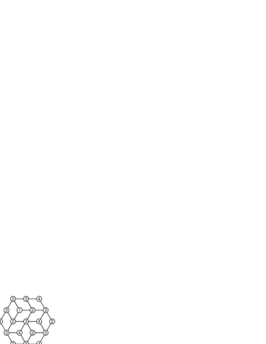
Figure 3. The height function corresponding to a tiling.

When dealing with normalized coordinates, it is convenient to use a normalized height function: if we scale the coordinates by dividing them by $\sigma$ (as described above), then we also divide the height function values by $\sigma$. Also, we define the average height function to be the average of the height functions associated with all possible tilings. (Of course, it is not a height function itself.) We will show that almost every height function closely approximates the average height function, asymptotically:

Theorem 1.2.

Fix $\alpha,\beta,\gamma>0$. As $a,b,c\rightarrow\infty$ with $a:b:c\rightarrow\alpha:\beta:\gamma$, the normalized average height function of the $a,b,c$ hexagon converges uniformly to the function ${\mathcal{H}}_{\alpha,\beta,\gamma}$ with the appropriate (piecewise linear) boundary conditions such that

$$\frac{\partial{\mathcal{H}}_{\alpha,\beta,\gamma}(x,y)}{\partial x}=1-3{\mathcal{P}}_{\alpha,\beta,\gamma}(x,y).$$

For fixed $\varepsilon>0$, the probability that the normalized height function of a random tiling will differ anywhere by more than $\varepsilon$ from ${\mathcal{H}}_{\alpha,\beta,\gamma}$ is exponentially small in $\sigma^{2}$, where $\sigma=(a+b+c)/(\alpha+\beta+\gamma)$.

It is not hard to deduce Theorem 1.2 (with the exception of the claim made in the last sentence) from Theorem 1.1; in particular, the differential equation simply results from considering how the height changes as one crosses lozenges of each orientation. We will give the proof in detail in Section 4.

Unfortunately, although one can recover an explicit formula for ${\mathcal{H}}_{\alpha,\beta,\gamma}(x,y)$ from the boundary values and the knowledge of ${\partial{\mathcal{H}}_{\alpha,\beta,\gamma}(x,y)}/{\partial x}$, we cannot find any simple formula for it. By contrast, Proposition 17 of [CEP] gives a comparatively simple asymptotic formula for the average height function for domino tilings of an Aztec diamond.

Our methods also apply to the case of random domino tilings of Aztec diamonds. Formula (7) of Section 4 of [EKLP] is analogous to our Theorem 2.2, and can be used in the same way. It turns out that the functional arrived at by applying the methods of Section 3 of this paper to that formula is very similar to the one we will find in Section 3. After a simple change of variables, one ends up with essentially the same functional, but maximized over a slightly different class of functions. The methods of Section 4 apply almost without change, and the methods of Section 5 can be adapted to prove Proposition 17 of [CEP]. This proof is shorter than the one given in [CEP]; however, in [CEP], Proposition 17 comes as a corollary of a much stronger result (Theorem 1), which the methods of this paper do not prove.

2. The Product Formula

In this section, we will prove a refinement of MacMahon’s formula, following methods first used by Elkies et al. in [EKLP]. This refinement (Proposition 2.1) is not strictly speaking new, since it is really nothing more than the Weyl dimension formula for finite-dimensional representations of $\mbox{SL}(n)$ (we say a few words more about this connection below). However, we give our own proof of this result for two reasons: first, to make this part of the proof self-contained; and second, to illustrate an expeditious method of proof that has found applications elsewhere (see [JP] for related formulas derived by the same method).

Proposition 2.1 is stated in terms of Gelfand patterns, so we must first explain what Gelfand patterns are and what they have to do with lozenge tilings. It is not hard to see that a lozenge tiling of a hexagon is determined by the locations of its vertical lozenges. A semi-strict Gelfand pattern is a way to keep track of these locations. Specifically, one augments the $a,b,c$ hexagon by adding $a(a+1)/2$ vertical lozenges on the left and $c(c+1)/2$ vertical lozenges on the right, forming an approximate trapezoid of upper base $a+b+c$ and lower base $b$, with some triangular protrusions along its upper border, as in Figure 4. One then associates with each vertical lozenge in the tiling the horizontal distance from its right corner to the left border of the trapezoid, which we call its trapezoidal position. (When we want to use the left boundary of the hexagon instead of the left boundary of the approximate trapezoid as our bench mark, we will speak of the hexagonal position of a vertical lozenge.) For example, consider the tiling shown in Figure 1; we augment it by adding $6$ vertical lozenges to form the tiling shown in Figure 4. The vertical lozenges form rows, and the only restriction on their placement is that given any two adjacent vertical lozenges in the same row, there must be exactly one vertical lozenge between them in the row immediately beneath them. If we index the locations of the vertical lozenges with their trapezoidal positions (the numbers shown in Figure 4), we arrive at the following semi-strict Gelfand pattern:

$$\begin{array}[]{ccccccc}1&&2&&5&&6\\ &&&&&&\\ &1&&2&&5&\\ &&&&&&\\ &&1&&4&&\\ &&&&&&\\ &&&2&&&\\ \end{array}$$

Figure 4. The semi-strict Gelfand pattern corresponding to a tiling.

In general, a semi-strict Gelfand pattern is a triangular array of integers (such as this one), with the property that the entries increase weakly along diagonals running down and to the right, and the entries increase strictly along diagonals running up and to the right. As discussed above, there is a simple bijection between semi-strict Gelfand patterns with top row $1,2,\dots,a,a+b+1,a+b+2,\dots,a+b+c$ and lozenge tilings of an equi-angular hexagon with side lengths $a,b,c,a,b,c$.

Moreover, consider the $k$-th horizontal line from the top in an $a,b,c$ hexagon, where the top edge of the hexagon corresponds to $k=0$, so that the trapezoidal positions of the vertical lozenges on the $k$-th line are precisely the entries in the $(k+1)$-st row of the associated semi-strict Gelfand pattern. If we discard all lozenges that lie above the line (but retain all vertical lozenges that are bisected by it and all lozenges that lie below it), then we get a tiling of a smaller approximate trapezoid, whose upper border as before consists of triangular protrusions alternating with straight edges, except that now the protrusions need not be concentrated at the left and right portions of the border. The trapezoidal positions of the vertical lozenges in this tiling are given by the entries in the semi-strict Gelfand pattern obtained from the original semi-strict Gelfand pattern by deleting the first $k$ rows. In fact, if we limit ourselves to tilings of the $a,b,c$ hexagon in which the locations of the vertical lozenges that are bisected by the $k$-th horizontal line are specified, then each individual tiling of this kind corresponds to a pair of semi-strict Gelfand patterns. We have already described one of these Gelfand patterns, which gives the behavior of the tiling below the cutting line; the other, which describes the tilings above the line, comes from reflecting the hexagon through the horizontal axis (and of course adjoining additional lozenges, as above). If $0\leq k<\min(a,c)$, then one of the Gelfand patterns will include some of the augmenting vertical lozenges described above on both sides (a row of length $a-k$ on one side of the top of the pattern, and a row of length $c-k$ on the other) and the other pattern will contain augmenting vertical lozenges on neither side; if $\min(a,c)\leq k\leq(a+c)/2$, then one of the Gelfand patterns will contain a row of $|a-k|$ augmenting lozenges on one side and the other Gelfand pattern will contain $|c-k|$ on the other side. (The case $k>(a+c)/2$ is symmetric to the case $k<(a+c)/2$, so we do not treat it explicitly.)

In Theorem 2.2, we will use the following formula to determine how many tilings have a specified distribution of vertical lozenges along a horizontal line.

Proposition 2.1.

There are exactly

$$\prod_{1\leq i<j\leq n}\frac{x_{j}-x_{i}}{j-i}$$

semi-strict Gelfand patterns with top row consisting of integers $x_{1},x_{2},\dots,x_{n}$ such that $x_{1}<x_{2}<\dots<x_{n}$.

Proposition 2.1 has an explanation in terms of representation theory. Gelfand and Tsetlin [GT] show that semi-strict Gelfand patterns form bases of representations of $\mbox{SL}(n)$, and one can deduce Proposition 2.1 from this fact using the Weyl dimension formula. (The Gelfand patterns in [GT] are not semi-strict, but there is an easy transformation that makes them so: Replace $m_{p,q}$ in equation (3) of [GT] with $m_{p,q}+(q-p)$ and then reflect the triangle through its vertical axis.) Thus, the novelty of our approach is not that one can count semi-strict Gelfand patterns, but rather that one can count tilings with prescribed behavior on a horizontal line (as in Theorem 2.2). Another proof of Proposition 2.1, and one that bypasses its representation-theoretic significance, is the article of Carlitz and Stanley [CS]. (That article does not deal directly with semi-strict Gelfand patterns, but it is easy to deduce Proposition 2.1 from the theorem proved there.)

Proof.

Let $V(x_{1},\dots,x_{n})$ be the number of semi-strict Gelfand patterns with top row $x_{1},\dots,x_{n}$. Given any such pattern, the second row must be of the form $y_{1},\dots,y_{n-1}$ with $x_{i}\leq y_{i}<x_{i+1}$ for all $i$. Therefore,

(2.1) $$V(x_{1},\dots,x_{n})=\!\!\mathop{{\,\,\,}{\sum}^{{}_{L}}}_{y_{1}=x_{1}}^{x_{2}}\!\!\mathop{{\,\,\,}{\sum}^{{}_{L}}}_{y_{2}=x_{2}}^{x_{3}}\dots\!\!\mathop{{\,\,\,}{\sum}^{{}_{L}}}_{y_{n-1}=x_{n-1}}^{x_{n}}V(y_{1},\dots,y_{n-1}),$$

where the modified summation operator $\!\!\mathop{{\,\,\,}{\sum}^{{}_{L}}}$ is defined by

$$\!\!\mathop{{\,\,\,}{\sum}^{{}_{L}}}_{i=s}^{t}f(i)=\sum_{i=s}^{t-1}f(i).$$

The advantage to writing it this way is that

(2.2) $$\!\!\mathop{{\,\,\,}{\sum}^{{}_{L}}}_{i=r}^{s}f(i)+\!\!\mathop{{\,\,\,}{\sum}^{{}_{L}}}_{i=s}^{t}f(i)=\!\!\mathop{{\,\,\,}{\sum}^{{}_{L}}}_{i=r}^{t}f(i)$$

whenever $r<s<t$. There is a unique way to extend the definition of

$$\!\!\mathop{{\,\,\,}{\sum}^{{}_{L}}}_{i=s}^{t}f(i)$$

to the case $s>t$, if we require that (2.2) be true for all $r,s,t$. Then starting from the base relation $V(x_{1})=1$, we can use (2.1) to define $V(x_{1},\dots,x_{n})$ for arbitrary integers $x_{1},\dots,x_{n}$ (not necessarily satisfying $x_{1}<\dots<x_{n}$).

We will prove the formula for $V(x_{1},\dots,x_{n})$ by induction on $n$. It is clearly true for $n=1$. Suppose that for all $y_{1},\dots,y_{n-1}$,

(2.3) $$V(y_{1},\dots,y_{n-1})=\prod_{1\leq i<j\leq n-1}\frac{y_{j}-y_{i}}{j-i}.$$

Then $V(y_{1},\dots,y_{n-1})$ is a polynomial of total degree $(n-1)(n-2)/2$ in $y_{1},\dots,y_{n-1}$. When we put (2.3) into (2.1), we find that after each of the $n$ summations in (2.1), the result is still a polynomial, and the degree increases by $1$ each time. It is easy to check from (2.3) that the coefficient of $y_{2}^{1}y_{3}^{2}\dots y_{n-1}^{n-2}$ in $V(y_{1},\dots,y_{n-1})$ is

$$\frac{1}{1!2!\dots(n-2)!}.$$

From this and (2.1) it follows that the coefficient of $x_{2}^{1}x_{3}^{2}\dots x_{n}^{n-1}$ in $V(x_{1},\dots,x_{n})$ is

$$\frac{1}{1!2!\dots(n-1)!}.$$

We have therefore shown that $V(x_{1},\dots,x_{n})$ and

(2.4) $$\prod_{1\leq i<j\leq n}\frac{x_{j}-x_{i}}{j-i}$$

are polynomials in $x_{1},\dots,x_{n}$ of the same total degree, and with the same coefficient of $x_{2}^{1}x_{3}^{2}\dots x_{n}^{n-1}$. If we can show that $V(x_{1},\dots,x_{n})$ is divisible by (2.4), then they must be equal. Equivalently, we just need to show that $V(x_{1},\dots,x_{n})$ is skew-symmetric in $x_{1},\dots,x_{n}$.

For convenience, let $(s_{1},t_{1};s_{2},t_{2};\dots;s_{n-1},t_{n-1})$ denote

$$\!\!\mathop{{\,\,\,}{\sum}^{{}_{L}}}_{y_{1}=s_{1}}^{t_{1}}\!\!\mathop{{\,\,\,}{\sum}^{{}_{L}}}_{y_{2}=s_{2}}^{t_{2}}\dots\!\!\mathop{{\,\,\,}{\sum}^{{}_{L}}}_{y_{n-1}=s_{n-1}}^{t_{n-1}}V(y_{1},y_{2},\dots,y_{n-1}).$$

We want to show that $(x_{1},x_{2};x_{2},x_{3};\dots;x_{n-1},x_{n})$ is skew-symmetric in $x_{1},\dots,x_{n}$.

To start off, notice that for all $i$,

(2.5) $$(\dots;s_{i},u_{i};\dots)=(\dots;s_{i},t_{i};\dots)+(\dots;t_{i},u_{i};\dots).$$

Also, since $V(y_{1},\dots,y_{n-1})$ is a skew-symmetric function of $y_{1},\dots,y_{n-1}$ by (2.3), for $i<j$ we must have

$$(\dots;s_{i},t_{i};\dots;s_{j},t_{j};\dots)=-(\dots;s_{j},t_{j};\dots;s_{i},t_{i};\dots).$$

The relation $(\dots;s_{i},t_{i};\dots)=-(\dots;t_{i},s_{i};\dots)$ follows easily from the definition of $(\dots;s_{i},t_{i};\dots)$. From the last two relations, we see that $(\dots;s_{i},t_{i};\dots;s_{j},t_{j};\dots)$ vanishes if $s_{i}=s_{j}$ and $t_{i}=t_{j}$, or if $s_{i}=t_{j}$ and $s_{j}=t_{i}$.

To verify that $(x_{1},x_{2};\dots;x_{n-1},x_{n})$ is skew-symmetric in $x_{1},\dots,x_{n}$, it suffices to check that it changes sign under transpositions of adjacent $x_{i}$’s. We check the effect of exchanging $x_{i+1}$ with $x_{i+2}$ as follows. If we write $x^{\prime}_{k}=x_{i+k}$ (to simplify the subscripts), we have

$$(\dots;x^{\prime}_{0},x^{\prime}_{2};x^{\prime}_{2},x^{\prime}_{1};x^{\prime}_{1},x^{\prime}_{3};\dots) = \phantom{\phantom{}+\phantom{}}(\dots;x^{\prime}_{0},x^{\prime}_{1};x^{\prime}_{2},x^{\prime}_{1};x^{\prime}_{1},x^{\prime}_{2};\dots)$$

$$\phantom{}+(\dots;x^{\prime}_{0},x^{\prime}_{1};x^{\prime}_{2},x^{\prime}_{1};x^{\prime}_{2},x^{\prime}_{3};\dots)$$

$$\phantom{}+(\dots;x^{\prime}_{1},x^{\prime}_{2};x^{\prime}_{2},x^{\prime}_{1};x^{\prime}_{1},x^{\prime}_{2};\dots)$$

$$\phantom{}+(\dots;x^{\prime}_{1},x^{\prime}_{2};x^{\prime}_{2},x^{\prime}_{1};x^{\prime}_{2},x^{\prime}_{3};\dots).$$

by several applications of (2.5). All terms on the right except the second are $0$, so

$$(\dots;x^{\prime}_{0},x^{\prime}_{2};x^{\prime}_{2},x^{\prime}_{1};x^{\prime}_{1},x^{\prime}_{3};\dots) = (\dots;x^{\prime}_{0},x^{\prime}_{1};x^{\prime}_{2},x^{\prime}_{1};x^{\prime}_{2},x^{\prime}_{3};\dots)$$

$$= -(\dots;x^{\prime}_{0},x^{\prime}_{1};x^{\prime}_{1},x^{\prime}_{2};x^{\prime}_{2},x^{\prime}_{3};\dots).$$

Thus, exchanging $x_{i+1}$ with $x_{i+2}$ introduces a minus sign whenever $i\geq 1$ and $i+3\leq n$. The other cases (exchanging $x_{1}$ with $x_{2}$ or $x_{n-1}$ with $x_{n}$) are easily dealt with in a similar way. Therefore, $V(x_{1},\dots,x_{n})$ is skew-symmetric in $x_{1},\dots,x_{n}$, so as discussed above we must have

$$V(x_{1},\dots,x_{n})=\prod_{1\leq i<j\leq n}\frac{x_{j}-x_{i}}{j-i},$$

as desired. ∎

Notice that after some manipulation of the product

$$V(1,2,\dots,a,a+b+1,a+b+2,\dots,a+b+c),$$

Proposition 2.1 implies MacMahon’s formula. However, our main application will be to counting tilings with prescribed behavior on horizontal lines.

Consider the $k$-th horizontal line from the top in an $a,b,c$ hexagon. If $k<\min(a,c)$, then in every tiling there must be $k$ vertical lozenges on the $k$-th line; if $\min(a,c)\leq k\leq(a+c)/2$, then there must be $\min(a,c)$ vertical lozenges on it. (As mentioned earlier, symmetry frees us from needing to treat the case $k>(a+c)/2$, so we will routinely assume $k\leq(a+c)/2$.) In either case, note that the number of vertical lozenges on the $k$-th row is $\min(k,a,c)$.

Define the function

$$V(x_{1},\dots,x_{n})=\prod_{1\leq i<j\leq n}\frac{x_{j}-x_{i}}{j-i},$$

as in the proof of Proposition 2.1. Then we have the following formulas:

Theorem 2.2.

Suppose we require that the vertical lozenges bisected by the $k$-th horizontal line from the top in an $a,b,c$ hexagon occur at hexagonal positions $1\leq a_{1}<a_{2}<\dots<a_{\ell}\leq b+\min(k,a)$ (and nowhere else), with $\ell=\min(k,a,c)$. If $k<\min(a,c)$, there are

$$V(a_{1},a_{2},\dots,a_{\ell})V(1,2,\dots,a-k,a-k+a_{1},\dots,a-k+a_{\ell},a+b+1,\dots,a+b+c-k)$$

such tilings. If $a\leq c$ and $a\leq k\leq(a+c)/2$, there are

$$V(1,2,\dots,k-a,k-a+a_{1},\dots,k-a+a_{\ell})V(a_{1},a_{2},\dots,a_{\ell},a+b+1,\dots,a+b+c-k)$$

such tilings (and a similar formula applies if $c<a$ and $c\leq k\leq(a+c)/2$).

For the proof, simply notice that tilings of the parts of the hexagon above and below the $k$-th line correspond naturally to semi-strict Gelfand patterns with certain top rows, and then apply Proposition 2.1 to count them. In both cases, the two factors correspond to the parts of the tiling that lie above and below the cutting line.

3. Setting up the Functional

We now turn to the proofs of our main theorems. As is usually done in situations such as ours, where one seeks to establish a law of large numbers for some class of combinatorial objects, we approach the problem by trying to find the individually most likely outcome (in this case, the individually most likely behavior of the height function on a fixed horizontal line), and showing that outcomes that differ substantially from it are very unlikely, even considered in aggregate. We will begin in this section by setting up a functional to be maximized; the function that maximizes it will be a simple transformation of the average height function.

Our method is to focus on the locations of the vertical lozenges rather than the height function per se. The two are intimately related, because, as we move across the tiling from left to right, the (unnormalized) height decreases by 2 when we cross a vertical lozenge and increases by 1 when we fail to cross a vertical lozenge. Thus, in determining the likely locations of vertical lozenges, we will in effect be solving for the average height function. Theorem 2.2 tells us that we can count tilings with prescribed behavior on horizontal lines, so we will start off by taking the logarithm of the product formula in Theorem 2.2 and interpreting it as a Riemann sum for a double integral.

In fact, it will be convenient to look first at a more general product, and then apply our analysis of it to the product appearing in Theorem 2.2. Fix positive integers $\ell$ and $n$ satisfying $\ell\leq n$, and non-negative integers $n_{L}$ and $n_{R}$. We will try to determine the distribution of $(a_{1},a_{2},\dots,a_{\ell})$ satisfying $1\leq a_{1}<a_{2}<\dots<a_{\ell}\leq n$ that maximizes

$$V(1,2,\dots,n_{L},n_{L}+a_{1},n_{L}+a_{2},\dots,n_{L}+a_{\ell},n_{L}+n+1,n_{L}+n+2,\dots,n_{L}+n+n_{R}).$$

For convenience, let $b_{i}$ denote the $i$-th element of the sequence $1,2,\dots,n_{L},n_{L}+a_{1},\dots,n_{L}+a_{\ell},n_{L}+n+1,\dots,n_{L}+n+n_{R}$.

Set $\rho_{L}=n_{L}/n$, $\lambda=\ell/n$, and $\rho_{R}=n_{R}/n$. We will work in the limit as $n\rightarrow\infty$, with $\rho_{L}$, $\lambda$, and $\rho_{R}$ tending toward definite limits. For a more convenient way to keep track of $a_{1},\dots,a_{\ell}$ as we pass to the continuum limit, we define a weakly increasing function $A:[0,1]\rightarrow[0,1]$ as follows. Set $A(i/n)=\#\{j:a_{j}\leq i\}/n$ for $0\leq i\leq n$, and then interpolate by straight lines between these points. Similarly, set $B(i/N)=\#\{j:b_{j}\leq i\}/N$ for $0\leq i\leq N,$ where $N\stackrel{{\scriptstyle\textup{def}}}{{=}}n_{L}+n+n_{R}$, and then interpolate by straight lines. To simplify the notation later, set $\rho=\rho_{L}+\rho_{R}$, so that $N=(1+\rho)n$, $A(0)=0$, $A(1)=\lambda$, $B(0)=0$, and $B(1)=(\lambda+\rho)/(1+\rho)$.

The functions $A$ and $B$ satisfy the Lipschitz condition with constant 1; that is, $|A(s)-A(t)|$ and $|B(s)-B(t)|$ are bounded by $|s-t|$. Note that the derivatives $A^{\prime}$ and $B^{\prime}$ are not defined everywhere, but they are undefined only at isolated points, and where they are defined they equal either $0$ or $1$; when we make statements about $A^{\prime}$ and $B^{\prime}$, we will typically ignore the points of non-differentiability. We can also derive a simple relation between $A^{\prime}$ and $B^{\prime}$. To do so, notice that for $0\leq i\leq n$, we have

$$B\left(\frac{i+n_{L}}{N}\right)=\frac{\#\{j:b_{j}\leq i+n_{L}\}}{N}=\frac{\#\{j:a_{j}\leq i\}}{N}+\frac{n_{L}}{N}=A\left(\frac{i}{N}\cdot\frac{N}{n}\right)\frac{n}{N}+\frac{n_{L}}{N};$$

if we set $t=i/N$, we find that this equation becomes

(3.1) $$B\left(t+\frac{\rho_{L}}{1+\rho}\right)=\frac{A\left((1+\rho)t\right)}{1+\rho}+\frac{\rho_{L}}{1+\rho}.$$

For $0\leq t\leq 1/(1+\rho)$, the values of $A$ and $B$ occurring in (3.1) are defined by interpolating linearly between points at which we have just shown that (3.1) holds, so it must hold for all such $t$. Therefore, for $0\leq t\leq 1/(1+\rho)$, we have

$$B^{\prime}\left(t+\frac{\rho_{L}}{1+\rho}\right)=A^{\prime}((1+\rho)t),$$

except at isolated points of non-differentiability. All other values of $B^{\prime}$ are $1$, since it follows immediately from the definition of $B$ that for $0<t<\rho_{L}/(1+\rho)$ or $1>t>(1+\rho_{L})/(1+\rho)$, we have $B^{\prime}(t)=1$.

We have $a_{i}=nA^{-1}(i/n)$, $b_{i}=NB^{-1}(i/N)$. (Whenever we refer to $A^{-1}(t)$, we consider it to take the smallest value possible, to avoid ambiguity, and we interpret $B^{-1}(t)$ analogously.) When we take the logarithm and then multiply by $n^{-2}$, the double product

$$V(b_{1},\dots,b_{n_{L}+\ell+n_{R}})=\prod_{1\leq i<j\leq n_{L}+\ell+n_{R}}\frac{b_{j}-b_{i}}{j-i}$$

ought to approach an integral like

$$\left(1+\rho\right)^{2}\iint_{0\leq s<t\leq\frac{\lambda+\rho}{1+\rho}}\log\frac{B^{-1}(t)-B^{-1}(s)}{t-s}\,ds\,dt.$$

(The factor of $(1+\rho)^{2}$ appears because $N=(1+\rho)n$ and we rescaled by $n^{-2}$ instead of $N^{-2}$.) In the appendix, we will justify this claim rigorously, except with the function $B$ replaced by a nicer function $C$. (The justification is not very difficult, but it is long enough that here it would be a distraction.)

The conclusion from the appendix is that

$$\frac{\log V(b_{1},\dots,b_{n_{L}+\ell+n_{R}})}{n^{2}}=(1+\rho)^{2}\iint_{0\leq s<t\leq\frac{\lambda+\rho}{1+\rho}}\log\frac{C^{-1}(t)-C^{-1}(s)}{t-s}\,ds\,dt+o(1),$$

where $C$ is a certain strictly increasing, continuous, piecewise linear function satisfying $C(0)=0$, $C(1)=(\lambda+\rho)/(1+\rho)$, and $|B^{\prime}-C^{\prime}|=O(1/N)$. Note that $C$ has a continuous inverse (unlike $B$, which is only weakly increasing and thus may not even have an inverse).

By symmetry, the integral equals

$$\frac{(1+\rho)^{2}}{2}\int_{0}^{\frac{\lambda+\rho}{1+\rho}}\int_{0}^{\frac{\lambda+\rho}{1+\rho}}\log\frac{C^{-1}(t)-C^{-1}(s)}{t-s}\,ds\,dt.$$

We can write the integral as

$$\frac{(1+\rho)^{2}}{2}\int_{0}^{\frac{\lambda+\rho}{1+\rho}}\int_{0}^{\frac{\lambda+\rho}{1+\rho}}\log\frac{|C^{-1}(t)-C^{-1}(s)|}{|t-s|}\,ds\,dt$$

$$= \frac{(1+\rho)^{2}}{2}\int_{0}^{\frac{\lambda+\rho}{1+\rho}}\int_{0}^{\frac{\lambda+\rho}{1+\rho}}\log|C^{-1}(t)-C^{-1}(s)|\,ds\,dt$$

$$\phantom{}-\frac{(1+\rho)^{2}}{2}\int_{0}^{\frac{\lambda+\rho}{1+\rho}}\int_{0}^{\frac{\lambda+\rho}{1+\rho}}\log|t-s|\,ds\,dt;$$

since the integral being subtracted is a constant, we can ignore it. (The individual integrands are unbounded, but since the singularities are merely logarithmic they do not interfere with integrability.) Letting $u=C^{-1}(s)$ and $v=C^{-1}(t)$, we can rewrite the part that matters as

$$\frac{(1+\rho)^{2}}{2}\int_{0}^{1}\int_{0}^{1}C^{\prime}(u)C^{\prime}(v)\log|u-v|\,du\,dv.$$

Since $|C^{\prime}-B^{\prime}|=O(1/N)$, this integral differs by $o(1)$ from

(3.2) $$\frac{(1+\rho)^{2}}{2}\int_{0}^{1}\int_{0}^{1}B^{\prime}(u)B^{\prime}(v)\log|u-v|\,du\,dv.$$

We will now use our formula expressing $B^{\prime}$ in terms of $A^{\prime}$. Recall that

$$B^{\prime}\left(\frac{t+\rho_{L}}{1+\rho}\right)=A^{\prime}(t)$$

for $0\leq t\leq 1$, and that $B^{\prime}(t)=1$ for $t\in(-\rho_{L},0)\cup(1,1+\rho_{R})$. To take advantage of this, we change variables to $s$ and $t$ (which are different from the $s$ and $t$ used earlier in the article) with $u=(s+\rho_{L})/(1+\rho)$ and $v=(t+\rho_{L})/(1+\rho)$. Then when $0\leq s,t\leq 1$ we have $B^{\prime}(u)=A^{\prime}(s)$ and $B^{\prime}(v)=A^{\prime}(t)$; elsewhere $B^{\prime}$ is $1$. Thus, (3.2) is equal to

(3.3) $$\frac{1}{2}\int_{-\rho_{L}}^{1+\rho_{R}}\int_{-\rho_{L}}^{1+\rho_{R}}(A^{\prime}(s)+I(s))(A^{\prime}(t)+I(t))\log\left|\frac{s-t}{1+\rho}\right|\,ds\,dt,$$

where $I$ is the characteristic function of $[-\rho_{L},0]\cup[1,1+\rho_{R}]$, and where we set $A^{\prime}=0$ outside $[0,1]$.

Removing the $1+\rho$ from the denominator of the argument of the logarithm simply adds

$$\frac{1}{2}\int_{-\rho_{L}}^{1+\rho_{R}}\int_{-\rho_{L}}^{1+\rho_{R}}(A^{\prime}(s)+I(s))(A^{\prime}(t)+I(t))\log|1+\rho|\,ds\,dt$$

to the integral; this quantity is a constant because the only occurrence of $A$ in it is through the integral

$$\int_{-\rho_{L}}^{1+\rho_{R}}A^{\prime}(s)\,ds=A(1)-A(0)=\lambda$$

(and the square of this integral). We can also change the range of integration in (3.3) to the entire plane (since the integrand has support only in the rectangle $[-\rho_{L},1+\rho_{R}]\times[-\rho_{L},1+\rho_{R}]$). Thus, we have arrived at the result that, for some irrelevant constant $K$, $n^{-2}\log V(b_{1},\dots,b_{n_{L}+\ell+n_{R}})$ equals

(3.4) $$\frac{1}{2}\int_{-\infty}^{\infty}\int_{-\infty}^{\infty}(A^{\prime}(s)+I(s))(A^{\prime}(t)+I(t))\log|s-t|\,ds\,dt+K+o(1).$$

We can now apply this to Theorem 2.2. Suppose that on the $k$-th line from the top in the $a,b,c$ hexagon (with $k\leq(a+c)/2$), the vertical lozenges have hexagonal positions $1\leq a_{1}<a_{2}<\dots<a_{\ell}\leq n$, where $n\stackrel{{\scriptstyle\textup{def}}}{{=}}b+\min(k,a,c)$. Define the function $A$ as above. Then our analysis so far, combined with Theorem 2.2, shows that if we take the logarithm of the number of tilings with the given behavior on the $k$-th line, and divide by $n^{2}$, then we get the sum of two terms of the form (3.4); for, Theorem 2.2 gives us a product of two $V$-expressions (whose exact nature depends on whether $k$ lies between $a$ and $c$), and when we take logarithms and divide by $n^{2}$, we get two terms, each of which is half of a double integral (plus negligibly small terms and irrelevant constants).

To put this into an appropriately general context, define the bilinear form $\langle,\rangle$ by

(3.5) $${\langle f,g\rangle}=\int_{-\infty}^{\infty}\int_{-\infty}^{\infty}f^{\prime}(x)g^{\prime}(y)\log|x-y|\,dx\,dy$$

for suitable functions $f$ and $g$ (for our purposes, functions such that their derivatives exist almost everywhere, are bounded, are integrable, and have compact support). We will now use this notation to continue the analysis begun in the previous paragraph.

In this paragraph we will systematically omit additive constants and $o(1)$ terms, since they would be a distraction. If $k<\min(a,c)$, then one of the two terms derived from Theorem 2.2 is $\frac{1}{2}{\langle A,A\rangle}$, and the other is $\frac{1}{2}{\langle A+J_{0},A+J_{0}\rangle}$, where $J_{0}$ is a continuous function with derivative equal to the characteristic function of $[-|a-k|/n,0]\cup[1,1+|c-k|/n]$. If $\min(a,c)\leq k\leq(a+c)/2$, then one term is $\frac{1}{2}{\langle A+J_{1},A+J_{1}\rangle}$ and the other is $\frac{1}{2}{\langle A+J_{2},A+J_{2}\rangle}$, where the derivative of $J_{1}$ is the characteristic function of $[-|a-k|/n,0]$ and that of $J_{2}$ is the characteristic function of $[1,1+|c-k|/n]$.

Now a few simple algebraic manipulations bring these results to the following form.

Proposition 3.1.

Let $n=b+\min(k,a,c)$, $\rho_{L}=|a-k|/n$, and $\rho_{R}=|c-k|/n$. Then the logarithm of the number of tilings of an $a,b,c$ hexagon with vertical lozenges at hexagonal positions $a_{1},\dots,a_{\ell}$ (and nowhere else) along the $k$-th line (where $\ell=\min(k,a,c)$ and $1\leq a_{1}<\cdots<a_{\ell}\leq n$), when divided by $n^{2}$, equals

$${\langle A+J,A+J\rangle}+\textup{constant}+o(1),$$

where $J$ is any continuous function whose derivative is half the characteristic function of $[-\rho_{L},0]\cup[1,1+\rho_{R}]$, and $A$ is defined (as earlier) by interpolating linearly between the values $A(i/n)=\#\{j:a_{j}\leq i\}/n$ for $0\leq i\leq n$.

Recall that we are working in the limit as $n\rightarrow\infty$ with $\rho_{L}$, $\rho_{R}$, and $\lambda$ converging towards fixed limits. It is easy to check that the unspecified constant in Proposition 3.1 converges as well. We would like everything to be stated in terms of the limiting values of $\rho_{L}$, $\rho_{R}$, and $\lambda$. Replacing $\rho_{L}$ and $\rho_{R}$ in the definition of $J$ by their limits changes ${\langle A+J,A+J\rangle}$ by only $o(1)$, and we can increase $A^{\prime}$ by $o(1)$ in such a way that $A(0)$ remains $0$, $A(1)$ becomes the limiting value of $\lambda$, and $A$ still satisfies the Lipschitz condition. Thus, we can let $\rho_{L}$, $\rho_{R}$, and $\lambda$ denote their limiting values from now on.

We have now re-framed our problem. We must find a function $A$ that maximizes ${\mathcal{V}}(A)\stackrel{{\scriptstyle\textup{def}}}{{=}}{\langle A+J,A+J\rangle}$, subject to certain conditions. We will look at real-valued functions $A$ on $[0,1]$ that are continuous, weakly increasing, and subject to the following constraints: $A(0)=0$, $A(1)=\lambda$, and $A$ must satisfy a Lipschitz condition with constant $1$ (so $0\leq A^{\prime}\leq 1$ where $A^{\prime}$ is defined). For convenience, define $A(t)=0$ for $t<0$ and $A(t)=\lambda$ for $t>1$. Call a function $A$ that satisfies these conditions admissible. Clearly, the functions $A$ considered in this section are admissible. We will show in the next section that there is a unique admissible function $A$ that maximizes ${\mathcal{V}}(A)$. (Notice that every admissible function $A$ is differentiable almost everywhere, and $A^{\prime}$ is integrable and has compact support; for a proof of the necessary facts from real analysis, see Theorem 7.18 of [R]. Thus, ${\mathcal{V}}(A)$ makes sense for every admissible $A$.)

4. Analyzing the Functional

Let ${\mathcal{F}}$ be the set of admissible functions. We can topologize ${\mathcal{F}}$ using the sup norm, $L^{1}$ norm, or $L^{2}$ norm on $[0,1]$; it is straightforward to show that they all give the same topology, and that ${\mathcal{F}}$ is compact. In this section, we will show that ${\mathcal{V}}$ is a continuous function on ${\mathcal{F}}$, so it must attain a maximum. We will show furthermore that there is a unique function $A\in{\mathcal{F}}$ such that ${\mathcal{V}}(A)$ is maximal.

The proof will use several useful formulas for the bilinear form $\langle,\rangle$ (formulas (4.1) to (4.3)). These formulas are derived in [LS]; we repeat the derivations here for completeness. One can find similar analysis in [VK1] and [VK2].

The formulas are stated in terms of the Fourier and Hilbert transforms. For sufficiently well-behaved functions $f$, define the Fourier transform $\widehat{f}$ of $f$ by

$$\widehat{f}(x)=\int_{-\infty}^{\infty}f(t)e^{-ixt}\,dt$$

and the Hilbert transform $\widetilde{f}$ by

$$\widetilde{f}(x)=\frac{1}{\pi}\int_{-\infty}^{\infty}\frac{f(t)}{x-t}\,dt$$

(which we make sense of by taking the Cauchy principal value). Note that the Fourier transform of $\widetilde{f}$ is $x\mapsto i(\textup{sgn}\,x)\widehat{f}(x)$, and that of $f^{\prime}$ is $x\mapsto ix\widehat{f}(x)$; multiplying by $i(\textup{sgn}\,x)$ and multiplying by $ix$ commute with each other, so differentiation commutes with the Hilbert transform.

Integration by parts with respect to $y$ in (3.5) shows that

(4.1) $${\langle f,g\rangle}=\pi\int_{-\infty}^{\infty}f^{\prime}(x)\widetilde{g}(x)\,dx.$$

When done with respect to $x$, it also shows that

(4.2) $${\langle f,g\rangle}=-\pi\int_{-\infty}^{\infty}f(x)\widetilde{g^{\prime}}(x)\,dx.$$

Unfortunately, Hilbert transforms are not always defined. For our purposes, it is enough to note that (4.1) makes sense and is true when $f^{\prime}$ and $g$ have compact support, and similarly that (4.2) holds when $f$ and $g^{\prime}$ have compact support.

If we set $g=f$ and apply Parseval’s identity to (4.1), we find that when $f$ has compact support,

(4.3) $${\langle f,f\rangle}=-\frac{1}{2}\int_{-\infty}^{\infty}|\widehat{f}(x)|^{2}|x|\,dx.$$

Thus, the bilinear form $\langle,\rangle$ is negative definite (on functions of compact support).

We can now prove easily that ${\mathcal{V}}$ is a continuous function on ${\mathcal{F}}$. To do so, notice that the definition of ${\mathcal{V}}$ and (4.1) imply that

$${\mathcal{V}}(A_{1})-{\mathcal{V}}(A_{2})={\langle A_{1}+A_{2}+2J,A_{1}-A_{2}\rangle}=\pi\int_{-\infty}^{\infty}f_{1}^{\prime}(x)\widetilde{f_{2}}(x)\,dx,$$

where $f_{1}=A_{1}+A_{2}+2J$ and $f_{2}=A_{1}-A_{2}$. Thus, since $|f_{1}^{\prime}(x)|\leq 2$ for all $x$ and $f_{1}^{\prime}=0$ outside some interval $I$ not depending on $A_{1}$ and $A_{2}$,

$$|{\mathcal{V}}(A_{1})-{\mathcal{V}}(A_{2})|\leq 2\pi\int_{I}|\widetilde{f_{2}}|\ll\left(\int_{I}|\widetilde{f_{2}}|^{2}\right)^{1/2}\leq||\widetilde{f_{2}}||_{2}.$$

(The second bound follows from applying the Cauchy-Schwartz inequality to $|\widetilde{f_{2}}|\cdot 1$.)

It is known (see Theorem 90 of [Ti]) and easy to prove (combine Parseval’s identity with the formula for the Fourier transform of a Hilbert transform) that $||\widetilde{f_{2}}||_{2}=||f_{2}||_{2}$. Thus, $|{\mathcal{V}}(A_{1})-{\mathcal{V}}(A_{2})|=O(||A_{1}-A_{2}||_{2})$, so the function ${\mathcal{V}}$ is continuous on ${\mathcal{F}}$.

Because ${\mathcal{F}}$ is compact, ${\mathcal{V}}$ must attain a maximum on ${\mathcal{F}}$. Now we apply the identity

$$\frac{{\mathcal{V}}(A_{1})+{\mathcal{V}}(A_{2})}{2}={\mathcal{V}}\left(\frac{A_{1}+A_{2}}{2}\right)+\left\langle\frac{A_{1}-A_{2}}{2},\frac{A_{1}-A_{2}}{2}\right\rangle,$$

which is a form of the polarization identity for quadratic forms. Because $(A_{1}-A_{2})/2$ has compact support, (4.3) implies that

$$\frac{{\mathcal{V}}(A_{1})+{\mathcal{V}}(A_{2})}{2}\leq{\mathcal{V}}\left(\frac{A_{1}+A_{2}}{2}\right),$$

with equality if and only if $A_{1}=A_{2}$. Thus, two different admissible functions could not both maximize ${\mathcal{V}}$, since then their average would give an even larger value. Therefore, there is a unique admissible function that maximizes ${\mathcal{V}}$. Let ${\mathbb{A}}$ be that function. (Notice that ${\mathbb{A}}$ depends on $\lambda$, $\rho_{L}$, and $\rho_{R}$, and hence on $\alpha$, $\beta$, and $\gamma$, although our notation does not reflect this dependence.)

We are now almost at the point of being able to prove that there is a function ${\mathcal{H}}_{\alpha,\beta,\gamma}$ such that Theorem 1.2 holds (except for the part relating ${\mathcal{H}}_{\alpha,\beta,\gamma}$ to the explicitly given function ${\mathcal{P}}_{\alpha,\beta,\gamma}$). First, we need to relate $A$ to the normalized average height function.

Assume that $k/(a+c)\rightarrow\kappa$ as $a,b,c\rightarrow\infty$ for some $\kappa$ satisfying $0\leq\kappa\leq 1$. Choose normalized coordinates for the $a,b,c$ hexagon so that the $k$-th horizontal line from the top has normalized length $1$, and in particular coordinatize that line so that its left endpoint is $0$ and its right endpoint is $1$; equivalently, coordinatize the $\alpha,\beta,\gamma$ hexagon so that the horizontal line that cuts it proportionately $\kappa$ of the way from its upper border has length 1. (The truth or falsity of Theorem 1.2 is clearly unaffected by our choice of coordinates.) We can then identify the scaling factor $\sigma$ with $n$, to within a factor of $1+o(1)$. Given a tiling of the $a,b,c$ hexagon, if we scan to the right along this line, whenever we cross a vertical lozenge the normalized height function decreases by $2/n$, and whenever we cross a location that could hold a vertical lozenge but does not the normalized height function increases by $1/n$. It follows that the normalized height function at location $t$ is given by

$$-2A(t)+(t-A(t))=t-3A(t)$$

plus the value at $t=0$, since this function changes by the same amount as the normalized height function does as one moves to the right.

Let $\varepsilon>0$. Then there exists a $\delta>0$ such that $|{\mathcal{V}}({\mathbb{A}})-{\mathcal{V}}(A)|<\delta$ implies $\sup_{t}|{\mathbb{A}}(t)-A(t)|<\varepsilon$. (This claim holds for every continuous function on a compact space that takes its maximal value at a unique point.) For $n$ sufficiently large, Proposition 3.1 implies that if $\sup_{t}|{\mathbb{A}}(t)-A(t)|\geq\varepsilon$, then in a random tiling, every behavior within $o(1)$ of ${\mathbb{A}}$ is at least $e^{n^{2}(\delta+o(1))}$ times as likely to occur along the $k$-th line as the behavior $A$ is. Since the number of possibilities for $A$ is only exponential in $n$, the probability that $\sup_{t}|{\mathbb{A}}(t)-A(t)|\geq\varepsilon$ is exponentially small in $n^{2}$ (and hence in $\sigma^{2}$). In other words, the probability that a random height function differs along this line from the height function obtained from ${\mathbb{A}}$ is exponentially small in $\sigma^{2}$. It follows that the same is true without the restriction to the particular horizontal line, because of the Lipschitz constraint on height functions: if we show that large deviations are unlikely on a sufficiently dense (but finite) set of horizontal lines, then the same holds even between them. Thus, we have proved Theorem 1.2, except for the connection between ${\mathcal{H}}_{\alpha,\beta,\gamma}$ and ${\mathcal{P}}_{\alpha,\beta,\gamma}$.

Furthermore, the density of vertical lozenges near location $t$ along a given horizontal line is almost always approximately equal to ${\mathbb{A}}^{\prime}(t)$. We can make this claim precise and justify it as follows. Given a random tiling, $A(t)$ gives the number of vertical lozenges to the left of the location $t$, divided by $n$ (plus $O(n^{-1})$ if $t$ is not at a vertex of the underlying triangular lattice). Thus, the number of vertical lozenges in an interval $[a,b]$ is $n(A(b)-A(a))+O(1)$. We have seen that the probability that this quantity will differ by more than $\varepsilon n$ from $n({\mathbb{A}}(b)-{\mathbb{A}}(a))$ is exponentially small in $n^{2}$. Therefore, as $n\rightarrow\infty$ (equivalently, $\sigma\rightarrow\infty$), the expected value of $A(b)-A(a)$ is ${\mathbb{A}}(b)-{\mathbb{A}}(a)+o(1)$. Thus, we get the expected number of vertical lozenges in $[a,b]$, which is also equal to the expected number of vertical lozenges in $(a,b)$ (up to a negligible error). Notice that the $o(1)$ error term is uniform in the choice of $a$, $b$, and the horizontal line, because the probability of a large deviation in height anywhere in the hexagon is small.

If we take the result we have just proved for horizontal line segments and integrate it over the horizontal line segments that constitute the interior of any smooth simple closed curve, then we can conclude that Theorem 1.1 holds, except for the explicit determination of ${\mathcal{P}}_{\alpha,\beta,\gamma}$ (which is equivalent to the explicit determination of ${\mathbb{A}}$, since ${\mathcal{P}}={\mathbb{A}}^{\prime}$). Also, notice that our method of proof implies that ${\mathcal{H}}_{\alpha,\beta,\gamma}$ and ${\mathcal{P}}_{\alpha,\beta,\gamma}$ must satisfy

$$\frac{\partial{\mathcal{H}}_{\alpha,\beta,\gamma}(x,y)}{\partial x}=1-3{\mathcal{P}}_{\alpha,\beta,\gamma}(x,y),$$

as desired (although it does not yet determine them explicitly). Thus, all that remains to be done is to determine the maximizing function ${\mathbb{A}}$ explicitly. We will do so in Section 5.

5. The Typical Height Function

Unfortunately, it is not clear how to find the admissible function ${\mathbb{A}}$ that maximizes ${\mathcal{V}}({\mathbb{A}})$. Ordinary calculus of variations techniques will not produce admissible solutions. However, we will see that techniques similar to those used in [LS] and [VK1, VK2] can be used to verify that a function ${\mathbb{A}}$ maximizes ${\mathcal{V}}({\mathbb{A}})$, if we can guess ${\mathbb{A}}$. (It is not clear a priori that the techniques will work, but fortunately everything works out just as one would hope.)

As we saw in Section 4, for the cases that are needed in the proof of Theorem 1.1, an explicit formula for ${\mathbb{A}}$ is equivalent to one for ${\mathcal{P}}_{\alpha,\beta,\gamma}$; since we know already what the answer should be, guessing it will not present a problem. In Section 1, we tried to give some motivation by presenting a slightly simpler description of ${\mathcal{P}}_{\alpha,\beta,\gamma}$ than the explicit formula. However, we do not know of any straightforward way to guess the answer from scratch. We arrived at it partly by analogy with the arctangent formula for random domino tilings of Aztec diamonds (Theorem 1 of [CEP]), partly on the basis of symmetry and simplicity, and partly on the basis of numerical evidence.

To avoid unnecessarily complicated notation, we will solve the problem in greater generality than is needed simply for Theorem 1.1. We will deal with the case of arbitrary $\lambda$ satisfying $0<\lambda<1$, and arbitrary non-negative $\rho_{L}$ and $\rho_{R}$ (which we assume for simplicity are strictly greater than $0$). We will use the same notation as earlier in the paper; for example, we set $\rho=\rho_{L}+\rho_{R}$. Of course, guessing the admissible function that maximizes the functional in general requires additional effort, but the symmetry and elegance of the general formulas are a helpful guide.

We will express the maximizing function ${\mathbb{A}}$ in terms of auxiliary functions $f_{1}$ and $f_{2}$. Define

$$f_{1}(t)=2t(1-t)-(\lambda^{2}+\rho\lambda-\rho_{R})t-(\lambda^{2}+\rho\lambda-\rho_{L})(1-t)$$

and

$$f_{2}(t)=(\rho+2\lambda)^{2}t(1-t)-(\lambda^{2}+\rho\lambda-\rho_{R})^{2}t-(\lambda^{2}+\rho\lambda-\rho_{L})^{2}(1-t).$$

(Note that both expressions are invariant under $(t,\rho_{L},\rho_{R})\leftrightarrow(1-t,\rho_{R},\rho_{L})$; this observation reduces some of the work involved in verifying the claims that follow.) Since the discriminant of $f_{2}(t)$ is

$$16\lambda(1-\lambda)(\lambda+\rho_{R})(\lambda+\rho_{L})(\lambda+\rho)(\lambda+\rho+1),$$

$f_{2}(t)$ has distinct real roots $r_{1}<r_{2}$. We can show that both roots are in $[0,1]$ as follows. Since $f_{2}(0)$ and $f_{2}(1)$ are at most $0$, both roots of $f_{2}$ lie in $[0,1]$ if the point at which $f_{2}$ achieves its maximum does. The maximum occurs when

$$t=\frac{(1-\lambda)\rho_{L}^{2}+\lambda\rho_{R}^{2}+2\lambda^{2}+(2-\lambda)\lambda\rho_{L}+(2+\lambda)\lambda\rho_{R}+\rho_{L}\rho_{R}}{(\rho_{L}+\rho_{R}+2\lambda)^{2}},$$

and this point is easily seen to lie in $[0,1]$.

We will specify the function ${\mathbb{A}}$ by specifying its derivative ${\mathbb{A}}^{\prime}$, which together with the condition ${\mathbb{A}}(0)=0$ uniquely determines the function. (We will then check that the newly defined ${\mathbb{A}}$ maximizes ${\mathcal{V}}$, and is thus the same as the previous ${\mathbb{A}}$.) For $t\in(r_{1},r_{2})$ define

$${\mathbb{A}}^{\prime}(t)=\frac{1}{\pi}\cot^{-1}\left(\frac{f_{1}(t)}{\sqrt{f_{2}(t)}}\right).$$

For $t\in[0,r_{1}]$ define ${\mathbb{A}}^{\prime}(t)=\lim_{t\rightarrow r_{1}+}{\mathbb{A}}^{\prime}(t)$, and similarly for $t\in[r_{2},1]$ define ${\mathbb{A}}^{\prime}(t)=\lim_{t\rightarrow r_{2}-}{\mathbb{A}}^{\prime}(t)$. We can show that the first limit will be $0$ or $1$ if $r_{1}\in(0,1)$, and the second will be $0$ or $1$ if $r_{2}\in(0,1)$; to verify this, it suffices to check (using resultants, for example) that $f_{1}$ and $f_{2}$ cannot have a common root in $(0,1)$, from which it follows that at $r_{1}$ or $r_{2}$ the denominator of the argument of the arccotangent vanishes without the numerator vanishing. Notice that ${\mathbb{A}}^{\prime}(0)=0$ if $f_{1}(r_{1})>0$, and ${\mathbb{A}}^{\prime}(0)=1$ if $f_{1}(r_{1})<0$. Similarly, ${\mathbb{A}}^{\prime}(1)=0$ if $f_{1}(r_{2})>0$, and ${\mathbb{A}}^{\prime}(1)=1$ if $f_{1}(r_{2})<0$. Also, if $r_{1}=0$, then $f_{1}$ and $f_{2}$ both vanish at $0$, and it follows that $\lim_{t\rightarrow 0+}{\mathbb{A}}^{\prime}(t)=\frac{1}{2}$; similarly, if $r_{2}=1$ then $\lim_{t\rightarrow 1-}{\mathbb{A}}^{\prime}(t)=\frac{1}{2}$.

Let ${\mathbb{A}}:[0,1]\rightarrow[0,1]$ be the unique function satisfying ${\mathbb{A}}(0)=0$ with derivative ${\mathbb{A}}^{\prime}$. We will show later in this section that ${\mathbb{A}}(1)=\lambda$, from which it follows that ${\mathbb{A}}$ is an admissible function (since the other conditions are clearly satisfied). (We then extend ${\mathbb{A}}$ to a function on all of ${\mathbb{R}}$ in the usual way, so that ${\mathbb{A}}(t)=\lambda$ for $t>1$ and ${\mathbb{A}}(t)=0$ for $t<0.$) We will prove that ${\mathbb{A}}$ is the unique admissible function such that ${\mathcal{V}}({\mathbb{A}})$ is maximal.

Before beginning the proof, it is helpful for motivation to examine what the calculus of variations tells us about how the maximizing function should behave. For every admissible function $A$ we have

$${\mathcal{V}}(A)={\langle A+J,A+J\rangle},$$

where $J$ is any continuous function whose derivative is half the characteristic function of $[-\rho_{L},0]\cup[1,1+\rho_{R}]$. Suppose we perturb our function ${\mathbb{A}}$ by adding to it a small bump centered at $t$, which we write as $\varepsilon\delta_{t}$ where $\delta_{t}$ is a delta function. (We should actually perturb by a bump rather than a spike, in order to try to maintain the Lipschitz constraint as long as $\varepsilon$ is small enough; however, treating $\delta_{t}$ as a delta function gives the right answer.) Because

$${\langle{\mathbb{A}}+J+\varepsilon\delta_{t},{\mathbb{A}}+J+\varepsilon\delta_{t}\rangle}={\langle{\mathbb{A}}+J,{\mathbb{A}}+J\rangle}+2\varepsilon{\langle\delta_{t},{\mathbb{A}}+J\rangle}+O(\varepsilon^{2}),$$

the first variation of ${\mathcal{V}}$ is $2{\langle\delta_{t},{\mathbb{A}}+J\rangle}$. By (4.2),

$${\langle\delta_{t},{\mathbb{A}}+J\rangle}=-\pi\int_{-\infty}^{\infty}\delta_{t}(x)\left(\widetilde{{\mathbb{A}}^{\prime}}(x)+\widetilde{J^{\prime}}(x)\right)\,dx=-\pi\left(\widetilde{{\mathbb{A}}^{\prime}}(t)+\widetilde{J^{\prime}}(t)\right).$$

Thus, in order for the first variation to vanish, we must have $\widetilde{{\mathbb{A}}^{\prime}}(t)+\widetilde{J^{\prime}}(t)=0$. When ${\mathbb{A}}^{\prime}(t)\in(0,1)$ this must be the case, assuming ${\mathbb{A}}$ maximizes ${\mathcal{V}}({\mathbb{A}})$. However, when ${\mathbb{A}}^{\prime}(t)\in\{0,1\}$, every perturbation violates the Lipschitz constraint, and we can conclude nothing.

Our strategy for proving that ${\mathbb{A}}$ maximizes ${\mathcal{V}}({\mathbb{A}})$ will take advantage of the vanishing of $\widetilde{{\mathbb{A}}^{\prime}}(t)+\widetilde{J^{\prime}}(t)$ (which we will prove directly later in this section). To begin, for any admissible $A$ we write

$${\mathcal{V}}(A)-{\mathcal{V}}({\mathbb{A}})={\langle A-{\mathbb{A}},A-{\mathbb{A}}\rangle}+2{\langle A-{\mathbb{A}},{\mathbb{A}}+J\rangle}.$$

Because ${\langle A-{\mathbb{A}},A-{\mathbb{A}}\rangle}\leq 0$ with equality if and only if $A={\mathbb{A}}$, in order to prove that ${\mathcal{V}}(A)\leq{\mathcal{V}}({\mathbb{A}})$, we need only show that

$$2{\langle A-{\mathbb{A}},{\mathbb{A}}+J\rangle}\leq 0.$$

To show that this is the case, we start by using (4.2), which tells us that

$${\langle A-{\mathbb{A}},{\mathbb{A}}+J\rangle}=-\pi\int_{-\infty}^{\infty}(A(t)-{\mathbb{A}}(t))(\widetilde{{\mathbb{A}}^{\prime}}(t)+\widetilde{J^{\prime}}(t))\,dt.$$

Thus, we want to show that

(5.1) $$\int_{-\infty}^{\infty}(A(t)-{\mathbb{A}}(t))(\widetilde{{\mathbb{A}}^{\prime}}(t)+\widetilde{J^{\prime}}(t))\,dt\geq 0.$$

We will prove that the integrand is everywhere non-negative, by showing that $\widetilde{{\mathbb{A}}^{\prime}}(t)+\widetilde{J^{\prime}}(t)=0$ when $t\in(r_{1},r_{2})$ (the interval where ${\mathbb{A}}^{\prime}(t)\in(0,1)$), and that in the rest of $(0,1)$ its sign is the same as that of $A(t)-{\mathbb{A}}(t)$. (Outside $(0,1)$, $A(t)={\mathbb{A}}(t)$.)

In order to prove these facts, we will apply the following theorem. For a proof, see Theorem 93 of [Ti, p. 125].

Theorem 5.1.

Let $\Phi$ be a holomorphic function on the upper half plane, such that the integrals

$$\int_{-\infty}^{\infty}|\Phi(x+iy)|^{2}\,dx$$

exist for all $y>0$ and are bounded. Then there exists a function $F$ on the real line such that for almost all $x$, $\Phi(x+iy)\rightarrow F(x)$ as $y\rightarrow 0+$, and the imaginary part of $F$ is the Hilbert transform of the real part of $F$.

We will apply this theorem to determine the Hilbert transform of ${\mathbb{A}}^{\prime}+J^{\prime}$. To prepare for the application of the theorem, we begin by defining, for $t\in(r_{1},r_{2})$,

$$g(t)=\frac{f_{1}(t)}{\sqrt{f_{2}(t)}}$$

and

(5.2) $$\Phi(t)=\frac{1}{\pi}\cot^{-1}g(t).$$

(Of course, $\Phi(t)={\mathbb{A}}^{\prime}(t)$ on $(r_{1},r_{2})$, but this new notation will help avoid confusion soon.) Then $g$ extends to a unique holomorphic function on the (open) upper half plane. The function $\Phi$ extends as well to a unique holomorphic function on the upper half plane, together with all of ${\mathbb{R}}$ except the points $-\rho_{L}$, $0$, $r_{1}$, $r_{2}$, $1$, and $1+\rho_{R}$. To see why, notice that $g(t)^{2}+1$ has only four roots, in particular, simple roots at each of $-\rho_{L}$, $0$, $1$, and $1+\rho_{R}$. There is always a holomorphic branch of the arccotangent of a holomorphic function on a simply-connected domain, as long as that function does not take on the values $\pm i$; this fact gives us the analytic continuation of $\Phi$. Of course, $\cot\pi\Phi(t)=g(t)$ for all $t$ in the upper half plane.

For real $t$ (except $-\rho_{L}$, $0$, $r_{1}$, $r_{2}$, $1$, and $1+\rho_{R}$), define

$$F(t)=\lim_{s\rightarrow 0+}\Phi(t+is)=\Phi(t).$$

(We will use this notation to distinguish between the function $F$ on the real line and the function $\Phi$ on the upper half plane.) In order to apply Theorem 5.1, we must determine the real and imaginary parts of $F(t)$. Outside of $(r_{1},r_{2})$, $\textup{Re}\,F(t)$ is piecewise constant (in particular, constant between the points where $F$ is undefined) since $F^{\prime}(t)$ is imaginary there. The integrability of $F^{\prime}(t)$ at $t=r_{1}$ and $t=r_{2}$ implies that $F(t)$ is continuous there, which implies that $\textup{Re}\,F(t)={\mathbb{A}}^{\prime}(t)$ for all $t\in(0,1)$.

To determine the behavior of $\textup{Re}\,F(t)$ for $t\not\in(0,1)$, we just have to see how much it changes by at $-\rho_{L}$, $0$, $1$, and $\rho_{R}$, since it is constant on $(-\infty,-\rho_{L})$, $(-\rho_{L},0)$, $(1,1+\rho_{R})$, and $(1+\rho_{R},\infty)$. To do so, notice that if $\Phi^{\prime}$ has a pole with residue $r$ at a point on the real axis, then $F$ changes by $-r\pi i$ as one moves from the left of that point to its right. (To see this, integrate over a small semi-circle in the upper half plane, centered at the point.) If $g(u)=\pm i$, then

$$\textup{Res}_{t=u}\Phi^{\prime}(t) = \frac{1}{\pi}\lim_{t\rightarrow u}-\frac{(t-u)g^{\prime}(t)}{1+g(t)^{2}}$$

$$= \frac{1}{\pi}\lim_{t\rightarrow u}-\frac{(t-u)g^{\prime}(t)}{(g(t)+g(u))(g(t)-g(u))}$$

$$= -\frac{1}{2\pi g(u)}.$$

Therefore, if $g(u)=\pm i$, then $\textup{Re}\,F$ changes by $\pm\frac{1}{2}$ from the left of $u$ to its right.

To determine the precise sign of $g(u)$ when $g(u)=\pm i$, we will need to know how $1/\sqrt{f_{2}(t)}$ behaves when analytically continued through the upper half plane. We know that it is positive on $(r_{1},r_{2})$. If one analytically continues it along any path through the upper half plane that starts in $(r_{1},r_{2})$ and ends on the real axis to the left of $r_{1}$, then the result is a negative imaginary number (i.e., one with argument $-\pi i/2$). Similarly, if the path ends to the right of $r_{2}$, then the result is a positive imaginary number.

Thus, $g(-\rho_{L})=-i\,\textup{sgn}\,f_{1}(-\rho_{L})$. In fact, $g(-\rho_{L})=i$, because

$$f_{1}(-\rho_{L})=-\lambda^{2}-\rho\lambda-\rho_{L}\rho_{R}-\rho_{L}-\rho_{L}^{2}<0.$$

It follows that $\textup{Re}\,F$ increases by $\frac{1}{2}$ at $-\rho_{L}$. Similarly, $\textup{Re}\,F$ decreases by $\frac{1}{2}$ at $1+\rho_{R}$.

The analysis at $0$ and $1$ is slightly more subtle. We have $g(0)=-i\,\textup{sgn}\,f_{1}(0)$, and $g(1)=i\,\textup{sgn}\,f_{1}(1)$. It turns out that $\textup{sgn}\,f_{1}(0)=\textup{sgn}\,f_{1}(r_{1})$ and $\textup{sgn}\,f_{1}(1)=\textup{sgn}\,f_{1}(r_{2})$. To prove this claim, we will deal with $\textup{Im}\,F$. (The results about $\textup{Im}\,F$ will be needed later, so this approach is worthwhile even though one might wish for a direct proof.)

It is impossible for $\textup{Im}\,F(t)$ to vanish for $t\in(0,r_{1})\cup(r_{2},1)$, since $\textup{Re}\,F(t)$ is $0$ or $1$ for such $t$, but $F(t)$ cannot be $0$ or $1$ (since otherwise $g$ would have a singularity at $t$, as one can see from (5.2)). Thus, the sign of $\textup{Im}\,F(t)$ is constant for $t$ in each of $(0,r_{1})$ and $(r_{2},1)$.

The imaginary part of the arccotangent does not depend on the branch used (since the values of the arccotangent always differ by a multiple of $\pi$). To determine the sign of the imaginary part of $F(t)$, we will use the fact that for real $u$ with $|u|>1$,

(5.3) $$\textup{sgn}\,\textup{Im}\,\cot^{-1}(ui)=-\textup{sgn}\,u.$$

In order to apply this formula to $F$, we need to determine the sign of $g$ on the axis. We determined above how $1/\sqrt{f_{2}(t)}$ behaves. Since

$$\Phi(t)=\frac{1}{\pi}\cot^{-1}\left(\frac{f_{1}(t)}{\sqrt{f_{2}(t)}}\right),$$

we find, by combining the facts about $1/\sqrt{f_{2}(t)}$ with (5.3), that $\textup{sgn}\,\textup{Im}\,F(t)=\textup{sgn}\,f_{1}(t)$ for $t\in(0,r_{1})$, and $\textup{sgn}\,\textup{Im}\,F(t)=-\textup{sgn}\,f_{1}(t)$ for $t\in(r_{2},1)$.

Because $\textup{sgn}\,\textup{Im}\,F$ is constant, we can deduce two important facts. First, we see that $\textup{sgn}\,f_{1}$ must be constant on $(0,r_{1})$ and $(r_{2},1)$. Notice that in fact it is constant on $[0,r_{1}]$ and $[r_{2},1]$, because we showed earlier that it cannot vanish at one of the endpoints of one of these intervals unless the interval consists only of one point. Second, we see that $\textup{sgn}\,\textup{Im}\,F(t)=\textup{sgn}\,f_{1}(r_{1})$ for $t\in(0,r_{1})$ and $\textup{sgn}\,\textup{Im}\,F(t)=-\textup{sgn}\,f_{1}(r_{2})$ for $t\in(r_{2},1)$.

Thus, having taken a short detour, we can see that $g(0)=-i\,\textup{sgn}\,f_{1}(r_{1})$, and $g(1)=i\,\textup{sgn}\,f_{1}(r_{2})$. It follows that $\textup{Re}\,F$ increases by $\frac{1}{2}$ at $0$ iff $f_{1}(r_{1})<0$, and decreases by $\frac{1}{2}$ at $0$ iff $f_{1}(r_{1})>0$. Notice that these are exactly the conditions under which ${\mathbb{A}}^{\prime}(0)$ is $1$ or $0$, respectively. Similarly, $\textup{Re}\,F$ increases by $\frac{1}{2}$ at $1$ iff $f_{1}(r_{2})>0$, and decreases by $\frac{1}{2}$ at $1$ iff $f_{1}(r_{2})<0$, and these are exactly the conditions under which ${\mathbb{A}}^{\prime}(1)$ is $0$ or $1$, respectively.

The information that we have obtained determines $\textup{Re}\,F$, and in fact shows that

$$\textup{Re}\,F(t)=\begin{cases}0&\textup{if }t<-\rho_{L},\\ \frac{1}{2}&\textup{if }-\rho_{L}<t<0,\\ {\mathbb{A}}^{\prime}(t)&\textup{if }0<t<1\ (\textup{and }t\neq r_{1},r_{2}),\\ \frac{1}{2}&\textup{if }1<t<1+\rho_{R},\textup{ and}\\ 0&\textup{if }1+\rho_{R}<t.\\ \end{cases}$$

In other words, $\textup{Re}\,F={\mathbb{A}}^{\prime}+J^{\prime}$.

We would like to apply Theorem 5.1 to conclude that the Hilbert transform of ${\mathbb{A}}^{\prime}+J^{\prime}$ must be $\textup{Im}\,F$; for the hypotheses of the theorem to be satisfied, we need some integral estimates, in particular that the integrals

$$\int_{-\infty}^{\infty}|\Phi(r+is)|^{2}\,dr$$

exist for all $s>0$ and are bounded. To prove existence of the integral, we use the estimate $\Phi(t)=O(t^{-1})$ as $t\rightarrow\infty$. To verify this estimate, notice that as $t\rightarrow\infty$ in the upper half plane, $g(t)=-(\rho/2+\lambda)^{-1}it+O(1)$, and for such $t$ we have

$$\Phi(t)=\frac{1}{\pi}\cot^{-1}(-(\rho/2+\lambda)^{-1}it+O(1))=\frac{i(\frac{\rho}{2}+\lambda)}{\pi t}+O(t^{-2})+k,$$

for some integer $k$ depending on $t$ and the branch of the arccotangent. For large $t$, continuity implies that $k$ must be constant, and our knowledge of the behavior of $\Phi$ on the real axis tells us that $k=0$. It follows that $\Phi(t)=O(t^{-1})$, so the integrals must converge. To prove boundedness, we need only show that the integrals remain bounded as $s\rightarrow 0$. To see that they do, notice that the limiting integrand has singularities, but they are only logarithmic singularities (since $\Phi^{\prime}$ has poles of order $1$ there), so it is still integrable.

We can now verify that ${\mathbb{A}}(1)=\lambda$. (This fact, which is necessary for ${\mathbb{A}}$ to be admissible, was stated earlier, but the proof was postponed.) To determine ${\mathbb{A}}(1)$, we need to integrate ${\mathbb{A}}^{\prime}$ from $0$ to $1$. If ${\mathcal{C}}$ denotes a semi-circle of radius $R$ centered at $0$, lying in the upper half plane, and oriented clockwise, then for $R>\max(\rho_{L},1+\rho_{R})$, Cauchy’s theorem implies that

$$\textup{Re}\,\int_{\mathcal{C}}\Phi(t)\,dt = \textup{Re}\,\int_{-R}^{R}F(t)\,dt$$

$$= \int_{-\rho_{L}}^{1+\rho_{R}}{\mathbb{A}}^{\prime}(t)+J^{\prime}(t)\>dt$$

$$= {\mathbb{A}}(1)+\frac{\rho}{2}.$$

Since $\Phi(t)=\frac{i(\rho/2+\lambda)}{\pi t}+O(t^{-2})$,

$$\int_{\mathcal{C}}\Phi(t)\,dt = \int_{\mathcal{C}}\frac{i(\frac{\rho}{2}+\lambda)}{\pi t}\,dt+O(R^{-1})$$

$$= (-\pi i)\frac{i(\frac{\rho}{2}+\lambda)}{\pi}+O(R^{-1})$$

$$= \lambda+\frac{\rho}{2}+O(R^{-1}).$$

Hence, ${\mathbb{A}}(1)=\lambda$.

Now Theorem 5.1 tells us that because

$$F(t)=\lim_{s\rightarrow 0+}\Phi(t+is)$$

(except where undefined), the imaginary part of $F$ is the Hilbert transform of the real part, i.e.,

$$\widetilde{{\mathbb{A}}^{\prime}}+\widetilde{J^{\prime}}=\textup{Im}\,F.$$

To complete the proof of (5.1), we need more information about how $\textup{Im}\,F(t)$ behaves for $t\in[0,1]$. We know that $\textup{Im}\,F(t)=0$ for $t\in(r_{1},r_{2})$, by the definition of $\Phi$, so for such $t$,

$$(A(t)-{\mathbb{A}}(t))(\widetilde{{\mathbb{A}}^{\prime}}(t)+\widetilde{J^{\prime}}(t))=0.$$

If we can ensure that

(5.4) $$(A(t)-{\mathbb{A}}(t))(\widetilde{{\mathbb{A}}^{\prime}}(t)+\widetilde{J^{\prime}}(t))\geq 0$$

for all $t\in(0,r_{1})\cup(r_{2},1)$, then we will have proved (5.1).

We will deal first with the sign of $A(t)-{\mathbb{A}}(t)$. Recall that ${\mathbb{A}}^{\prime}$ is constant on $(0,r_{1})$, and is either $0$ or $1$ (assuming $r_{1}>0$). Because of the Lipschitz condition $0\leq A^{\prime}\leq 1$, it follows that either $A^{\prime}(t)-{\mathbb{A}}^{\prime}(t)\geq 0$ for all $t\in(0,r_{1})$, or $A^{\prime}(t)-{\mathbb{A}}^{\prime}(t)\leq 0$ for all such $t$, according as ${\mathbb{A}}^{\prime}$ is $0$ or $1$ on that interval. Integrating and using $A(0)={\mathbb{A}}(0)=0$ implies that $A(t)-{\mathbb{A}}(t)\geq 0$ for $t\in(0,r_{1})$ in the first case (where ${\mathbb{A}}^{\prime}(0)=0$), and $A(t)-{\mathbb{A}}(t)\leq 0$ in the second (where ${\mathbb{A}}^{\prime}(0)=1$). Similarly, if ${\mathbb{A}}^{\prime}(1)=0$ then $A(t)-{\mathbb{A}}(t)\leq 0$ for $t\in(r_{2},1)$, and if ${\mathbb{A}}^{\prime}(1)=1$ then $A(t)-{\mathbb{A}}(t)\geq 0$ for $t\in(r_{2},1)$. Therefore, to prove (5.4), we need only prove the same inequalities as here, with $A(t)-{\mathbb{A}}(t)$ replaced by $\textup{Im}\,F(t)$.

We have already shown that $\textup{sgn}\,\textup{Im}\,F(t)=\textup{sgn}\,f_{1}(r_{1})$ for $t\in(0,r_{1})$, and that $\textup{sgn}\,\textup{Im}\,F(t)=-\textup{sgn}\,f_{1}(r_{2})$ for $t\in(r_{2},1)$. We know as well that ${\mathbb{A}}^{\prime}(0)=0$ if $f_{1}(r_{1})>0$ and ${\mathbb{A}}^{\prime}(0)=1$ if $f_{1}(r_{1})<0$, and that similarly, ${\mathbb{A}}^{\prime}(1)=0$ if $f_{1}(r_{2})>0$ and ${\mathbb{A}}^{\prime}(1)=1$ if $f_{1}(r_{2})<0$. (Note that the only possible conditions under which $r_{1}$ or $r_{2}$ are roots of $f_{1}$ are $r_{1}=0$ and $r_{2}=1$, respectively.) These conditions, when combined with those derived in the previous paragraph, give us what we need. We conclude that for $t\in(0,r_{1})\cup(r_{2},1)$, we have $A(t)-{\mathbb{A}}(t)\geq 0$ iff $\textup{Im}\,F(t)\geq 0$. Since $\textup{Im}\,F(t)=\widetilde{{\mathbb{A}}^{\prime}}(t)+\widetilde{J^{\prime}}(t)$, and is $0$ for $t\in(r_{1},r_{2})$, we see that for all $t\in(0,1)$ (and trivially for $t\not\in(0,1)$ since then $A(t)={\mathbb{A}}(t)$),

$$(A(t)-{\mathbb{A}}(t))(\widetilde{{\mathbb{A}}^{\prime}}(t)+\widetilde{J^{\prime}}(t))\geq 0.$$

This inequality implies (5.1), which completes our proof.

Thus, ${\mathbb{A}}$ is indeed the unique admissible function such that ${\mathcal{V}}({\mathbb{A}})$ is maximal. We leave to the reader the task of checking that applying this result to the specific functional arrived at in Proposition 3.1 leads to the explicit formula for ${\mathcal{P}}_{\alpha,\beta,\gamma}$ given in Theorem 1.1.

6. Conjectures and Open Questions

The theorems we have proved do not answer all the natural questions about the typical plane partition in a box, or about random lozenge tilings of hexagons.

Given a location $(x,y)$ in the normalized $\alpha,\beta,\gamma$ hexagon, we can ask whether the probability of finding a vertical lozenge near $(x,y)$ is given by ${\mathcal{P}}_{\alpha,\beta,\gamma}(x,y)$. Theorem 1.1 tells us that this is true if we average over all $(x,y)$ in some macroscopic region. However, it is conceivable that there might be small-scale fluctuations in the probabilities that would even out on a large scale. We believe that that is not the case.

Conjecture 6.1.

Let $V$ be any open set in the $\alpha,\beta,\gamma$ hexagon containing the four points at which ${\mathcal{P}}_{\alpha,\beta,\gamma}$ is discontinuous. As $\sigma\rightarrow\infty$, the probability of finding a vertical lozenge at normalized location $(x,y)\not\in V$ is given by ${\mathcal{P}}_{\alpha,\beta,\gamma}(x,y)+o(1)$, where the $o(1)$ error bound is uniform in $(x,y)$ for $(x,y)\not\in V$.

There is numerical evidence that Conjecture 6.1 is true. Also, the analogous result for random domino tilings of Aztec diamonds has been proved in [CEP], and it is not hard to prove that the local statistics for the one-dimensional case described in Section 1 do in fact converge to i.i.d. statistics, so it is plausible that Conjecture 6.1 is true. A similar result should also hold for higher-order statistics (probabilities of finding configurations of several lozenges); one can deduce explicit hypothetical formulas for these probabilities from the theorems and conjectures in [CKP].

Of course, we do not need to restrict our attention to hexagons, but can look at tilings with lozenges of any regions. Hexagons do seem to involve the most elegant combinatorics and analysis, but one can prove in general that almost all tilings of large regions have normalized height functions that cluster around the solution to the problem of maximizing a certain entropy functional; see [CKP] for the details.

We also conjecture an analogue of the arctic circle theorem of Jockusch, Propp, and Shor. (See [JPS] for the original proof, or [CEP] for the proof of a stronger version on which our conjecture is based.) Define the arctic region of a lozenge tiling to be the set of lozenges connected to the boundary by sequences of adjacent lozenges of the same orientation (where a lozenge is said to be adjacent to another lozenge, or to the boundary, if they share an edge).

Conjecture 6.2 (Arctic Ellipse Conjecture).

Fix $\varepsilon>0$. The probability that the boundary of the arctic region is more than a distance $\varepsilon$ (in normalized coordinates) from the inscribed ellipse is exponentially small in the scaling factor $\sigma$.

There are also several questions for which we do not even have conjectural answers.

Open Question 6.3.

Is there a simple way to derive the results of Section 5 without having to guess any formulas?

Such a method would be much more pleasant than our approach. A good test case would be the following open question.

Open Question 6.4.

Is there a $q$-analogue of Theorem 1.1?

Of course, the non-trivial situation is when $q\rightarrow 1$ as $\sigma\rightarrow\infty$ (although we do not know the precise relationship between $q$ and $\sigma$ that will lead to interesting limiting behavior). There is a simple $q$-analogue of MacMahon’s enumeration of boxed plane partitions (also due to MacMahon), and a $q$-analogue of Proposition 2.1 (which can be established by a proof similar to that of Proposition 2.1). We believe that the answer to Open Question 6.4 is yes, and that the same approach should work, but the guess work required is likely to be tedious. We hope that further development of these techniques will someday let one answer such questions more easily.

Open Question 6.5.

Is there an analogue of Theorem 1.1 for “space partitions” (the natural generalization of plane partitions from the plane to space)?

The answer to Open Question 6.5 may well be yes, but it is extremely unlikely that similar techniques can be used to prove it. (For example, no analogue of MacMahon’s formula is known, and there is no reason to believe that one exists.)

Appendix. Converting the Sum to an Integral

In Section 3, we had to convert a sum to an integral. The sum was

(6.1) $$\sum_{1\leq i<j\leq n_{L}+\ell+n_{R}}\log\left(\frac{B^{-1}(j/N)-B^{-1}(i/N)}{j/N-i/N}\right)\left(\frac{1}{N}\right)^{2},$$

and we interpreted it as a Riemann sum for the double integral

(6.2) $$\iint_{0\leq s<t\leq\frac{\lambda+\rho}{1+\rho}}\log\frac{C^{-1}(t)-C^{-1}(s)}{t-s}\,ds\,dt,$$

for some function $C$ which we have not yet specified. In Section 3, we claimed that the difference between the sum and the integral is $o(1)$, and that $C$ can be chosen so that $B^{\prime}$ and $C^{\prime}$ nowhere differ by more than $O(1/N)$. In this appendix, we will define $C$ and justify these claims.

The main obstacle is that $(B^{-1})^{\prime}$ can be quite large (infinite, in fact, when $B^{\prime}=0$). We will now define a modification $C$ of $B$ designed to keep $(C^{-1})^{\prime}$ from being too large. We put $C(0)=0$ and $C(b_{i}/N)=i/N$ for $1\leq i\leq n_{L}+\ell+n_{R}$ (so that $C(1)=(\lambda+\rho)/(1+\rho)$). Between these points, we will define $C$ so that it is a continuous, strictly increasing, piecewise linear function on $[0,1]$ such that $C^{\prime}$ is constant on intervals $\left({i}/{N},(i+1)/{N}\right)$, $C^{\prime}$ is never smaller than $1/N^{2}$ or greater than $1$, and $|C^{\prime}-B^{\prime}|=O(1/N)$. There is no canonical way to do this; one way that works is as follows. If $b_{i+1}>b_{i}+1$, then set $C((b_{i+1}-1)/N)=i/N+1/N^{2}$ (and similarly if $b_{1}>1$ set $C((b_{1}-1)/N)=1/N^{2}$). Then interpolate linearly to define $C$ in between the points at which we have defined it so far. Notice that changing $B$ to $C$ does not change the sum (6.1), since $C^{-1}(i/N)=b_{i}/N=B^{-1}(i/N)$.

To begin, for $0\leq s<t\leq\frac{\lambda+\rho}{1+\rho}$, we define

$$f(s,t)=\log\frac{C^{-1}(t)-C^{-1}(s)}{t-s}.$$

Because $(C^{-1})^{\prime}=O(N^{2})$, the mean value theorem implies that $f(s,t)=O(\log N)$.

Consider small squares of side length $N^{-1}$, with their sides aligned with the $s$- and $t$-axes and their upper right corners at $(s,t)=(i/N,j/N)$, for $1\leq i<j\leq n_{L}+\ell+n_{R}$. Each square has area $N^{-2}$, and $f$ is bounded by $O(\log N)$, so we can safely remove up to $o(N^{2}/\log N)$ squares from the domain of integration and the corresponding terms from the sum without changing either by more than $o(1)$. We will do so in order to restrict our attention to squares on which we can bound the partial derivatives of $f$.

We first remove the $O(N^{3/2})$ squares containing some point $(s,t)$ with $|s-t|\leq N^{-1/2}$.

Next, we remove all squares containing some point $(s,t)$ satisfying $(C^{-1})^{\prime}(s)\geq N^{1/3}$ or $(C^{-1})^{\prime}(t)\geq N^{1/3}$. We can check as follows that there are at most $O(N^{5/3})$ such squares. Since $C^{-1}$ is increasing and has range contained in $[0,1]$, the set of all $t$ with $(C^{-1})^{\prime}(t)\geq N^{1/3}$ has measure $O(N^{-1/3})$. Also, as $(s,t)$ varies over each small square, $(C^{-1})^{\prime}(s)$ and $(C^{-1})^{\prime}(t)$ are constant. Hence, in this step we are removing at most $O(N^{-1/3}/N^{-2})=O(N^{5/3})$ squares.

Thus, we can restrict our attention to squares containing only points $(s,t)$ with $|s-t|\geq N^{-1/2}$, $(C^{-1})^{\prime}(s)\leq N^{1/3}$, and $(C^{-1})^{\prime}(t)\leq N^{1/3}$.

Now we will estimate the difference between the sum and the integral. If we can show that on each square, $f$ varies by at most $o(1)$ (uniformly for all squares), then we will be done. To determine how much $f$ can vary over a square of side length $N^{-1}$, we compute

$$\frac{\partial f}{\partial t}=\frac{(C^{-1})^{\prime}(t)}{C^{-1}(t)-C^{-1}(s)}-\frac{1}{t-s}.$$

The second term has absolute value at most $N^{1/2}$ (since by assumption $|s-t|\geq N^{-1/2}$). To bound the first term, we start with the denominator. Because $C^{\prime}\leq 1$ everywhere, we have $(C^{-1})^{\prime}\geq 1$, so $|C^{-1}(t)-C^{-1}(s)|\geq|s-t|$, and thus

$$\left|\frac{(C^{-1})^{\prime}(t)}{C^{-1}(t)-C^{-1}(s)}\right|\leq\frac{|(C^{-1})^{\prime}(t)|}{|s-t|}\leq(C^{-1})^{\prime}(t)N^{1/2}.$$

Finally, since $(C^{-1})^{\prime}(t)\leq N^{1/3}$, we have

$$\frac{\partial f}{\partial t}=O(N^{5/6})=o(N).$$

The same holds for ${\partial f}/{\partial s}$, of course.

Therefore, over one of the small squares of side length $N^{-1}$, $f$ can vary by at most $o(1)$. Thus, the sum (6.1) differs from the integral (6.2) by at most $o(1)$.

References

- [BH] H. W. J. Blöte and H. J. Hilhorst, Roughening transitions and the zero-temperature triangular Ising antiferromagnet, J. Phys. A 15 (1982), L631–L637.
- [CS] L. Carlitz and R. Stanley, Branchings and partitions, Proc. Amer. Math. Soc. 53 (1975), 246–249.
- [CEP] H. Cohn, N. Elkies, and J. Propp, Local statistics for random domino tilings of the Aztec diamond, Duke Math. J. 85 (1996), 117–166, arXiv:math.CO/0008243.
- [CKP] H. Cohn, R. Kenyon, and J. Propp, A variational principle for domino tilings, J. Amer. Math. Soc. 14 (2001), 297-346, arXiv:math.CO/0008220.
- [DT] G. David and C. Tomei, The problem of the calissons, Amer. Math. Monthly 96 (1989), 429–431.
- [EKLP] N. Elkies, G. Kuperberg, M. Larsen, and J. Propp, Alternating sign matrices and domino tilings, J. Algebraic Combin. 1 (1992), 111–132 and 219–234.
- [GT] I. M. Gelfand and M. L. Tsetlin, Finite-dimensional representations of the group of unimodular matrices (Russian), Dokl. Akad. Nauk SSSR 71 (1950), 825–828 (reprinted in English in Izrail M. Gelfand: Collected Papers, Springer-Verlag, Berlin, 1988, vol. 2, pp. 653–656).
- [JP] W. Jockusch and J. Propp, Antisymmetric monotone triangles and domino tilings of quartered Aztec diamonds, to appear in the Journal of Algebraic Combinatorics.
- [JPS] W. Jockusch, J. Propp, and P. Shor, Random domino tilings and the arctic circle theorem, preprint, 1995, arXiv:math.CO/9801068.
- [LS] B. F. Logan and L. A. Shepp, A variational problem for random Young tableaux, Adv. in Math. 26 (1977), 206–222.
- [M] P. A. MacMahon, Combinatory Analysis, Cambridge University Press, 1915–16 (reprinted by Chelsea Publishing Company, New York, 1960).
- [PW] J. Propp and D. Wilson, Exact sampling with coupled Markov chains and applications to statistical mechanics, Random Structures and Algorithms 9 (1996), 223–252.
- [R] W. Rudin, Real and Complex Analysis, McGraw-Hill, New York, 1987.
- [Th] W. P. Thurston, Conway’s tiling groups, Amer. Math. Monthly 97 (1990), 757–773.
- [Ti] E. C. Titchmarsh, Introduction to the Theory of Fourier Integrals, Oxford University Press, London, 1937.
- [VK1] A. M. Vershik and S. V. Kerov, Asymptotics of the Plancherel measure of the symmetric group and the limiting form of Young tables, Soviet Math. Dokl. 18 (1977), 527–531.
- [VK2] A. M. Vershik and S. V. Kerov, Asymptotics of the largest and the typical dimensions of irreducible representations of a symmetric group, Functional Anal. Appl. 19 (1985), 21–31.