On the spectrum of second order differential operators with complex coefficients

Abstract

The main objective of this paper is to extend the pioneering work of Sims in [9] on second-order linear differential equations with a complex coefficient, in which he obtains an analogue of the Titchmarsh-Weyl theory and classification. The generalisation considered exposes interesting features not visible in the special case in [9]. An $m$-function is constructed (which is either unique or a point on a “limit-circle”) and the relationship between its properties and the spectrum of underlying m-accretive differential operators analysed. The paper is a contribution to the study of non-self-adjoint operators; in general the spectral theory of such operators is rather fragmentary, and further study is being driven by important physical applications, to hydrodynamics, electro-magnetic theory and nuclear physics, for instance.

1 Introduction

In [9] Sims obtained an extension of the Weyl limit-point, limit-circle classification for the differential equation

$$M[y]=-y^{{}^{\prime\prime}}+qy=\lambda y,\;\;\;\lambda\in{\bf C},$$ (1. 1)

on an interval $[a,b)$, where $q$ is complex-valued, and the end-points $a,b$ are respectively regular and singular. Under the assumption that ${\rm Im}q(x)\leq 0$ for all $x\in[a,b)$, Sims proved that for $\lambda\in{\bf C_{+}}$, there exists at least one solution of (1. 1) which lies in the weighted space $L^{2}(a,b;{\rm Im}[\lambda-q]dx)$; such a solution lies in $L^{2}(a,b)$. There are now three distinct possibilities for $\lambda\in{\bf C_{+}}$: (I) there is, up to constant multiples, precisely one solution of (1. 1) in $L^{2}(a,b;{\rm Im}[\lambda-q]dx)$ and $L^{2}(a,b)$, (II) one solution in $L^{2}(a,b;{\rm Im}[\lambda-q]dx)$ but all in $L^{2}(a,b)$, and (III) all in $L^{2}(a,b;{\rm Im}[\lambda-q]dx)$. This classification is independent of $\lambda\in{\bf C_{+}}$ and, indeed, if all solutions of (1. 1) are in $L^{2}(a,b;{\rm Im}(\lambda-q)dx)$ or in $L^{2}(a,b)$, for some $\lambda$, it remains so for all $\lambda\in{\bf C}$. At the core of Sims’ analysis is an analogue for (1. 1) of the Titchmarsh-Weyl $m$-function whose properties determine the self-adjoint realisations of $-\frac{d^{2}}{dx^{2}}+q$ in $L^{2}(0,\infty)$ when $q$ is real and appropriate boundary conditions are prescribed at $a$ and $b$. Sims made a thorough study of the “appropriate” boundary conditions and the spectral properties of the resulting operators in the case of complex $q$. The extension of the theory for an interval $(a,b)$ where both end points are singular follows in a standard way.

We have two objectives in this paper. Firstly, we construct an analogue of the Sims theory to the equation

$$-(py^{{}^{\prime}})^{{}^{\prime}}+qy=\lambda wy$$ (1. 2)

where $p$ and $q$ are both complex-valued, and $w$ is a positive weight function. This is not simply a straightforward generalisation of [9], for the general problem exposes problems and properties of (1. 2) which are hidden in the special case considered by Sims; some of these features may also be seen in [1] where a system of the form (1. 2) with $p=\omega=1$ is considered (see Remark 2.5 below). Secondly, once we have our analogue of the Titchmarsh-Weyl-Sims $m-$function, we are (like Sims) in a position to define natural quasi m-accretive operators generated by $-\frac{1}{w}\{\frac{d}{dx}(p\frac{d}{dx})+q\}$ in $L^{2}(a,b;wdx)$ and to investigate their spectral properties; these, of course, depend on the analogue of the 3 cases of Sims. Our concern, in particular, is to relate these spectral properties to those of the $m-$function, in a way reminiscent of that achieved for the case of real $p,q$ by Chaudhuri and Everitt [2]. We establish the correspondence between the eigenvalues and poles of the $m-$function, but, unlike in the self-adjoint case considered in [2], there is in general a part of the spectrum which is inaccessible from the subset of ${\bf C}$ in which the $m-$function is initially defined and its properties determined. However, even within this region we are able to define an $m-$function (Definition 4.10).

We are grateful to the referees for comments which have helped to improve the presentation in the paper.

2 The limit-point, limit-circle theory

Let

$$M[y]=\frac{1}{w}[-(py^{{}^{\prime}})^{{}^{\prime}}+qy]\;\;\;{\rm on}\;\;[a,b)$$ (2. 3)

where

• $w>0$, $p\neq 0$ a.e. on $[a,b)$ and $w,1/p\in L^{1}_{loc}[a,b)$;

• $p,q$ are complex-valued, $q\in L^{1}_{loc}[a.b)$ and

  $$Q=\overline{co}\{\frac{q(x)}{w(x)}+rp(x):x\in[a,b),\;0<r<\infty\}\neq{\bf C},$$ (2. 4)

where $\overline{co}$ denotes the closed convex hull.

The assumptions on $w,p,q$ ensure that $a$ is a regular end-point of the equation $M[y]=\lambda wy$. We have in mind that $b$ is a singular end-point, i.e. at least one of $b=\infty$ or

$$\int_{a}^{b}(w+\frac{1}{\mid p\mid}+\mid q\mid)dx=\infty$$

holds; however the case of regular $b$ is included in the analysis. The conditions i) and ii) will be assumed hereafter without further mention.

The complement in ${\bf C}$ of the closed convex set $Q$ has one or two connected components. For $\lambda_{0}\in{\bf C}\backslash Q$, denote by $K=K(\lambda_{0})$ its (unique) nearest point in $Q$ and denote by $L=L(\lambda_{0})$ the tangent to $Q$ at $K$ if it exists (which it does for almost all points on the boundary of $Q$), and otherwise any line touching $Q$ at $K$. Then if the complex plane is subjected to a translation $z\mapsto z-K$ and a rotation through an appropriate angle $\eta=\eta(\lambda_{0})\in(-\pi,\pi]$, the image of $L$ coincides with the imaginary axis and the images of $\lambda_{0}$ and $Q$ lie in the new negative and non-negative half-planes respectively: in other words, for all $x\in[a,b)$ and $r\in(0,\infty)$

$$Re[\{rp(x)+\frac{q(x)}{w(x)}-K\}e^{i\eta}]\geq 0$$ (2. 5)

and

$$Re[(\lambda_{0}-K)e^{i\eta}]<0.$$

For such admissible $K,\eta$ (corresponding to some $\lambda_{0}\in{\bf C}\backslash Q$), define the half-plane

$$\Lambda_{\eta,K}:=\{\lambda\in{\bf C}:Re[(\lambda-K)e^{i\eta}]<0\}.$$ (2. 6)

Note that for all $\lambda\in\Lambda_{\eta,K}$

$$Re[(\lambda-K)e^{i\eta}]=-\delta<0$$ (2. 7)

where $\delta=\delta_{\eta,K}(\lambda)$ is the distance from $\lambda$ to the boundary $\partial\Lambda_{\eta,K}$. Also ${\bf C}\backslash Q$ is the union of the half-planes $\Lambda_{\eta,K}$ over the set $S$ of admissible values of $\eta$ and $K$.

We shall initially establish the analogue of the Sims-Titchmarsh-Weyl theory on the half-planes $\Lambda_{\eta,K}$, but subject to the condition

$$Re[e^{i\eta}\cos\alpha\;\overline{\sin\alpha}]\leq 0$$ (2. 8)

for some fixed $\alpha\in{\bf C}$: the parameter $\alpha$ appears in the boundary condition at $a$ satisfied by functions in the domain of the underlying operator (see Section 4). Denote by $S(\alpha)$ the set $\{(\eta,K)\in S:\;(\ref{eq:2.6})\;{\rm is\;satisfied}\}$. We assume throughout that

$$Q(\alpha):={\bf C}\backslash\cup_{S(\alpha)}\Lambda_{\eta,K}=\cap_{S(\alpha)}({\bf C}\backslash\Lambda_{\eta,K})\neq\emptyset.$$ (2. 9)

The set $Q(\alpha)$ is clearly closed and convex, and $Q(\alpha)\supseteq Q$ in general: for the important special cases $\alpha=0,\frac{\pi}{2}$, corresponding to the Dirichlet and Neumann problems, $Q(\alpha)=Q$. In [9] Sims assumes that $p=w=1$ and the values of $q$ lie in ${\bf C_{-}}$; thus $\eta=\pi/2,\;K=sup_{[a,b)}[{\rm Im}q(x)]$, are admissible values, and $(\eta,K)\in S(\alpha)$ if

$${\rm-Im}[\cos\alpha\;\overline{\sin\alpha}]=\sinh[2{\rm Im}\alpha]\leq 0,$$

the assumption made by Sims. If $\alpha$ is real, then (2. 8) requires $\mid\eta\mid\leq\pi/2$ if $\alpha\in[\pi/2,\pi]$, and $\mid\eta\mid\geq\pi/2$ if $\alpha\in[0,\pi/2]$.

We shall prove below that the spectrum of the differential operators defined in a natural way by the problems considered lie in the set $Q(\alpha)$. This and related results can be interpreted as implying a restriction on the range of values of boundary condition parameter $\alpha$ permitted: if $\alpha$ satisfies (2. 8) for all $\eta$ which are such that $(\eta,K)\in S$ for some $K\in{\bf C}$, then $Q(\alpha)=Q$. However, if $\alpha\in{\bf C}$ is given, it is the set $Q(\alpha)$ and not $Q$, which plays the central role in general.

Let $\theta,\phi$ be the solutions of (1. 2) which satisfy

$$\phi(a,\lambda)=\sin\alpha, \theta(a,\lambda)=\cos\alpha$$

$$p\phi^{{}^{\prime}}(a,\lambda)=-\cos\alpha, p\theta^{{}^{\prime}}(a,\lambda)=\sin\alpha$$ (2. 10)

where $\alpha\in{\bf C}$. On integration by parts we have, for $a\leq Y<X<b$ and $u,v\in D(M)$ defined by

$$D(M)=\{y:y,py^{{}^{\prime}}\in AC_{loc}[a,b)\},$$ (2. 11)

that

$$\int_{Y}^{X}uM[v]wdx=-puv^{{}^{\prime}}\mid_{Y}^{X}+\int_{Y}^{X}(pu{{}^{\prime}}v^{{}^{\prime}}+quv)dx,$$ (2. 12)

$$\int_{Y}^{X}(uM[v]-vM[u])wdx=-[u,v](X)+[u,v](Y),$$ (2. 13)

where

$$[u,v](x)=p(x)(u(x)v^{{}^{\prime}}(x)-v(x)u^{{}^{\prime}}(x)),$$ (2. 14)

and

$$\int_{Y}^{X}(u\overline{M[v]}-\overline{v}M[u])wdx$$

$$=(pu^{{}^{\prime}}\overline{v}-\overline{p}u\overline{v}^{{}^{\prime}})(X)-(pu^{{}^{\prime}}\overline{v}-\overline{p}u\overline{v}^{{}^{\prime}})(Y)+\int_{Y}^{X}[(\overline{p}-p)u^{{}^{\prime}}\overline{v}^{{}^{\prime}}+(\overline{q}-q)u\overline{v}]dx.$$ (2. 15)

Let $\psi=\theta+l\phi$ satisfy

$$\psi(X)\cos\beta+(p\psi^{{}^{\prime}})(X)\sin\beta=0,\;\;\;\beta\in{\bf C}.$$

Then

$$l\equiv l_{X}(\lambda,\cot\beta)=-\frac{\theta(X,\lambda)\cot\beta+p(X)\theta^{{}^{\prime}}(X,\lambda)}{\phi(X,\lambda)\cot\beta+p(X)\phi^{{}^{\prime}}(X,\lambda)}.$$

Let

$$l_{X}(\lambda,z):=-\frac{\theta(X,\lambda)z+p(X)\theta^{{}^{\prime}}(X,\lambda)}{\phi(X,\lambda)z+p(X)\phi^{{}^{\prime}}(X,\lambda)},\;\;\;\;\;z\in{\bf C}.$$ (2. 16)

This has inverse

$$z=z_{X}(\lambda,l)=-\frac{p(X)\phi^{{}^{\prime}}(X,\lambda)l+p(X)\theta^{{}^{\prime}}(X,\lambda)}{\phi(X,\lambda)l+\theta(X,\lambda)}.$$ (2. 17)

For $\eta$ satisfying (2. 8), the Möbius transformation (2. 16) ( note that $p(\theta\phi^{{}^{\prime}}-\phi\theta^{{}^{\prime}})(X)=[\theta,\phi](X)=-1)$ is such that, for $\lambda\in\Lambda_{\eta,K},\;z\mapsto l_{X}(\lambda,z)$ maps the half-plane ${\rm Re}[ze^{i\eta}]\geq 0$ onto a closed disc $D_{X}(\lambda)$ in ${\bf C}$. To see this, set $\tilde{z}=ze^{i\eta}$ and

$$\tilde{l}_{X}(\lambda,\tilde{z})=-\frac{\theta(X,\lambda)\tilde{z}+p(X)\theta^{{}^{\prime}}(X,\lambda)e^{i\eta}}{\phi(X,\lambda)\tilde{z}+p(X)\phi^{{}^{\prime}}(X,\lambda)e^{i\eta}}=l_{X}(\lambda,z).$$ (2. 18)

This has critical point $\tilde{z}=-e^{i\eta}p(X)\phi^{{}^{\prime}}(X,\lambda)/\phi(X,\lambda)$, and we require this to satisfy ${\rm Re}[\tilde{z}]<0$. We have

$${\rm Re}[\tilde{z}]=-{\rm Re}[e^{i\eta}p(X)\phi^{{}^{\prime}}(X,\lambda)\overline{\phi}(X,\lambda)/\mid\phi(X,\lambda)\mid^{2}]$$

and, from (2. 12)

$$\int_{a}^{X}\overline{\phi}M[\phi]wdx=-p(X)\phi^{{}^{\prime}}(X,\lambda)\overline{\phi}(X,\lambda)-\cos\alpha\overline{\sin\alpha}+\int_{a}^{X}(p\mid\phi^{{}^{\prime}}\mid^{2}+q\mid\phi\mid^{2})dx.$$

This yields

$$\mid\phi(X,\lambda)\mid^{2}Re[e^{i\eta}p(X)\phi^{{}^{\prime}}(X,\lambda)\overline{\phi}(X,\lambda)/\mid\phi(X,\lambda)\mid^{2}]=-{\rm Re}[e^{i\eta}\cos\alpha\overline{\sin\alpha}]$$ (2. 19)

$$+ {\rm Re}[\int_{a}^{X}e^{i\eta}\{\frac{p}{w}\mid\phi^{{}^{\prime}}\mid^{2}+(\frac{q}{w}-\lambda)\mid\phi\mid^{2}\}w]dx$$

$$> 0$$

by (2. 5). Thus, when (2. 8) is satisfied, $z\mapsto l_{X}(\lambda,z)$ maps ${\rm Re}[ze^{i\eta}]\geq 0$ onto $D_{X}(\lambda)$, a closed disc with centre

$$\sigma_{X}(\lambda)=\tilde{l}_{X}(\lambda,e^{-i\eta}\overline{p(X)\phi^{{}^{\prime}}(X,\lambda)}/\overline{\phi(X,\lambda)}).$$ (2. 20)

Furthermore $\tilde{z}=0$ is mapped onto a point on the circle $C_{X}(\lambda)$ bounding $D_{X}(\lambda)$, namely the point

$$\tilde{l}_{X}(\lambda,0)=-\theta^{{}^{\prime}}(X,\lambda)/\phi^{{}^{\prime}}(X,\lambda),$$ (2. 21)

and a calculation gives for the radius $\rho_{X}(\lambda)$ of $C_{X}(\lambda)$

$$\rho_{X}(\lambda) = (2\mid{\rm Re}[e^{i\eta}p(X)\phi^{{}^{\prime}}(X,\lambda)\overline{\phi}(X,\lambda)]\mid)^{-1}$$ (2. 22)

$$= \frac{1}{2}\{-{\rm Re}[e^{i\eta}\cos\alpha\overline{\sin\alpha}]+\int_{a}^{X}{\rm Re}[e^{i\eta}(p\mid\phi^{{}^{\prime}}\mid^{2}+(q-\lambda w)\mid\phi\mid^{2}]dx\}^{-1}$$

by (2. 19).

The next step is to establish that the circles $C_{X}(\lambda)$ are nested as $X\rightarrow b$. Set $\psi_{l}=\theta+l\phi$ so that (2. 17) gives

$$z=z_{X}(\lambda,l)=-p(X)\psi_{l}^{{}^{\prime}}(X,\lambda)/\psi_{l}(X,\lambda).$$

We have already seen that $l=l(\lambda)\in D_{X}(\lambda)$ if and only if ${\rm Re}[e^{i\eta}z_{X}(\lambda,l)]\geq 0$, that is,
${\rm Re}[e^{i\eta}p(X)\psi^{{}^{\prime}}_{l}(X,\lambda)\overline{\psi}_{l}(X,\lambda)]\leq 0$. As in (2. 19), this can be written as

$$0\geq Re[e^{i\eta}\{p(a)\psi^{{}^{\prime}}_{l}(a,\lambda)\overline{\psi}_{l}(a,\lambda)+\int_{a}^{X}(p\mid\psi^{{}^{\prime}}_{l}\mid^{2}+(q-\lambda w)\mid\psi_{l}\mid^{2})dx\}].$$

On substituting (2. 10), this gives that $l\in D_{X}(\lambda)$ if and only if

$$\int_{a}^{X}Re[e^{i\eta}\{p\mid\psi^{{}^{\prime}}_{l}\mid^{2}+(q-\lambda w)\mid\psi_{l}\mid^{2}\}]dx$$ (2. 23)

$$\leq -Re[e^{i\eta}(\sin\alpha-l\cos\alpha)(\overline{\cos\alpha}+\overline{l\sin}\alpha)]$$

$$=: {\cal{A}}(\alpha,\eta;l(\lambda))$$

say. Note that $l\in C_{X}(\lambda)$ if and only if equality holds in (2. 23). In view of (2. 5) and (2. 7), the integrand on the left-hand side of (2. 23) is positive and so $D_{Y}(\lambda)\subset D_{X}(\lambda)$ if $X<Y$. Hence the discs $D_{X}(\lambda),\;a<X<b$ are nested, and as $X\rightarrow b$ they converge to a disc $D_{b}(\lambda)$ or a point $m(\lambda)$: these are the limit-circle and limit-point cases respectively. The disc $D_{b}(\lambda)$ and point $m(\lambda)$ depend on $\eta$ and $K$ in general, but we shall only indicate this dependence explicitly when necessary for clarity.

Let

$$\psi(x,\lambda):=\theta(x,\lambda)+m(\lambda)\phi(x,\lambda),\;\;\lambda\in\Lambda_{\eta,K}$$ (2. 24)

where $m(\lambda)$ is either a point in $D_{b}(\lambda)$ in the limit-circle case, or the limit-point otherwise. The nesting property and (2. 23) imply that

$$\int_{a}^{b}{\rm Re}[e^{i\eta}\{p\mid\psi^{{}^{\prime}}\mid^{2}+(q-\lambda w)\mid\psi\mid^{2}\}]dx\leq{\cal{A}}(\alpha,\eta;m(\lambda)).$$ (2. 25)

Moreover in the limit-point case, it follows from (2. 22) that

$$\int_{a}^{b}{\rm Re}[e^{i\eta}\{p\mid\phi^{{}^{\prime}}\mid^{2}+(q-\lambda w)\mid\phi\mid^{2}\}]dx=\infty,$$ (2. 26)

whereas in the limit-circle case the left-hand side of (2. 26) is finite. Also note that, by (2. 7), a solution $y$ of (1. 2) for $\lambda\in\Lambda_{\eta,K}$ satisfies

$$\int_{a}^{b}{\rm Re}[e^{i\eta}\{p\mid y^{{}^{\prime}}\mid^{2}+(q-\lambda w)\mid y\mid^{2}\}]dx<\infty$$ (2. 27)

if and only if

$$\int_{a}^{b}{\rm Re}[e^{i\eta}\{p\mid y^{{}^{\prime}}\mid^{2}+(q-Kw)\mid y\mid^{2}\}]dx+\int_{a}^{b}\mid y\mid^{2}wdx<\infty;$$ (2. 28)

in particular this yields

$$y\in L^{2}(a,b;wdx).$$ (2. 29)

In the limit-point case there is a unique solution of (1. 2) for $\lambda\in\Lambda_{\eta,K}$ satisfying (2. 28), but it may be that all solutions satisfy (2. 29). We therefore have the following analogue of Sims’ result. The uniqueness referred to in the theorem is only up to constant multiples.

Theorem 2.1

For $\lambda\in\Lambda_{\eta,K}$, $(\eta,K)\in S(\alpha)$ the Weyl circles converge either to a limit-point $m(\lambda)$ or a limit-circle $C_{b}(\lambda)$. The following distinct cases are possible, the first two being sub-cases of the limit-point case:

• Case I : there exists a unique solution of (1. 2) satisfying (2. 28), and this is the only solution satisfying (2. 29);

• Case II : there exists a unique solution of (1. 2) satisfying (2. 28),but all solutions of(1. 2) satisfy (2. 29);

• Case III: all solutions of (1. 2) satisfy (2. 28) and hence (2. 29).

Remark 2.2

It follows by a standard argument involving the variation of parameters formula (c.f.[9, Section 3 Thm. 2]) that the classification of (1. 2) in Theorem 2.1 is independent of $\lambda$ in the following sense:

• if all solutions of (1. 2) satisfy (2. 28) for some $\lambda^{{}^{\prime}}\in\Lambda_{\eta,K}$ (i.e. Case III) then all solutions of (1. 2) satisfy (2. 28) for all $\lambda\in{\bf C}$;

• if all solutions of (1. 2) satisfy (2. 29) for some $\lambda^{{}^{\prime}}\in{\bf C}$ then all solutions of (1. 2) satisfy ( 2. 29) for all $\lambda\in{\bf C}$.

Remark 2.3

Suppose that $p$ is real and non-negative and that for some $\eta\in[-\frac{\pi}{2},\frac{\pi}{2}]$ and $K\in{\bf C}$,

$$\theta_{K,\eta}(x)=Re[e^{i\eta}(q(x)-Kw(x))]\geq 0\;\;a.e.\;x\in(a,b).$$ (2. 30)

Then the condition (2. 28) in the Sims characterisation of (1. 2) in Theorem 2.1 for $\lambda\in\Lambda_{\eta,K}$, $(\eta,K)\in S(\alpha)$, becomes

$$\cos\eta\int_{a}^{b}p\mid y^{{}^{\prime}}\mid^{2}dx+\int_{a}^{b}\theta_{K\eta}(x)\mid y(x)\mid^{2}dx+\int_{\alpha}^{b}\mid y(x)\mid^{2}w(x)dx<\infty.$$ (2. 31)

In this case Remark 2.2 (i) can be extended to the following:

• if for some $\lambda^{{}^{\prime}}\in{\bf C}$ all the solutions of (1. 2) satisfy (2. 31); then for all $\lambda\in{\bf C}$ all solutions of (1. 2) satisfy (2. 31);

• if for some $\lambda^{{}^{\prime}}\in{\bf C}$ all the solutions of (1. 2) satisfy one of

  $$\cos\eta\int_{a}^{b}p\mid y^{{}^{\prime}}\mid^{2}dx<\infty$$ (2. 32)

  $$\int_{a}^{b}\theta_{K\eta}\mid y\mid^{2}dx<\infty$$ (2. 33)

  then the same applies for all $\lambda\in{\bf C}$.

The case considered by Sims in [9] is when $\eta=\frac{\pi}{2},K=0$ in (2. 30). This overlooks the interesting features present in (2. 31) when $\eta\in(-\frac{\pi}{2},\frac{\pi}{2})$, namely, that the classification in Theorem 2.1 involves a weighted Sobolev space as well as $L^{2}(a,b;wdx)$.

Remark 2.4

We have not been able to exclude the possibility in Cases II and III that there exists a solution $y$ of (1. 2) for $\lambda\in\Lambda_{\eta_{1},K_{1}}\cap\Lambda_{\eta_{2},K_{2}}$ such that

$$\int_{a}^{b}Re[e^{i\eta_{1}}(p\mid y^{{}^{\prime}}\mid^{2}+(q-K_{1}w)\mid y\mid^{2})]dx+\int_{a}^{b}\mid y\mid^{2}wdx<\\ \infty$$ (2. 34)

$$\int_{a}^{b}Re[e^{i\eta_{2}}(p\mid y^{{}^{\prime}}\mid^{2}+(q-K_{2}w)\mid y\mid^{2})]dx+\int_{a}^{b}\mid y\mid^{2}wdx=\\ \infty$$ (2. 35)

for different values of $\eta_{1},\eta_{2}$ and $K_{1},K_{2}$. In Case I this is not possible by Remark 2.2. Thus, in Cases II and III, the classification appears to depend on $K,\eta$, even under the circumstances of Remark 2.3.

Remark 2.5

In [1] a generalisation of Weyl’s limit-circles theory, which includes that of Sims, is obtained in the case of a system of the form (1. 2) with $p=\omega=1,\lambda=0$ and $Im[e^{-i\eta}\;q(x)]\leq-k<0$. The existence of solutions which satisfy (2. 28) is established, and it is shown that the analogue of Case I holds when $\eta\neq\pm\frac{\pi}{2}$.

3 Properties of $m$

Throughout the paper hearafter we shall assume that $(\eta,K)\in S(\alpha)$. We denote by $m_{\eta,K}(\cdot)$ the function $m(\cdot)$ defined in Section 2 on $\Lambda_{\eta,K}$ whenever there is a risk of confusion. The argument in [10, Section 2.2] and [9, Theorem 3] remains valid in our problem to give

Lemma 3.1

In Cases I and II, $m_{\eta,K}$ is analytic throughout $\Lambda_{\eta,K}$. In Case I the function defined by

$$m(\lambda)=m_{\eta,K}(\lambda),\;\;\lambda\in\Lambda_{\eta,K}$$ (3. 36)

is well-defined on each, of the possible two connected components of ${\bf C\backslash}Q(\alpha)=\cup_{S(\alpha)}\Lambda_{\eta,K}$, (see (2. 9)); the restriction to a connected component is analytic on that set.

In Case III, given $m_{0}\in C_{b}(\lambda_{0}),\lambda_{0}\in\Lambda_{\eta,K}$, there exists a function $m_{\eta,K}$ which is analytic in $\Lambda_{\eta,K}$ and $m_{\eta,K}(\lambda_{0})=m_{0}$, moreover, a function $m_{\eta,K}$ can be found such that $m_{\eta,K}(\lambda)\in C_{b}(\lambda)$ for all $\lambda\in\Lambda_{\eta,K}$.

Proof The only part not covered by the argument in [9, Theorem 3] is that pertaining to (3. 36) on ${\bf C}\backslash Q(\alpha)$ in Case I. We need only show that $m_{\eta_{1},K_{1}}(\lambda)=m_{\eta_{2},K_{2}}(\lambda)$ if $\lambda\in\Lambda_{\eta_{1},K_{1}}\cap\Lambda_{\eta_{2},K_{2}}$. Since in Case I, the function in (2. 24) (now denoted by $\psi_{\eta,K}(\cdot,\lambda)$ for $\lambda\in\Lambda_{\eta,K}$) is the unique solution of (1. 2) in $L^{2}(a,b;wdx)$ it follows that

$$\psi_{\eta_{1},K_{1}}(x,\lambda)=K(\lambda)\psi_{\eta_{2},K_{2}}(x,\lambda)$$

for some $K(\lambda)$. On substituting the initial conditions (2. 10) we obtain $m_{\eta_{1},K_{1}}(\lambda)=m_{\eta_{2},K_{2}}(\lambda)$.

In Case I, if ${\bf C}\backslash Q(\alpha)$ has two connected components $C_{1}$, $C_{2}$ say and $m^{(1)},m^{(2)}$ are the $m-$functions defined on $C_{1},C_{2}$ respectively by Lemma 3.1, we define $m$ on ${\bf C}\backslash Q(\alpha)$ by

$$m(\lambda)=\left\{\begin{array}[]{cc}m^{(1)}&\lambda\in C_{1},\\ m^{(2)}&\lambda\in C_{2}.\end{array}\right.$$

Remark 3.2

Let $\alpha\in\{0,\pi\}$ in (2. 23). Then $l\in D_{X}(\lambda)$ implies that ${\rm Re}[e^{i\eta}l]\geq 0$. Thus $z\mapsto l_{X}(\lambda,z)$ maps the half-plane ${\rm Re}[e^{i\eta}z]\geq 0$ into itself and, in particular, $m(\cdot)$ possesses an analogue of the Nevanlinna property enjoyed by the Titchmarsh-Weyl function in the formally symmetric case. If $\alpha=\frac{\pi}{2}$, then $l\in D_{X}(\lambda)$ implies that ${\rm Re}[e^{i\eta}\overline{l}]\leq 0$.

The argument in [11, Lemma 2.3] requires only a slight modification to give the important lemma

Lemma 3.3

Let $\lambda,\lambda^{{}^{\prime}}\in\Lambda_{\eta,K}$ and $\psi(\cdot,\lambda)=\theta(\cdot,\lambda)+m(\lambda)\phi(\cdot,\lambda)$, where $m(\lambda)$ is either the limit point or an arbitrary point in $D_{b}(\lambda)$ in the limit-circle case. Then

$$\lim_{X\rightarrow b}[\psi(\cdot,\lambda),\psi(\cdot,\lambda^{{}^{\prime}})](X)\equiv\lim_{X\rightarrow b}\{p(X)[\psi(X,\lambda)\psi^{{}^{\prime}}(X,\lambda^{{}^{\prime}})-\psi^{{}^{\prime}}(X,\lambda)\psi(X,\lambda^{{}^{\prime}})]\}=0.$$ (3. 37)

In Case I, (3. 37) continues to hold for all $\lambda,\lambda^{{}^{\prime}}\in{\bf C\backslash}Q(\alpha).$

Proof The starting point is the observation that if Re $[ze^{i\eta}]\geq 0,$ and hence $l_{X}(\lambda,z)$ in (2. 16) lies on the disc $D_{X}(\lambda)$, then with $\psi_{X}=\theta+l_{X}\phi$

$$z\psi_{X}(X,\lambda)+p\psi^{{}^{\prime}}_{X}(X,\lambda)=0$$

and similarly for $\lambda^{{}^{\prime}}$. Then

$$[\psi_{X}(\cdot,\lambda),\psi_{X}(\cdot,\lambda^{{}^{\prime}})](X)=0$$

and the argument proceeds as in [11].

Lemma 3.3 and (2. 12) yield

Corollary 3.4

For all $\lambda,\lambda^{{}^{\prime}}\in\Lambda_{\eta,K}$

$$(\lambda^{{}^{\prime}}-\lambda)\int_{a}^{b}\psi(x,\lambda)\psi(x,\lambda^{{}^{\prime}})w(x)dx=m(\lambda)-m(\lambda^{{}^{\prime}});$$ (3. 38)

this holds for all $\lambda,\lambda^{{}^{\prime}}\in{\bf C\backslash}Q$ in Case I. It follows that in Case II and III, for a fixed $\lambda^{{}^{\prime}}\in\Lambda_{\eta,K}$,

$$m(\lambda)=\frac{m(\lambda^{{}^{\prime}})-(\lambda-\lambda^{{}^{\prime}})\int_{a}^{b}\theta(x,\lambda)\psi(x,\lambda^{{}^{\prime}})w(x)dx}{1+(\lambda-\lambda^{{}^{\prime}})\int_{a}^{b}\phi(x,\lambda)\psi(x,\lambda^{{}^{\prime}})w(x)dx}$$ (3. 39)

defines $m(\lambda)$ as a meromorphic function in ${\bf C}$; it has a pole at $\lambda$ if and only if

$$1+(\lambda-\lambda^{{}^{\prime}})\int_{a}^{b}\phi(x,\lambda)\psi(x,\lambda^{{}^{\prime}})w(x)=0.$$ (3. 40)

Proof The identity (3. 38) follows easily from (2. 13) and Lemma 3.3. In Cases II and III, $\theta(\cdot,\lambda),\phi(\cdot,\lambda)\in L^{2}(a,b,wdx)$, and (3. 39) is derived from (3. 38) on writing $\psi(\cdot,\lambda)=\theta(\cdot,\lambda)+m(\lambda)\phi(\cdot,\lambda)$.

Theorem 3.5

Suppose that (1. 2) is in Case I. Define

$$Q_{c} := \overline{co}\{\frac{q(x)}{w(x)}+rp(x):x\in[c,b),\;r\in(0,\infty)\},$$ (3. 41)

$$Q_{b} := \cap_{c\in(a,b)}Q_{c},\;\;\;Q_{b}(\alpha)=\cap_{c\in(a,b)}Q_{c}(\alpha),$$ (3. 42)

where $Q_{c}(\alpha)$ is the set $Q(\alpha)$ defined in (2. 9) when the underlying interval is $[c,b)$ rather than $[a,b)$. Then $m(\lambda)$ is defined throughout ${\bf C\backslash}Q(\alpha)$ and has a meromorphic extension to ${\bf C\backslash}Q_{b}(\alpha)$, with poles only in $Q(\alpha)\backslash Q_{b}(\alpha)$.

Proof Let $m_{c}(\cdot)$ denote the limit point in the problem on $[c,b)$ with $c$ now replacing $a$ in the initial conditions (2. 10); it is defined and analytic throughout each of the possible two connected components of ${\bf C\backslash}Q_{c}(\alpha)$, by Lemma 3.1. Also $\psi_{c}:=\theta_{c}+m_{c}\phi_{c}$ can be uniquely extended to $[a,b)$ with $\psi_{c}(x,\cdot)$ and $p\psi_{c}^{{}^{\prime}}(x,\cdot)$ analytic in ${\bf C\backslash}Q_{c}(\alpha)$ for fixed $x$. Since we are in Case I there exists $K(\lambda)$ such that

$$\psi(x,\lambda)=K(\lambda)\psi_{c}(x,\lambda).$$

On substituting (2. 10), we obtain

$$m(\lambda)=\frac{\sin\alpha\psi_{c}(a,\lambda)-\cos\alpha p\psi_{c}^{{}^{\prime}}(a,\lambda)}{\cos\alpha\psi_{c}(a,\lambda)+\sin\alpha p\psi_{c}^{{}^{\prime}}(a,\lambda)}.$$ (3. 43)

This defines $m(\lambda)$ as a meromorphic function in ${\bf C\backslash}Q_{c}(\alpha)$ with isolated poles at the zeros of the denominator in (3. 43). In the case $b=\infty$, $Q_{b}$ appears in [5, section 35].

4 Operator realisations of $M$

For $\lambda\in\Lambda_{\eta,K},\;(\eta,K)\in S(\alpha)$ define

$$G(x,y;\lambda)=\left\{\begin{array}[]{cc}-\phi(x,\lambda)\psi(y,\lambda),&a<x<y<b,\\ -\psi(x,\lambda)\phi(y,\lambda),&a<y<x<b,\end{array}\right.$$ (4. 44)

where $\phi,\psi$ are the solutions of (1. 2) in (2. 10) and (2. 24). Recall that $m$, and hence $\psi$, depends on $(\eta,K)$ in general, but for simplicity of notation we suppress this dependency. In Case I however, Lemma 3.1 shows that $m$ is properly defined throughout ${\bf C}\backslash Q(\alpha)$. In Cases II and III, we know from Theorem 3.5 that $m(\cdot)$ can be continued as a meromorphic function throughout ${\bf C}$ (but apparently still depends on $\eta$ and $K$). For $\lambda\in\Lambda_{\eta,K}$ and $f\in L^{2}(a,b;wdx)$ define

$$R_{\lambda}f(x):=\int_{a}^{b}G(x,y;\lambda)f(y)w(y)dx.$$ (4. 45)

It is readily verified that $p(R_{\lambda}f)^{{}^{\prime}}\in AC_{loc}[a,b)$ and from

$$[\phi,\psi](x)=[\phi,\psi](a)=1\;\;\;(x\in(a,b))$$

(see (2. 13) and (2. 14)) that for a.e. $x\in(a,b)$

$$(M-\lambda)R_{\lambda}f(x)=f(x).$$ (4. 46)

Also, for any $\lambda^{{}^{\prime}}\in{\bf C}$

$$[R_{\lambda}f,\phi(\cdot,\lambda^{{}^{\prime}})](a)=-[\phi(\cdot,\lambda),\phi(\cdot,\lambda^{{}^{\prime}})](a)\int_{a}^{b}\psi fwdx=0.$$ (4. 47)

Moreover, if $f$ is supported away from $b$, then, by Lemma 3.3, for any $\lambda,\lambda^{{}^{\prime}}\in\Lambda_{\eta,K}$,

$$[R_{\lambda}f,\psi(\cdot,\lambda^{{}^{\prime}})](b) := \lim_{X\rightarrow b}[R_{\lambda}f,\psi(\cdot,\lambda^{{}^{\prime}})](X)$$ (4. 48)

$$= -\lim_{X\rightarrow b}\{[\psi(\cdot,\lambda),\psi(\cdot,\lambda^{{}^{\prime}})](X)\int_{a}^{X}\phi fwdx\}$$

$$= 0.$$

In Cases II and III (4. 48) holds for all $f\in L^{2}(a,b,;wdx)$ since then the integral on the right-hand side remains bounded as $X\rightarrow b$ and $\lim_{X\rightarrow b}[\psi(\cdot,\lambda),\psi(\cdot,\lambda^{{}^{\prime}})](X)$ is zero by (3. 37). In Case I (4. 48) continues to be true for all $\lambda,\lambda^{{}^{\prime}}\in{\bf C}\backslash Q(\alpha)$.

Before preceding to define the realisations of $M$ which are natural to the problem, we need the following theorem which provides our basic tool. In the theorem $\parallel\cdot\parallel$ denotes the $L^{2}(a,b;wdx)$ norm.

Theorem 4.1

Let $f\in L^{2}(a,b;wdx)$ and $\lambda\in\Lambda_{\eta,K}$, $(\eta,K)\in S(\alpha)$. Then, in every case, with $\Phi\equiv R_{\lambda}f,$ and $\delta=dist(\lambda,\partial\Lambda_{\eta,K}),$

$$\int_{a}^{b}{\rm Re}[e^{i\eta}(p\mid\Phi^{{}^{\prime}}\mid^{2}+(q-Kw)\mid\Phi\mid^{2})]dx+({\rm Re}[(K-\lambda)e^{i\eta}]-\epsilon)\int_{a}^{b}\mid\Phi\mid^{2}wdx\leq\frac{1}{4\epsilon}\int_{a}^{b}\mid f\mid^{2}wdx$$ (4. 49)

for any $\epsilon>0$. In particular, $R_{\lambda}$ is bounded and

$$\parallel R_{\lambda}f\parallel\leq\frac{1}{\delta}\parallel f\parallel.$$ (4. 50)

Proof Let $f_{X}=\chi_{(a,X)}f$ and $\Phi_{X}=R_{\lambda}f_{X}$. Then, by (2. 12) and (4. 46)

$$\int_{a}^{X}(p\mid\Phi^{{}^{\prime}}_{X}\mid^{2}+(q-\lambda w)\mid\Phi_{X}\mid^{2})dx=p\overline{\Phi_{X}}\Phi^{{}^{\prime}}_{X}\mid_{a}^{X}+\int_{a}^{X}\overline{\Phi}_{X}fwdx$$

$$=p(X)\overline{\psi(X)}\psi^{{}^{\prime}}(X)\mid\int_{a}^{X}\phi fwdx\mid^{2}-p(a)\overline{\phi}(a)\phi^{{}^{\prime}}(a)\mid\int_{a}^{X}\psi fwdx\mid^{2}+\int_{a}^{X}\overline{\Phi_{X}}fwdx$$

$$=\{\int_{a}^{X}(p\mid\psi^{{}^{\prime}}\mid^{2}+(q-\lambda w)\mid\psi\mid^{2})dx+(\overline{\cos\alpha+m\sin\alpha})(\sin\alpha-m\cos\alpha)\}\mid\int_{a}^{X}\phi fwdx\mid^{2}$$

$$+\overline{\sin\alpha}\cos\alpha\mid\int_{a}^{X}\psi fwdx\mid^{2}+\int_{a}^{X}\overline{\Phi}_{X}fwdx$$

from (2. 12) again, and (2. 10). Hence, by (2. 23) and (2. 25),

$$\int_{a}^{X} {\rm Re}[e^{i\eta}(p\mid\Phi^{{}^{\prime}}_{X}\mid^{2}+(q-\lambda w)\mid\Phi_{X}\mid^{2})]dx$$

$$= \int_{a}^{X}\{{\rm Re}[e^{i\eta}(p\mid\psi^{{}^{\prime}}\mid^{2}+(q-\lambda w)\mid\psi\mid^{2})]dx-{\cal A}(\alpha,\eta;m(\lambda))\}\mid\int_{a}^{X}\phi fwdx\mid^{2}$$

$$+ {\rm Re}[e^{i\eta}\overline{\sin\alpha}\cos\alpha]\mid\int_{a}^{X}\psi fwdx\mid^{2}+{\rm Re}[e^{i\eta}\int_{a}^{X}\overline{\Phi}_{X}fw]dx$$

$$\leq \int_{a}^{X}\mid\Phi_{X}\mid\mid f\mid wdx\leq\epsilon\int_{a}^{X}\mid\Phi_{X}\mid^{2}wdx+\frac{1}{4\epsilon}\int_{a}^{X}\mid f_{X}\mid^{2}wdx,$$

whence

$$\int_{a}^{b}{\rm Re}[e^{i\eta}(p\mid\Phi^{{}^{\prime}}_{X}\mid^{2}+(q-Kw)\mid\Phi_{X}\mid^{2})dx]+({\rm Re}[e^{i\eta}(K-\lambda)]-\epsilon)\int_{a}^{b}\mid\Phi_{X}\mid^{2}wdx$$

$$\leq\frac{1}{4\epsilon}\int_{a}^{b}\mid f_{X}\mid^{2}wdx.$$

As $X\rightarrow b,\;\Phi_{X}(x)\rightarrow\Phi(x)$ and (4. 49) follows by Fatou’s lemma. We also obtain from (4. 49), (2. 5),(2. 7 and (2. 12) that

$$(\delta-\epsilon)\int_{a}^{b}\mid\Phi\mid^{2}wdx\leq\frac{1}{4\epsilon}\int_{a}^{b}\mid f\mid^{2}wdx.$$

The choice $\epsilon=\frac{\delta}{2}$ yields (4. 50).

Theorem 4.1 enables us to establish (4. 48) for all $f\in L^{2}(a,b;wdx)$ in Case I (and hence in all Cases).

Lemma 4.2

For $\lambda,\lambda^{{}^{\prime}}\in\Lambda_{\eta,K},\;\;(\eta,K)\in S(\alpha),$ and $f\in L^{2}(a,b;wdx)$

$$[R_{\lambda}f,\psi(\cdot,\lambda^{{}^{\prime}})](b)=0.$$

Proof Let $f_{c}=\chi_{[a,c]}f$, so that as $c\rightarrow b$ we have

$$f_{c}\rightarrow f,\;\;R_{\lambda}f_{c}\rightarrow R_{\lambda}f\;{\rm in}\;L^{2}(a,b;wdx),$$ (4. 51)

$$[R_{\lambda}f_{c},\psi(\cdot,\lambda^{{}^{\prime}})](a)\rightarrow[R_{\lambda}f,\psi(\cdot,\lambda^{{}^{\prime}})](a),$$ (4. 52)

since

$$(R_{\lambda}f_{c})(a)=-\phi(a,\lambda)\int_{a}^{b}\psi(y,\lambda)f_{c}(y)wdy\rightarrow(R_{\lambda}f)(a),$$

$$[p(R_{\lambda}f_{c})^{{}^{\prime}}](a)=-p\phi^{{}^{\prime}}(a,\lambda)\int_{a}^{b}\psi(y,\lambda)f_{c}(y)w(y)dy\rightarrow[p(R_{\lambda}f)^{{}^{\prime}}](a),$$

and, by (4. 48),

$$[R_{\lambda}f_{c},\psi(\cdot,\lambda^{{}^{\prime}})](b)=0.$$ (4. 53)

Hence, by (2. 13),

$$[R_{\lambda}f,\psi(\cdot,\lambda^{{}^{\prime}})](X) = [R_{\lambda}(f-f_{c}),\psi(\cdot,\lambda^{{}^{\prime}})](a)+[R_{\lambda}f_{c},\psi(\cdot,\lambda^{{}^{\prime}})](X)$$

$$+ \int_{a}^{X}\{(\lambda-\lambda^{{}^{\prime}})\psi(x,\lambda^{{}^{\prime}})R_{\lambda}[f-f_{c}](x)+\psi(x,\lambda^{{}^{\prime}})[f-f_{c}](x)\}w(x)dx$$

$$\rightarrow[R_{\lambda}(f-f_{c}),\psi(\cdot,\lambda^{{}^{\prime}})](a) + \int_{a}^{b}\{(\lambda-\lambda^{{}^{\prime}})\psi(x,\lambda^{{}^{\prime}})R_{\lambda}[f-f_{c}](x)+\psi(x,\lambda^{{}^{\prime}})[f-f_{c}](x)\}w(x)dx$$

as $X\rightarrow b$, by (4. 53),

$$\rightarrow 0$$

by (4. 51) and (4. 52)

Remark 4.3

In Cases II and III, $R_{\lambda}$ is obviously Hilbert-Schmidt for any $\lambda\in\Lambda_{\eta,K},\;(\eta,K)\in S(\alpha)$.

In view of Theorem 4.1 and preceding remarks, it is natural to define the following operators. Let $\lambda^{{}^{\prime}}\in\Lambda_{\eta,K},\;(\eta,K)\in S(\alpha)$, be fixed and set

$$D(\tilde{M}) := \{u:u,pu^{{}^{\prime}}\in AC_{loc}[a,b),u,Mu\in L^{2}(a,b;wdx),[u,\phi(\cdot,\lambda^{{}^{\prime}})](a)=0\;\;{\rm and}\;[u,\psi(\cdot,\lambda^{{}^{\prime}})](b)=0\},$$

$$\tilde{M}u := Mu,\;\;\;u\in D(\tilde{M}).$$ (4. 54)

The dependence, or otherwise, of $D(\tilde{M})$ on $\lambda^{{}^{\prime}}$ is made clear in

Theorem 4.4

In Case I

$$D(\tilde{M})=D_{1}:=\{u:u,pu^{{}^{\prime}}\in AC_{loc}[a,b),\;u,\;Mu\in L^{2}(a,b;wdx),\;(\cos\alpha)u(a)+(\sin\alpha)p(a)u^{{}^{\prime}}(a)=0\}.$$ (4. 55)

In Case II and III, $D_{1}$ is the direct sum

$$D_{1}=D(\tilde{M})\stackrel{{\scriptstyle.}}{{+}}[\phi(\cdot,\lambda^{{}^{\prime}})]$$ (4. 56)

where $[\cdot]$ indicates the linear span.

Proof Clearly $D(\tilde{M})\subset D_{1}$: note that the boundary condition at $a$ in (4. 55) can be written as $[u,\phi(\cdot,\lambda^{{}^{\prime}})](a)=0$. Let $u\in D_{1}$, and for $\lambda^{{}^{\prime}}\in\Lambda_{\eta,K}$ set $v=R_{\lambda^{{}^{\prime}}}[(M-\lambda^{{}^{\prime}})u]$. Then $(M-\lambda^{{}^{\prime}})v=(M-\lambda^{{}^{\prime}})u$ and $[v-u,\phi(\cdot,\lambda^{{}^{\prime}})](a)=0$. It follows that $v-u=K_{1}\phi(\cdot,\lambda^{{}^{\prime}})$ for some constant $K_{1}$. In Case I, this implies that $K=0$ since $v\in D(\tilde{M})$ and $\phi(\cdot,\lambda^{{}^{\prime}})\not\in L^{2}(a,b;wdx)$. The decomposition (4. 56) also follows since the right-hand side of (4. 56) is obviously in $D_{1}$ in Cases II and III.

In the next theorem $J$ stands for the conjugation operator $u\mapsto\overline{u}$. An operator $T$ is $J-$symmetric if $JTJ\subset T^{\ast}$ and $J-$self-adjoint if $JTJ=T^{\ast}$ (see [4, section III.5)]. Also $T$ is m-accretive if Re $\lambda<0$ implies that $\lambda\in\rho(T)$, the resolvent set of $T$, and $\parallel(T-\lambda I)^{-1}\parallel\leq\mid{\rm Re}\lambda\mid^{-1}$. If for some $K\in{\bf C}$ and $\eta\in(-\pi,\pi)$, $e^{i\eta}(T-K)$ is m-accretive, we shall say that $T$ is quasi-m-accretive; note this is slightly different to the standard notion which does not involve the rotation $e^{i\eta}$ ( cf. [4, section III.]).

Let $\sigma(\tilde{M})$ denote the spectrum of $\tilde{M}$. We define the essential spectrum, $\sigma_{e}(\tilde{M})$, of $\tilde{M}$ to be the complement in ${\bf C}$ of the set

$$\Delta(\tilde{M})=\{\lambda:(\tilde{M}-\lambda I){\rm\;is\;a\;Fredholm\;operator\;and\;ind}(\tilde{M}-\lambda I)=0\}.$$

Recall that a Fredholm operator $A$ is one with closed range, finite nullity nul $A$ and finite deficiency def $A$, and ind $A$= nul $A-$def $A$. Thus any $\lambda\in\sigma(\tilde{M})\backslash\sigma_{e}(\tilde{M})$ is an eigenvalue of finite (geometric) multiplicity.

Theorem 4.5

The operators defined in (4. 54) for any $\lambda^{{}^{\prime}}\in\Lambda_{\eta,K},\;(\eta,K)\in S(\alpha)$ (or (4. 55) in Case I) are $J-$self-adjoint and quasi-m-accretive, and $\sigma(\tilde{M})\subseteq{\bf C}\backslash\Lambda_{\eta,K}$. For any $\lambda\in\Lambda_{\eta,K},(\tilde{M}-\lambda)^{-1}=R_{\lambda}$.

In Case I, $\sigma(\tilde{M})\subseteq Q(\alpha)$ and $\sigma_{e}(\tilde{M})\subseteq Q_{b}(\alpha)$, where $Q_{b}(\alpha)$ is defined in (3. 42): in $Q(\alpha)\backslash Q_{b}(\alpha)$, $\sigma(\tilde{M})$ consists only of eigenvalues of finite geometric multiplicity.

In Cases II and III, $R_{\lambda}$ is compact for any $\lambda\in\rho(\tilde{M})$ and $\sigma(\tilde{M})$ consists only of isolated eigenvalues (in ${\bf C}\backslash\Lambda_{\eta,K}$) having finite algebraic multiplicity.

Proof From $JMJ=M^{+}$, the Lagrange adjoint of $M$, it follows that $M$ is $J$-symmetric. Since $(\tilde{M}-\lambda)^{-1}=R_{\lambda}$ and $\Lambda_{\eta,K}\subseteq\rho(\tilde{M})$ are established in Theorem 4.1 and the preceding remarks, it follows that $\tilde{M}$ is quasi-m-accretive, and hence also $J$-self-adjoint by Theorem III 6.7 in [4].

In Case I, Theorem 4.1 holds for any $\lambda\in{\bf C}\backslash Q(\alpha)$ and hence $\sigma(\tilde{M})\subseteq Q(\alpha).$ Also, by the “decomposition principle” (see [4, Theorem IX 9.3 and Remark IX 9.8]) $\sigma_{e}(\tilde{M})\subseteq Q_{b}(\alpha)$.

The compactness of $R_{\lambda}$ for $\lambda\in\Lambda_{\eta,K}$ in Cases II and III is noted in Remark 4.3, and the rest of the theorem follows.

Remark 4.6

The argument in [5, Theorem 35.29] can be used to prove that in Case I of Theorem 4.5, either $\sigma(\tilde{M})\backslash Q_{b}(\alpha)$ consists of isolated points of finite algebraic multiplicity and with no limit-point outside $Q_{b}(\alpha)$ or else each point of at least one of the (possible two) connected components of $Q(\alpha)\backslash Q_{b}(\alpha)$ is an eigenvalue. We now prove that the latter is not possible.

Theorem 4.7

Let (1. 2) be in Case I. Then $\sigma(\tilde{M})\subseteq Q(\alpha),\;\sigma_{e}(\tilde{M})\subseteq Q_{b}(\alpha)$ and in $Q(\alpha)\backslash Q_{b}(\alpha),\;\sigma(\tilde{M})$ consists only of isolated eigenvalues of finite algebraic multiplicity, these points being the poles of the meromorphic extension of $m$ defined in Theorem 3.5.

Proof Let $\lambda\in Q(\alpha)\backslash Q_{b}(\alpha)$ be such that the meromorphic extension of $m$ in Theorem 3.5 is regular at $\lambda$, and for $c\in(a,b)$, let $\psi(\cdot,\lambda)=K(\lambda)\psi_{c}(\cdot,\lambda)$ in the notation of the proof of Theorem 3.5. Then $\psi(\cdot,\lambda)=\theta(\cdot,\lambda)+m(\lambda)\phi(\cdot,\lambda)\in L^{2}(a,b;wdx)$ and the operator $R_{\lambda}^{c}$ defined by

$$R^{c}_{\lambda}f(x):=-\psi_{c}(x,\lambda)\int_{c}^{x}\phi(y,\lambda)f(y)w(y)dy-\phi(x,\lambda)\int_{x}^{b}\psi_{c}(y,\lambda)f(y)w(y)dy$$

is bounded on $L^{2}(c,b;wdx)$ for $c$ sufficiently close to $b$ (so that $\lambda\not\in Q_{c}(\alpha))$, by Theorem 4.1 applied to $[c,b)$. Moreover (4. 46) and (4. 47) are satisfied by $R_{\lambda}$, now defined for this $\lambda\in Q(\alpha)\backslash Q_{b}(\alpha)$, and hence if we can prove that $R_{\lambda}$ is bounded on $L^{2}(a,b;wdx)$, it will follow that $\lambda\in\rho(\tilde{M})$, whence the theorem in view of Remark 4.6. But, for any $f\in L^{2}(a,b;wdx)$, it is readily verified that

$$\parallel R_{\lambda}f\parallel\leq{\rm const}\{\parallel\phi\parallel_{(a,c)}\parallel\psi\parallel+\parallel R^{c}_{\lambda}\parallel\}\parallel f\parallel.$$

Hence $\lambda\in\rho(\tilde{M})$. In Lemma 4.12 below we shall prove that $m$ is analytic on $\rho(\tilde{M})$, hence any pole of $m$ in $Q(\alpha)\backslash Q_{b}(\alpha)$ lies in $\sigma(\tilde{M})$. The theorem is therefore proved.

Remark 4.8

Suppose that Case I holds. In the notation of [4, section IX.1] our essential spectrum $\sigma_{e}$ is $\sigma_{e4}$. However, since the operator $\tilde{M}$ is $J-$self-adjoint, by Theorem 4.5, all the essential spectra $\sigma_{ek}(\tilde{M}),\;k=1,2,3,4$ defined in [4, Section IX.1] coincide, by [4, Section IX.1.6]. Furthermore, for any $\alpha$, $\tilde{M}$ is a $2$-dimensional extension of the closed minimal operator generated by $M$ on

$$D_{0}=\{u:u,pu^{{}^{\prime}}\in{\rm AC}_{loc}[a,b),u,Mu,\in L^{2}(a,b,wdx),u(a)=p(a)u^{{}^{\prime}}(a)=0\}$$

(cf. [4, Theorem III 10.13 and Lemma IX 9.2]). It therefore follows from [4, IX.1, 4.2] that the essential spectrum $\sigma_{e}(\tilde{M})$ is independent of $\alpha$. Thus in Theorem 4.7 $\sigma_{e}(\tilde{M})\subseteq Q_{b}$, since $Q_{b}(0)=Q_{b}$.

We now proceed to analyse the connections between the spectrum of $\tilde{M}$ and the singularities of extensions of the $m(\cdot)$ function as is done for the Sturm-Liouville problem in [2]. An important observation for this analysis is the following lemma. In it $(\cdot,\cdot)$ denotes the $L^{2}(a,b;wdx)$ inner-product.

Lemma 4.9

For all $\lambda,\lambda^{{}^{\prime}}\in\Lambda_{\eta,K},\;(\eta,K)\in S(\alpha)$,

$$m(\lambda)=m(\lambda^{{}^{\prime}})-(\lambda-\lambda^{{}^{\prime}})\int_{a}^{b}\psi^{2}(x,\lambda^{{}^{\prime}})w(x)dx-(\lambda-\lambda^{{}^{\prime}})^{2}(R_{\lambda}\psi(\cdot,\lambda^{{}^{\prime}}),\overline{\psi}(\cdot,\lambda^{{}^{\prime}})),$$ (4. 57)

$$m(\lambda)=[\psi(\cdot,\lambda),\theta(\cdot,\lambda^{{}^{\prime}})](a),$$ (4. 58)

and

$$\psi(\cdot,\lambda)=\psi(\cdot,\lambda^{{}^{\prime}})+(\lambda-\lambda^{{}^{\prime}})R_{\lambda}\psi(\cdot,\lambda^{{}^{\prime}}).$$ (4. 59)

Proof The identity (4. 57) is an immediate consequence of (3. 38) and (4. 59), and (4. 58) follows from (2. 10) and (2. 24). To prove (4. 59), set $u=\psi(\cdot,\lambda)-\psi(\cdot,\lambda^{{}^{\prime}})$. Then $u\in D(\tilde{M})$ by Lemma 3.3 and since

$$[\psi(\cdot,\lambda),\phi(\cdot,\lambda^{{}^{\prime}})](a)-[\psi(\cdot,\lambda^{{}^{\prime}}),\phi(\cdot,\lambda^{{}^{\prime}})](a)=0.$$ (4. 60)

Also $(\tilde{M}-\lambda)u=(\lambda-\lambda^{{}^{\prime}})\psi(\cdot,\lambda^{{}^{\prime}})$. This yields $u=(\lambda-\lambda^{{}^{\prime}})R_{\lambda}\psi(\cdot,\lambda^{{}^{\prime}})$ and (4. 59) is established. The lemma is therefore proved.

Motivated by (4. 58) and (4. 59) in Lemma 4.9, we have

Definition 4.10

For $\lambda^{{}^{\prime}}\in\Lambda_{\eta,K},\;(\eta,K)\in S(\alpha),$ and $R_{\lambda}=(\tilde{M}-\lambda)^{-1}$, we define $m$ on $\rho(\tilde{M})$ by

$$m(\lambda)=[\Psi(\cdot,\lambda),\theta(\cdot,\lambda^{{}^{\prime}})](a),$$ (4. 61)

where

$$\Psi(\cdot,\lambda)=\psi(\cdot,\lambda^{{}^{\prime}})+(\lambda-\lambda^{{}^{\prime}})R_{\lambda}\psi(\cdot,\lambda^{{}^{\prime}}).$$ (4. 62)

Remark 4.11

In Cases II and III, the points $m(\lambda^{{}^{\prime}})$ on the limit-circle for $\lambda^{{}^{\prime}}\in\Lambda_{\eta,K}$ seem to depend on $\eta,K$ (see Remark 2. 6) and hence so does the extension to $\rho(\tilde{M})$ in Definition 4.6. This is not so in Case I, in view of Lemma 3.1.

Lemma 4.12

Let $\lambda^{{}^{\prime}}\in\Lambda_{\eta,K},\;(\eta,K)\in S(\alpha),$ and define $m$ by (4. 61) on $\rho(\tilde{M})$, where $R_{\lambda}=(\tilde{M}-\lambda)^{-1}$. Then in (4. 62)

$$\Psi(\cdot,\lambda)=\theta(\cdot,\lambda)+m(\lambda)\phi(\cdot,\lambda).$$ (4. 63)

Also (3. 38) and (4. 57) hold for all $\lambda\in\rho(\tilde{M})$. Hence $m$ is analytic on $\rho(\tilde{M})$, and in Cases II and III, (4. 61) and (3. 39) define the same meromorphic extension of $m$, while in Case I, (4. 61) defines the same meromorphic extension to ${\bf C}\backslash Q_{b}(\alpha)$ as that described in Theorem 3.5.

Proof Since

$$(M-\lambda)\Psi(\cdot,\lambda)=[(\lambda^{{}^{\prime}}-\lambda)+(\lambda-\lambda^{{}^{\prime}})]\psi(\cdot,\lambda^{{}^{\prime}})=0$$

we have that

$$\Psi(\cdot,\lambda)=A\theta(\cdot,\lambda)+B\phi(\cdot,\lambda)$$

for some constants $A,B$. On using (2. 10) and (4. 54) it is readily verified that

$$A = -A[\theta(\cdot,\lambda),\phi(\cdot,\lambda^{{}^{\prime}})](a)$$

$$= -[\Psi(\cdot,\lambda),\phi(\cdot,\lambda^{{}^{\prime}})](a)$$

$$= -[\psi(\cdot,\lambda^{{}^{\prime}}),\phi(\cdot,\lambda^{{}^{\prime}})](a)-(\lambda-\lambda^{{}^{\prime}})[R_{\lambda}\psi(\cdot,\lambda^{{}^{\prime}}),\phi(\cdot,\lambda^{{}^{\prime}})](a)$$

$$= 1,$$

and

$$B = B[\phi(\cdot,\lambda),\theta(\cdot,\lambda^{{}^{\prime}})](a)$$

$$= [\Psi(\cdot,\lambda),\theta(\cdot,\lambda^{{}^{\prime}})](a)$$

$$= m(\lambda)$$

whence (4. 63). Also, from (4. 62)

$$(\lambda-\lambda^{{}^{\prime}})^{2}(R_{\lambda}\psi(\cdot,\lambda^{{}^{\prime}}),\overline{\psi}(\cdot,\lambda^{{}^{\prime}}))+(\lambda-\lambda^{{}^{\prime}})\int_{a}^{b}\psi^{2}(x,\lambda^{{}^{\prime}})w(x)dx$$

$$= (\lambda-\lambda^{{}^{\prime}})\int_{a}^{b}\Psi(x,\lambda)\psi(x,\lambda^{{}^{\prime}})w(x)dx$$

$$= -\int_{a}^{b}\{\Psi(x,\lambda)M\psi(x,\lambda^{{}^{\prime}})-\psi(x,\lambda^{{}^{\prime}})M\Psi(x,\lambda)\}wdx$$

$$= [\Psi(\cdot,\lambda),\psi(\cdot,\lambda^{{}^{\prime}})](b)-[\Psi(\cdot,\lambda),\psi(\cdot,\lambda^{{}^{\prime}})](a)$$

by (2. 13)

$$=-[\Psi(\cdot,\lambda),\psi(\cdot,\lambda^{{}^{\prime}})](a)$$

by (4. 62) and since $\lambda\in\rho(\tilde{M})$,

$$= -m(\lambda)-m(\lambda^{{}^{\prime}})[\Psi(\cdot,\lambda),\phi(\cdot,\lambda^{{}^{\prime}})](a)$$

$$= m(\lambda^{{}^{\prime}})-m(\lambda)$$

on account of (4. 61) and again using $\lambda\in\rho(\tilde{M})$. The lemma is therefore proved.

We now define, for $\lambda\in\rho(\tilde{M})$ and $f\in L^{2}(a,b;wdx)$,

$$\tilde{G}(x,y;\lambda)=\left\{\begin{array}[]{ll}-\phi(x,\lambda)\Psi(y,\lambda)&a<x<y<b,\\ -\Psi(x,\lambda)\phi(y,\lambda)&a<y<x<b,\end{array}\right.$$ (4. 64)

$$\tilde{R}_{\lambda}f(x):=\int_{a}^{b}\tilde{G}(x,y;\lambda)f(x)w(x)dy,$$ (4. 65)

where $\Psi$ is defined in (4. 63) and $m$ in Definition 4.10. Thus, for $\lambda\in{\bf C}\backslash Q(\alpha)$, $(\lambda\in\Lambda_{\eta,K},\;(\eta,K)\in S(\alpha),$ in Cases II and III), we have that $R_{\lambda}=\tilde{R}_{\lambda}$. We can say more, for (4. 46), (4. 47) and (4. 48) hold for $\tilde{R}_{\lambda}$, whenever $m(\lambda)$ is defined, and thus $\tilde{R}_{\lambda}=R_{\lambda}$ for every $\lambda$ which is such that $\tilde{R}_{\lambda}$ is bounded. This is true for every $\lambda$ at which $m$ is regular in Cases II and III. From (4. 61) and Lemma 4.12 we know that in Cases II and III $\lambda$ is a pole of $m(\lambda)$ if and only if $\lambda$ is an eigenvalue of $\tilde{M}$; this is also true in Case I for $\lambda\not\in Q_{b}(\alpha)$.

Theorem 4.13

In Cases II and III $\lambda_{0}$ is a pole of $m$ of order $s$ if and only if $\lambda_{0}$ is an eigenvalue of $\tilde{M}$ of algebraic multiplicity $s$.

Proof For any $f\in L^{2}(a,b;wdx)$, $R_{\lambda}f(x)$ has a pole of order $s$ at $\lambda_{0}$ with residue

$$\left\{\frac{1}{(s-1)!}\frac{\partial^{s-1}}{\partial\lambda^{s-1}}[(\lambda-\lambda_{0})^{s}m(\lambda)\int_{a}^{b}\phi(x,\lambda)\phi(y,\lambda)f(y)w(y)dy]\right\}_{\lambda=\lambda_{0}}.$$

This is of the form

$$\sum_{j=0}^{s-1}\frac{\partial^{j}}{\partial\lambda^{j}}\phi(x,\lambda_{0})c_{j}(\lambda_{0},f)$$ (4. 66)

where the coefficients $c_{j}(\lambda_{0},f)$ are linear combinations of

$$\int_{a}^{b}\frac{\partial^{j}}{\partial\lambda^{j}}\phi(y,\lambda_{0})f(y)w(y)dy,\;\;\;j=0,1,...,s-1.$$ (4. 67)

From $(M-\lambda)\phi(\cdot,\lambda)=0$, it follows that for $j=0,1,...s-1$,

$$(M-\lambda_{0})\phi_{j}=j\phi_{j-1},$$ (4. 68)

$$(M-\lambda_{0})^{j+1}\phi_{j}=0,$$ (4. 69)

where

$$\phi_{j}=\frac{\partial^{j}}{\partial\lambda^{j}}\phi(\cdot,\lambda_{0}),\;j=0,s-1.$$ (4. 70)

It follows inductively from (4. 68), on using the variation of parameters, that

$$\phi_{j}\in L^{2}(a,b;wdx),\;\;j=0,1,...s-1.$$ (4. 71)

Let $\Gamma_{\lambda_{0}}$ be a positively oriented small circle enclosing $\lambda_{0}$ but excluding the other eigenvalues of $\tilde{M}$. We have

$$\frac{1}{2\pi i}\int_{\Gamma_{\lambda_{0}}}R_{\lambda}d\lambda=P_{\Gamma_{\lambda_{0}}}$$ (4. 72)

where $P_{\Gamma_{\lambda_{0}}}$ is a bounded operator of finite rank given by (4. 66): its range is spanned by $\phi_{j},\;j=0,1,...,s-1$. The identity (4. 69) readily implies that the functions in (4. 70) are linearly independent. Thus $P_{\lambda_{0}}$ is of rank $s$, and $s$ is the algebraic multiplicity of $\lambda_{0}$. The functions in (4. 70) span the algebraic eigenspace of $\tilde{M}$ at $\lambda_{0}$ and are the generalised eigenfunctions corresponding to $\lambda_{0}$: they satisfy

$$(\tilde{M}-\lambda_{0})^{j+1}\phi_{j}\neq 0,\;\;\;(\tilde{M}-\lambda_{0})^{j}\phi_{j}=0\;\;j=0,1,...,s-1;$$ (4. 73)

see [7, Section III.4] and [8]. In Case I, we expect Theorem 4.12 to remain true for $\lambda_{0}\in Q(\alpha)\backslash Q_{b}(\alpha)$, but we have been unable to prove (4. 71) in this case.

5 Examples

5.1 The sets $Q$ and $Q(\alpha)$

Suppose that $[a,b)=[1,\infty)$ and the coefficients are of the form

$$p(x)=\mid p(x)\mid e^{i\phi},\;\;\;q(x)=q_{1}x^{b_{1}}+iq_{2}x^{b_{2}},\;\;\;w(x)=x^{\omega}$$ (5. 74)

where $\phi,\;q_{1},\;q_{2},\;b_{1},\;b_{2},w$ are real constants. Then $q(x)/w(x)$, $x\in[1,\infty)$, lie on the curve

$$C:=\{z\in{\bf C}:\;\;z=q_{1}x^{b_{1}-\omega}+iq_{2}x^{b_{2}-\omega},\;\;x\in[1,\infty)\}$$ (5. 75)

The determination of the sets $Q$ and $Q(\alpha)$ is a straightforward exercise. As an illustration, we consider the case $\phi\in[-\pi/2,\pi/2],\;q_{1}<0,\;q_{2}\leq 0,\;b_{2}>b_{1}>\omega$ in the Figures 1,2,3. The arrows indicate addition by $rp(x),\;0<r<\infty$, to the point $q(x)/w(x)$ on $C$, and the other shading in each figure is the fill-in required to produce the closed convex set $Q$. We set $z_{0}=q_{1}+iq_{2}$, $\tan\theta_{0}$ is the gradient of the tangent to $C$ at $z_{0}$, and $z_{1}$ the point on $C$ where the gradient is $\tan\phi$ when $\phi\geq\theta_{0}$ and $z_{1}=z_{0}$ if $\phi<\theta_{0}$.

The admissible values of $\eta$ (for an appropriate $K$) and the sets $Q(\alpha)$ for real values of the boundary value parameters $\alpha\in(-\pi,\pi]$ are as follows : (recall that $Q(\alpha)$ is defined in (2. 9), where the admissible values of $\eta$ must now satisfy $sin2\alpha\;\;cos\eta\;\;\leq 0$)

Figure 1 : $0<\eta\leq\pi/2-\phi<\pi/2$;

$Q(\alpha)=\left\{\begin{array}[]{ll}Q&\rm{if}\;\;\alpha\in[-\pi/2,0]\cup[\pi/2,\pi],\\ {\bf C}&\rm{if}\;\;\alpha\in(-\pi,-\pi/2)\cup(0,\pi/2).\\ \end{array}\right.$

Figure 2 : $0<\eta\leq\pi/2-\phi<\pi$;

$Q(\alpha)=\left\{\begin{array}[]{ll}Q\;\;{\rm if}\;\;\alpha\in\{-\pi/2,0,\pi/2,\pi\},\\ Q\cup\{z:\phi<arg(z-z_{0})\leq 0\}&\rm{if}\;\;\alpha\in(-\pi/2,0)\cup(\pi/2,\pi),\\ \{z:-\pi\leq arg(z-z_{0})\leq\phi\}&\rm{if}\;\;\alpha\in(-\pi,-\pi/2)\cup(0,\pi/2).\\ \end{array}\right.$

Figure 3 : $\eta=\pi$;

$Q(\alpha)=\left\{\begin{array}[]{ll}Q&\rm{if}\;\;\alpha\in[-\pi,-\pi/2]\cup[0,\pi/2],\\ {\bf C}&\rm{if}\;\;\alpha\in(-\pi/2,0)\cup(\pi/2,\pi).\\ \end{array}\right.$

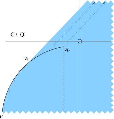
Figure 1: $0<\phi<\frac{\pi}{2}$

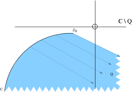
Figure 2: $-\frac{\pi}{2}<\phi\leq 0$

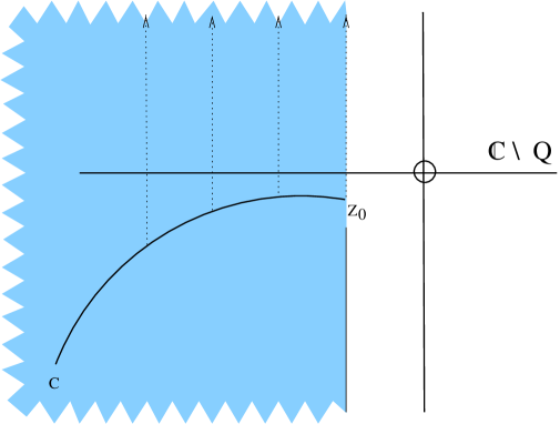
Figure 3: $\phi=\frac{\pi}{2}$

5.2 The classification of $(1.2)$

In this section we analyse the Sims classification of (1. 2) when the coefficients are

$$p(x)=p_{1}x^{a_{1}}+ip_{2}x^{a_{2}},\;q(x)=q_{1}x^{b_{1}}+iq_{2}x^{b_{2}},\;w(x)=x^{\omega},$$ (5. 76)

where $p_{j},q_{j},a_{j},b_{j}\;(j=1,2)$ and $\omega$ are real, and $x\in[1,\infty)$. We write $A={\rm max}\;(a_{1},a_{2})$ and $B={\rm max}\;(b_{1},b_{2},\omega)$. Our results follow from an analysis of the asymptotic behaviour of linearly independent solutions of (1. 2) at infinity as given by the Liouville-Green formulae [3]. A general description covering all cases is far too complicated and hardly helpful. Instead, we provide a prescription for determining the classification. In each specific case the details are straightforward, though tedious.

5.2.1 The case $A-B<2$

In this case, linearly independent solutions $y_{\pm}$ exist which are such that, as $x\rightarrow\infty$

$$y_{\pm}(x)\sim[p(x)s(x)]^{-1/4}\exp\left(\pm\int^{x}_{1}{\rm Re}[(s/p)^{1/2}]dt\right)$$ (5. 77)

$$p(x)y_{\pm}^{{}^{\prime}}(x)\sim[p(x)s(x)]^{1/4}\exp\left(\pm\int^{x}_{1}{\rm Re}[(s/p)^{1/2}]dt\right)$$ (5. 78)

where $s(x)=q(x)-\lambda w(x)$ (see [3, page 58]). We use the notation $f(x)\sim g(x)$ to mean that $f(x)/g(x)\rightarrow 1$ as $x\rightarrow\infty$, and $f(x)\stackrel{{\scriptstyle\smile}}{{\frown}}g(x)$ if $\mid f(x)/g(x)\mid$ is bounded above and below by positive constants. Note that, for $z=re^{i\theta}\;\in{\bf C},\;0\leq\theta<2\pi$, $r>0$, we define the $n^{th}$ root of $z$ to be the complex number $r^{1/n}e^{i\theta/n}$.

Suppose that for some $\Lambda_{\eta,K}$, $(\eta,K)\in S(\alpha)$, and $\lambda\in\Lambda_{\eta,K}$, as $x\rightarrow\infty$,

$${\rm Re}\left[\left(\frac{s(x)}{p(x)}\right)^{1/2}\right]=Dx^{\tau}\left(1+O(\frac{1}{x^{\epsilon}})\right)\;\;\;D\neq 0,\;\epsilon>0,\;\;D,\tau\in{\bf R}$$ (5. 79)

and

$$|p(x)s(x)|\stackrel{{\scriptstyle\smile}}{{\frown}}x^{\gamma}\;\;\gamma\in{\bf R}.$$ (5. 80)

In each of the following cases, at least one of the solutions $y_{+}$ and $y_{-}$ is not in $L^{2}(1,\infty;wdx)$, and hence (1. 2) is in Case I :

1. $\tau>-1$;

2. $\tau=-1$ and $2\mid D\mid+\omega-\gamma/2+1\geq 0$;

3. $\tau<-1$ and $\omega-\gamma/2+1\geq 0$;.

In all other cases when $A-B<2$, and (5. 79), and (5. 80) hold, we are either in Case II or Case III: on setting

$$W_{\pm}(x):={\rm Re}\left[e^{i\eta}\left(p(x)\mid y^{{}^{\prime}}_{\pm}(x)\mid^{2}+s(x)\mid y_{\pm}(x)^{2}\mid\right)\right]$$ (5. 81)

we have that Case III prevails if $W_{+}$ and $W_{-}$ are both integrable (which can be verified using (5. 77) and (5. 78) ) and Case II otherwise.

5.2.2 The case $A-B=2$

In this case the equation (1. 2) is asymptotically of Euler type. Here the results of [3, page 75] give, with $c=1/4(\sqrt{17}-1)$

$$\mid y_{+}\;\mid\stackrel{{\scriptstyle\smile}}{{\frown}}\;x^{2(A-1)c},\;\;\;\mid py_{+}^{{}^{\prime}}\mid\;\stackrel{{\scriptstyle\smile}}{{\frown}}\;x^{2(A-1)(\frac{1}{2}+c)}$$

and

$$\mid y_{-}\mid\;\stackrel{{\scriptstyle\smile}}{{\frown}}x^{-2(A-1)(\frac{1}{2}+c)},\;\;\;\mid py_{-}^{{}^{\prime}}\;\mid\stackrel{{\scriptstyle\smile}}{{\frown}}x^{-2(A-1)c}.$$

At least one of the solutions $y_{+}$, $y_{-}$ is not in $L^{2}(1,\infty;wdx)$, and hence (1. 2) is in Case I, in each of the following cases:

1. $A>1$ and $\omega+4(A-1)c+1\geq 0$;

2. $A=1$ and $\omega\geq-1$;

3. $A<1$ and $\omega-4(A-1)(\frac{1}{2}+c)+1\geq 0$.

In all other cases when $A-B=2$, we are in Case III when $W_{+}$ and $W_{-}$ defined in (5. 81) are both integrable, and Case II otherwise.

5.2.3 The case $A-B>2$

Here the relevant analysis is that in [3, page 78]. It follows that

$$\mid y_{+}\mid\;\stackrel{{\scriptstyle\smile}}{{\frown}}1,\;\;\;\mid y_{+}^{{}^{\prime}}\mid\;\stackrel{{\scriptstyle\smile}}{{\frown}}\;x^{(B-A)/2},$$

$$\mid y_{-}\mid\;\stackrel{{\scriptstyle\smile}}{{\frown}}\;x^{-(A+B)/2},\;\;\;\mid y_{-}^{{}^{\prime}}\mid\;\stackrel{{\scriptstyle\smile}}{{\frown}}\;x^{-A}.$$

At least one of the solutions $y_{+}$,$y_{-}$ is not in $L^{2}(1,\infty;wdx)$, and hence (1. 2) is in Case I, if $\omega-\rm{min}\{0,A+B\}\geq-1$. If $\omega-\rm{min}\{0,A+B\}<-1$, (1. 2) is in Case III if $W_{\pm}$ are both integrable and Case II otherwise.

The case $p=w=1$ is covered in detail in [4, Theorem III, 10.28]; this includes the original example of Sims [9, p. 257] establishing the existence of Case II.

5.3 The spectra

Finally, we investigate the spectra of the operators $\tilde{M}$ generated in $L^{2}(0,\infty)$ by expressions $M$ of the form

$$M[y]=-y^{{}^{\prime\prime}}+cx^{\beta}y,\;\;\;0\leq x<\infty,$$ (5. 82)

where $\beta>0$ and $c\in{\bf C}$ with arg$\;c\in[0,\pi]$; the case arg $c\in(\pi,2\pi)$ is similar.

If arg $c\neq\pi$, we have

$$Q=\{z:0\leq{\rm arg}z\leq{\rm arg}\;c\},\;\;\;Q_{\infty}=\emptyset.$$ (5. 83)

Suppose that

$${\rm Im}[\overline{\sin\alpha}\cos\alpha]\geq 0.$$ (5. 84)

Then, (2. 8) is satisfied for $\eta=-\frac{\pi}{2}$ and, for any $K>0$, $(-\pi/2,K)\in S(\alpha)$. Consequently

$$Q(\alpha)\subseteq{\bf C}\backslash\Lambda_{-\pi/2,K}=\overline{\bf C_{+}}$$ (5. 85)

and, similarly,

$$Q_{\infty}(\alpha)=\emptyset$$ (5. 86)

(see (3. 42)). Also, it follows from Section 5.2.1 (item 1) that Case I holds. Hence, by Theorem 4.7 and Remark 4.8, for arg $c\neq\pi$, the operator realisation $\tilde{M}$ of $M$ defined in (4. 55) has empty essential spectrum $\sigma_{e}(\tilde{M})$. Such a result is given in [5, Theorem 30] for the analogous problem on $(-\infty,\infty)$.

If arg $c=\pi$, we have

$$Q=Q_{\infty}={\bf R}$$ (5. 87)

and, if (5. 84) is satisfied, $Q(\alpha)\subseteq({\bf C}\backslash\Lambda_{-\pi/2,K})\cap({\bf C}\backslash\Lambda_{\pi/2,K})={\bf R}$, and hence

$$Q(\alpha)=Q_{\infty}(\alpha)={\bf R}.$$ (5. 88)

For $\lambda=i$ and $\eta=\pm\pi/2$, we now have $\mid W_{\pm}\mid=\mid y_{\pm}\mid^{2}$ and in Section 5.2.1

$$y_{\pm}(x)\stackrel{{\scriptstyle\smile}}{{\frown}}\left\{\begin{array}[]{cc}x^{-\beta/4}&{\rm if\;}\beta>2,\\ x^{-\frac{1}{2}\mp\frac{1}{2\mid c\mid^{1/2}}}&{\rm if\;}\beta=2,\\ x^{-\frac{\beta}{4}}exp[\mp\frac{x^{1-\beta/2}}{\mid c\mid^{1/2}(2-\beta)}]&{\rm if\;}\beta<2.\end{array}\right.$$

It follows that Case I holds if $\beta\leq 2$ and Case III if $\beta>2$; note that Case III is now the Weyl limit-circle case since $M$ is formally symmetric. Hence, if arg $c=\pi$, by Theorem 4.5,

$$\sigma_{e}(\tilde{M})\left\{\begin{array}[]{cc}=\emptyset&{\rm if\;}\beta>2,\\ \subseteq{\bf R}&{\rm if\;}\beta\leq 2.\end{array}\right.$$ (5. 89)

If $\alpha$ is real, (5. 84) is satisfied. In this case, when $\beta\leq 2$, $M$ is in the Weyl limit-point case at $\infty$ (so that $\tilde{M}$ is self-adjoint) and $\sigma_{e}(\tilde{M})={\bf R}$ (see [11, Theorem V.5.10]).

In Case I the identity (5. 90) below (which holds for (1. 2) in general) is often useful and reinforces Remark 4.8. Denote the functions $\theta,\;\phi$ in (2. 10) by $\theta_{\alpha},\;\phi_{\alpha}$ respectively, and the corresponding $m-$function by $m_{\alpha}$. Since $\alpha=0,\pi/2$ satisfy (2. 8) for any $\eta$, we have $Q(0)=Q(\pi/2)=Q$. Also, for $\lambda\not\in Q(\alpha)$, there exist $K\neq 0$ such that

$$\theta_{\alpha}(x,\lambda)+m_{\alpha}(\lambda)\phi_{\alpha}(x,\lambda)=K[\theta_{\pi/2}(x,\lambda)+m_{\pi/2}(\lambda)\phi_{\pi/2}(x,\lambda)].$$

On substituting (2. 10) we have

$$m_{\alpha}(\lambda)=\frac{m_{\pi/2}(\lambda)\sin\alpha-\cos\alpha}{m_{\pi/2}(\lambda)\cos\alpha+\sin\alpha}.$$ (5. 90)

Hence, if $m_{\pi/2}$ is meromorphic in ${\bf C}$, the same is true of $m_{\alpha}$, for any $\alpha$.

An important special case of (5. 82) is the expression for the harmonic oscillator

$$M[y]=-y^{{}^{\prime\prime}}+cx^{2}y\;\;\;\;0\leq x<\infty.$$

On setting $x=\frac{z}{\sqrt{2}c^{1/4}}$, the equation $(M-\lambda)[y]=0$ becomes

$$-y^{{}^{\prime\prime}}+\frac{1}{4}z^{2}y=\mu y$$ (5. 91)

where ^′ now denotes differentiation with respect to $z$ along the ray with argument $\frac{1}{4}{\rm arg}\;c$, and $\mu=\frac{\lambda}{2\sqrt{c}}$. From [12, page 341], for $0\leq{\rm arg}c<\pi$, the unique solution of (5. 91) in $L^{2}(0,\infty)$ is the parabolic cylinder function $D_{\mu-1/2}(z)$. It follows from (2. 10) and the fact that our function $\psi$ in (2. 24) must be a constant multiple of $D_{\mu-1/2}(z)$ that

$$m_{\pi/2}(\lambda)=\frac{D_{\mu-1/2}(0)}{D^{{}^{\prime}}_{\mu-1/2}(0)}$$

and this gives

$$m_{\pi/2}(\lambda)=-\frac{1}{2c^{1/4}}\frac{\Gamma(1/4-\frac{\lambda}{4\sqrt{c}})}{\Gamma(3/4-\frac{\lambda}{4\sqrt{c}})}.$$ (5. 92)

This is meromorphic with poles at

$$\lambda_{n}=(4n+1)\sqrt{c},\;\;\;n=0,1,2,...$$

When arg $c=\pi$, $Q=Q_{\infty}={\bf R}$, and for $\alpha=\pi/2$, there are $m$-functions defined in ${\bf C_{+}}$ and ${\bf C_{-}}$ :

$$m^{(1)}_{\pi/2} = -\frac{e^{-i\pi/4}}{2\mid c\mid^{1/4}}\frac{\Gamma(1/4-\frac{\lambda}{4\sqrt{c}})}{\Gamma(3/4-\frac{\lambda}{4\sqrt{c}})}\;\;\;(\lambda\in{\bf C_{+}})$$

$$m^{(2)}_{\pi/2} = -\frac{e^{i\pi/4}}{2\mid c\mid^{1/4}}\frac{\Gamma(1/4+\frac{\lambda}{4\sqrt{c}})}{\Gamma(3/4+\frac{\lambda}{4\sqrt{c}})}\;\;\;(\lambda\in{\bf C_{-}});$$

${\bf C_{+}},{\bf C_{-}}$ are the connected components $C_{1},C_{2}$ referred to in Lemma 3.1 and the following comment. These functions are not analytic continuations of each other and the self adjoint operator $\tilde{M}$, with $\alpha=\pi/2$, has $\sigma_{e}(\tilde{M})={\bf R}$: this is therefore true for all values of $\alpha$ by Remark 4.8. Criteria on $q$ for $\sigma_{e}(\tilde{M})\supseteq[0,\infty)$ in the case $p=w=1$ are given in [6]; see also [5, Chapter VII].

References

• [1] E. S. Birger and G. A. Kalyabin. The theory of Weyl limit-circles in the case of non-self-adjoint second-order differential-equation systems. Differentsial’nye Uravneniya, 12, no 9, 1531–1540, 1976. English translation: Differential Equations 12, no 9, 1077-1084 (1977).
• [2] J. Chaudhuri and W. N. Everitt. On the spectrum of ordinary second-order differential operators. Proc. Roy. Soc. Edin., A(68):95–119, 1968.
• [3] M. S. P. Eastham. The Asymptotic Solution of Linear Differential Systems. L.M.S. Monograph 4. Oxford, 1989.
• [4] D. E. Edmunds and W. D. Evans. Spectral Theory and Differential Operators. Oxford University Press, 1987.
• [5] I. M. Glazman. Direct Methods of Qualitative Spectral Analysis of Singular Differential Operators. Israel program for scientific translations Ltd. Jerusalem, 1965.
• [6] Y. Kamimura. On the spectrum of an ordinary differential operator with an $r$-integrable complex-valued potential. J. London Math. Soc. (2), 20:86–100, 1979.
• [7] T. Kato. Perturbation Theory for Linear Operators, (2nd edition). Springer-Verlag, Berlin, Heidelberg, New York, 1976.
• [8] J. B. McLeod. Eigenfunction expansions associated with a complex differential operator of the second order. Quart. J. Math. Oxford (2), 12:291–303, 1961.
• [9] A. R. Sims. Secondary conditions for linear differential operators of the second order. J. of Mathematics and Mechanics, 6:247–285, 1957.
• [10] E. C. Titchmarsh. Eigenfunction Expansions Part II. Clarendon Press, Oxford, 1958.
• [11] E. C. Titchmarsh. Eigenfunction Expansions Part I, (2nd edition). Clarendon Press, Oxford, 1962.
• [12] E. T. Whittaker and G. N. Watson. A Course of Modern Analysis, (2nd edition). Cambridge University Press, 1915.