Rational rays and Critical portraits of complex polynomials

Stony Brook IMS Preprint #1997/15 October 1997

Introduction

Since external rays were introduced by Douady and Hubbard [DH1] they have played a key role in the study of the dynamics of complex polynomials. The pattern in which external rays approach the Julia set allow us to investigate its topology and to point out similarities and differences between distinct polynomials. This pattern can be organized in the form of “combinatorial objects”. One of these combinatorial objects is the rational lamination.

The rational lamination ${\lambda_{{\mathbb{Q}}}}(f)$ of a polynomial $f$ with connected Julia set $J(f)$ captures how rational external rays land. More precisely, the rational lamination ${\lambda_{{\mathbb{Q}}}}(f)$ is an equivalence relation in ${{\mathbb{Q}}/{\mathbb{Z}}}$ which identifies two arguments $t$ and $t^{\prime}$ if and only if the external rays with arguments $t$ and $t^{\prime}$ land at a common point (compare [McM]).

The aim of this work is to describe the equivalence relations in ${{\mathbb{Q}}/{\mathbb{Z}}}$ that arise as the rational lamination of polynomials with all cycles repelling. We also describe where in parameter space one can find a polynomial with all cycles repelling and a given rational lamination. At the same time we derive some consequences that this study has regarding the topology of Julia sets.

To simplify our discussion let us assume, for the moment, that all the polynomials in question are monic and that they have connected Julia sets.

Now let us summarize our results. A more detailed discussion can be found in the introduction to each Chapter. We start with the results regarding the topology of Julia sets.

Under the assumption that all the cycles of $f$ are repelling, the Julia set $J(f)$ is a full, compact and connected set which might be locally connected or not. If the Julia set $J(f)$ is locally connected then the rational lamination ${\lambda_{{\mathbb{Q}}}}(f)$ completely determines the topology of $J(f)$ and the topological dynamics of $f$ on $J(f)$ (see Proposition 11.4). When the Julia set $J(f)$ is not locally connected it is meaningful to study its topology via prime end impressions. We show that each point in $J(f)$ is contained in at least one and at most finitely many prime end impressions. Also, we show that $J(f)$ is locally connected at periodic and pre-periodic points of $f$:

Theorem 1.

Consider a polynomial $f$ with connected Julia set $J(f)$ and all cycles repelling.

(a) If $z$ is a periodic or pre-periodic point then $J(f)$ is locally connected at z. Moreover, if a prime end impression $Imp\subset J(f)$ contains $z$ then the prime end impression $Imp$ is the singleton $\{z\}$.

(b) For an arbitrary $z\in J(f)$, $z$ is contained in at least one and at most finitely many prime end impressions.

Roughly, part (a) of the previous Theorem is a consequence of the fact that the rational lamination ${\lambda_{{\mathbb{Q}}}}(f)$ of a polynomial $f$ with all cycles repelling is abundant in non-trivial equivalence classes. As a matter of fact we will show that ${\lambda_{{\mathbb{Q}}}}(f)$ is maximal with respect to some simple properties. Part (b) of the previous Theorem is ultimately a consequence of the following result which generalizes one by Thurston for quadratic polynomials (see [Th]):

Theorem 2.

Consider a point $z$ in the connected Julia set $J(f)$ of a polynomial $f$ of degree $d$. Provided that $z$ has infinite forward orbit, there are at most $2^{d}$ external rays landing at $z$. Moreover, for $n$ sufficiently large, there are at most $d$ external rays landing at $f^{\circ n}(z)$.

As mentioned before, we describe which equivalence relations in ${{\mathbb{Q}}/{\mathbb{Z}}}$ are the rational lamination ${\lambda_{{\mathbb{Q}}}}(f)$ of a polynomial $f$ with all cycles repelling. The description will be in terms of critical portraits. Critical portraits were introduced by Fisher in [F] to capture the location of the critical points of critically pre-repelling maps and since then extensively used in the literature (see [BFH, GM, P, G]). A critical portrait is a collection ${\Theta}=\{{\Theta}_{1},\dots\Theta_{m}\}$ of finite subsets of ${{\mathbb{R}}/{\mathbb{Z}}}$ that satisfy three properties:

$\bullet$ For every $j$, $|\Theta_{j}|\geq 2$ and $|d\cdot\Theta_{j}|=1$,

$\bullet$ $\Theta_{1},\dots,\Theta_{m}$ are pairwise unlinked,

$\bullet$ $\sum(|\Theta_{j}|-1)=d-1$.

Motivated by the work of Bielefield, Fisher and Hubbard [BFH], each critical portrait ${\Theta}$ generates an equivalence relation ${\Lambda_{{\mathbb{Q}}}}({\Theta})$ in ${{\mathbb{Q}}/{\mathbb{Z}}}$. The idea is that each critical portrait ${\Theta}$ determines a partition of the circle into $d$ subsets of lenght $1/d$ which we call ${\Theta}$-unlinked classes. Symbolic dynamics of multiplication by $d$ in ${{\mathbb{R}}/{\mathbb{Z}}}$ gives rise to an equivalence relation ${\Lambda_{{\mathbb{Q}}}}({\Theta})$ in ${{\mathbb{Q}}/{\mathbb{Z}}}$ which is a natural candidate to be the rational lamination of a polynomial. A detailed discussion of this construction is given in Chapter 4 where we make a fundamental distinction between critical portraits. That is, we distinguish between critical portraits with “periodic kneading” and critical portraits with “aperiodic kneading”. We show that critical portraits with aperiodic kneading correspond to rational laminations of polynomials with all cycles repelling:

Theorem 3.

Consider an equivalence relation ${\lambda_{{\mathbb{Q}}}}$ in ${{\mathbb{Q}}/{\mathbb{Z}}}$. ${\lambda_{{\mathbb{Q}}}}$ is the rational lamination ${\lambda_{{\mathbb{Q}}}}(f)$ of some polynomial $f$ with connected Julia set and all cycles repelling if and only if ${\lambda_{{\mathbb{Q}}}}={\Lambda_{{\mathbb{Q}}}}({\Theta})$ for some critical portrait ${\Theta}$ with aperiodic kneading.

Moreover, when the above holds, there are at most finitely many critical portraits ${\Theta}$ such that ${\lambda_{{\mathbb{Q}}}}={\Lambda_{{\mathbb{Q}}}}({\Theta})$.

In the previous Theorem, the fact that every rational lamination is generated by a critical portrait is consequence of the study of rational laminations discussed in Chapter 3. The existence of a polynomial with a given rational lamination relies on finding a polynomial in parameter space with the desired rational lamination. Alternatively, the results of [BFH] can be used to give a simpler proof of Theorem 3. We will not do this here.

In parameter space, following Branner and Hubbard [BH], we work in the space ${{\mathcal{P}}_{d}}$ of monic centered polynomials of degree $d$. That is, polynomials of the form:

$$z^{d}+a_{d-2}z^{d-2}+\cdots+a_{0}.$$

The set of polynomials $f$ in ${{\mathcal{P}}_{d}}$ with connected Julia set $J(f)$ is called the connectedness locus ${{\mathcal{C}}_{d}}$. We search for polynomials in ${{\mathcal{C}}_{d}}$ by looking at ${{\mathcal{C}}_{d}}$ from outside. Of particular convenience for us is to explore the shift locus ${{\mathcal{S}}_{d}}$. The shift locus ${{\mathcal{S}}_{d}}$ is the open, connected and unbounded set of polynomials $f$ such that all critical points of $f$ escape to infinity. The shift locus ${{\mathcal{S}}_{d}}$ is the unique hyperbolic component in parameter space formed by polynomials with all cycles repelling. We will concentrate in the set $\partial{{\mathcal{S}}_{d}}\cap{{\mathcal{C}}_{d}}$ where the shift locus ${{\mathcal{S}}_{d}}$ and the connectedness locus ${{\mathcal{C}}_{d}}$ “meet”. Conjecturally, every polynomial with all cycles repelling and connected Julia set lies in $\partial{{\mathcal{S}}_{d}}\cap{{\mathcal{C}}_{d}}$.

To describe where in parameter space we can find a polynomial with a given rational lamination, in Chapter 2, we cover $\partial{{\mathcal{S}}_{d}}\cap{{\mathcal{C}}_{d}}$ by smaller dynamically defined sets that we call the “impressions of critical portraits”. More precisely, inspired by Goldberg [G], we show that each critical portrait ${\Theta}$ naturally defines a direction to go from the shift locus ${{\mathcal{S}}_{d}}$ to the connected locus ${{\mathcal{C}}_{d}}$. Loosely, the set of polynomials in $\partial{{\mathcal{S}}_{d}}\cap{{\mathcal{C}}_{d}}$ reached by a given direction ${\Theta}$ is called the impression $I_{{{\mathcal{C}}_{d}}}({\Theta})\subset{{\mathcal{C}}_{d}}$ of the critical portrait ${\Theta}$. Each critical portrait impression is a closed connected subset of $\partial{{\mathcal{S}}_{d}}\cap{{\mathcal{C}}_{d}}$ and the set of all impressions covers all of $\partial{{\mathcal{S}}_{d}}\cap{{\mathcal{C}}_{d}}$. It is worth to point out that, for quadratic polynomials, there is a one to one correspondence between prime end impression of the Mandelbrot set and impressions of quadratic critical portraits.

We characterize the impressions that contain polynomials with all cycles repelling and a given rational lamination:

Theorem 4.

Consider a map $f$ in the impression $I_{{{\mathcal{C}}_{d}}}({\Theta})\subset{{\mathcal{C}}_{d}}$ of a critical portrait ${\Theta}$.

If ${\Theta}$ has aperiodic kneading then ${\lambda_{{\mathbb{Q}}}}(f)={\Lambda_{{\mathbb{Q}}}}({\Theta})$ and all the cycles of $f$ are repelling.

If ${\Theta}$ has periodic kneading then at least one cycle of $f$ is non-repelling.

The previous Theorem leads to a new proof of the Bielefield-Fisher-Hubbard realization Theorem for critically pre-repelling maps [BFH]. This proof replaces the use of Thurston’s characterization of post-critically finite maps [DH2] with parameter space techniques. The parameter space techniques shed some light on how polynomials are distributed in $\partial{{\mathcal{S}}_{d}}\cap{{\mathcal{C}}_{d}}$ according to their combinatorics.

For quadratic polynomials, the results previously stated are well known, sometimes in a different but equivalent language (see [DH1, Th, La, At, D, McM, Sch, M2]). Also, the Mandelbrot Local Connectivity Conjecture states that quadratic impressions are singletons. For higher degrees, we do not expect this to be true. That is, we conjecture the existence non-trivial impressions of critical portraits with aperiodic kneading.

This work is organized as follows:

In Chapter 1, we study external rays that land at a common point. Namely, following Goldberg and Milnor, the type $A(z)$ of a point $z$ and the orbit portrait $A({\mathcal{O}})$ of an orbit ${\mathcal{O}}$ are introduced. Their basic properties are discussed and applied to prove Theorem 2.

In Chapter 2, we cover $\partial{{\mathcal{S}}_{d}}\cap{{\mathcal{C}}_{d}}$ by critical portrait impressions. Here, the main issue is to overcome the nontrivial topology that the shift locus has for degrees greater than two [BDK]. Inspired by Goldberg we do so by restricting our attention to a dense subset of the shift locus that we call the visible shift locus. In the visible shift locus one can introduce coordinates by means of critical portraits. Then, after endowing the set of critical portraits with the compact-unlinked topology, it is not difficult to define critical portrait impressions. In this Chapter, we also discuss the pattern in which external rays of polynomials in the visible shift locus land (see Section 8). This discussion, although elementary, plays a key role in the next two Chapters.

In Chapter 3, we discuss the basic properties of rational laminations and at the same time we proof Theorem 1. On one hand part (a) of this Theorem relies on working with puzzle pieces. On the other, we deduce part (b) of Theorem 1 from Theorem 2. This argument makes use of an auxiliary polynomial in the visible shift locus. That is, we profit from the fact that, for polynomials in the visible shift locus, the pattern in which external rays land is transparent.

In Chapter 4, we show how each critical portrait ${\Theta}$ gives rise to an equivalence relation ${\Lambda_{{\mathbb{Q}}}}({\Theta})$ in ${{\mathbb{Q}}/{\mathbb{Z}}}$ and proceed to collect threads from Chapters 2 and 3 to prove Theorems 3 and 4.

Acknowledgments: This work is a copy of the author’s Ph. D. Thesis. I am grateful to Jack Milnor for his enlightening comments and suggestions as well as for his support and good advise. I am grateful to Misha Lyubich for his insight and questions and to Alfredo Poirier for explaining me his work. This work was partially supported by a “Beca Presidente de la Repúblic” (Chile).

Chapter 1: Orbit Portraits

1. Introduction

The main purpose of this chapter is to study external rays that land at a common point in the Julia set $J(f)$ of a polynomial $f$. The main result here is to give an upper bound on the number of external rays that can land at a point with infinite forward orbit.

For quadratic polynomials, it follows from Thurston’s work on quadratic laminations that at most 4 rays can land at a point $z$ with infinite forward orbit. Moreover, all but finitely many forward orbit elements are the landing point of at most 2 rays (see [Th] Gaps eventually cycle). Here we generalize this result:

Theorem 1.1.

Let $f$ be a degree $d$ monic polynomial with connected Julia set $J(f)$. If $z\in J(f)$ is a point with infinite forward orbit then at most $2^{d}$ external rays can land at $z$. Moreover, for $n$ sufficiently large, at most $d$ external rays can land at $f^{\circ n}(z)$.

Although our main interest is the finiteness given by this result, we should comment on the bounds obtained. For quadratic polynomials both bounds are sharp and due to Thurston. For higher degree polynomials, we expect $2^{d}$ to be optimal in the statement of the Theorem (see Figure 1). But we do not know if there is an infinite orbit of a cubic polynomial with exactly $3$ external rays landing at each orbit element.

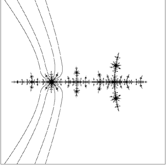
Figure 1. The Julia set of the cubic polynomial $f(z)=z^{3}-1.743318z+0.50322$ with eight rays “landing” at the critical point $c_{-}=-0.581106$.

The main ingredients in the proof of Theorem 1.1 are the ideas and techniques introduced by Goldberg and Milnor [GM, M2] to study external rays that land at a common point $z$ i.e. “the type of $z$”.

This Chapter is organized as follows:

In Section 2, we recall some results from polynomial dynamics. For further reference see [M1, CG].

In Sections 3 and 4, following Goldberg and Milnor [GM], orbit portraits are introduced and some of their basic properties are discussed.

In Section 5, we apply these properties to obtain bounds on the number of cycles participating in a periodic orbit portrait. Also, this illustrates some of the ideas involved in the proof of Theorem 1.1.

In Section 6, we prove Theorem 1.1.

2. Preliminaries

Here we recall some facts about polynomial dynamics. For more background material we refer the reader to [M1].

Consider a monic polynomial $f:{\mathbb{C}}\rightarrow{\mathbb{C}}$ of degree $d$. Basic tools to understand the dynamics of $f$ are the Green function $g_{f}$ and the Böttcher map $\phi_{f}$.

The Green function $g_{f}$ measures the escape rate of points to $\infty$:

$$\begin{array}[]{lccl}g_{f}:&{\mathbb{C}}&\rightarrow&{{\mathbb{R}}}_{\geq 0}\\ &z&\mapsto&\lim\frac{\log_{+}|f^{\circ n}(z)|}{d^{n}}\\ \end{array}$$

It is a well defined continuous function which vanishes on the filled Julia set $K(f)$ and satisfies the functional relation:

$$g_{f}(f(z))=dg_{f}(z).$$

Moreover, $g_{f}$ is positive and harmonic in the basin of infinity $\Omega(f)$. In $\Omega(f)$, the derivative of $g_{f}$ vanishes at $z$ if and only if $z$ is a pre-critical point of $f$. In order to avoid confusions, we say that $z$ is a singularity of $g_{f}$.

The Böttcher map $\phi_{f}$ conjugates $f$ with $z\mapsto z^{d}$ in a neighbourhood of $\infty$. The germ of $\phi_{f}$ at $\infty$ is unique up to conjugacy by $z\mapsto\zeta z$ where $\zeta$ is a $(d-1)st$ root of unity. Since $f$ is monic we can normalize $\phi_{f}$ to be asymptotic to the identity:

$$\frac{\phi_{f}(z)}{z}\rightarrow 1$$

as $z\rightarrow\infty$. Observe that near infinity, $g_{f}(z)=\log|\phi_{f}(z)|$.

For the purpose of simplicity, we make a distinction according to whether the Julia set $J(f)$ is connected or disconnected.

2.1. Connected Julia sets

The Julia set $J(f)$ is connected if and only if all the critical points of $f$ are non-escaping. That is, the forward orbit of the critical points remains bounded. Thus, $g_{f}$ has no singularities in $\Omega(f)$. Moreover, the Böttcher map extends to the basin of infinity $\Omega(f)$,

$$\phi_{f}:\Omega(f)\rightarrow{{\mathbb{C}}\setminus\overline{{\mathbb{D}}}}$$

and $\phi_{f}(f(z))=(\phi_{f}(z))^{d}$ for $z\in\Omega(f)$. Furthermore,

$$g_{f}(z)=\log_{+}|\phi_{f}(z)|\mbox{ for }z\in\Omega(f).$$

An external ray $R^{t}_{f}$ is the pre-image of radial line $(1,\infty)e^{2\pi it}$ under $\phi_{f}$, i.e.

$$R^{t}_{f}=\phi^{-1}_{f}((1,\infty)e^{2\pi it}).$$

Thus, external rays are curves that run from infinity towards the Julia set $J(f)$. If $R^{t}_{f}$ has a well defined limit $z\in J(f)$ as it approaches the Julia set $J(f)$ we say that $R^{t}_{f}$ lands at $z$.

External rays are parameterized by the circle ${{\mathbb{R}}/{\mathbb{Z}}}$ and $f$ acts on external rays as multiplication by $d$. (i.e. $f(R^{t}_{f})=R^{dt}_{f}$ ). A ray $R^{t}_{f}$ is said to be rational if $t\in{{\mathbb{Q}}/{\mathbb{Z}}}$. Rational rays can be either periodic or pre-periodic according to whether $t$ is periodic or pre-periodic under $m_{d}:t\mapsto dt$. A periodic ray always lands at a repelling or parabolic periodic point. A pre-periodic ray lands at a pre-repelling or pre-parabolic point [DH1]. Conversely, putting together results of Douady, Hubbard, Sullivan and Yoccoz [H, M1], we have the following:

Theorem 2.1.

Let $z$ be a parabolic or repelling periodic point in a connected Julia set $J(f)$. Then there exists at least one periodic ray landing at $z$. Moreover, all the rays that land at $z$ are periodic of the same period.

2.2. Disconnected Julia sets

A polynomial $f$ has disconnected Julia set $J(f)$ if and only if some critical point of $f$ lies in the basin of infinity $\Omega(f)$. In this case, the Böttcher map does not extend to all of $\Omega(f)$. It extends, along flow lines, to the basin of infinity under the gradient flow $\mathrm{grad}g_{f}$. Following Levin and Sodin [LS], the reduced basin of infinity $\Omega^{*}(f)$ is the basin of infinity under the gradient flow $\mathrm{grad}g_{f}$. Now

$$\phi_{f}:\Omega^{*}(f)\rightarrow U_{f}\subset{{\mathbb{C}}\setminus\overline{{\mathbb{D}}}}$$

is a conformal isomorphism from $\Omega^{*}(f)$ onto a starlike (around $\infty$) domain $U_{f}$. A flow line of $\mathrm{grad}g_{f}$ in $\Omega^{*}(f)$ is an external radius. An external radius maps into an external radius by $f$. Thus, $f(\Omega^{*}(f))\subset\Omega^{*}(f)$.

External radii are parameterized by ${{\mathbb{R}}/{\mathbb{Z}}}$. More precisely, for $t\in{{\mathbb{R}}/{\mathbb{Z}}}$ let $(r,\infty)e^{2\pi it}$ be the maximal portion of $(1,\infty)e^{2\pi it}$ contained in $U_{f}$. The external radius $R^{*t}_{f}$ with argument $t$ is

$$R^{*t}_{f}=\phi^{-1}_{f}((r,\infty)e^{2\pi it}).$$

As one follows the external radius $R^{*t}_{f}$ from $\infty$ towards the Julia set $J(f)$ one might hit a singularity $z$ of $g_{f}$ or not. In the first case, $r>1$ and we say that $R^{*t}_{f}$ terminates at $z$. In the second case, $r=1$ and $R^{*t}_{f}$ is in fact the smooth external ray $R^{t}_{f}$ with argument $t$. Notice that, from the point of view of the gradient flow, an external radius which terminates at a singularity $z$ is an unstable manifold of $z$.

Under iterations of $f$, each point $z$ in the basin of infinity $\Omega(f)$ eventually maps to a point in the reduced basin of infinity $\Omega^{*}(f)$. Say that $f^{\circ n}(z)\in\Omega^{*}(f)$ and that the local degree of $f^{\circ n}$ at $z$ is $k$. After a conformal change of coordinates, the gradient flow lines nearby $z$ are the pre-image under $w\mapsto w^{k}$ of the horizontal flow lines near the origin. Thus, at a singularity $z$ of $g_{f}$, there are exactly $k$ local unstable and $k$ local stable manifolds which alternate as one goes around $z$. A local unstable manifold is contained in $\Omega^{*}(f)$ if and only if it is part of an external radius that terminates at $z$.

Now let $\theta_{1},\dots,\theta_{l}$ be the arguments of the external radii that terminate at critical points of $f$. Since every pre-critical point of $f$ is a singularity of $g_{f}$, the external radii with arguments in

$$\Sigma=\bigcup_{n\geq 0}m^{-n}_{d}(\{\theta_{1},\dots,\theta_{l}\})$$

also terminate at a singularities. Since every singularity is a pre-critical point we have smooth external rays defined for arguments in ${{\mathbb{R}}/{\mathbb{Z}}}\setminus\Sigma$. Following Goldberg and Milnor, for $t\in{{\mathbb{R}}/{\mathbb{Z}}}$ let

$$R^{t^{\pm}}_{f}=\lim_{s\rightarrow t^{\pm}}R^{s}_{f}.$$

If $t\notin\Sigma$ then $R^{t^{\pm}}_{f}$ coincide, and we say that $R^{t}_{f}$ is a smooth external ray. If $t\in\Sigma$ then $R^{t^{\pm}}_{f}$ do not agree, and we say that they are non-smooth or bouncing rays with argument $t$.

Notice that $f(R^{t^{\epsilon}}_{f})=R^{dt^{\epsilon}}_{f}$. We say that $R^{t^{\epsilon}}_{f}$ is periodic or pre-periodic if $t$ is periodic or pre-periodic under $m_{d}:t\mapsto dt$. Here, we also have that periodic rays land at repelling or parabolic periodic points. But, there might be rays, which are not periodic, landing at a periodic point $z$. Following Levin and Przyticky [LP], the landing Theorem stated for connected Julia sets generalizes to:

Theorem 2.2.

Let $z$ be a repelling or parabolic periodic point. Then there exists at least one external ray landing at $z$. Moreover,

Either all the external rays, smooth and non-smooth, landing at $z$ are periodic of the same period,

Or, the arguments of the external rays, smooth and non-smooth, landing at $z$ are irrational and form a Cantor set. Furthermore, $\{z\}$ is a connected component of $J(f)$ and there are non-smooth rays landing at $z$.

3. Orbit Portraits

We fix, for this Chapter, a monic polynomial $f$ of degree $d$ with Julia set $J(f)$ (possibly disconnected). Our goal is to study external rays that land at a common point:

Definition 3.1.

Consider a point $z\in J(f)$. Suppose that at least one external ray lands at $z$ and that all the external rays which land at $z$ are smooth. We say that

$$A(z)=\{t\in{{\mathbb{R}}/{\mathbb{Z}}}:R^{t}_{f}\mbox{ lands at }z\}$$

is the type of $z$.

Let ${\mathcal{O}}=\{z,f(z),\dots\}$ be the forward orbit of $z$, we say that

$$A({\mathcal{O}})=\{A(w):w\in{\mathcal{O}}\}$$

is the orbit portrait of ${\mathcal{O}}$. In particular, when ${\mathcal{O}}$ is a periodic cycle we say that $A({\mathcal{O}})$ is a periodic orbit portrait.

Figure 2 shows the external rays landing at a period 3 orbit ${\mathcal{O}}$ of a cubic polynomial with orbit portrait $A({\mathcal{O}})$:

$$\{\{2/26,10/26,19/26\},\{4/26,5/26,6/26\},\{12/26,15/26,18/26\}\}.$$

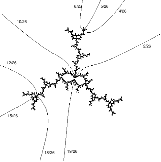
Figure 2. External rays landing at a period 3 orbit of a cubic polynomial.

Remark: Below we will see that if the type $A(z)$ of $z$ is well defined then the type $A(f(z))$ is also well defined (Lemma 3.3).

Theorem 1.1 follows from the slightly more general:

Theorem 3.2.

Consider a monic polynomial $f$ of degree $d$ with Julia set $J(f)$. If $A(z)$ is the type of a Julia set element $z$ with infinite forward orbit then the cardinality of $A(z)$ is at most $2^{d}$. Moreover, for $n$ sufficiently large, the cardinality of $A(f^{\circ n}(z))$ is at most $d$.

Remark: Above, in the statement of Theorem, we do not assume that the Julia set is connected because, in Chapter 3, we will need to apply this result for polynomials with disconnected Julia set.

Now we list the basic properties of types, proofs are provided at the end of this section. Recall that $m_{d}:t\rightarrow dt$ denotes multiplication by $d$ modulo $1$.

Types are invariant under dynamics:

Lemma 3.3.

If $A(z)$ is the type of $z$ then $A(f(z))=m_{d}(A(z))$. Moreover, ${m_{d}}_{|A(z)}$ is a $k$ to $1$ map where $k$ is the local degree of $f$ at $z$.

Provided that $z$ is not a critical point, the transition from the type of $z$ to that of its image $f(z)$ is cyclic order preserving:

Lemma 3.4.

If $z$ is not a critical point of $f$ then

$${{m_{d}}_{|}}_{A(z)}:A(z)\rightarrow A(f(z))$$

is a cyclic order preserving bijection.

Often we study types of several points at the same time. Since smooth external rays are disjoint, types of distinct points embed in ${{\mathbb{R}}/{\mathbb{Z}}}$ in an “unlinked” fashion.

Lemma 3.5.

If $A(z)$ and $A(\hat{z})$ are distinct types then $A(z)$ is contained in a connected component of ${{\mathbb{R}}/{\mathbb{Z}}}\setminus A(\hat{z})$.

Definition 3.6.

We say that two subsets $A,A^{\prime}\subset{{\mathbb{R}}/{\mathbb{Z}}}$ are unlinked if and only if $A$ is contained in a connected component of ${{\mathbb{R}}/{\mathbb{Z}}}\setminus A^{\prime}$.

While types live in ${{\mathbb{R}}/{\mathbb{Z}}}$, external rays are contained in the complex plane ${\mathbb{C}}$. It is convenient to have both objects in the same topological space:

Definition 3.7.

The circled plane $\copyright$ is the closed topological disk obtained by adding to ${\mathbb{C}}$ a circle of points $\lim_{r\rightarrow\infty}re^{2\pi it}$ at infinity. The boundary $\partial\copyright$ is canonically identified with ${{\mathbb{R}}/{\mathbb{Z}}}$.

Thus, a type $A(z)$ can be considered as a subset of ${{\mathbb{R}}/{\mathbb{Z}}}\cong\partial\copyright$ and the external rays landing at $z$ are arcs that join $A(z)\subset\partial\copyright$ with $z$.

Now we proceed to prove the Lemmas stated above. But before, let us fix the standard orientation in ${{\mathbb{R}}/{\mathbb{Z}}}$ and use interval notation accordingly with the agreement that the interval $(t,t)$ represents the circle ${{\mathbb{R}}/{\mathbb{Z}}}$ with the point $t$ removed.

Proof of Lemma 3.3: If $t\in A(z)$ then the external ray $R^{t}_{f}$ lands at $z$. Continuity of $f$ plus the fact that $f(R^{t}_{f})=R^{dt}_{f}$ assures that $dt\in A(f(z))$. Conversely, if $s\in A(f(z))$ then, locally around $z$, the preimage of $R^{s}_{f}$ is formed by $k$ arcs. Each of these arcs must belong to a smooth external ray because in the definition of $A(z)$ we assume that all the external rays landing at $z$ are smooth. $\Box$

Proof of Lemma 3.4: Since $f$ is locally orientation preserving around $z$ it must preserve the cyclic order of the rays landing at $z$. $\Box$

Proof of Lemma 3.5: By contradiction, assume that $\{\hat{s},\hat{s}^{\prime}\}\subset A(\hat{z})$ and $\{s,s^{\prime}\}\subset A(z)$ are such that $\hat{s}\in(s,s^{\prime})$ and $\hat{s}^{\prime}\in(s^{\prime},s)$. Then the rays $R^{s}_{f}$, $R^{s^{\prime}}_{f}$ together with $z$ chop the complex plane ${\mathbb{C}}$ into two connected components. One which contains $R^{\hat{s}}_{f}$ and another which contains $R^{\hat{s}^{\prime}}_{f}$. Thus $\hat{z}$ lies in two different sets. Contradiction. $\Box$.

4. Sectors

We want to count the number of external rays that participate in some types. Following Goldberg and Milnor [GM, M2], several counting problems can be tackled by a detailed study of the partitions of ${\mathbb{C}}$ and ${{\mathbb{R}}/{\mathbb{Z}}}$ which arise from a given type. To obtain useful information we work under the assumption that there are finitely many elements participating in a given type $A(z)$. Although we have not proved that almost all types are finite this will follow from Theorems 2.1, 2.2, 3.2. More precisely, the only types that have a chance of being infinite are types of Cremer points and pre-Cremer points. But it is not known if there exists a Cremer point with a ray landing at it.

Definition 4.1.

Let $A(z)$ be a type with finitely many elements. A connected component of

$${\mathbb{C}}\setminus\bigcup_{t\in A(z)}\overline{R^{t}_{f}}$$

is called a sector with basepoint $z$. A sector $S$ lies in a connected component of

$$\copyright\setminus\bigcup_{t\in A(z)}\overline{R^{t}_{f}}$$

which intersects $\partial\copyright\cong{{\mathbb{R}}/{\mathbb{Z}}}$ in an open interval $\pi_{\infty}S\subset{{\mathbb{R}}/{\mathbb{Z}}}$. We say that the length of $\pi_{\infty}S$ is the angular length $\alpha(S)$ of $S$.

For us the circle ${{\mathbb{R}}/{\mathbb{Z}}}$ has total length one. Note that, each connected component of ${{\mathbb{R}}/{\mathbb{Z}}}\setminus A(z)$ corresponds to $\pi_{\infty}S$ for some sector $S$ based at $z$.

“Diagrams” will help us illustrate, in the closed unit disk, the partitions which arise from a type with finite cardinality. In the circled plane $\copyright$ consider the union $\Gamma$ of the external rays landing at $z$, the type $A(z)\subset\partial\copyright$, and the Julia set element $z$. Let $h:\copyright\rightarrow\overline{{\mathbb{D}}}$ be a homeomorphism that fixes the points in the circle ${{\mathbb{R}}/{\mathbb{Z}}}\cong\partial\copyright\cong\partial\overline{{\mathbb{D}}}$. The image ${\mathcal{D}}(A(z))$ of $\Gamma$ under $h$ is a diagram of $A(z)$ (See figure 3).

         

Figure 3. At the left, the Julia set of the cubic polynomial $f(z)=-1.1z-iz^{2}+z^{3}$ and the external rays landing at the repelling fixed point $0$. At the right, the diagram of the type $A(0)=\{1/4,5/8,3/4,7/8\}$.

For example, a diagram of $A(z)=\{t_{1},\dots,t_{n}\}$ can be obtained as follows ($n\geq 2$). Denote by $\zeta$ the center of gravity of $\{e^{2\pi it_{1}},\dots,e^{2\pi it_{n}}\}$ and draw $n$ line segments in $\overline{{\mathbb{D}}}$ joining $\zeta$ to $e^{2\pi it_{1}},\dots,e^{2\pi it_{n}}$. The resulting graph ${\mathcal{D}}(A(z))$ is a diagram of $A(z)$.

A first question is to establish how many critical points or values does a sector contain.

Definition 4.2.

Let $S$ be a sector. We say that the critical weight $w(S)$ is the number of critical points (counting multiplicity) of $f$ contained in the open set $S$. The critical value weight $v(S)$ is the number of critical values of $f$ contained in the open set $S$.

In order to detect the presence of critical points and critical values in a given sector we have to understand how sectors behave under iterations of $f$. Although the global image under $f$ of a sector based at $z$ is not necessarily a sector based at $f(z)$, locally around $z$ sectors map to sectors.

Definition 4.3 (Sector map).

For a type $A(z)$ with finite cardinality, we define a map $\tau$ which assigns to each sector based at $z$ a sector based at $f(z)$ as follows. Given a sector $S$ based at $z$ let $\tau(S)$ be the unique sector based at $f(z)$ such that $f(S\cap V)\subset\tau(S)$ for some neighborhood $V$ of $z$. We call $\tau$ the sector map at $z$. In general, for an orbit ${\mathcal{O}}$ we introduce as above the sector map $\tau$ at ${\mathcal{O}}$ that takes sectors based at the points of ${\mathcal{O}}$ to sectors based at the points of $f({\mathcal{O}})$.

It is convenient to understand the action of the sector map in the circle at infinity. If $S$ is a sector based at $z$ and “bounded” by the external rays with arguments $t_{1}$ and $t_{2}$ then, in a neighbourhood of $z$, the sector $S$ maps to the sector “bounded” by $dt_{1}$ and $dt_{2}$ (see Figure 4):

Lemma 4.4.

If $S$ is a sector such that $\pi_{\infty}S=(t_{1},t_{2})$ then $\pi_{\infty}\tau(S)=(dt_{1},dt_{2})$.

$S$ $\tau(S)$

Figure 4. This figure illustrates Definition 4.3 and Lemma 4.4 when the sector $S$ is based at the critical point $0$ of the Coullet-Feigenbaum-Tresser quadratic polynomial $z\mapsto z^{2}-1.4101155..$. The sector $S$ is bounded by the external rays with arguments $t_{1}=0.206227..$ and $t_{2}=0.293773..$. The sector $\tau(S)$ is bounded by the external rays with arguments $2t_{1}=0.412454..$ and $2t_{2}=0.587546..$.

Remark: From the Lemma above, it follows that if $(t_{1},t_{2})$ is a connected component of ${{\mathbb{R}}/{\mathbb{Z}}}\setminus A(z)$ then $(dt_{1},dt_{2})$ is a connected component of ${{\mathbb{R}}/{\mathbb{Z}}}\setminus A(f(z))$.

Proof: Pick a neighbourhood $V$ of $z$ such that $f(S\cap V)\subset\tau(S)$. Consider the graph $\Gamma$ formed by the union of the external rays landing at $z$ and the point $z$. If $\pi_{\infty}S=(t_{1},t_{2})$ then there exists a connected component $P$ of ${\mathbb{C}}\setminus f^{-1}(f(\Gamma))$ which contains $R^{t_{1}+\epsilon}_{f}$ for $\epsilon$ small enough. Now $P\subset S$ and the boundary of $P$ contains the rays $R^{t_{1}}_{f}$ and $R^{t_{2}}_{f}$. Moreover, we may assume that $R^{t_{1}+\epsilon}_{f}\cap V\neq\emptyset$. Hence $f_{|P}$ maps $P$ onto a connected component of ${\mathbb{C}}\setminus f(\Gamma)$ which is the sector $\tau(S)$ based at $f(z)$. This sector $\tau(S)$ has in its boundary $R^{dt_{1}}_{f},R^{dt_{2}}_{f}$ and contains $R^{dt_{1}+d\epsilon}_{f}$. It follows that $\pi_{\infty}\tau(S)=(dt_{1},dt_{2})$. $\Box$

Following Goldberg and Milnor (see [GM] Lemma 2.5 and Remark 2.6) we state the basic relations between the maps and quantities introduced above:

Lemma 4.5 (Properties).

Let $S$ be a sector of a type $A(z)$ with finitely many elements, then:

(a) $w(S)$ is the largest integer strictly less than $d\alpha(S)$.

(b) $\alpha(\tau(S))=d\alpha(S)-w(S)$.

(c) If $w(S)>0$ then $v(\tau(S))>0$.

(d) If $\alpha(\tau(S))\leq\alpha(S)$ then $v(\tau(S))>0$.

Proof: For simplicity let us assume that $d\alpha(S)$ is not an integer. The general proof is a small variation of the one below. Let $n$ be the largest integer strictly less than $d\alpha(S)$. Consider the loop $\gamma$ in the circled plane $\copyright$ that goes from $t_{1}$ to $t_{2}$ along the interval $[t_{1},t_{2}]\subset\partial\copyright$, it continues along the ray $R^{t_{2}}_{f}$ until it reaches $z$ and it goes back to $t_{1}$ along the ray $R^{t_{1}}_{f}$. Now $f$ acts in $\gamma$ taking $t_{1}$ to $dt_{1}$ then it goes $n$ times around the circle $\partial\copyright$ up to $dt_{2}$, afterwards it goes to $z$ along $R^{dt_{2}}_{f}$ and back up to $dt_{1}$ along $R^{dt_{1}}_{f}$. Push $\gamma$ to a smooth path $\tilde{\gamma}\subset{\mathbb{C}}$ and notice that the winding number of the tangent vector to $\tilde{\gamma}$ around zero is $n+1$. By the Argument Principle it follows that $f^{\prime}$ has $n$ zeros in the region enclosed by $\tilde{\gamma}$. Hence, $w(S)=n$ and (a) of the Lemma follows. Part (b) is a direct consequence of (a) and the previous Lemma.

For (c), if no critical value lies in $\tau(S)$ then consider a branch of the inverse map $f^{-1}$ which takes $\tau(S)$ to $S$. It follows that $S$ cannot contain critical points of $f$. Now (b) and (c) imply (d). $\Box$

Observe that part (d) of the previous Lemma says that if a sector $S$ decreases in angular length then its “image” $\tau(S)$ contains a critical value.

Sectors of distinct types are organized in an “almost” nested or disjoint fashion. As illustrated in figure 5, there are exactly four alternatives for the relative position of two sectors based at different points. That is, two sector $S$ and $\hat{S}$ are either nested or disjoint or each sector contains the complement of the other.

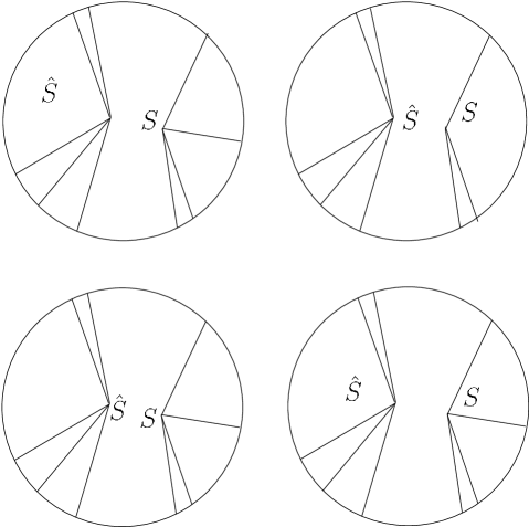
Figure 5. The four possibilities for the relative position of two sectors based at different points

For later reference, let us record several immediate consequences of this picture in the three Lemmas below:

Lemma 4.6.

Let $S$ and $\hat{S}$ be sectors of distinct types of finite cardinality. Then one and only one of the following holds:

(i) $S\cap\hat{S}\neq\emptyset$,

(ii) $S\subset\hat{S}$,

(iii) $\hat{S}\subset S$,

(iv) ${\mathbb{C}}\setminus S\subset\hat{S}$ and ${\mathbb{C}}\setminus\hat{S}\subset S$.

Lemma 4.7.

Let $S$ and $\hat{S}$ be sectors of distinct finite types. Then:

(a) $S\cap\hat{S}\neq\emptyset$ if and only if $\pi_{\infty}S\cap\pi_{\infty}\hat{S}\neq\emptyset$.

(b) $S\subset\hat{S}$ if and only if $\pi_{\infty}S\subset\pi_{\infty}\hat{S}$.

Lemma 4.8.

Consider two distinct finite types $A(z)$ and $A(\hat{z})$ and let $S$ (resp. $\hat{S}$) be a sector with basepoint $z$ (resp. $\hat{z}$) then:

(a) If $S\cap\hat{S}\neq\emptyset$ then $\hat{z}\in S$ or $z\in\hat{S}$.

(b) If $\hat{z}\in S$ then $S$ contains all but one of the sectors based at $\hat{z}$

(c) If $\hat{z}\notin S$ then $S$ is contained in exactly one sector based at $\hat{z}$.

5. Periodic Orbit Portraits

In this section we study types of periodic points which are the landing point of smooth periodic rays. We give an upper bound on the number of cycles of rays that can land at a periodic orbit. The results here are an immediate generalization of the ones obtained by Milnor for quadratic polynomials (see [M2]). In the next Section we will apply similar ideas to give to find an upper bound on the number of external rays landing at a point with infinite forward orbit.

We assign to a periodic orbit portrait a rotation number as follows. Let ${\mathcal{O}}=\{z_{0},f(z_{0}),\dots,f^{\circ(p-1)}(z_{0})\}\subset J(f)$ be a periodic cycle of period $p$ with portrait $A({\mathcal{O}})$ formed by periodic arguments. That is, ${\mathcal{O}}$ is a parabolic or repelling cycle and each point in ${\mathcal{O}}$ is the landing point of smooth periodic rays of the same period. By Lemma 3.4 the return map

$${{m_{d}}^{\circ p}_{|}}_{A(z_{0})}:A(z_{0})\rightarrow A(z_{0})$$

is cyclic order preserving. Thus, the return map has a well defined rotation number $\mbox{rot}A({\mathcal{O}})\in{{\mathbb{Q}}/{\mathbb{Z}}}$ which does not depend on the choice of $z_{0}\in{\mathcal{O}}$. The rotation number of $A({\mathcal{O}})$ is also called the combinatorial rotation number of ${\mathcal{O}}$.

The number of periodic cycles of $A({\mathcal{O}})$ is the number of cycles of $m_{d}$ that participate in $A(z_{0})\cup\cdots\cup A(f^{\circ(p-1)}(z_{0}))$. For a quadratic polynomial, Milnor [M2] showed that the number of cycles of a periodic orbit portrait $A({\mathcal{O}})$ is at most $2$. Moreover, if the number of cycles is $2$ then $A({\mathcal{O}})$ has zero rotation number. We generalize this result:

Theorem 5.1.

The number of cycles of $A({\mathcal{O}})$ is at most $d$. Moreover, if the number of cycles is $d$ then $A({\mathcal{O}})$ has zero rotation number.

The bounds above are obtained by showing that the number of cycles of a portrait gives rise to a lower bound on the number of critical values of the polynomial in question. Hence, we prefer to state the result as follows:

Theorem 5.2.

If $f$ has exactly $k$ distinct critical values then the number of cycles of $A({\mathcal{O}})$ is at most $k+1$. Moreover, if ${A({\mathcal{O}})}$ has $k+1$ cycles then $A({\mathcal{O}})$ has zero rotation number.

Remark: The bounds on the number of cycles are sharp. In fact, every parabolic periodic orbit ${\mathcal{O}}$ with $d-1$ immediate basins and multiplier distinct from $1$ has exactly $d-1$ cycles of rays participating in $A({\mathcal{O}})$. In this case $A({\mathcal{O}})$ has nonzero rotation number (also compare with Figure 3).

Figure 2 shows a cubic periodic orbit portrait with $3$ cycles and zero rotation number.

Notice that the sector map $\tau$ at ${\mathcal{O}}$ is a well defined permutation of the sectors based at ${\mathcal{O}}$. Observe that the number of cycles of sectors under $\tau$ coincides with the number of cycles of external rays participating in $A({\mathcal{O}})$.

The following Lemma (see [M2]) shows that the smallest sector in a cycle contains a critical value:

Lemma 5.3.

If $\alpha(S)=\min\{\alpha(\tau^{\circ n}(S)):n\in{{\mathbb{N}}}\}$ then $v(S)>0$.

Proof: Consider a sector $S$ with minimal angular size in its cycle. If $v(S)=0$ then Lemma 4.5 (c) shows that $w(\tau^{-1}(S))=0$. By Lemma 4.5 (b) we have that $\alpha(\tau^{-1}(S))=\alpha(S)/d$, which contradicts minimality of the angular length. $\Box$

Proof of Theorem 5.2: By contradiction, suppose that $\mbox{rot}{A({\mathcal{O}})}\neq 0$ and that ${A({\mathcal{O}})}$ has more than $k$ cycles. Select $k+1$ sectors $S_{1},\dots,S_{k+1}$ such that:

(a) If $\tau^{\circ n}(S_{i})=S_{j}$ then $i=j$. (i.e. $S_{1},\dots,S_{k+1}$ belong to different cycles of sectors).

(b) The angular length of $S_{i}$ is minimal in its cycle of sectors.

By Lemma 5.3 we have that $v(S_{i})>0$. Thus, in order to obtain a contradiction it is enough to show that $S_{1},\dots,S_{k+1}$ are pairwise disjoint.

If $S_{i}\cap S_{j}\neq\emptyset$ then $S_{i}$ contains the basepoint $z$ of $S_{j}$ or $S_{i}$ contains the basepoint $w$ of $S_{j}$ (Lemma 4.8 (a)). In the first case $S_{i}$ contains all the sectors based at $z$ with the exception of one (Lemma 4.8 (b)). Since the cycle of $S_{i}$ has at least 2 sectors based at $z$ (nonzero rotation number), it follows that $S_{i}$ properly contains a sector in its cycle. This contradicts (b), i.e. minimality of the angular length. The same reasoning gives a contradiction in the second case.

Now suppose that $\mbox{ rot}{A({\mathcal{O}})}=0$ and that ${A({\mathcal{O}})}$ has more than $k+1$ cycles. Consider a minimal angular length sector in each cycle of sectors and select $k+1$ amongst them with smaller angular length. Denote these sectors by $S_{1}\dots S_{k+1}$. Again we obtain a contradiction by showing that they are pairwise disjoint.

If $S_{i}\cap S_{j}\neq\emptyset$ then $S_{i}$ contains the basepoint $z$ of $S_{j}$ or $S_{i}$ contains the basepoint $w$ of $S_{j}$. In the first case, $S_{i}$ contains all the sectors based at $z$ with the exception of one, which has to be in the cycle of $S_{i}$. Hence $S_{i}$ properly contains at least $k+1$ sectors of different cycles, this contradicts the choice of $S_{i}$. The second case is identical. $\Box$

6. Wandering Orbit Portraits

A priori we do not know that the type $A(z)$ of a point $z$ with infinite orbit has finite cardinality. In order to apply the results obtained in Section 4 for types with finitely many elements we restrict our attention to finite subsets of $A(z)$. Accordingly we restrict to finite subsets along the forward orbit of $z$:

Definition 6.1.

Consider an infinite orbit ${\mathcal{O}}$ that does not contain critical values. We say that

$$A^{*}({\mathcal{O}})=\{A^{*}(z):z\in{\mathcal{O}}\}$$

is an orbit sub-portrait of $A({\mathcal{O}})$ if:

$A^{*}(z)\subset A(z)$,

$A^{*}(z)$ is finite and

$m_{d}(A^{*}(z))=A^{*}(f(z))$.

For orbit sub-portraits we can introduce sectors, angular length and the sector map $\tau$ just as we did in Section 4. It is not difficult to check that the results obtained in Section 4 remain valid for sub-portraits.

Observe that if ${\mathcal{O}}=\{z,f(z),\dots\}$ does not contain critical values and $A^{*}(z)$ is a finite subset of $A(z)$ then $\{A^{*}(z),m_{d}(A^{*}(z)),\dots\}$ is an orbit sub-portrait of $A({\mathcal{O}})$.

Remark: In the definition of sub-portraits we avoid orbits containing a critical value for two reasons. The first one is that we exclude the special case in which a critical value does not belong to any of the sectors based at a given point. The second reason is that since an orbit without critical values is also free of critical points we have that the cardinality of $A^{*}(z)$ is independent of $z\in{\mathcal{O}}$.

Proof of Theorem 3.2: Given $z\in J(f)$, as in the statement of the Theorem, pick $N$ such that the forward orbit ${\mathcal{O}}$ of $z_{0}=f^{\circ N}(z)$ does not contain a critical value. First we show that $A(z_{0})$ contains at most $d$ elements.

Consider an orbit sub-portrait ${A^{*}}({\mathcal{O}})$ and assume that the cardinality of $A^{*}(z_{0})$ is $d+1$. After some work we obtain a contradiction.

Let $z_{n}=f^{\circ n}(z_{0})$ and enumerate the sectors of $A^{*}(z_{n})$ based at $z_{n}$ by $S^{1}(n),\dots,S^{d+1}(n)$ according to their angular length:

$$\alpha(S^{1}(n))\leq\alpha(S^{2}(n))\leq\cdots\leq\alpha(S^{d+1}(n)).$$

Intuitively we interpret the angular length of a sector as its size. Under the sector map $\tau$, sectors of angular length beneath $1/d$ increase their size. In contrast, for $n$ large, at most 2 sectors based at $z_{n}$ are not arbitrarily small:

Claim 1: $\lim_{n\rightarrow\infty}\alpha(S^{d-1}(n))=0$.

Proof of Claim 1: By contradiction, suppose that

$$\lim\sup\alpha(S^{d-1}(n))=a>0$$

and let $n_{k}$ be a subsequence such that:

$$\frac{2a}{3}<\alpha(S^{d-1}(n_{k}))<\frac{4a}{3}.$$

The sectors $S^{d-1}(n_{k})$ cannot be disjoint because otherwise we would have infinitely many disjoint intervals of length greater than $2a/3$ contained in ${{\mathbb{R}}/{\mathbb{Z}}}$ (Lemma 4.7). Let $n_{k_{0}}$ and $n_{k_{1}}$ be such that

$$S^{d-1}(n_{k_{0}})\cap S^{d-1}(n_{k_{1}})\neq\emptyset.$$

From Lemma 4.8 (a) we conclude that

$$z_{n_{k_{0}}}\in S^{d-1}(n_{k_{1}})\mbox{ or }z_{n_{k_{1}}}\in S^{d-1}(n_{k_{0}}).$$

Without loss of generality, $z_{n_{k_{0}}}\in S^{d-1}(n_{k_{1}})$. This implies that all the sectors based at $z_{n_{k_{0}}}$ with the exception of one are contained in $S^{d-1}(n_{k_{1}})$. Since there are 3 sectors

$$S^{d-1}(n_{k_{0}}),S^{d}(n_{k_{0}}),S^{d+1}(n_{k_{0}})$$

based at $z_{n_{k_{0}}}$ of angular length greater than $2a/3$ it follows that at least 2 of these must be contained in $S^{d-1}(n_{k_{1}})$. Thus, the angular length of $S^{d-1}(n_{k_{1}})$ is greater than $4a/3$ which is impossible.

For our purposes we do not distinguish between critical values that lie in the same sector based at $z_{n}$ for all $n$. That is, critical values $v$ and $v^{\prime}$ such that $v\in S^{k}(n)$ if and only if $v^{\prime}\in S^{k}(n)$ are regarded as ONE critical value of $f$. With this in mind, for each critical value $v$ let

$$\delta(v)=\inf\{\alpha(S^{k}(n)):v\in S^{k}(n)\}.$$

Observe that $\delta(v)=0$ if and only if $v$ is contained in an arbitrarily small sector.

Loosely speaking, we want to show that there is a correspondence between sectors that become arbitrarily small and critical values $v$ such that $\delta(v)=0$. In order to establish this correspondence we need to “isolate” each critical value $v$ such that $\delta(v)=0$ from the rest of the critical values of $f$.

Let

$$\epsilon=\min\{\delta(v):\delta(v)\neq 0\}\cup\{1/d\}.$$

Claim 2: For each critical value $v$ such that $\delta(v)=0$ there exists $n(v)$ such that:

(a) The sector $S(n(v))$ based at $z_{n(v)}$ containing $v$ has angular length $\alpha(S(n(v)))<\epsilon$.

(b) $v^{\prime}\notin S(n(v))$ for all critical values $v^{\prime}\neq v$.

(c) $S(n(v))\cap S(n(v^{\prime}))=\emptyset$ for all critical values $\delta(v^{\prime})=0$.

Proof of Claim 2: For parts (a) and (b) enumerate by $v_{1}\dots v_{m}$ the critical values of $f$ distinct from $v$. We already identified the critical values that always belong to the same sector so there exists sectors $S_{v_{1}},\dots,S_{v_{m}}$ such that $v\in S_{v_{k}}$ and $v_{k}\notin S_{v_{k}}$. Now the critical value $v$ is contained in arbitrarily small sectors ($\delta(v)=0$), thus there exists an integer $n(v)$ such that the sector $S(n(v))$ based at $z_{n(v)}$ containing $v$ has angular length:

$$\alpha(S(n(v)))<\min\{\alpha(S_{v_{k}}),1-\alpha(S_{v_{k}}):k=1,\dots,m\}\cup\{\epsilon\}.$$

The sectors $S(n(v))$ and $S_{v_{k}}$ are not disjoint because both contain $v$. By Lemma 4.6 we know that one of the following holds:

$$S(n(v))\subset S_{v_{k}},$$

$$S_{v_{k}}\subset S(n(v)),$$

$${\mathbb{C}}\setminus S_{v_{k}}\subset S(n(v)).$$

The upper bound on $\alpha(S(n(v)))$ says that only the first possibility can hold. It follows that $v_{k}\notin S(n(v))$ for all $k$.

For part (c), if $S(n(v))\cap S(n(v^{\prime}))\neq\emptyset$ then one of the following holds

$$S(n(v))\subset S(n(v^{\prime}))$$

$$S(n(v^{\prime}))\subset S(n(v))$$

$${\mathbb{C}}\setminus S(n(v^{\prime}))\subset S(n(v))$$

Part (b) of this Claim rules out the first and second possibility. The third one implies that

$$\alpha(S(n(v)))>1-\alpha(S(n(v^{\prime})))\geq 1-\epsilon\geq\epsilon,$$

which contradicts part (a) and finishes the proof of Claim 2.

In the next claim we start to establish the correspondence between small sectors and critical values:

Claim 3: There exists $N_{0}$ such that $S^{1}(N_{0})$ contains a critical value and

(a) $\alpha(S^{1}(N_{0}))\leq\alpha(S^{1}(n(v)))$ for all critical values $v$ such that $\delta(v)=0$.

(b) $\alpha(S^{1}(N_{0}))<\epsilon$.

Proof of Claim 3: From Claim 1 we know that there exists $M$ such that for all $n\geq M$:

$\alpha(S^{1}(n))\leq\alpha(S(n(v)))$ for all $v$ such that $\delta(v)=0$ and,

$\alpha(S^{1}(n))<\epsilon$.

Now, for some $N_{0}\geq M$, the sector $S^{1}(N_{0})$ must contain a critical value, otherwise $\alpha(S^{1}(n))$ would be increasing for $n\geq M$.

We think of $\alpha(S^{1}(N_{0}))$ as the threshold for a sector to be considered “big” or “small”. That is, if a sector has angular length greater (resp. less) than $\alpha(S^{1}(N_{0}))$ is thought as being “big” (resp. “small”). Now we show that in the transition from sectors based at $z_{n}$ to the sectors based at $z_{n+1}$ at most one sector that is “big” can “become small”.

Claim 4: If $\alpha(S^{j}(n))\geq\alpha(S^{1}(N_{0}))$ then $\alpha(\tau(S^{j+1}(n+1)))\geq\alpha(S^{1}(N_{0}))$.

Proof of Claim 4: By contradiction, if $\alpha(\tau(S^{j+1}(n+1)))<\alpha(S^{1}(N_{0}))$ then there are at least 2 sectors $S$ and $S^{\prime}$ based at $z_{n}$ such that:

$$\alpha(S)\geq\alpha(S^{1}(N_{0}))>\alpha(\tau(S))\mbox{ and}$$

$$\alpha(S^{\prime})\geq\alpha(S^{1}(N_{0}))>\alpha(\tau(S^{\prime}))$$

Hence, $\tau(S)$ (resp. $\tau(S^{\prime})$) contains a critical value $v$ (resp. $v^{\prime}$). Since $\alpha(\tau(S))<\alpha(S^{1}(N_{0}))\leq\alpha(S(n(v)))$ it follows that $\tau(S)\subset S(n(v))$. Similarly $\tau(S^{\prime})\subset S(n(v^{\prime}))$. This implies that the common basepoint $z_{n+1}$ of the sectors $\tau(S)$ and $\tau(S^{\prime})$ is contained both in $S(n(v))$ and in $S(n(v^{\prime}))$ which contradicts Claim 2 part (c).

For $1\leq k\leq d-1$, let $N_{k}$ be the smallest integer greater than $N_{0}$ such that $\alpha(S^{k}(N_{k}))<\alpha(S^{1}(N_{0}))$. That is, $z_{N_{k}}$ is the first iterate after $z_{N_{0}}$ for which $k$ of the sectors based at $z_{N_{k}}$ are “small”. Observe that $N_{0}\leq N_{1}\leq\dots\leq N_{d-1}$ and that the existence of such integers $N_{k}$ is guaranteed by Claim 1. We need to show that there are at least two “big” sectors based at each $z_{N_{k}}$:

Claim 5: $S^{d}(N_{k})\geq S^{1}(N_{0})$ for $0\leq k\leq d-1$.

Proof of Claim 5: For $k=0$ the claim is trivial. Given $k\geq 1$ we have that $\alpha(S^{k}(N_{k}-1))\geq\alpha(S^{1}(N_{0}))$ and by the previous Claim we conclude that $\alpha(S^{k+1}(N_{k}))\geq\alpha(S^{1}(N_{0}))$. Since $\alpha(S^{d}(N_{k}))\geq\alpha(S^{k+1}(N_{k}))$ we are done.

For $1\leq k\leq d-1$, let $l_{k}$ be such that

$$\alpha(S^{l_{k}}(N_{k}-1))\geq\alpha(S^{1}(N_{0}))>\alpha(\tau(S^{l_{k}}(N_{k}-1))).$$

Claim 6: $S^{1}(N_{0}),\tau(S^{l_{1}}(N_{1}-1)),\dots\tau(S^{l_{d-1}}(N_{d-1}-1))$ are disjoint and each contains a critical value.

Proof of Claim 6: By Claim 4 and Lemma 4.5 (d), we know that these sectors contain critical values. Now we have to show that they are disjoint. If $\tau(S^{l_{k_{0}}}(N_{k_{0}}-1))\cap\tau(S^{l_{k_{1}}}(N_{k_{1}}-1))\neq\emptyset$ then without loss of generality we may assume that $z_{N_{k_{0}}}\in\tau(S^{l_{k_{1}}}(N_{k_{1}}-1))$. Lemma 4.8 (b) implies that all but one of the sectors based at $z_{N_{k_{0}}}$ are contained in $\tau(S^{l_{k_{1}}}(N_{k_{1}}-1))$. From Claim 5, there is at least one sector of angular length greater then $\alpha(S^{1}(N_{1}))$ contained in $\tau(S^{l_{k_{1}}}(N_{k_{1}}-1))$. That is,

$$\alpha(\tau(S^{l_{k}}(N_{k}-1)))\geq\alpha(S^{1}(N_{0}))$$

which is a contradiction. This finishes the proof of Claim 6.

Remark: If a critical value $v$ is contained in one of the sectors   $S^{1}(N_{0})$, $\tau(S^{l_{1}}(N_{1}-1)),\ \dots\ \tau(S^{l_{d-1}}(N_{d-1}-1))$ then $\delta(v)=0$ (the angular length of each of these sectors is less than $\epsilon$).

It follows from Claim 6 and the fact that polynomials of degree $d$ have at most $d-1$ critical values that the cardinality of $A(f^{\circ N}(z))$ is at most $d$.

We modify the arguments above in order to show that the cardinality of $A(z)$ is at most $2^{d}$.

Let $b$ be the number of critical values that are not in the forward orbit of $z$. First suppose that $b\geq 1$, and replace $d$ by $b+1$ in all the statements from the beginning of the proof up to the end of Claim 6. That is, suppose that there are $b+2$ rays landing at $f^{\circ N}(z)$ and obtain $b+1$ critical values $v$ such that $\delta(v)=0$. This is a contradiction because all the critical values in the forward orbit of $z$ cannot be contained in arbitrarily small sectors, hence there are at most $b$ critical values $v$ with $\delta(v)=0$. Now that we know that at most $b+1$ rays land at $f^{\circ N}(z)$ let $m_{1},\dots,m_{a}$ be the multiplicity of the critical points in forward orbit of $z$. Hence, $A(z)$ has cardinality at most

$$(m_{1}+1)\cdots(m_{a}+1)\cdot(b+1).$$

Since the sum $(m_{1}+1)+\cdots+(m_{a}+1)\leq d-1-b+a$ and $m_{k}+1\geq 2$, it is not difficult to show that $(m_{1}+1)\cdots(m_{a}+1)\leq 2^{d-1-b}$. Then

$$(m_{1}+1)\cdots(m_{a}+1)\cdot(b+1)\leq 2^{d-1-b}(b+1)\leq 2^{d}.$$

Now suppose that $b=0$ and replace $d$ by $2$, starting at the beginning of the proof up to the end of Claim 3. That is, assume that $3$ rays land at $f^{\circ N}(z)$ and obtain a critical value $v$ such that $\delta(v)=0$, this is impossible because all the critical values are in the orbit of $z$. Hence, the cardinality of $A(f^{\circ N}(z))$ is at most 2. The product of the local degree of $f$ at the critical points is at most $2^{d-1}$. Therefore, when $b=0$ we also have that $A(z)$ contains at most $2^{d}$ elements. $\Box$

Chapter 2: The Shift Locus

7. Introduction

In parameter space, following Branner and Hubbard [BH], we work in the set ${{\mathcal{P}}_{d}}\cong{\mathbb{C}}^{d-1}$ of monic centered polynomials of degree $d$. Namely, polynomials of the form:

$$z^{d}+a_{d-2}z^{d-2}+\cdots+a_{0}.$$

Parameter space ${{\mathcal{P}}_{d}}$ is stratified according to how many critical points escape to $\infty$. One extreme is the connectedness locus ${{\mathcal{C}}_{d}}\subset{{\mathcal{P}}_{d}}$, which is the set of polynomials $f$ that have connected Julia set $J(f)$. Equivalently, all the critical points of $f$ are non-escaping. The other extreme is the shift locus ${{\mathcal{S}}_{d}}\subset{{\mathcal{P}}_{d}}$, formed by the polynomials $f$ that have all their critical points escaping. In this Chapter we prepare ourselves to explore the set $\partial{{\mathcal{S}}_{d}}\cap{{\mathcal{C}}_{d}}$ where these two extremes meet.

The connectedness locus ${{\mathcal{C}}_{d}}$ is compact, connected and cellular (see [DH0, BH, La]). For $d\geq 3$, ${{\mathcal{C}}_{d}}$ is known not to be locally connected [La]. In contrast, the quadratic connectedness locus, better known as the Mandelbrot set $\mathcal{M}$, is conjectured to be locally connected (see [DH1]).

The dynamics of a polynomial $f$ in the shift locus ${{\mathcal{S}}_{d}}$ is completely understood. In fact, $f$ has a Cantor set as Julia set $J(f)$ and, $f$ acts on $J(f)$ as a hyperbolic dynamical system which is topologically conjugate to the one sided shift in $d$ symbols. The shift locus ${{\mathcal{S}}_{d}}$ is open, connected and unbounded. For $d\geq 3$, ${{\mathcal{S}}_{d}}$ has a highly non-trivial topology. More precisely, its fundamental group is infinitely generated [BDK]. In contrast, after Douady and Hubbard [DH0], the quadratic shift locus $\mathcal{S}_{2}={\mathbb{C}}\setminus\mathcal{M}$ is conformally isomorphic to the complement ${{\mathbb{C}}\setminus\overline{{\mathbb{D}}}}$ of the unit disk.

In the dynamical plane, we describe the location of points in the Julia set, which is the boundary of the basin of infinity, by means of external rays and prime end impressions. In parameter space, we introduce objects that will allow us to explore the portion of $\partial{{\mathcal{S}}_{d}}$ contained in ${{\mathcal{C}}_{d}}$. More precisely, we define what it means to go from the shift locus ${{\mathcal{S}}_{d}}$ towards the connectedness locus ${{\mathcal{C}}_{d}}$ in a given direction. Each direction will be specified by a “critical portrait” and will determine an “impression” in the connectedness locus ${{\mathcal{C}}_{d}}$.

In Chapter 4, we are going to show that the “combinatorics” of a polynomial $f$ in $\partial{{\mathcal{S}}_{d}}\cap{{\mathcal{C}}_{d}}$ is completely determined by the “impression(s)” to which $f$ belongs, provided that $f$ has all its cycles repelling.

For quadratic polynomials, we have a dynamically defined conformal isomorphism from $\mathcal{S}_{2}={\mathbb{C}}\setminus\mathcal{M}$ onto ${{\mathbb{C}}\setminus\overline{{\mathbb{D}}}}$ (see [DH0, DH1]). This map provides us with parameter rays and a dynamical parameterization of the prime end impressions of $\mathcal{S}_{2}$ in $\partial\mathcal{M}$. For higher degrees, we need to overcome the difficulties that stem from the non-trivial topology of the shift locus. Motivated by Goldberg [G], it is better to work with a dense subset of ${{\mathcal{S}}_{d}}$ where the critical points are easily located by the Böttcher coordinates. That is, the polynomials $f$ such that each critical point of $f$ is “visible” from $\infty$, in the sense defined below. Recall that an external radius is a gradient $\mathrm{grad}g_{f}$ flow line that reaches $\infty$ (see 2).

Definition 7.1 (Visible Shift Locus).

Consider a polynomial $f$ which belongs to the shift locus ${{\mathcal{S}}_{d}}$. We say that $f$ belongs to the visible shift locus ${{\mathcal{S}}^{vis}_{d}}$ if for each critical point $c$ of $f$:

(a) there are exactly $k$ external radii terminating at $c$, where $k$ is the local degree of $f$ at $c$;

(b) the critical value $f(c)$ belongs to an external radius.

Our definition has a slight difference with Goldberg’s definition of the “generic shift locus”. Thus, although we use a different name, there is a strong overlap with the ideas found in [G].

The quadratic shift locus coincides with the quadratic visible shift locus. In fact, for a quadratic polynomial $f(z)=z^{2}+a_{0}$ in the shift locus $\mathcal{S}_{2}={\mathbb{C}}\setminus\mathcal{M}$ there are two external radii $R^{*\theta}_{f}$ and $R^{*\theta+1/2}_{f}$ which terminate at the unique critical point $c=0$. Both of these external radii map into $R^{*2\theta}_{f}$ which contains the critical value $f(c)=a_{0}$. Similarly, a polynomial, of any degree, with a unique escaping critical point always lies in the visible shift locus (see Corollary 8.2).

For a cubic polynomial $f\in\mathcal{S}_{3}$ with two distinct critical points, there are three cases. Namely, two external radii might terminate at each critical point, or two external radii terminate at one and four at the other, or two external radii terminate at one and none at the other (see Figure 6). The first case is the only one allowed in the visible shift locus $\mathcal{S}_{3}$, here, external radii with arguments $\{\theta_{1},\theta_{1}+1/3\}$ terminate at one critical point and external radii with arguments $\{\theta_{2},\theta_{2}+1/3\}$ terminate at the other. In the second case, one critical point eventually maps to the other. In the third case, one critical point lies on external rays that bounce off some iterated pre-image of the other critical point.

Figure 6. The possible configurations of gradient flow lines connecting the critical point(s) of a cubic polynomial to $\infty$. Only the upper two are allowed in the visible shift locus $\mathcal{S}^{vis}_{3}$

We keep track of the external radii that terminate at the critical points:

Definition 7.2.

Let $f$ be a polynomial in the visible shift locus ${{\mathcal{S}}^{vis}_{d}}$ with critical points $c_{1},\dots,c_{m}$ and $\Theta_{i}\subset{{\mathbb{R}}/{\mathbb{Z}}}$ be the set formed by the arguments of the external radii that terminate at $c_{i}$. We say that $\Theta(f)=\{\Theta_{1},\dots,\Theta_{m}\}$ is the critical portrait of $f$.

The main properties of ${\Theta}(f)$ are (see Lemma 8.3):

(CP1) For every $j$, $|\Theta_{j}|\geq 2$ and $|m_{d}(\Theta_{j})|=1$,

(CP2) $\Theta_{1},\dots,\Theta_{m}$ are pairwise unlinked,

(CP3) $\sum(|\Theta_{j}|-1)=d-1$.

Definition 7.3 (Critical Portraits).

A collection $\Theta=\{\Theta_{1},\dots,\Theta_{m}\}$ of finite subsets of ${{\mathbb{R}}/{\mathbb{Z}}}$ is called a critical portrait of degree $d$ if (CP1), (CP2) and (CP3) hold.

Critical portraits were introduced by Fisher [F] to study critically pre-repelling maps and, since then, widely used in the literature to capture the location of the critical points (e.g. [BL, P, GM, G]).

A result, due to Goldberg [G], says that for each critical portrait ${\Theta}$ there exists a map $f\in{{\mathcal{S}}^{vis}_{d}}$ such that ${\Theta}(f)={\Theta}$.

For $f\in{{\mathcal{S}}^{vis}_{d}}$, the external radii which terminate at the critical points cut the plane into $d$ components. In order to capture this situation in the circle at infinity, we define ${\Theta}$-unlinked classes.

Definition 7.4.

We say that $t,t^{\prime}\in{{\mathbb{R}}/{\mathbb{Z}}}$ are ${\Theta}=\{{\Theta}_{1},\dots,{\Theta}_{m}\}$-unlinked equivalent if $\{t,t^{\prime}\},{\Theta}_{1},\dots,{\Theta}_{m}$ are pairwise unlinked.

Given a degree $d$ critical portrait $\Theta$, there are exactly $d$ $\Theta$-unlinked classes $L_{1},\dots,L_{d}$. Moreover, each unlinked class $L_{j}$ is the union of open intervals with total length $1/d$. Intuitively, for polynomials in ${{\mathcal{S}}^{vis}_{d}}$ close to $f$, this partition does not change to much. Formally, we introduce a topology on the set of all critical portraits:

Definition 7.5.

Let ${\mathcal{A}}_{d}$ be the set formed by all critical portraits endowed with the compact-unlinked topology which is generated by the subbasis formed by

$$V_{X}=\{\Theta\in{\mathcal{A}}_{d}:X\subset L_{\Theta}\}$$

where $X$ is a closed subset of ${{\mathbb{R}}/{\mathbb{Z}}}$ and $L_{{\Theta}}$ is a ${\Theta}$-unlinked class.

Remark: For “low” degrees, a critical portrait ${\Theta}$ is uniquely determined by the set ${\Theta}^{\cup}$ of angles which participate in ${\Theta}$ and the compact-unlinked topology in ${\mathcal{A}}_{d}$ coincides with the Hausdorff topology on subsets ${\Theta}^{\cup}$ of ${{\mathbb{R}}/{\mathbb{Z}}}$. For “high” degrees, this is not true. In fact, consider the degree six critical portraits

$$\{\{1/12,1/4,7/12,3/4\},\{1/3,1/2\},\{5/6,0\}\},$$

$$\{\{1/12,1/4\},\{7/12,3/4\},\{1/3,1/2,5/6,0\}\}.$$

The set of quadratic critical portraits $\mathcal{A}_{2}$ is homeomorphic to ${{\mathbb{R}}/{\mathbb{Z}}}$. The homeomorphism is given by $\{\theta,\theta+1/2\}\mapsto 2\theta$. The set of cubic critical portraits $\mathcal{A}_{3}$ can be obtained from a Möbius band $M$ as follows. Parameterize the boundary of $M$ by ${{\mathbb{R}}/{\mathbb{Z}}}$ and identify $\beta,\beta+1/3$ and $\beta+2/3$. The resulting topological space is homeomorphic to $\mathcal{A}_{3}$. In general, for $d\geq 3$, ${\mathcal{A}}_{d}$ is compact and connected but it is not a manifold (Lemma 10.1). The set of critical portraits ${\mathcal{A}}_{d}$ is homeomorphic to the subset $\mathcal{E}\subset{{\mathcal{S}}_{d}}$ of polynomials $f$ such that all the critical points $c$ of $f$ escape to $\infty$ at a fixed rate $\rho=g_{f}(c)$ (see Lemma 10.1). The topology of $\mathcal{E}$, for cubic polynomials, has been previously described by Branner and Hubbard in [BH].

Now, the topology in the set of critical portraits allows us to introduce the impression of a critical portrait ${\Theta}$ in the connectedness locus ${{\mathcal{C}}_{d}}$:

Definition 7.6.

Let ${\Theta}$ be a critical portrait. We say that $f$ belongs to the impression $I_{{{\mathcal{C}}_{d}}}({\Theta})$ of the critical portrait ${\Theta}$ if there exists a sequence of maps $f_{n}\in{{\mathcal{S}}^{vis}_{d}}$ converging to $f$ such that the corresponding critical portraits ${\Theta}(f_{n})$ converge to ${\Theta}$.

For quadratic polynomials, $I_{\mathcal{M}}(\{\theta,\theta+1/2\})$ is a prime end impression. More precisely, it is the prime end impression corresponding to $2\theta$ under the Douady-Hubbard map $\Phi:{\mathbb{C}}\setminus\mathcal{M}\rightarrow{{\mathbb{C}}\setminus\overline{{\mathbb{D}}}}$.

In order to show that impressions of critical portraits are connected and cover all of $\partial{{\mathcal{S}}_{d}}\cap{{\mathcal{C}}_{d}}$ we study the basic properties of the map $\Pi$ from ${{\mathcal{S}}^{vis}_{d}}$ onto the set of critical portraits ${\mathcal{A}}_{d}$. The following Theorem asserts that critical portraits depend continuously on $f\in{{\mathcal{S}}^{vis}_{d}}$. Also, the set $S_{{\Theta}}$ of polynomials in ${{\mathcal{S}}^{vis}_{d}}$ which share a common critical portrait ${\Theta}$ form a sub-manifold of ${{\mathcal{S}}_{d}}$ parameterized by the escape rates of the critical points:

Theorem 7.7.

The subset ${{\mathcal{S}}^{vis}_{d}}$ is dense in ${{\mathcal{S}}_{d}}$, and the map

$$\begin{array}[]{lccl}{\Pi}:&{{\mathcal{S}}^{vis}_{d}}&\rightarrow&{\mathcal{A}}_{d}\\ &f&\mapsto&\Theta(f)\\ \end{array}$$

is continuous and onto.

Moreover, for any critical portrait ${\Theta}=\{{\Theta}_{1},\dots,{\Theta}_{m}\}$, the preimage $S_{\Theta}=\mathbf{\Pi}^{-1}({\Theta})$ is a $m$-real dimensional manifold. In fact, let

$$\begin{array}[]{lccl}G:&S_{{\Theta}}&\rightarrow&{\mathbb{R}}^{m}_{>0}\\ &f&\mapsto&(g_{f}(c_{1}),\dots,g_{f}(c_{m}))\\ \end{array}$$

where $c_{i}$ is the critical point corresponding to $\Theta_{i}$. Then $G$ is injective and

$$G(S_{\Theta})=\{(r_{1},\dots,r_{m}):d^{n}\cdot{\Theta}_{i}\in{\Theta}_{j}\Rightarrow d^{n}r_{i}>r_{j}\}.$$

The proof of this Theorem appears in Section 9. Afterwards, in Section 10, we deduce the following:

Corollary 7.8.

The impression $I_{{{\mathcal{C}}_{d}}}({\Theta})$ of a critical portrait ${\Theta}$ is a non empty and connected subset of $\partial{{\mathcal{S}}_{d}}\cap{{\mathcal{C}}_{d}}$. Moreover,

$$\bigcup_{{\Theta}\in{\mathcal{A}}_{d}}I_{{{\mathcal{C}}_{d}}}({\Theta})=\partial{{\mathcal{S}}_{d}}\cap{{\mathcal{C}}_{d}}.$$

Remark: For quadratic polynomials, the sub-manifolds $S_{{\Theta}}$ are the parameter rays introduced by Douady and Hubbard in [DH1]. For cubic polynomial, if ${\Theta}=\{{\Theta}_{1},{\Theta}_{2}\}$ then $S_{{\Theta}}$ is an interval worth of Branner-Hubbard “stretching” rays (see [BH]). If ${\Theta}=\{\theta,\theta+1/3,\theta+2/3\}$ then $S_{{\Theta}}$ is a parameter ray in the parameter plane of the family $z^{3}+a_{0}$.

8. Dynamical Plane

For $f$ in the shift locus ${{\mathcal{S}}_{d}}$, the Julia set $J(f)$ is a measure zero Cantor set and, on $J(f)$, the map $f$ is topologically conjugate to the one sided shift on $d$ symbols (see [Bl]).

In Section 2, we summarized some results about polynomials with disconnected Julia set. Here, we go into more details about polynomials in the visible shift locus ${{\mathcal{S}}^{vis}_{d}}$.

In the introduction, we defined ${{\mathcal{S}}^{vis}_{d}}$ by imposing conditions on the external radii that terminate at critical points. Sometimes it is easier to look at the gradient flow nearby the critical points. Recall that at the critical points $\mathrm{grad}g_{f}$ vanishes and that the reduced basin of infinity $\Omega^{*}(f)$ is the basin of infinity under the gradient flow (Section 2).

Lemma 8.1.

A polynomial $f\in{{\mathcal{S}}_{d}}$ lies in ${{\mathcal{S}}^{vis}_{d}}$ if and only if for each critical point $c$ of $f$:

(a) there are exactly $k$ local unstable manifolds of the gradient flow at $c$, where $k$ is the local degree of $f$ at $c$,

(b) each local unstable manifold of $\mathrm{grad}g_{f}$ at $c$ is contained in $\Omega^{*}(f)$.

Proof: It is not difficult to show that if $f\in{{\mathcal{S}}^{vis}_{d}}$ then conditions (a) and (b) hold. Conversely, (b) implies that each of the local unstable manifold of $c$ must lie in an external radius which terminates at $c$. These $k$ external radii must map, under $f$, into the same external radius $R^{*t}_{f}$. Hence, either $R^{*t}_{f}$ terminates at $f(c)$ or $R^{*t}_{f}$ contains $f(c)$. In the first case we have that $f(c)$ must be a pre-critical point. Thus, the number of unstable manifolds around $c$ would be greater then $k$, which contradicts (a). Therefore, $R^{*t}_{f}$ contains $f(c)$ and $f\in{{\mathcal{S}}^{vis}_{d}}$. $\Box$

As an immediate consequence we have that:

Corollary 8.2.

If $f\in{{\mathcal{S}}_{d}}$ is such that all the critical points $c$ of $f$ have the same escape rate $\rho=g_{f}(c)$ then $f$ lies in the visible shift locus ${{\mathcal{S}}^{vis}_{d}}$.

In particular, any polynomial of the form $z\mapsto z^{d}+a_{0}$ which belongs to ${{\mathcal{S}}_{d}}$ also belongs to ${{\mathcal{S}}^{vis}_{d}}$.

For the rest of this section, unless otherwise stated, $f$ is a polynomial in the visible shift locus ${{\mathcal{S}}^{vis}_{d}}$. The basic properties of the critical portrait of $f$ are stated below:

Lemma 8.3.

Let $f$ be a polynomial in the visible shift locus ${{\mathcal{S}}^{vis}_{d}}$ with critical points $c_{1},\dots,c_{m}$ and critical portrait $\Theta(f)=\{\Theta_{1},\dots,\Theta_{m}\}$, where $\Theta_{i}$ is formed by the arguments of the external radii that terminate at $c_{i}$. Then

(CP1) For every $j$, $|\Theta_{j}|\geq 2$ and $|m_{d}(\Theta_{j})|=1$,

(CP2) $\Theta_{1},\dots,\Theta_{m}$ are pairwise unlinked,

(CP3) $\sum(|\Theta_{j}|-1)=d-1$.

Proof: For (CP1), observe that the external radii that terminate at $c_{i}$ must map into the unique external radius or ray which contains the critical value $f(c_{i})$. For (CP2), just notice that external radii are disjoint. By counting multiplicities (CP3) follows. $\Box$

From the critical portrait ${\Theta}(f)$ and the escape rates of the critical points of $f$ we can describe the image $U_{f}$ of the Böttcher map:

$$\phi_{f}:\Omega^{*}(f)\rightarrow U_{f}.$$

In fact, assume that ${\Theta}(f)=\{{\Theta}_{1},\dots,{\Theta}_{m}\}$ is the critical portrait of $f$ and $g_{f}(c_{1}),\dots,g_{f}(c_{m})$ are the escape rates of the corresponding critical points. Following Levin and Sodin [LS], for each $\theta\in{\Theta}_{i}$, let $I_{\theta}\subset{\mathbb{C}}\setminus{\mathbb{D}}$ be the “needle” based at $e^{2\pi i\theta}$ of height $e^{g_{f}(c_{i})}$:

$$I_{\theta}=[1,e^{g_{f}(c_{i})}]e^{2\pi i\theta}.$$

Now consider all the iterated preimages of

$$\bigcup_{\theta\in{\Theta}_{1}\cup\dots\cup{\Theta}_{m}}I_{\theta}$$

under the map $z\mapsto z^{d}$ to obtain a “comb” $C\subset{\mathbb{C}}\setminus{\mathbb{D}}$. It follows that the “hedgehog” $\overline{{\mathbb{D}}}\cup C$ is the complement of $U_{f}$. Equivalently, $U_{f}={\mathbb{C}}\setminus\overline{{\mathbb{D}}}\cup C$ (see Figure 7).

Example 1: Consider a quadratic polynomial $f_{v}:z\mapsto z^{2}+v$ where $v$ is real and $v>1/4$. The external radii with arguments $0$ and $1/2$ terminate at the critical point $0$ and ${\Theta}(f_{v})=\{0,1/2\}$. Say that the escape rate of $0$ is $\log r$. Then the “hedgehog” for $f_{v}$ is the closed unit disk $\overline{{\mathbb{D}}}$ union a comb of needles based at every point of the form $e^{2\pi ip/2^{n}}$. For $p$ odd, at each point $p/2^{n}$ the needle has height $r^{1/2^{n-1}}$ and at $1\in\partial{\mathbb{D}}$ the needle has height $r$.

Figure 7. Hedgehog

A point $e^{\rho+2\pi it}$ belongs to $U_{f}$ if either $d^{n}t\notin{\Theta}_{1}\cup\dots\cup{\Theta}_{m}$, or $d^{n}t\in{\Theta}_{i}$ and $d^{n}\rho>g_{f}(c_{i})$. Since each critical value $f(c_{i})$ belongs to $\Omega^{*}(f)$ and $\phi_{f}(f(c_{i}))=e^{g_{f}(c_{i})+2\pi id{\Theta}_{i}}$ we have that:

$$d^{n}\cdot{\Theta}_{i}\in{\Theta}_{j}\Rightarrow d^{n}g_{f}(c_{i})>g_{f}(c_{j}).$$

This explains why in the statement of Theorem 7.7 the image of $G$ is contained in

$$\{(r_{1},\dots,r_{m}):d^{n}\cdot{\Theta}_{i}\in{\Theta}_{j}\Rightarrow d^{n}r_{i}>r_{j}\}.$$

Lemma 8.4.

In the notation of Theorem 7.7,

$$G(S_{\Theta})\subset\{(r_{1},\dots,r_{m}):d^{n}\cdot{\Theta}_{i}\in{\Theta}_{j}\Rightarrow d^{n}r_{i}>r_{j}\}.$$

Also note that for

$$t\notin\Sigma=\bigcup_{n\geq 0}m_{d}^{-n}({\Theta}_{1}\cup\dots\cup{\Theta}_{m})$$

the external ray $R^{t}_{f}$ is smooth. For $t\in\Sigma$ we have two non-smooth external rays $R^{t^{+}}_{f}$ and $R^{t^{-}}_{f}$ which bounce off some pre-critical point(s).

Example 1: (continued) For a quadratic polynomial $f_{v}:z\mapsto z^{2}+v$ where $v>1/4$, the external rays with arguments of the form $p/2^{n}$ eventually map to one of the fixed non-smooth external rays $R^{0^{\pm}}_{f_{v}}$ which contain the critical point. It follows that the external rays with argument $p/2^{n}$ are not smooth.

Example 2: Consider a cubic polynomial $f\in\mathcal{S}^{vis}_{3}$ with critical portrait $\{{\Theta}_{1}=\{1/3,2/3\},{\Theta}_{2}=\{1/9,7/9\}\}$. Then $g_{f}(c_{2})>g_{f}(c_{1})/3$. The external rays with arguments of the form $p/3^{q}$, where $p\neq 0$, are not smooth because $m^{\circ q-1}_{3}(p/3^{q})=1/3\mbox{ or }2/3$.

The external radii with arguments in ${\Theta}_{1}\cup\dots\cup{\Theta}_{m}$ together with the critical points chop the complex plane into $d$ connected components $U_{1},\dots,U_{d}$. The boundary of $U_{i}$ is formed by pairs of external radii that terminate at a common critical point. Each of these pairs is mapped onto an arc which joins a critical value to $\infty$. Moreover, $f$ maps $U_{i}$ homeomorphically onto a slited complex plane and $\overline{U}_{i}$ onto ${\mathbb{C}}$ (see Figure 8).

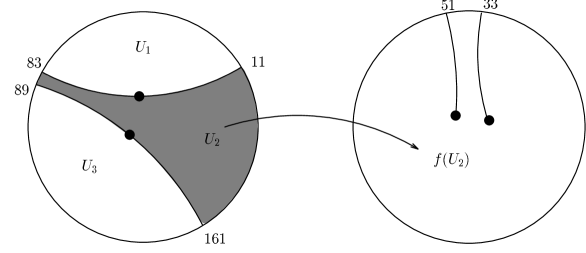
Figure 8. Schematic picture of the external radii terminating at the critical points of a cubic polynomial $f$ with critical portrait $\{\{11/216,83/216\},\{89/216,161/216\}\}$. Also we illustrate the image of these external radii and of the region $U_{2}$. Units are in $1/216$.

In the circle at infinity, each connected component $U_{i}$ spans a $\Theta$-unlinked class $L_{i}$. Each ${\Theta}$-unlinked class $L_{i}$ is a finite union of intervals with total length $1/d$. The boundary points of $L_{i}$ are mapped two to one by $m_{d}$ and $L_{i}$ is mapped injectively onto its image.

Example 3: Consider a cubic polynomial $f$ with critical portrait

$${\Theta}=\{\{11/216,83/216\},\{89/216,161/216\}\}.$$

The ${\Theta}$-unlinked classes are $L_{1}=(11/216,83/216)$,

$$L_{2}=(83/216,89/216)\cup(161/216,11/216)$$

and $L_{3}=(89/216,161/216)$. The schematic situation is represented in Figure 8.

Since the Julia set $J(f)$ is a Cantor set, every external ray lands. The symbolic dynamics induced on $J(f)$ by the connected components $U_{1},\dots,U_{d}$ corresponds to the symbolic dynamics induced on the arguments of the external rays by the ${\Theta}(f)$-unlinked classes.

Definition 8.5.

Given a critical portrait ${\Theta}$ of degree $d$ with ${\Theta}$-unlinked classes $L_{1},\dots,L_{d}$, let

$$\begin{array}[]{lccl}\mathrm{itin}^{\pm}_{\Theta}:&{{\mathbb{R}}/{\mathbb{Z}}}&\rightarrow&\{1,\dots,d\}^{{{\mathbb{N}}}\cup\{0\}}\\ &t&\mapsto&(j_{0},j_{1},\dots)\\ \end{array}$$

if, for each $n\geq 0$, there exists $\epsilon>0$ such that $(d^{n}t,d^{n}t\pm\epsilon))\subset L_{j_{n}}$.

Now we have the following:

Lemma 8.6.

Consider $f$ in the visible shift locus ${{\mathcal{S}}^{vis}_{d}}$ with critical portrait $\Theta(f)$. Two external rays $R^{t^{\epsilon}}_{f}$ and $R^{s^{\delta}}_{f}$ land at a common point if and only if $\mathrm{itin}^{\epsilon}_{\Theta}(t)=\mathrm{itin}^{\delta}_{\Theta}(t)$ where $\epsilon,\delta=\pm$.

Before we prove the Lemma let us discuss an example:

Example 3 (continued): Since

$$\mathrm{itin}^{+}_{{\Theta}}(t=161/216)=\mathrm{itin}^{-}_{{\Theta}}(s=11/216)=213111111...,$$

it follows that $R^{t^{+}}_{f}$ and $R^{s^{-}}_{f}$ land at a common point $z$. The external rays with arguments $3t=17/72$ and $3s=11/72$ are smooth and land at the same point $f(z)$. See Figure 9 for a schematic picture which illustrates how these and other rays land.

Figure 9. The pattern in which some external rays land for a cubic polynomial $f$ with critical portrait ${\Theta}(f)=\{\{11/216,83/216\},\{89/216,161/216\}\}$. Notice that the rays with arguments that participate in ${\Theta}(f)$ bounce off critical points. Dots represent the landing points

Proof of Lemma 8.6: Consider the forward invariant closed set formed by the iterates of the external radii which terminate at critical points:

$$X=\bigcup_{t\in{\Theta}_{1}\cup\dots\cup{\Theta}_{m}}\bigcup_{n\geq 1}f^{\circ n}(\overline{R}^{*t}_{f})$$

The inverse image of ${\mathbb{C}}\setminus X$ has $d$ components $V_{1}\subset U_{1},\dots,V_{d}\subset U_{d}$. In the Julia set $J(f)$ each branch of the inverse is a strict contraction with respect to the hyperbolic metric in ${\mathbb{C}}\setminus X$. Thus, a point $z\in J(f)$ is completely determined by its itinerary in $V_{1},\dots,V_{d}$. Hence, the landing point of $R^{t^{\delta}}_{f}$ is completely determined by $\mathrm{itin}^{\delta}_{{\Theta}}(t)$. $\Box$

When no periodic argument $\theta$ participates of ${\Theta}(f)$ all the periodic rays are smooth. In fact, given a periodic argument $t_{1}$, we have that $(1,\infty)e^{2\pi it_{1}}\subset U_{f}$. Moreover, the next Lemma, due to Levin and Sodin [LS], shows that there exists a definite “triangular” neighbourhood of $(1,\infty)e^{2\pi it_{1}}$ contained in $U_{f}$. We will need this result in Chapter 4.

Lemma 8.7.

Consider $f\in{{\mathcal{S}}^{vis}_{d}}$ such that ${\Theta}(f)=\{{\Theta}_{1},\dots,{\Theta}_{m}\}$ and let

$$\mu=\max g_{f}(c)$$

be the maximal escape rate of the critical points. Consider the exponential map

$$\begin{array}[]{lccl}exp:&H=\{z=x+iy:x>0\}&\rightarrow&{{\mathbb{C}}\setminus\overline{{\mathbb{D}}}}\\ &z&\mapsto&e^{z}\\ \end{array}$$

and let $\tilde{U}_{f}=exp^{-1}(U_{f})$. Let $t_{1}\in{{\mathbb{Q}}/{\mathbb{Z}}}$ be a periodic argument with orbit $\{t_{1},\dots,t_{p}\}$ under $m_{d}$. Denote by $\delta$ the angular distance between $\{t_{1},\dots,t_{p}\}$ and ${\Theta}_{1}\cup\cdots\cup{\Theta}_{m}$. Let

$$\tilde{V}=2\pi it_{1}+\{z\in H:|\arg(z)|<arctan(\delta/2\pi\mu)\}.$$

Then $\tilde{V}\subset\tilde{U_{f}}$.

9. Coordinates

In this section we prove Theorem 7.7. First we need some facts about how the Böttcher map $\phi_{f}$ and the Green function $g_{f}$ depend on $f\in{{\mathcal{P}}_{d}}\cong{\mathbb{C}}^{d-1}$.

Lemma 9.1.

Consider the open sets:

$$\mho=\{(f,z)\in{{\mathcal{P}}_{d}}\times{\mathbb{C}}:z\in\Omega(f)\},$$

$$\mho^{*}=\{(f,z)\in{{\mathcal{P}}_{d}}\times{\mathbb{C}}:z\in\Omega^{*}(f)\}.$$

The Green function:

$$\begin{array}[]{lccl}g:&\mho&\rightarrow&{\mathbb{R}}_{>0}\\ &(f,z)&\mapsto&g_{f}(z)\\ \end{array}$$

is real analytic. The Böttcher map:

$$\begin{array}[]{lccl}\phi:&\mho^{*}&\rightarrow&{{\mathbb{C}}\setminus\overline{{\mathbb{D}}}}\\ &(f,z)&\mapsto&\phi_{f}(z)\\ \end{array}$$

is holomorphic.

Proof: For $z$ in a neighbourhood of infinity, $\phi_{f}(z)$ depends holomorphically both on $f$ and $z$ (see [BH] I.1). Since

$$g_{f}(z)=\frac{g_{f}(f^{\circ n}(z))}{d^{n}}=\frac{\log_{+}|\phi_{f}(z)|}{d^{n}}$$

we have that $g$ is real analytic in $\mho$. By continuous dependence on paramaters of the gradient flow lines, $\mho^{*}$ is open. Spreading, along flow lines, the holomorphic dependence of $\phi_{f}(z)$, for $z$ near infinity, to the domain $\mho^{*}$ the Lemma follows. $\Box$

The “visibility condition” imposes restrictions on the unstable manifold of the critical points under the gradient flow. To rule out certain situations we work with broken flow lines.

Definition 9.2.

For $[a,b]\subset(0,\infty]$, a broken flow line is a path:

$$\gamma_{f}:[a,b]\rightarrow\Omega(f)\cup\{\infty\}$$

such that for $r\in(a,b)$

$$g_{f}(\gamma_{f}(r))=r$$

and $\gamma_{f}(r)$ is either a singularity or $\mathrm{grad}g_{f}$ is tangent to $\gamma_{f}$ at $\gamma_{f}(r)$.

Lemma 9.3.

Consider a sequence $\{f_{n}\}\subset{{\mathcal{P}}_{d}}$ which converges to $f\in{{\mathcal{P}}_{d}}$. Let

$$\gamma_{f_{n}}:[a_{n},b_{n}]\rightarrow\Omega(f_{n})\cup{\infty}$$

be broken flow lines such that $a_{n}\rightarrow a\in(0,\infty]$ and $b_{n}\rightarrow b\in(0,\infty]$. Then, there exists a subsequence $\{\gamma_{f_{n_{i}}}\}$ which converges to a broken flow line

$$\gamma_{f}:[a,b]\rightarrow\Omega(f)\cup{\infty}.$$

Here by convergence we mean that if $s_{n_{i}}\rightarrow s\in[a,b]$ then $\gamma_{f_{n_{i}}}(s_{n_{i}})\rightarrow\gamma_{f}(s)$.

Proof: By passing to a subsequence we may assume that $\gamma_{f}(a_{n})\rightarrow z_{0}$. There are only finitely many broken flow lines starting at $z_{0}$ and ending at the equipotential $g_{f}=b$ or at $\infty$ (in the case $b=\infty$). By continuous dependence of the gradient flow, a subsequence of $\{\gamma_{f_{n}}\}$ must converge to one of these broken flow lines. $\Box$

Lemma 9.4.

The visible shift locus ${{\mathcal{S}}^{vis}_{d}}$ is dense in shift locus ${{\mathcal{S}}_{d}}$.

Proof: By contradiction, suppose that ${{\mathcal{S}}_{d}}\setminus{{\mathcal{S}}^{vis}_{d}}$ has non-empty interior. Under this assumption, we restrict to an open set where “visibility” fails in a controlled manner:

Claim 1: There exists an open set $V\subset{{\mathcal{S}}_{d}}\setminus{{\mathcal{S}}^{vis}_{d}}$ and holomorphic functions $c:V\rightarrow{\mathbb{C}}$, $\tilde{c}:V\rightarrow{\mathbb{C}}$ and $s:V\rightarrow{\mathbb{C}}$ such that:

(a) Each $f$ in $V$ has $d-1$ distinct critical points.

(b) $c(f)$ and $\tilde{c}(f)$ are critical points $f$ and $s(f)$ is a singularity of $g_{f}$.

(c) There exists a broken flow line of $g_{f}$ from $c(f)$ to $s(f)$.

(d) There exists $k$ such that $f^{\circ k}(s(f))=\tilde{c}(f)$.

Proof of Claim 1: Condition (a) is open and dense and implies that the critical points depend holomorphically on $f$. There can be only finitely many singularities between the slowest escaping critical point and the fastest one. We can assume that these singularities also depend holomorphically on $f$ in an open dense set of ${{\mathcal{S}}_{d}}$. Now since we suppose that ${{\mathcal{S}}_{d}}\setminus{{\mathcal{S}}^{vis}_{d}}$ has non-empty interior there exists an open set $W$ where there is a broken flow line between a critical point and a singularity. Locally in $W$, there are finitely many possible combinations and each occurs in a closed set (Lemma 9.3). Hence, there must exist an open set $V\subset W$ such that for $f\in V$ there exists a broken flow line between a critical point $c(f)$ and a singularity $s(f)$ which depends holomorphically on $f$. Thus, $s(f)$ must map onto a critical point $\tilde{c}(f)$ after a fixed number of iterates $k$ (i.e. $f^{\circ k}(z)=\tilde{c}(f)$) and the Claim follows.

For $n$ sufficiently large, $f^{\circ n}(c(f))$ is close to $\infty$ and $f^{\circ n}(c(f))$ belongs to the domain $\Omega^{*}(f)$ of the Böttcher function $\phi_{f}$. Now $f^{\circ n}(s(f))$ also lies in $\Omega^{*}(f)$, closer to $\infty$, along the same external radius which contains $f^{\circ n}(c(f))$. Furthermore, for $m=n-k$ we have that $f^{\circ n}(s(f))=f^{\circ m}(\tilde{c}(f))$. Hence the quotient

$$\frac{\phi_{f}\circ f^{\circ m}(\tilde{c}(f))}{\phi_{f}\circ f^{\circ n}({c}(f))}\in{\mathbb{R}}$$

and depends holomorphically on $f\in V$. It follows that for some $K>1$,

$$\phi_{f}\circ f^{\circ m}(\tilde{c}(f))=K\phi_{f}\circ f^{\circ n}({c}(f))$$

for all $f\in V$.

To show that this situation cannot occur we perturb $f_{1}\in V$ using Branner and Hubbard’s wringing construction (see [BH]). We will only need the stretching part of this construction that we briefly summarize below. For $s>0$, consider the quasiconformal map

$$\begin{array}[]{lccl}l_{s}:&{{\mathbb{C}}\setminus\overline{{\mathbb{D}}}}&\rightarrow&{{\mathbb{C}}\setminus\overline{{\mathbb{D}}}}\\ &re^{2\pi i\theta}&\mapsto&r^{s}e^{2\pi i\theta}\\ \end{array}$$

which commutes with $z\mapsto z^{d}$. The pull-back $\mu_{s}=l^{*}_{s}\mu_{0}$ of the standard conformal structure $\mu_{0}$ is a Beltrami differential which depends smoothly on $s$.

From $\mu_{s}$ one obtains a conformal structure $\nu_{s}$ invariant under $f_{1}$ as follows. Let $R\geq 1$ be large enough so that $U_{R}={\phi_{f_{1}}}^{-1}({{\mathbb{C}}\setminus\overline{{\mathbb{D}}}}_{R})$ is well defined. We may assume that $f^{\circ n}_{1}(c(f_{1}))\in U_{R}.$ Let

$$\nu_{s}(z)=\phi^{*}_{f_{1}}\mu_{s}(z)\mbox{ for }z\in U_{R}$$

and extend $\nu_{s}$ to the basin of infinite $\Omega(f_{1})$ by successive pull-backs of $\mu_{s}$ under $f_{1}$. Finally, let $\nu_{s}(z)=0$ for $z\in J(f_{1})$.

Apply the Measurable Riemann Mapping Theorem ( [Ah] ch. V) with parameters to obtain a continuous family of quasiconformal maps $h_{s}$ such that $h^{*}_{s}\mu_{0}=\nu_{s}$ where $h_{s}$ is normalized to fix $0$, $1$ and $\infty$. It follows that $h_{s}\circ f_{1}\circ h^{-1}_{s}$ is a family of polynomials, but a priori we do not know if they are monic and centered. Following Branner and Hubbard, we adjust $h_{s}$ in order to meet the required properties:

Claim 2: There exists a continuous family $\tilde{h}_{s}:{\mathbb{C}}\rightarrow{\mathbb{C}}$ of quasiconformal maps such that:

(a) $\tilde{h}_{1}(z)=z$ for $z\in{\mathbb{C}}$,

(b) $f_{s}=\tilde{h}_{s}\circ f_{1}\circ\tilde{h}^{-1}_{s}$ is a continuous family of monic centered polynomials.

(c) $\phi_{f_{s}}(z)=l_{s}\circ\phi_{f_{1}}\circ\tilde{h}^{-1}_{s}(z)$ for $z\in\tilde{h}_{s}(U_{R})$ where $\phi_{f_{s}}$ is the Böttcher map of $f_{s}$.

Proof of Claim 2: With $h_{s}$ as above we have that

$$h_{s}\circ f_{1}\circ h^{-1}_{s}=a_{d}(s)(z^{d}+a_{d-1}(s)z^{d-1}+\cdots+a_{0}(s)).$$

Notice that $h_{1}$ is the identity, hence $a_{d}(1)=1$ and $a_{d-1}(1)=0$.

To check that $a_{0}(s),\dots,a_{d}(s)$ are continuous observe that the critical points of $h_{s}\circ f_{1}\circ h^{-1}_{s}$ vary continuously with $s$ because they are the image under $h^{-1}_{s}$ of the critical points of $f_{1}$. The coefficients $a_{1}(s),\dots,a_{d-1}(s)$ are continuous functions of the critical points of $h_{s}\circ f_{1}\circ h^{-1}_{s}$ and hence of $s$. Since $h_{s}$ fixes $0$ and $1$ it follows that $a_{0}(s)$ and $a_{d}(s)$ also depend continuously on $s$.

Choose a continuous branch of $a_{d}(s)^{1/d-1}$ such that $a_{d}(1)^{1/d-1}=1$ and let

$$\tilde{h}_{s}(z)=a_{d}(s)^{1/d-1}(h_{s}(z)+a_{d-1}(s)/d).$$

Now $f_{s}=\tilde{h}_{s}\circ f_{1}\circ\tilde{h}^{-1}_{s}$ is a continuous family of monic centered polynomials. By construction

$$l_{s}\circ\phi_{f_{1}}\circ\tilde{h}^{-1}_{s}:\tilde{h}_{s}(U_{R})\rightarrow{{\mathbb{C}}\setminus\overline{{\mathbb{D}}}}_{R^{s}}$$

is a conformal isomorphism which conjugates $f_{s}$ and $z\mapsto z^{d}$. Hence, it must be the Böttcher map of $f_{s}$ up to a $(d-1)st$ root of unity. But for $s=1$ we have that $l_{1}\circ\phi_{f_{1}}\circ\tilde{h}^{-1}_{1}=\phi_{f_{1}}$. Thus, by continuity, $l_{s}\circ\phi_{f_{1}}\circ\tilde{h}^{-1}_{s}$ is tangent to the identity at infinity for all $s$. Uniqueness of $\phi_{f_{s}}$ finishes the proof of the Claim.

Since $\tilde{h}_{s}$ is a conjugacy, it maps critical points to critical points and their iterates also correspond. In particular, $\tilde{h}_{s}\circ f^{\circ n}_{1}(c(f_{1}))=f^{\circ n}_{s}(c(f_{s}))$ and $\tilde{h}_{s}\circ f^{\circ m}_{1}(\tilde{c}(f_{1}))=f^{\circ m}_{s}(\tilde{c}(f_{s}))$. After replacing in part (c) of the Claim:

$$|\phi_{f_{s}}\circ f^{\circ m}_{s}(\tilde{c}(f_{s}))|=|\phi_{f_{1}}\circ f^{\circ m}_{1}(\tilde{c}(f_{1}))|^{s}$$

and

$$|\phi_{f_{s}}\circ f^{\circ n}_{s}({c}(f_{s}))|=|\phi_{f_{1}}\circ f^{\circ n}_{1}({c}(f_{1}))|^{s}$$

which gives us the desired contradiction. $\Box$

Recall that the map $\Pi$ assigns to each polynomial $f\in{{\mathcal{S}}^{vis}_{d}}$ its critical portrait ${\Theta}(f)\in{\mathcal{A}}_{d}$.

Lemma 9.5.

$\Pi$ is continuous.

Proof: Consider a closed subset $X\subset{{\mathbb{R}}/{\mathbb{Z}}}$ and the corresponding element $V_{X}$ of the subbasis that generates the compact-unlinked topology in ${\mathcal{A}}_{d}$. We must show that $\Pi^{-1}(V_{X})$ is open or equivalently that ${{\mathcal{S}}^{vis}_{d}}\setminus\Pi^{-1}(V_{X})$ is closed. Take a sequence $\{f_{n}\}\subset{{\mathcal{S}}^{vis}_{d}}$ such that $f_{n}\rightarrow f\in{{\mathcal{S}}^{vis}_{d}}$ and $X$ is not contained in a ${\Theta}(f_{n})$-unlinked class. Thus, there exists two external radii of $f_{n}$ with arguments $t_{n}$ and $t^{\prime}_{n}$ which terminate at a common critical point $c_{n}$ of $f_{n}$ and $X$ is not contained in a connected component of ${{\mathbb{R}}/{\mathbb{Z}}}\setminus\{t_{n},t^{\prime}_{n}\}$. By passing to a subsequence we may assume that $t_{n}\rightarrow t$, $t^{\prime}_{n}\rightarrow t^{\prime}$ and $c_{n}\rightarrow c$ where $c$ is a critical point of $f$. In view of Lemma 9.3, by passing to a further subsequence, the closure of the external radii $\overline{R^{*t_{n}}_{f_{n}}}$ converge to a broken flow line that connects a critical point $c$ of $f$ to infinity. Near infinity, this broken flow line coincides with $R^{*t}_{f}$. Since $f$ lies in ${{\mathcal{S}}^{vis}_{d}}$ the broken flow lines connecting $c$ to $\infty$ are the closure of external radii. Hence, $R^{*t}_{f}$ terminates at $c$ and, similarly, $R^{*t^{\prime}}_{f}$ also terminates at $c$. In the limit we also have that the closed set $X$ is not contained in a connected component of ${{\mathbb{R}}/{\mathbb{Z}}}\setminus\{t,t^{\prime}\}$. Therefore, $X$ is not contained in a $\Theta(f)$-unlinked class and ${{\mathcal{S}}^{vis}_{d}}\setminus\Pi^{-1}(V_{X})$ is closed. $\Box$

The fact that $\Pi$ is onto relies on a result of Goldberg (see [G] Proposition 3.8):

Proposition 9.6.

Let ${\Theta}$ be a critical portrait. Then there exists a polynomial $f\in{{\mathcal{S}}^{vis}_{d}}$ such that ${\Theta}={\Theta}(f)$.

Recall that, given a critical portrait ${\Theta}=\{{\Theta}_{1},\dots,{\Theta}_{m}\}$, $G$ assigns

$$(g_{f}(c_{1}),\dots,g_{f}(c_{m}))$$

to each polynomial $f$ with critical portrait ${\Theta}$, where the external radii with arguments in ${\Theta}_{i}$ terminate at the critical point $c_{i}$.

Lemma 9.7.

G is injective.

Proof: Assume that $f_{1}$ and $f_{2}$ are polynomials in the visible shift locus ${{\mathcal{S}}^{vis}_{d}}$ with the same critical portrait ${\Theta}=\{{\Theta}_{1},\dots,{\Theta}_{m}\}$ and such that $G(f_{1})=G(f_{2})=(\rho_{1},\dots,\rho_{m})$. We must show that $f_{1}=f_{2}$. The idea is to use the “pull-back argument” to construct a quasiconformal conjugacy $\hat{h}$ between $f_{1}$ and $f_{2}$ which is conformal in the basin of infinity $\Omega(f_{1})$. Then, we can argue that $\hat{h}:{\mathbb{C}}\rightarrow{\mathbb{C}}$ is actually conformal because the Julia set $J(f_{1})$ has zero Lebesgue measure (see [LV] ch. V.3).

For $i=1,2$ consider the sets $X_{i}$ formed by the union of:

(a) The region outside an high enough equipotential:

$$\{z/g_{f_{i}}(z)>\rho\}$$

where $\rho=2d\max\{\rho_{1},\dots,\rho_{m}\}$,

(b) The portion of the external radii that run down from infinity up to a point in the forward orbit of a critical value:

$$\bigcup_{n\geq 1}f^{\circ n}_{i}(R^{*t}_{f_{i}})$$

where $t\in{\Theta}_{1}\cup\cdots\cup{\Theta}_{m}$.

(c) The forward orbit of the critical values.

Observe that $X_{i}$ is completely contained in the domain $\Omega^{*}(f_{i})$ of the Böttcher map $\phi_{f_{i}}$. Also notice that, in part (b), although we take the union over infinitely many sets, all but finitely of these are outside the equipotential of level $\rho$.

In $Y_{i}=f^{-1}_{i}(X_{i})\supset X_{i}$ the only singularities of the gradient flow are the critical points. By analytic continuation along flow lines of $\mathrm{grad}g_{f_{1}}$ extend

$$\phi^{-1}_{f_{2}}\circ\phi_{f_{1}}:X_{1}\rightarrow X_{2}$$

to a conformal isomorphism $h_{0}$ from a connected neighbourhood $N(Y_{1})$ of $Y_{1}$ onto a neighbourhood $N(Y_{2})$ of $Y_{2}$. This is possible because ${\Theta}(f_{1})={\Theta}(f_{2})$ and $G(f_{1})=G(f_{2})$. In fact, $\phi^{-1}_{f_{2}}\circ\phi_{f_{1}}$ around a critical value $f_{1}(c)$ can be lifted to a map around the corresponding critical point $c$ in order to agree with the analytic continuation along the external radii that terminate at $c$.

The complement of $Y_{i}$ are $d$ topological disks, therefore after shrinking $N(Y_{i})$ (if necessary) $h_{0}$ extends to a $K$-quasiconformal map

$$\hat{h}_{0}:{\mathbb{C}}\rightarrow{\mathbb{C}}.$$

So far we have a $K$-quasiconformal map $\hat{h}_{0}$ which is a conformal conjugacy in $N(Y_{1})$ (i.e. $f_{2}\circ\hat{h}_{0}(z)=\hat{h}_{0}\circ f_{1}(z)$ for $z\in N(Y_{1})$). The region $N(Y_{1})$ is connected and contains all the critical values of $f_{1}$. The critical values of $f_{1}$ are taken onto the critical values of $f_{2}$ by $\hat{h}_{0}$. A similar situation occurs with the pre-image of the critical values. It follows that $\hat{h}_{0}$ lifts to a unique $K$-quasiconformal map $\hat{h}_{1}$ which agrees with $\hat{h}_{0}$ in $N(Y_{1})$:

$$\begin{CD}{\mathbb{C}}@>{\hat{h}_{1}}>{}>{\mathbb{C}}\\ @V{f_{1}}V{}V@V{}V{f_{2}}V\\ {\mathbb{C}}@>{}>{\hat{h}_{0}}>{\mathbb{C}}\end{CD}$$

Now we have a conjugacy in a larger set:

$$\hat{h}_{1}\circ f_{1}(z)=f_{2}\circ\hat{h}_{1}(z)\mbox{ for }z\in f^{-1}(N(Y_{1}))$$

which is, in particular, conformal in $\{z:g_{f_{1}}(z)>\rho/d^{2}\}$.

Continue inductively to obtain a sequence $\{\hat{h}_{n}\}$ of $K$-quasiconformal maps such that $\hat{h}_{n}$ is a conformal conjugacy in $\{z:g_{f_{1}}(z)>\rho/d^{n+1}\}$. All of the maps $\hat{h}_{n}$ agree with $\hat{h}_{0}$ in a neighbourhood of $\infty$. By passing to the limit of a subsequence we obtain a $K$-quasiconformal conjugacy $\hat{h}$ (see [LV] ch. II.5). which is conformal in the basin of infinity $\Omega(f_{1})$ and asymptotic to the identity at $\infty$. Since $J(f_{1})$ has measure zero, the conjugacy $\hat{h}:{\mathbb{C}}\rightarrow{\mathbb{C}}$ must be in fact an affine translation. But $f_{1}$ and $f_{2}$ are monic and centered so we conclude that $f_{1}=f_{2}$. $\Box$

To show that the set $S_{{\Theta}}$ of polynomials in ${{\mathcal{S}}^{vis}_{d}}$ sharing a critical portrait ${\Theta}$ is a sub-manifold parameterized by the escape rates of the critical points we need the following result of Branner and Hubbard (see [BH] ch. I.3):

Lemma 9.8.

Given $\rho>0$, let $\mathcal{B}\subset{{\mathcal{P}}_{d}}$ be the set formed by polynomials $f$ such that:

$$\max g_{f}(c)\leq\rho$$

where the maximum is taken over the critical points $c$ of $f$. Then $\mathcal{B}$ is compact.

Lemma 9.9.

The map $G$ is onto and the set $S_{{\Theta}}$ is a $m$-dimensional real analytic sub-manifold.

Proof: Given a critical portrait ${\Theta}=\{{\Theta}_{1},\dots,{\Theta}_{m}\}$ we want to show that $G(S_{{\Theta}})$ is

$$W=\{(r_{1},\dots,r_{m}):d^{n}\cdot{\Theta}_{i}\in{\Theta}_{j}\Rightarrow d^{n}r_{i}>r_{j}\}.$$

Proposition 9.6 says that $G(S_{{\Theta}})$ is not empty and Lemma 8.4 guarantees that $G(S_{\Theta})\subset W$. Note that $W$ is convex, in particular connected. So it is enough to show that $G(S_{{\Theta}})$ is both closed and open.

To show that $G(S_{{\Theta}})$ is closed let $f_{n}\in S_{{\Theta}}\subset{{\mathcal{S}}^{vis}_{d}}$ be such that

$$G(f_{n})\rightarrow G_{0}=(\rho_{1},\dots,\rho_{m})\in W$$

The set of polynomials $f$ such that:

$$g_{f}(c)\leq\max\{\rho_{1},\dots,\rho_{m}\}$$

is compact (Lemma 9.8). Therefore, by passing to a subsequence, we may assume that $f_{n}\rightarrow f$. Label the critical points $c_{1}(f_{n}),\dots,c_{m}(f_{n})$ of $f_{n}$ so that the external radii of $f_{n}$ with arguments in ${\Theta}_{i}$ terminate at $c_{i}(f_{n})$. The critical points $c_{i}(f_{n})$ converge to a critical point $c_{i}(f)$ of $f$. Moreover, $c_{1}(f),\dots,c_{m}(f)$ is a list of all the critical points of $f$. A priori we do not know whether there are any repetitions in this list or not. By continuity of the Green function we know that $g_{f}(c_{i}(f))=\rho_{i}>0$. Hence, $f$ lies in the shift locus ${{\mathcal{S}}_{d}}$. We must show that $f$ actually lies in the visible shift locus ${{\mathcal{S}}^{vis}_{d}}$ which automatically implies that $f\in S_{{\Theta}}$ (continuity of $\Pi$) and $G(f)=G_{0}$ (continuity of $g$).

For $t\in{\Theta}_{i}$, consider the broken flow lines

$$\overline{R}^{*t}_{f_{n}}:[g_{f_{n}}(c_{i}(f_{n})),\infty]\rightarrow\hat{{\mathbb{C}}}$$

which go from $c_{i}(f_{n})$ to $\infty$. By passing to a subsequence, $\overline{R}^{*t}_{f_{n}}$ converge to a broken flow line

$$\gamma_{f}:[\rho_{i},\infty]\rightarrow\hat{{\mathbb{C}}}$$

connecting $c_{i}(f)$ to $\infty$. This broken flow line $\gamma_{f}$, near infinity, coincides with $R^{*t}_{f}$.

We claim that $\gamma_{f}$ is the external radius $R^{*t}_{f}$ union $c_{i}(f)$. In fact, consider the Böttcher maps $\phi_{f_{n}}:\Omega^{*}(f)\rightarrow U_{f_{n}}$. From Section 8, it is not difficult to conclude that, given $\epsilon>0$, there exists a definite neighbourhood $V$ of $[e^{\rho_{i}}+\epsilon,\infty)e^{2\pi it}$ contained in $U_{f_{n}}$ (i.e. $V$ is independent of $n$). Thus, $(e^{\rho_{i}},\infty)e^{2\pi it}$ is contained in the domain of $\psi_{f}=\phi^{-1}_{f}:U_{f}\rightarrow\Omega^{*}(f)$. Hence, for $t\in{\Theta}_{i}$, the external radius $R^{*t}_{f}$ terminates at $c_{i}(f)$.

The critical value $f(c_{i}(f))$ belongs to $\Omega^{*}(f)$ because the same argument used above shows that $e^{d\rho_{i}+2\pi idt}\in U_{f}$ and $f(c_{i}(f))=\psi_{f}(e^{d\rho_{i}+2\pi idt})$.

We need to show that $c_{1}(f),\dots,c_{m}(f)$ are distinct. For this we apply a counting argument. The local degree of $f_{n}$ at $c_{i}(f_{n})$ is $d_{i}=|{\Theta}_{i}|$. If $c=c_{i_{1}}(f)=\dots=c_{i_{k}}(f)$ then the local degree of $f$ at $c$ is $d_{i_{1}}+\cdots+d_{i_{k}}-k+1$. But there are $d_{i_{1}}+\cdots+d_{i_{k}}$ external radii terminating at $c$. Moreover, the critical value $f(c)$ belongs to only one external radius. Thus $k=1$, and $c_{1}(f),\dots,c_{m}(f)$ are distinct. Hence, $f\in{{\mathcal{S}}^{vis}_{d}}$ and $G(S_{{\Theta}})$ is closed.

We proceed to show that $S_{\Theta}$ is a $m$-real dimensional manifold at the same time that we show that $G(S_{{\Theta}})$ is open in $W$. Consider $f_{0}\in S_{{\Theta}}$ and observe that $f_{0}$ belongs to a $m$-complex dimensional sub-manifold $M$ of ${{\mathcal{P}}_{d}}$ formed by polynomials that have $m$ distinct critical points $c_{1}(f),\dots,c_{m}(f)$ with corresponding local degrees $d_{1},\dots,d_{m}$. In $M$, the critical points vary holomorphically with $f$. The visible shift locus ${{\mathcal{S}}^{vis}_{d}}$ contains an open neighbourhood $V$ of $f_{0}$ in $M$. Consider the holomorphic map

$$\begin{array}[]{lccl}\Phi:&V&\rightarrow&({{\mathbb{C}}\setminus\overline{{\mathbb{D}}}})^{m}\\ &f&\mapsto&(\phi_{f}\circ f(c_{1}(f)),\dots,\phi_{f}\circ f(c_{m}(f))\\ \end{array}$$

Since the external radii that terminate at $c_{i}(f)$ vary continuously with $f\in V$ we have that $\Phi(f)$ completely determines ${\Theta}(f)$ (after shrinking $V$ if necessary). Moreover, $g_{f}(c_{i}(f))$ is also determined by $\Phi(f)$. By Lemma 9.7, it follows that $\Phi$ is injective and hence a biholomorphic isomorphism between $V$ and its image. Thus,

$$(\phi_{f_{0}}\circ f_{0}(c_{1}(f_{0})),\dots,\phi_{f_{0}}\circ f_{0}(c_{m}(f_{0}))$$

is a regular value. $\Box$

10. Impressions

Here we prove that critical portrait impressions are connected and that their union is the portion of $\partial{{\mathcal{S}}_{d}}$ contained in ${{\mathcal{C}}_{d}}$. We start with the basic properties of ${\mathcal{A}}_{d}$.

Lemma 10.1.

Given $r_{0}>0$, let $\mathcal{E}\subset{{\mathcal{S}}^{vis}_{d}}$ be the set of polynomials $f$ such that all the critical points $c$ of $f$ have escape rate $g_{f}(c)=r_{0}$. Then:

$$\Pi_{|\mathcal{E}}:{\mathcal{E}}\rightarrow{\mathcal{A}}_{d}$$

is a homeomorphism. Furthermore, ${\mathcal{A}}_{d}$ is compact and connected.

Proof: First we show that ${\mathcal{A}}_{d}$ is Hausdorff. Consider two distinct critical portraits ${\Theta}$, ${\Theta}^{\prime}$ and observe that the ${\Theta}$-unlinked classes $L_{1},\dots,L_{d}$ must be distinct from the ${\Theta}^{\prime}$-unlinked classes $L^{\prime}_{1},\dots,L^{\prime}_{d}$. Hence, the union of a ${\Theta}$-unlinked class and a ${\Theta}^{\prime}$-unlinked class has total length strictly greater than $1/d$. Pick closed sets

$$X_{1}\subset L_{1},\dots,X_{d}\subset L_{d}$$

$$X^{\prime}_{1}\subset L^{\prime}_{1},\dots,X^{\prime}_{d}\subset L^{\prime}_{d}$$

such that, for $1\leq i,j\leq d$, the union $X_{i}\cup X^{\prime}_{j}$ has measure greater than $1/d$. It follows that the neighbourhood $V=V_{X_{1}}\cap\dots\cap V_{X_{d}}$ of ${\Theta}$ and the neighbourhood $V^{\prime}=V^{\prime}_{X^{\prime}_{1}}\cap\dots\cap V^{\prime}_{X^{\prime}_{d}}$ of ${\Theta}^{\prime}$ are disjoint.

The set $\mathcal{E}$ is compact (Lemma 9.8). $\Pi|_{\mathcal{E}}$ is one to one and onto from a compact to a Hausdorff space. Thus, $\Pi|_{\mathcal{E}}$ is a homeomorphism and ${\mathcal{A}}_{d}$ is compact.

To show that ${\mathcal{A}}_{d}$ is connected, consider the subset $S\subset{\mathcal{A}}_{d}$ formed by critical portraits of the form:

$${\Theta}=\{\{\theta,\theta+1/d,\dots,\theta+(d-1)/d\}\}.$$

These are the critical portraits corresponding to polynomials of the form $z^{d}+a_{0}$. Notice that $S\cong{{\mathbb{R}}/{\mathbb{Z}}}$, in particular $S$ is connected. Pick a critical portrait which is a collection ${\Theta}=\{{\Theta}_{1},\dots,{\Theta}_{m}\}$ of $m\geq 2$ sets. It is enough to show that ${\Theta}$ lies in the same connected component of ${\mathcal{A}}_{d}$ than a critical portrait formed by $m-1$ sets. In fact, assume that the angular distance $\epsilon$ between the pair ${\Theta}_{1}$ and ${\Theta}_{2}$ is minimal amongst all possible pairs. Without loss of generality, there exists $\theta_{1}\in{\Theta}_{1}$ and $\theta_{2}\in{\Theta}_{2}$ such that $\theta_{2}=\theta_{1}+\epsilon$. Therefore, $\{{\Theta}_{1}+\epsilon s,{\Theta}_{2},\dots,{\Theta}_{m}\}$ where $0\leq s<1$ is a path between ${\Theta}$ and $\{({\Theta}_{1}+\epsilon)\cup{\Theta}_{2},\dots,{\Theta}_{m}\}$. $\Box$

Corollary 10.2.

The impression $I_{{{\mathcal{C}}_{d}}}({\Theta})$ of a critical portrait is a non-empty connected subset of $\partial{{\mathcal{S}}_{d}}$. Moreover,

$$\bigcup_{{\Theta}\in{\mathcal{A}}_{d}}I_{{{\mathcal{C}}_{d}}}({\Theta})=\partial{{\mathcal{S}}_{d}}\cap{{\mathcal{C}}_{d}}$$

Proof: Take a basis of connected neighbourhoods $V_{n}\subset{\mathcal{A}}_{d}$ around ${\Theta}$ and let

$$W_{n}=\{f\in{{\mathcal{S}}^{vis}_{d}}:\Theta(f)\in V_{n}\mbox{ and }\sum_{f^{\prime}(c)=0}g_{f}(c)\leq 1/n\}.$$

From Theorem 7.7, it follows that $W_{n}$ is connected. Thus,

$$I_{{{\mathcal{C}}_{d}}}({\Theta})=\bigcap_{n\geq 1}\overline{W}_{n}$$

is connected. To see that impressions cover all of $\partial{{\mathcal{S}}_{d}}\cap{{\mathcal{C}}_{d}}$ just observe that ${{\mathcal{S}}^{vis}_{d}}$ is dense and ${\mathcal{A}}_{d}$ is compact. $\Box$

Chapter 3: Rational Laminations

11. Introduction

In this Chapter we study some topological features of the Julia set of polynomials with all cycles repelling. Important objects that help us understand the topology of a connected Julia set are prime end impressions and external rays.

Let us briefly recall the definition of a prime end impression:

Definition 11.1.

Consider a polynomial $f$ with connected Julia set $J(f)$ and denote the inverse of the Böttcher map by $\psi_{f}:{{\mathbb{C}}\setminus\overline{{\mathbb{D}}}}\rightarrow\Omega(f)$. Given $t\in{{\mathbb{R}}/{\mathbb{Z}}}$, we say that $z\in J(f)$ belongs to the prime end impression $Imp(t)$ if there exists a sequence $\zeta_{n}\in{{\mathbb{C}}\setminus\overline{{\mathbb{D}}}}$ converging to $e^{2\pi it}$ such that the points $\psi_{f}(\zeta_{n})$ converge to $z$.

Note that if the external ray $R^{t}_{f}$ lands at $z$ then $z$ belongs to the prime end impression $Imp(t)$. In particular, for $t\in{{\mathbb{Q}}/{\mathbb{Z}}}$ the impression $Imp(t)$ contains a pre-periodic or periodic point.

A prime end impression $Imp(t)$ is a singleton if and only if $\psi_{f}$ extends continuously to $e^{2\pi it}$. A result, due to Carathéodory, says that every impression is a singleton if and only if $J(f)$ is locally connected. In this case, $\psi_{f}$ extends continuously to the boundary $\partial{\mathbb{D}}\cong{{\mathbb{R}}/{\mathbb{Z}}}$ and establishes a semiconjugacy between $m_{d}:{{\mathbb{R}}/{\mathbb{Z}}}\rightarrow{{\mathbb{R}}/{\mathbb{Z}}}$ and the map $f:J(f)\rightarrow J(f)$. Recall that $m_{d}(t)=d\cdot t\mbox{ (mod $1$)}.$

The Julia set is not always locally connected. But, under the assumption that all the cycles of $f$ are repelling, we show that $J(f)$ is locally connected at every pre-periodic and periodic point (see Theorem 11.2 below). Moreover, $\psi_{f}$ extends continuously at every rational point $t$ in ${{\mathbb{Q}}/{\mathbb{Z}}}\subset{{\mathbb{R}}/{\mathbb{Z}}}\cong\partial{\mathbb{D}}$. That is, the topology of $J(f)$ is rather “tame” at periodic and pre-periodic points and, the boundary behavior of $\psi_{f}$ is also “tame” in the rational directions.

Another closely related issue is to know how many impressions contain a given point $z\in J(f)$. We apply the results from Chapter 1 and 2 to show that $z$ is contained in at most finitely many impressions provided that all cycles of $f$ are repelling. Observe that while there might be no external ray landing at $z$ there are always impressions which contain $z$.

Theorem 11.2 (Impressions).

Consider a monic polynomial $f$ with connected Julia set $J(f)$ and all cycles repelling. Let $\mbox{Imp}(t)\subset J(f)$ be the prime end impression corresponding to $t\in{{\mathbb{R}}/{\mathbb{Z}}}$ under the Böttcher map.

(a) If $t\in{{\mathbb{Q}}/{\mathbb{Z}}}$ then $\mbox{Imp}(t)=\{z\}$ where $z$ is a periodic or pre-periodic point.

(b) If $t\notin{{\mathbb{Q}}/{\mathbb{Z}}}$ then $\mbox{Imp}(t)$ does not contain periodic or pre-periodic points.

(c) If $z\in J(f)$ is a periodic or pre-periodic point then $J(f)$ is locally connected at $z$.

(d) Every $z\in J(f)$ is contained in at least one and at most finitely many impressions.

Loosely, a polynomial $f$ with all cycles repelling has “a lot” of periodic and pre-periodic orbit portraits which are non-trivial. We will make this more precise later. Now let us observe that there is at least one fixed point $z$ with more than one ray landing at it. This is so because there are $d$ repelling fixed points and only $d-1$ fixed rays.

Roughly speaking, the abundance of nontrivial periodic and pre-periodic orbit portraits gives rise to a wealth of possible partitions of the complex plane into “Yoccoz puzzle pieces”. The proof of parts (a), (b) and (c) of the previous Theorem relies on finding an appropriate puzzle piece for each periodic or pre-periodic point $z$. As mentioned above, the proof of part (d) uses results from the previous Chapters.

Under the assumption that all cycles are repelling, every pre-periodic or periodic of $f$ is the landing point of rational rays (see Theorem 2.1). The pattern in which rational external rays land is captured by the rational lamination ${\lambda_{{\mathbb{Q}}}}(f)$ of $f$:

Definition 11.3.

Consider a polynomial $f$ with connected Julia set $J(f)$. The equivalence relation ${\lambda_{{\mathbb{Q}}}}(f)$ in ${{\mathbb{Q}}/{\mathbb{Z}}}$ that identifies $t,t^{\prime}\in{{\mathbb{Q}}/{\mathbb{Z}}}$ if the external rays $R^{t}_{f}$ and $R^{t^{\prime}}_{f}$ land at a common point is called the rational lamination of $f$.

Remark: We work with the definition of rational lamination which appears in [McM]. The word “lamination” corresponds to the usual representation of this equivalence relation in the unit disk ${\mathbb{D}}$. That is, each equivalence class $A$ is represented as the convex hull (with respect to the Poincaré metric) of $A\subset{{\mathbb{R}}/{\mathbb{Z}}}\cong\partial{\mathbb{D}}$. The use of “laminations” to represent the pattern in which external rays of a polynomial land or can land was introduce by Thurston in [Th] (also see [D]).

We explore the basic properties that will allow us, in Chapter 4, to describe the equivalence relations in ${{\mathbb{Q}}/{\mathbb{Z}}}$ that arise as the rational lamination of a polynomial with all cycles repelling. Recall that we fix the standard orientation in ${{\mathbb{R}}/{\mathbb{Z}}}$ and use interval notation accordingly.

Proposition 11.4.

Let ${\lambda_{{\mathbb{Q}}}}(f)$ be the rational lamination of a polynomial $f$ with all cycles repelling and connected Julia set $J(f)$. Then:

(R1) ${\lambda_{{\mathbb{Q}}}}(f)$ is a closed equivalence relation in ${{\mathbb{Q}}/{\mathbb{Z}}}$

(R2) Every ${\lambda_{{\mathbb{Q}}}}(f)$-equivalence class $A$ is a finite set.

(R3) If $A_{1}$ and $A_{2}$ are distinct equivalence classes then $A_{1}$ and $A_{2}$ are unlinked.

(R4) If $A$ is an equivalence class then $m_{d}(A)$ is an equivalence class.

(R5) If $(t_{1},t_{2})$ is a connected component of ${{\mathbb{R}}/{\mathbb{Z}}}\setminus A$ where $A$ is an equivalence class then $(dt_{1},dt_{2})$ is a connected component of ${{\mathbb{R}}/{\mathbb{Z}}}\setminus m_{d}(A)$.

Moreover, ${\lambda_{{\mathbb{Q}}}}(f)$ is maximal with respect to properties (R2) and (R3). Furthermore, there exists a unique closed equivalence relation $\lambda_{{\mathbb{R}}}$ in ${{\mathbb{R}}/{\mathbb{Z}}}$ which agrees with ${\lambda_{{\mathbb{Q}}}}(f)$ in ${{\mathbb{Q}}/{\mathbb{Z}}}$ such that $\lambda_{{\mathbb{R}}}$-classes are unlinked. Also, the equivalence classes of $\lambda_{{\mathbb{R}}}$ satisfy properties (R2) through (R5) above.

Recall that an equivalence relation ${\lambda_{{\mathbb{Q}}}}$ (resp. $\lambda_{\mathbb{R}}$) is closed if it is a closed subset of ${{\mathbb{Q}}/{\mathbb{Z}}}\times{{\mathbb{Q}}/{\mathbb{Z}}}$ (resp. ${{\mathbb{R}}/{\mathbb{Z}}}\times{{\mathbb{R}}/{\mathbb{Z}}}$). Also, by a “maximal” equivalence relation in ${{\mathbb{Q}}/{\mathbb{Z}}}$ we mean an equivalence relation which is maximal with respect to the partial order determined by inclusion in subsets of ${{\mathbb{Q}}/{\mathbb{Z}}}\times{{\mathbb{Q}}/{\mathbb{Z}}}$.

Each ${\lambda_{{\mathbb{Q}}}}(f)$-equivalence class $A$ is the type of a periodic or pre-periodic point. We refer to $A$ as a rational type to emphasize that $A$ is the type of a point. In particular, ${\lambda_{{\mathbb{Q}}}}(f)$-equivalence classes inherit the basic properties, (R2) through (R5) above, of types discussed in Chapter 1. The property (R1), i.e. ${\lambda_{{\mathbb{Q}}}}(f)$ is closed, is more delicate. Again, our proof of (R1) will rely on constructing a puzzle piece around each periodic or pre-periodic point.

It is worth pointing out that, from the above Proposition, it follows that when the Julia set $J(f)$ is locally connected $J(f)$ must be homeomorphic to $({{\mathbb{R}}/{\mathbb{Z}}})/\lambda_{{\mathbb{R}}}$. Moreover, $m_{d}$ projects to a map from $({{\mathbb{R}}/{\mathbb{Z}}})/\lambda_{{\mathbb{R}}}$ onto itself. Thus, $\lambda_{{\mathbb{R}}}$ gives rise to an “ideal” model for the topological dynamics of $f$.

It is also worth mentioning that, for quadratic polynomials with all cycles repelling, the Mandelbrot local connectivity Conjecture implies that the rational lamination uniquely determines the quadratic polynomial in the family $z\mapsto z^{2}+a_{0}$. We do not expect this to be true for cubic and higher degree polynomials.

This Chapter is organized as follows:

In Section 12 we fix notation and summarize basic facts about Yoccoz puzzle pieces. Our notational approach is slightly nonstandard because we need some flexibility to work, at the same time, with all the possible puzzles for a given polynomial.

Section 13 contains the proofs of the results discussed above.

12. Yoccoz Puzzle

For this section, unless otherwise stated, we let $f$ be a monic polynomial with connected Julia set $J(f)$ and, possibly, with non-repelling cycles.

Every point $z\in J(f)$ which eventually maps onto a repelling or parabolic periodic point is the landing point of a finite number of rational rays. The arguments of these external rays form the type $A(z)$ of $z$. For short, we simply say that $A(z)$ is a rational type for $f$. Note that the rational types for $f$ are the equivalence classes of the rational lamination ${\lambda_{{\mathbb{Q}}}}(f)$. We will usually prefer to call them “rational types” to emphasize that we are talking about rational rays landing at a common point rather than an abstract equivalence class of ${\lambda_{{\mathbb{Q}}}}(f)$.

Rational external rays landing at a finite collection of points chop the complex plane into puzzle pieces:

Definition 12.1.

Let $G=\{A(z_{1}),\dots,A(z_{p})\}$ be a collection of rational types. The union $\Gamma$ of the external rays with arguments in $A(z_{1})\cup\cdots\cup A(z_{p})$ together with their landing points $\{z_{1},\dots,z_{p}\}$ cuts the complex plane into one or more connected components. A connected component $U$ of ${\mathbb{C}}\setminus\Gamma$ is called an unbounded $G$-puzzle piece. The portion of an unbounded $G$-puzzle piece contained inside an equipotential is called a bounded $G$-puzzle piece.

When irrelevant or clear from the context we will not specify whether a given puzzle piece is bounded or unbounded.

Usually, it is convenient to start with a forward invariant puzzle. That is, a puzzle $G^{\prime}=\{A(z_{1}),\dots,A(z_{p})\}$ such that

$$\{A(f(z_{1})),\dots,A(f(z_{p}))\}\subset G^{\prime}.$$

Then we consider the collection $G$ formed by all the rational types that map onto one in $G^{\prime}$ (i.e. $G$ is the pre-image of $G^{\prime}$). In this case, if $U$ is an unbounded $G$-puzzle piece then $f$ maps $U$ onto a $G^{\prime}$-puzzle piece $U^{\prime}$. Moreover, if $k$ is the number of critical points in $U$ counted with multiplicities then $f:U\rightarrow U^{\prime}$ is a degree $k+1$ proper holomorphic map. Furthermore, $U\subset U^{\prime}$ or $U$ and $U^{\prime}$ are disjoint. A similar situation occurs when $U$ is bounded by the equipotential $g_{f}=\rho$ and $U^{\prime}$ is bounded by the equipotential $g_{f}=d\rho$.

Puzzle pieces are useful to construct a basis of connected neighborhoods around a point in the Julia set $J(f)$ because of the following:

Lemma 12.2.

Let $G$ be a collection of rational types and $U$ be a $G$-puzzle piece. Then $\overline{U}\cap J(f)$ is connected.

Proof: We proceed by induction on the number of rational types in $G$ (see [H]).

Let $G_{n}=\{A(z_{1}),\dots,A(z_{n})\}$. The statement is true, by hypothesis, when $n=0$ (taking the associated puzzle piece to be the entire plane). For $n\geq 1$, denote by $V$ the $G_{n-1}$-puzzle piece which contains $z_{n}$. We assume that $X=\overline{V}\cap J(f)$ is connected and show that the same holds for $G_{n}$-puzzle pieces.

Denote by $S_{1},\dots,S_{q}$ the sectors based at $z_{n}$. The $G_{n}$-puzzle pieces that are not $G_{n-1}$-puzzle pieces are $U_{1}=S_{1}\cap V,\dots,U_{q}=S_{q}\cap V$.

For each $i=1,\dots,q$, we must show that

$$X_{i}=\overline{U_{i}}\cap J(f)=\overline{U_{i}}\cap X=\overline{S_{i}}\cap X$$

is connected. Without loss of generality we show that $X_{1}$ is connected.

Let $W_{1}$ and $W_{2}$ be two disjoint open sets such that:

$$X_{1}=(W_{1}\cap X_{1})\cup(W_{2}\cap X_{1}).$$

Since $z_{n}\in X_{1}$ we may assume that $z_{n}\in W_{1}$. It follows that

$$(W_{1}\cap X_{1})\cup(S_{2}\cap X)\cup\dots\cup(S_{q}\cap X)$$

and $W_{2}\cap X_{1}$ are two disjoint open sets (in $X$) whose union is the connected set $X$. Hence, $W_{2}\cap X_{1}$ is empty and $X_{1}$ is connected. $\Box$

Given a puzzle piece $U$, we keep track of the situation in the circle at infinity by considering:

$$\pi_{\infty}U=\{t\in{{\mathbb{R}}/{\mathbb{Z}}}:R^{t}_{f}\cap U\neq\emptyset\}.$$

Notice that if $t\in\pi_{\infty}U$ then the impression $Imp(t)$ is contained in $\overline{U}\cap J(f)$. Moreover, if $t\notin\overline{\pi_{\infty}U}$ then $Imp(t)$ is contained in $({\mathbb{C}}\setminus U)\cap J(f)$.

Douady’s Lemma, below, will enable us to show that certain subsets of the circle are finite (see [M1]):

Lemma 12.3.

If $E\subset{{\mathbb{R}}/{\mathbb{Z}}}$ is closed and $m_{d}$ maps $E$ homeomorphically onto itself then $E$ is finite.

Puzzles will allow us to extract polynomial-like maps from $f$. Following Douady and Hubbard, we say that $g:V\rightarrow V^{\prime}$ is polynomial-like map if $V$ and $V^{\prime}$ are Jordan domains in ${\mathbb{C}}$ with smooth boundary such that $V$ is compactly contained in $V^{\prime}$ (i.e. $\overline{V}\subset V$) and $g$ is a degree $k>1$ proper holomorphic map.

A polynomial-like map $g$ has a filled Julia set $K(g)$ and a Julia set $J(g)$ just as polynomials do:

$$K(g)=\bigcap_{n\geq 1}f^{-n}(\overline{V})$$

$$J(g)=\partial K(g)$$

Moreover, a polynomial-like map can be extended to a map from ${\mathbb{C}}$ onto itself which is quasiconformally conjugate to a polynomial:

Theorem 12.4 (Straightening).

If $g:V\rightarrow V^{\prime}$ is a degree $k$ polynomial-like map then there exists a quasiconformal map $h:{\mathbb{C}}\rightarrow{\mathbb{C}}$ and a degree $k$ polynomial $f$ such that $h\circ g=f\circ h$ on a neighbourhood of $K(g)$.

In particular, the quasiconformal map $h$ of the Straightening Theorem takes the, possibly disconnected, Julia set of $g$ onto the Julia set of $f$.

Under certain conditions we can apply the thickening procedure to extract a polynomial-like map from a polynomial and a puzzle:

Lemma 12.5 (Thickening).

Consider a collection of repelling periodic orbits ${\mathcal{O}}_{1},\dots,{\mathcal{O}}_{k}$ of $f$ and, for some $l>0$, let:

$$Z=\bigcup^{l}_{i=0}f^{-i}({\mathcal{O}}_{1}\cup\dots\mathcal{O}_{k}).$$

Assume that $Z$ does not contain critical points.

Consider $G=\{A(z):z\in Z\}$ and $G^{\prime}=\{A(f(z)):z\in Z\}$. Suppose that $U$ (resp. $U^{\prime}$) is a bounded $G$-puzzle piece (resp. $G^{\prime}$-puzzle piece) such that $U\subset U^{\prime}$ and $f:U\rightarrow U^{\prime}$ is a degree $k>1$ proper map.

Then there exists Jordan domains $V$ and $V^{\prime}$ with smooth boundary such that $U\subset V$, $\overline{V}\subset V^{\prime}$ and

$$f:V\rightarrow V^{\prime}$$

is a degree $k$ proper map (i.e. a polynomial-like map).

Proof: We restrict to the case in which there is only one periodic orbit ${\mathcal{O}}=\{z_{0},\dots,z_{p-1}\}$ involved. The construction generalizes easily. In order to fix notation let $g_{f}=\rho$ be the equipotential inside which $U$ lies.

For each point $z\in Z$, let $\Gamma_{z}$ be the graph formed by the union of the external rays landing at $z$ and the point $z$. Since $f$ maps $\Gamma_{z}$ onto $\Gamma_{f(z)}$ injectively we can choose neighborhoods $W_{z}$ of $\Gamma_{z}$ such that:

$\bullet$ $W_{z}\cap W_{w}=\emptyset$ for $z\neq w$,

$\bullet$ $W_{f(z)}\subset f(W_{z})$ and,

$\bullet$ $f_{|W_{z}}$ is injective.

Inside $W_{z}$ we will thicken the graph $\Gamma_{z}$. First we construct open disks $D^{(l)}_{z}\subset W_{z}$ around $z\in Z$ and $D^{(l-1)}_{z}\subset W_{z}$ around $z\in f(Z)$. These disks will have several properties:

(a) For $z\in f(Z)$, $\overline{D}^{(l-1)}_{z}\subset D^{(l)}_{z}$.

(b) For $z\in Z$, $f(D^{(l)}_{z})=D^{(l-1)}_{f(z)}$.

(c) For $z\in Z$, the portion of the external rays landing at $z$ contained in $D^{(l)}_{z}$ is equal to the portion of the external rays contained inside the equipotential $g_{f}=r_{0}/d^{l}$ where $r_{0}<\rho$ is independent of $z$ and the external ray.

(d) $\partial D^{(l)}_{z}$ is smooth.

(e) If $R^{t}_{f}$ lands at $z\in Z$ then there exists a small open arc in $\partial D^{(l)}_{z}$ around $R^{t}_{f}\cap\partial D^{(l)}_{z}$ which is contained in the equipotential $g_{f}=r_{0}/d^{l}$.

To construct these disks we start by finding $p+1$ nested disks around the periodic point $z_{0}$. The construction only relies on the fact the $z_{0}$ is a repelling periodic point.

Pick an open topological disk $D^{(0)}_{z_{0}}\subset W_{z_{0}}$ around $z_{0}$ such that:

(i) $\overline{D}^{(0)}_{z_{0}}\subset D^{(-p)}_{z_{0}}=f^{\circ p}(D^{(0)}_{z_{0}})$.

(ii) $\overline{D}^{(-p)}_{z_{0}}\subset W_{z_{0}}$.

(iii) $\partial D^{(0)}_{z_{0}}$ is smooth.

(iv) The portion of each external ray landing at $z_{0}$ inside $D^{(0)}_{z_{0}}$ is connected.

(v) For each point in $\partial D^{(0)}_{z_{0}}\cap\Gamma_{z_{0}}$ there exist a small open arc of $\partial D^{(0)}_{z_{0}}$ that is contained the equipotential $g_{f}=r_{0}$.

Now choose a nested collection of $p-2$ disks between $D^{(0)}_{z_{0}}$ and $D^{(-p)}_{z_{0}}$:

$$D^{(0)}_{z_{0}}\subset D^{(-1)}_{z_{0}}\subset\cdots\subset D^{(-p+1)}_{z_{0}}\subset D^{(-p)}_{z_{0}}$$

such that the closure of each disk is contained in the next disk and for $n=-1,\dots,-p+1$:

(vi) $\partial D^{(n)}_{z_{0}}$ is smooth.

(vii) The portion of each external ray landing landing at $z_{0}$ inside $D^{(n)}_{z_{0}}$ is connected.

(viii) For each point in $\partial D^{(n)}_{z_{0}}\cap\Gamma_{z_{0}}$ there exist a small open arc of $\partial D^{(0)}_{z_{0}}$ that is contained the equipotential $g_{f}=r_{0}/d^{n}$.

To build a disk $D^{(0)}_{z_{i}}$ around each periodic point $z_{i}$ observe that $f^{\circ p-i}(z_{i})=z_{0}$. Let $D^{(0)}_{z_{i}}$ be the connected component of $f^{-(p-i)}(D^{(-(p-i))}_{z_{0}})$ which contains $z_{i}$. It follows that $D^{(0)}_{z_{i}}$ has the properties (iii), (iv), (v) above. Moreover, $D^{(0)}_{z_{i+1}}$ is compactly contained in $f(D^{(0)}_{z_{i}})$ (subscripts mod $p$).

For $n\leq l-1$, define inductively disks around each point in $z\in Z$ as follows. If $z\in f^{-1}(w)$ then let $D^{(n+1)}_{z}$ be the connected component of $f^{-1}(D^{(n)}_{w})$ that contains $z$. Hence, $D^{(l)}_{z}$ is defined for every point $z\in Z$ and $D^{(l-1)}_{z}$ is defined for all $z\in f(Z)$. By construction, these disks have the desired properties (a) through (e).

The second step is to thicken the rays landing at points in $Z$. Choose $\delta>0$ small enough so that the following conditions hold:

(a)

$$T^{(l)}_{t}=\{z:g_{f}(z)\geq r_{0}/d^{l}\mbox{ and }\arg\phi_{f}(z)\in(t-\delta,t+\delta)\}\subset W_{z}.$$

where $z$ is the landing point of $R^{t}_{f}$.

(b) $T^{(l-1)}_{t}=f(T^{(l)}_{t})\subset W_{f(z)}$.

(c) The portion of $T^{(l)}_{t}$ contained in the equipotential $g_{f}=r_{0}/d^{l}$ lies in $\partial D^{(l)}_{z}$.

Finally, thicken the puzzle pieces $U$ contained inside the equipotential $g_{f}=\rho$:

$$V=(U\cup\bigcup_{z\in\partial U}D^{(l)}_{z}\cup\bigcup_{R^{t}_{f}\cap\partial U\neq\emptyset}T^{(l)}_{t})\cap\{z:g_{f}(z)<\rho\}.$$

It follows that

$$f(V)=V^{\prime}=(U^{\prime}\cup\bigcup_{z\in\partial U^{\prime}}D^{(l-1)}_{z}\cup\bigcup_{R^{t}_{f}\cap\partial U^{\prime}\neq\emptyset}T^{(l-1)}_{t})\cap\{z:g_{f}(z)<d\rho\}$$

is compactly contained in $V^{\prime}$. After rounding of corners of $\partial V$ we obtained the desired polynomial-like map. $\Box$

13. Puzzles and Impressions

In this section we prove Theorem 11.2. The proof of parts (a), (b), (c) relies on constructing a puzzle piece around each pre-periodic or periodic point $z$ of a polynomial $f$ with all cycles repelling. Simultaneously, in the Lemma below we show that the type $A(z)$ of $z$ is well approximated by other rational types (see Figure 10). This result will be useful to prove Proposition 11.4 and in the next Chapter.

Figure 10. A diagram of the situation described in Lemma 13.1

Lemma 13.1.

Consider a polynomial $f$ with all cycles repelling and connected Julia set $J(f)$. Let $A(z)=\{t_{0},\dots,t_{p-1}\}\subset{{\mathbb{Q}}/{\mathbb{Z}}}$ be a rational type (subscripts respecting cyclic order and mod $p$). Given $\epsilon>0$, there exists rational types $A(w_{0}),\dots,A(w_{p-1})$ such that $A(w_{i})$ has elements both in $(t_{i},t_{i}+\epsilon)$ and $(t_{i+1}-\epsilon,t_{i+1})$. Moreover, $w_{0},\dots,w_{p-1}$ can be chosen so that they do not belong to the grand orbit of a critical point.

Recall that the grand orbit of $z$ is the set formed by the points $z^{\prime}$ such that $f^{\circ n}(z)=f^{\circ m}(z^{\prime})$ for some $n,m\geq 0$.

Proof of Lemma 13.1 and Theorem 11.2 (a),(b),(c): First, consider a periodic point $z\in J(f)$. We pass to an iterate of $f$ such that $z$ is a fixed point and every ray landing at $z$ is also fixed. If necessary, we pass to an even higher iterate of $f$ so that each periodic point $\zeta$ in the post-critical orbit is fixed and the rays landing at $\zeta$ are also fixed.

Consider the collection $\mathcal{G}$ formed by the rational types $A(w)$ such that:

(i) $w$ is not in the grand orbit of a critical point.

(ii) $w$ is not in the grand orbit of $z$.

(iii) $A(w)$ has more than one element.

We saturate $\mathcal{G}$ by an increasing sequence of finite collections $G_{l}$ of rational types. That is, for $l\geq 1$, let $G_{l}\subset\mathcal{G}$ be the collection formed by the types of the points $w$ such that $f^{\circ l}(w)$ is periodic of period less or equal to $l$. Notice that $G^{\prime}_{l}=\{A(f(w)):A(w)\in G_{l}\}$ is contained in $G_{l}$ and that $G_{l}$ is the preimage of $G^{\prime}_{l}$.

Let $U_{l}(z)$ be the bounded $G_{l}$-puzzle piece which contains the fixed point $z$ (inside the equipotential $g_{f}=\rho>0$). Notice that $U_{l}(z)$ maps onto the $G^{\prime}_{l}$-puzzle piece $U^{\prime}_{l}(z)$, inside $g_{f}=d\rho$, which contains $z$. Also, observe that $\{U_{l}(z)\}$ is a decreasing sequence of puzzle pieces.

Since every fixed point type with nonzero rotation number belongs to $G_{1}$, it is not difficult to show that every fixed point contained in $\overline{U}_{2}(z)$ is the landing point of fixed external rays.

Claim 1: For $l$ large enough, $f:U_{l}(z)\rightarrow U^{\prime}_{l}(z)$ is one to one.

Proof of Claim 1: The degree of $f$ restricted to $U_{l}(z)$ is non-increasing as $l$ increases. Thus, we proceed by contradiction and suppose that $f$ restricted to $U_{l}(z)$ has degree $k>1$, for all $l\geq l_{0}\geq 2$. Recall that each fixed point in $\overline{U}_{l_{0}}(z)\subset\overline{U}_{2}(z)$ is the landing point of fixed rays. Observe that $f$ has $k-1$ critical points (counting multiplicities) in $U_{l_{0}}(z)$. The forward orbit of these critical points must be contained in $U_{l_{0}}(z)$, otherwise for some $l>l_{0}$ the degree of $f$ restricted to the puzzle piece $U_{l}(z)$ would be less than $k$. Apply the thickening procedure to $f:U_{l_{0}}(z)\rightarrow U^{\prime}_{l_{0}}(z)$ to extract a polynomial-like map $g$ of degree $k$ with connected Julia set $J(g)$ and all its fixed points repelling. After straightening we obtain a degree $k$ polynomial $P$ such that each of its $k$ fixed points is repelling. Each fixed point of $g$ is accessible through a fixed ray in the complement of the filled Julia set $K(g)=J(g)\subset J(f)$. After straightening, each fixed point of $P$ is accessible through a fixed arc in the complement of $K(P)=J(P)$. Hence, every one of the $k$ fixed points of $P$ is the landing point of a fixed ray $R^{t}_{P}$. Since there are only $k-1$ fixed rays of $P$, this is impossible.

In the circle at infinity, recall that

$$\pi_{\infty}U_{l}(z)=\{t\in{{\mathbb{R}}/{\mathbb{Z}}}:R^{t}_{f}\cap U_{l}(z)\neq\emptyset\},$$

and let $E=\cap_{l\geq 1}\overline{\pi_{\infty}U_{l}(z)}$.

By the previous Claim, for $l$ large enough, $f$ maps $\overline{U}_{l}(z)$ homeomorphically onto its image $\overline{U}^{\prime}_{l}(z)$. It follows that $m_{d}$ is a cyclic order preserving bijection from $\overline{\pi_{\infty}U_{l}(z)}$ onto its image $\overline{\pi_{\infty}U^{\prime}_{l}(z)}$. Since,

$$U_{l}(z)\subset U^{\prime}_{l}(z)\subset U_{l-1}(z)$$

we have that

$$\pi_{\infty}U_{l}(z)\subset\pi_{\infty}U^{\prime}_{l}(z)\subset\pi_{\infty}U_{l-1}(z)$$

and we conclude that $m_{d}$ leaves $E$ invariant. By Douady’s Lemma, $E$ is finite.

Recall that the rays landing at $z$ are fixed. Thus, $E$ contains a fixed point of $m_{d}$. Since ${m_{d}}_{|E}$ is cyclic order preserving it follows that $E=\{s_{0},\dots,s_{m-1}\}$ is a collection of arguments fixed under $m_{d}$ (subscripts respecting cyclic order and mod $m$).

We claim that $A(z)=E$. In fact, take $\epsilon$ small enough so that an $\epsilon$ neighborhood of $E$ in ${{\mathbb{R}}/{\mathbb{Z}}}$ is mapped by $m_{d}$ injectively onto its image. By construction of $E$ there exists types $A(w_{0}),\dots,A(w_{m-1})$ in $\mathcal{G}$ such that $A(w_{i})$ has elements both in $(s_{i},s_{i}+\epsilon)$ and $(s_{i+1}-\epsilon,s_{i+1})$.

Now consider a bounded $\{A(w_{0}),\dots,A(w_{m-1})\}$-puzzle piece $U$ which contains $z$. It follows that $f$ maps $U$ onto a domain $U^{\prime}$ which compactly contains $U$. Moreover, $f$ is univalent in $U$. The inverse branch of $f$ that takes $U^{\prime}$ onto $U$ is a strict contraction in $\overline{U}$ with respect to the hyperbolic metric on $U^{\prime}$. Hence:

$$\cap_{k\geq 1}{f_{|U}}^{-k}(\overline{U})=\{z\}.$$

The external rays with arguments in $E$ must land at $z$ and $A(z)=E$. Therefore, the Lemma is proved for periodic $z$. By Lemma 12.2, ${f_{|U}}^{-k}(\overline{U})\cap J(f)$ is connected. Thus, $J(f)$ is locally connected at $z$. Also, for each $t\in A(z)$ we have that $Imp(t)=\{z\}$. Moreover, if $t\notin A(z)$ then $Imp(t)$ cannot contain $z$.

A similar situation occurs at a pre-periodic point $\tilde{z}\in f^{-k}(z)$. In fact, for $l\geq 1$, let $\tilde{G}_{l}$ be the collection of rational types that map under $m^{\circ k}_{d}$ onto a rational type in $G_{l}$. Consider the $\tilde{G}_{l}$-puzzle piece $\tilde{U}_{l}(\tilde{z})$, inside $g_{f}=\rho/d^{k}$, which contains $\tilde{z}$ and we note that

$$f^{\circ k}(\overline{\tilde{U}_{l}(\tilde{z})})=\overline{U_{l}(z)}.$$

The connected set

$$X=\cap_{l\geq 1}\overline{\tilde{U}_{l}(\tilde{z})}\cap J(f)$$

is mapped by $f^{\circ k}$ onto $\{z\}$. Thus, $X=\{\tilde{z}\}$. The Lemma and parts (a), (b), (c) of Theorem 11.2 follow. $\Box$

In order to prove part (d) of Theorem 11.2 we consider the intersection $X(z)$ of all the unbounded puzzle pieces which contain a point $z$ with infinite forward orbit. Then we show that $X(z)$ contains only finitely many external rays.

This situation can be worded in terms of ${\lambda_{{\mathbb{Q}}}}(f)$-unlinked classes. Recall that the ${\lambda_{{\mathbb{Q}}}}(f)$-equivalence classes are the rational types for $f$:

Definition 13.2.

We say that $t,t^{\prime}\in{{\mathbb{R}}/{\mathbb{Z}}}\setminus{{\mathbb{Q}}/{\mathbb{Z}}}$ are ${\lambda_{{\mathbb{Q}}}}(f)$-unlinked equivalent if for all rational types $A(z)$, $\{t,t^{\prime}\}$ and $A(z)$ are unlinked.

At the same time, we obtain a result needed in the next Chapter and the proof of Proposition 11.4.

Lemma 13.3.

Every ${\lambda_{{\mathbb{Q}}}}(f)$-unlinked class $E$ is a finite set. Moreover, given $\epsilon>0$, if $E=\{t_{0},\dots,t_{p-1}\}$ (subscripts respecting cyclic order and mod $p$) then there exists rational types $A(w_{0}),\dots,A(w_{p-1})$ such that $A(w_{i})$ has elements both in $(t_{i},t_{i}+\epsilon)$ and $(t_{i+1}-\epsilon,t_{i+1})$.

Roughly, the idea is to realize some iterate $m_{d}^{\circ k}(E)$ of $E$ as the type of some Julia set element $\zeta$ of some polynomial $g$. The point $\zeta$ will have infinite forward orbit. This allow us to use the fact, proved in Chapter 1, that the type of points with infinite forward orbit have finite cardinality. The polynomial $g$ will belong to the visible shift locus where the pattern in which external rays land is completely prescribed by the critical portrait ${\Theta}$ of $g$ (see Lemma 8.6). That is, we look for a critical portrait ${\Theta}$ such that $m^{\circ n}_{d}(E)$ is contained in a ${\Theta}$-unlinked class, for $n$ sufficiently large. Hence, some iterate of $E$ will be contained in the type $A(\zeta)$ of a Julia set element $\zeta$ for a polynomial $g$ in the visible shift locus with critical portrait ${\Theta}$. Then, we can apply Theorem 1.1 to conclude that $E$ is finite:

Proof of Lemma 13.3 and Theorem 11.2 (d): We saturate the rational types of $f$ by a sequence $G_{l}$ of collections of rational types. Namely, for $l\geq 1$, let $G_{l}$ be the collection formed by the rational types $A(w)$ where $f^{\circ l}(w)$ is periodic of period less or equal than $l$.

For each $z\in J(f)$ with infinite forward orbit, let $U_{l}(z)$ be the unbounded $G_{l}$-puzzle piece which contains $z$. Let

$$X(z)=\cap_{l\geq 1}\overline{U}_{l}(z)$$

and

$$E(z)=\cap_{l\geq 1}\overline{\pi_{\infty}U_{l}(z)}.$$

Observe that if $z\in Imp(t)$ then the external ray $R^{t}_{f}$ must be contained in $X(z)$. Thus, to prove part (d) of the Theorem it is enough to show that $X(z)$ contains finitely many rays or equivalently that $E(z)$ is finite. Also, notice that if $\{t,t^{\prime}\}\subset{{\mathbb{R}}/{\mathbb{Z}}}\setminus{{\mathbb{Q}}/{\mathbb{Z}}}$ is unlinked with all the rational types of $f$ then the external rays $R^{t}_{f}$ and $R^{t^{\prime}}_{f}$ must be contained in the same $G_{l}$-puzzle piece, for all $l\geq 1$. Thus, to prove the Lemma, it is also enough to show that $E(z)$ is finite for all $z$ with infinite forward orbit.

Now $X(z)$ cannot contain a periodic or pre-periodic point $w$ because the proof of the previous Lemma shows that there is a sequence of puzzle pieces whose intersection with $J(f)$ shrinks to $w$. This implies that $E(z)\subset{{\mathbb{R}}/{\mathbb{Z}}}\setminus{{\mathbb{Q}}/{\mathbb{Z}}}$. Also, for two points $z$ and $z^{\prime}$, $X(z)=X(z^{\prime})$ or, $X(z)$ and $X(z^{\prime})$ are disjoint. Thus, $E(z)=E(z^{\prime})$ or, $E(z)$ and $E(z^{\prime})$ are unlinked.

Notice that $f(X(z))=X(f(z))$. We claim that, for all $n,k\geq 1$,

$$X(f^{\circ n}(z))\mbox{ and }X(f^{\circ n+k}(z))$$

are disjoint. Otherwise, for $l$ large enough, $f^{\circ k}(\overline{U_{l}(f^{\circ n}(z))})\supset\overline{U_{l}(f^{\circ n}(z))}$ and $f$ would have a periodic point in $X(f^{\circ n}(z))$. Situation that we already ruled out. Hence, $\{m^{\circ n}_{d}(E(z))\}^{\infty}_{n=0}$ are disjoint and pairwise unlinked.

To capture the location of the critical points by means of a critical portrait, consider the rational types

$$A(c_{1}),\dots,A(c_{j})$$

of the critical points which are pre-periodic (if any). Let

$${\Theta}_{1}\subset A(c_{1}),\dots,{\Theta}_{j}\subset A(c_{j})$$

be such that the cardinality of ${\Theta}_{i}$ agrees with the local degree of $f$ at $c_{i}$ and $m_{d}({\Theta}_{i})$ is a single argument.

For the critical points $c$ with infinite forward orbit, list without repetition the sets $X(c)$:

$$X_{j+1},\dots,X_{m}\subset{\mathbb{C}}$$

Denote by $E_{i}\subset{{\mathbb{R}}/{\mathbb{Z}}}$ the arguments of the external rays contained in $X_{i}$. Let $k_{i}$ be the number of critical points (counted with multiplicities) which belong to $X_{i}$. Pick a subset ${\Theta}_{i}\subset E_{i}$ with $k_{i}+1$ elements such that $m_{d}({\Theta}_{i})$ is a single argument.

By construction, ${\Theta}_{1},\dots,{\Theta}_{m}$ are pairwise unlinked. Counting multiplicities, conclude that ${\Theta}=\{{\Theta}_{1},\dots,{\Theta}_{m}\}$ is a critical portrait.

Consider a polynomial $g$ in the visible shift locus ${{\mathcal{S}}^{vis}_{d}}$ with critical portrait ${\Theta}(g)={\Theta}$ (Chapter 2). For $n$ large enough, $E(f^{\circ n}(z))$ is contained in a ${\Theta}$-unlinked component. Thus, $E(f^{\circ n}(z))$ is contained in the type $A(\zeta)$ of a point $\zeta\in J(g)$ with infinite forward orbit (Lemma 8.6). By Theorem 1.1, $E(f^{\circ n}(z))$ is finite. It follows that $E(z)$ is also finite. $\Box$

We leave record, for later reference, of the critical portrait ${\Theta}$ that we found in the proof above. This critical portrait ${\Theta}$ abstractly captures the location of the critical points in the Julia set $J(f)$ of a polynomial $f$ with all cycles repelling. Observe that, a posteriori, there are only finitely many choices of critical portraits in the construction of the previous proof:

Corollary 13.4.

Let $f$ be polynomial with all cycles repelling and connected Julia set $J(f)$. Then there exists at least one and at most finitely many critical portraits ${\Theta}=\{{\Theta}_{1},\dots,{\Theta}_{m}\}$ such that ${\Theta}_{i}$ is either contained in a rational type or ${\Theta}_{i}$ is unlinked with every rational type.

We finish this Chapter by proving the basic properties of the rational lamination of polynomials with all cycles repelling:

Proof of Proposition 11.4: Properties (R2) to (R5) follow from the Lemmas 3.3, 3.4 and  3.5. To show that ${\lambda_{{\mathbb{Q}}}}(f)$ is closed, let $t_{n},t^{\prime}_{n}\in{{\mathbb{Q}}/{\mathbb{Z}}}$ be ${\lambda_{{\mathbb{Q}}}}(f)$-equivalent and suppose that $t_{n}\rightarrow t\in{{\mathbb{Q}}/{\mathbb{Z}}}$ and $t^{\prime}_{n}\rightarrow t^{\prime}$. Consider the ${\lambda_{{\mathbb{Q}}}}(f)$-class $A$ of $t$ and observe that, for $n$ sufficiently large, Lemma 13.1 implies that $t^{\prime}_{n}$ is trapped in an $\epsilon$-neighborhood of $A$. Thus, $t^{\prime}\in A$ and ${\lambda_{{\mathbb{Q}}}}(f)$ is closed.

To prove the existence of $\lambda_{{\mathbb{R}}}$ just consider the equivalence relation in ${{\mathbb{R}}/{\mathbb{Z}}}$ such that each equivalence class $B$ is either a ${\lambda_{{\mathbb{Q}}}}(f)$-class or a ${\lambda_{{\mathbb{Q}}}}(f)$-unlinked class. The same argument used above to prove that ${\lambda_{{\mathbb{Q}}}}(f)$ is closed shows that $\lambda_{{\mathbb{R}}}$ is closed.

To prove the uniqueness of $\lambda_{{\mathbb{R}}}$ observe that Lemma 13.3 leaves us no other choice. $\Box$

Chapter 4: Combinatorial Continuity

14. Introduction

In this Chapter we describe which equivalence relations in ${{\mathbb{Q}}/{\mathbb{Z}}}$ appear as the rational lamination of polynomials with connected Julia set and all cycles repelling. Conjecturally, every polynomial with all cycles repelling and connected Julia set lies in the set $\partial{{\mathcal{S}}_{d}}\cap{{\mathcal{C}}_{d}}$ where the shift locus ${{\mathcal{S}}_{d}}$ and the connectedness locus ${{\mathcal{C}}_{d}}$ meet. Here, we also give a description of where in $\partial{{\mathcal{S}}_{d}}\cap{{\mathcal{C}}_{d}}$ a polynomial with all cycles repelling and a given rational lamination can be found.

Our descriptions will be in terms of critical portraits. On one hand we will show that each critical portrait ${\Theta}$ gives rise to an equivalence relation ${\Lambda_{{\mathbb{Q}}}}({\Theta})$ in ${{\mathbb{Q}}/{\mathbb{Z}}}$ which is a natural candidate to be the rational lamination of a polynomial. On the other hand, in Chapter 2, we have already seen that critical portraits determine directions to go from the shift locus ${{\mathcal{S}}_{d}}$ to the connectedness locus ${{\mathcal{C}}_{d}}$. More precisely, each critical portrait ${\Theta}$ determines a non-empty connected subset of $\partial{{\mathcal{S}}_{d}}\cap{{\mathcal{C}}_{d}}$ called the impression $I_{{{\mathcal{C}}_{d}}}({\Theta})$ of ${\Theta}$. Thus, a location in $\partial{{\mathcal{S}}_{d}}\cap{{\mathcal{C}}_{d}}$ will be given in terms of critical portrait impressions.

In order to be more precise, recall that a critical portrait ${\Theta}$ partitions the circle ${{\mathbb{R}}/{\mathbb{Z}}}$ into $d$ ${\Theta}$-unlinked classes $L_{1},\dots,L_{d}$ (see Definition 7.4). Symbolic dynamics of $m_{d}:t\rightarrow dt\mbox{ mod 1 }$ with respect to this partition give us the right and left itineraries $\mathrm{itin}^{\pm}_{{\Theta}}$ (see Definition 8.5). That is, we let:

$$\begin{array}[]{lccl}\mathrm{itin}^{\pm}_{\Theta}:&{{\mathbb{R}}/{\mathbb{Z}}}&\rightarrow&\{1,\dots,d\}^{{{\mathbb{N}}}\cup\{0\}}\\ &t&\mapsto&(j_{0},j_{1},\dots)\\ \end{array}$$

if, for each $n\geq 0$, there exists $\epsilon>0$ such that $(d^{n}t,d^{n}t\pm\epsilon))\subset L_{j_{n}}$.

Now, each critical portrait generates an equivalence relation in ${{\mathbb{Q}}/{\mathbb{Z}}}$:

Definition 14.1.

Given a critical portrait $\Theta$ we say that two arguments $t,t^{\prime}$ in ${{\mathbb{Q}}/{\mathbb{Z}}}$ are $\Lambda_{{\mathbb{Q}}}(\Theta)$-equivalent if and only if there exists $t=t_{1},\dots,t_{n}=t^{\prime}$ such that one of the two itineraries $\mathrm{itin}^{\pm}_{\Theta}(t_{i})$ coincides with one of the two itineraries $\mathrm{itin}^{\pm}_{\Theta}(t_{i+1})$ for $i=1,\dots,n-1$.

Notice that the above equivalence relation ${\Lambda_{{\mathbb{Q}}}}({\Theta})$ is closely related to the landing pattern of rational external rays for a polynomial $g$ in the visible shift locus with critical portrait ${\Theta}(g)={\Theta}$ (see Lemma 8.6).

Let us illustrate the above definition with some examples:

Example: Consider the cubic critical portrait ${\Theta}=\{\{1/3,2/3\},\{1/9,7/9\}\}$. The ${\Theta}$-unlinked classes are $L_{1}=(7/9,1/9)$, $L_{2}=(1/9,1/3)\cup(2/3,7/9)$ and, $L_{3}=(1/3,2/3)$. Observe that $\{1/9,2/9,7/9,8/9\}$ is a ${\Lambda_{{\mathbb{Q}}}}({\Theta})$-equivalence class. In fact,

$$\mathrm{itin}^{+}_{{\Theta}}(7/9)=\mathrm{itin}^{-}_{{\Theta}}(8/9)=13111...$$

$$\mathrm{itin}^{+}_{{\Theta}}(2/9)=\mathrm{itin}^{-}_{{\Theta}}(7/9)=22111...$$

$$\mathrm{itin}^{+}_{{\Theta}}(8/9)=\mathrm{itin}^{-}_{{\Theta}}(1/9)=12111...$$

Example: Consider the cubic critical portrait

$${\Theta}=\{\{11/216,83/216\},\{89/216,161/216\}\}.$$

The ${\Theta}$-unlinked classes are $L_{1}=(11/216,83/216)$, $L_{2}=(83/216,89/216)\cup(161/216,11/216)$ and $L_{3}=(89/216,161/216)$. It is not difficult to see that

$$\{11/216,17/216,83/216,89/216,155/216,161/216\}$$

is a ${\Lambda_{{\mathbb{Q}}}}({\Theta})$-equivalence class (compare with Example 3 in Section 8).

A main distinction needs to be made according to whether an argument which participates in ${\Theta}$ has a periodic itinerary or not.

Definition 14.2.

Consider a critical portrait ${\Theta}=\{{\Theta}_{1},\dots,{\Theta}_{m}\}$. We say that ${\Theta}$ has periodic kneading if for some $\theta\in{\Theta}_{1}\cup\dots\cup{\Theta}_{m}$ one of the itineraries $\mathrm{itin}^{\pm}_{{\Theta}}(\theta)$ is periodic under the one sided shift. Otherwise, we say that ${\Theta}$ has aperiodic kneading.

The equivalence relations that arise from critical portraits with aperiodic kneading are exactly those that appear as the rational lamination of polynomials with all cycles repelling:

Theorem 14.3.

Consider an equivalence relation ${\lambda_{{\mathbb{Q}}}}$ in ${{\mathbb{Q}}/{\mathbb{Z}}}$. ${\lambda_{{\mathbb{Q}}}}$ is the rational lamination ${\lambda_{{\mathbb{Q}}}}(f)$ of some polynomial $f$ with connected Julia set and all cycles repelling if and only if ${\lambda_{{\mathbb{Q}}}}={\Lambda_{{\mathbb{Q}}}}({\Theta})$ for some critical portrait ${\Theta}$ with aperiodic kneading.

Moreover, when the above holds, there are at most finitely many critical portraits ${\Theta}$ such that ${\lambda_{{\mathbb{Q}}}}={\Lambda_{{\mathbb{Q}}}}({\Theta})$.

Given a polynomial $f$ with all cycles repelling the existence of a critical portrait ${\Theta}$ such that ${\lambda_{{\mathbb{Q}}}}(f)={\Lambda_{{\mathbb{Q}}}}({\Theta})$ is shown in Section 15. In Section 15 we also give a necessary and sufficient condition for a critical portrait ${\Theta}$ to generate the rational lamination of $f$ (Proposition 15.2).

Given a critical portrait ${\Theta}$ with aperiodic kneading we find, in $\partial{{\mathcal{S}}_{d}}\cap{{\mathcal{C}}_{d}}$, a polynomial $f$ with rational lamination ${\Lambda_{{\mathbb{Q}}}}({\Theta})$. More precisely, we show that the rational lamination of polynomials in the critical portrait impression $I_{{{\mathcal{C}}_{d}}}({\Theta})$ is exactly ${\Lambda_{{\mathbb{Q}}}}({\Theta})$. In particular, ${\Theta}$ completely determines the rational lamination of the polynomials in $I_{{{\mathcal{C}}_{d}}}({\Theta})$:

Theorem 14.4.

Consider a map $f$ in the impression $I_{{{\mathcal{C}}_{d}}}({\Theta})$ of a critical portrait ${\Theta}$.

If ${\Theta}$ has aperiodic kneading then ${\lambda_{{\mathbb{Q}}}}(f)={\Lambda_{{\mathbb{Q}}}}({\Theta})$ and all the cycles of $f$ are repelling.

If ${\Theta}$ has periodic kneading then at least one cycle of $f$ is non-repelling.

From the Theorems above, we conclude that a polynomial $f\in\partial{{\mathcal{S}}_{d}}\cap{{\mathcal{C}}_{d}}$ with all cycles repelling must lie in at least one of the finitely many impressions of critical portraits ${\Theta}$ such that ${\lambda_{{\mathbb{Q}}}}(f)={\Lambda_{{\mathbb{Q}}}}({\Theta})$.

A case of particular interest is when the critical portrait ${\Theta}$ is formed by strictly pre-periodic arguments. Under this assumption, the impression $I_{{{\mathcal{C}}_{d}}}({\Theta})$ is the unique critically pre-repelling polynomial $f$ such that, for each ${\Theta}_{i}$, the external rays with arguments in ${\Theta}_{i}$ land at a common critical point of $f$. In fact, this is a direct consequence of the above Theorem and the “combinatorial rigidity” of critically pre-repelling maps (see Corollary 17.2). By “combinatorial rigidity” we mean that the rational lamination of a critically pre-repelling map uniquely determines the polynomial (see [J, BFH]).

It is also worth mentioning that one obtains a proof of the Bielefield-Fisher-Hubbard [BFH] realization Theorem which bypasses the application of Thurston’s characterization of post-critically finite maps [DH2]. That is, given a critical portrait ${\Theta}=\{{\Theta}_{1},\dots,{\Theta}_{m}\}$ formed by strictly pre-periodic arguments there exists a critically pre-repelling map $f$ such that, for each ${\Theta}_{i}$, the external rays with arguments in ${\Theta}_{i}$ land at a common critical point of $f$ (see Corollary 17.2).

Example: The critically pre-repelling cubic polynomial $f(z)=z^{3}-9/4z+\sqrt{3}/4$ has two critical points. One critical point is the landing point of the external rays with arguments $1/3$ and $2/3$. The other critical point is the landing point of the rays with arguments $1/9,2/9,7/9,8/9$ (see Figure 11). Thus, Proposition 15.2 implies that the cubic critical portraits

$${\Theta}=\{\{1/3,2/3\},\{1/9,7/9\}\}\mbox{ and }{\Theta}^{\prime}=\{\{1/3,2/3\},\{2/9,8/9\}\}$$

are the only ones that generate the rational lamination of $f$. Moreover, putting together the fact that $f$ is uniquely determined by its rational lamination with Theorem 14.4, we have that the impressions $I_{{{\mathcal{C}}_{d}}}({\Theta})$ and $I_{{{\mathcal{C}}_{d}}}({\Theta}^{\prime})$ consists of the polynomial $f$.

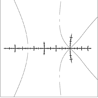
Figure 11. The Julia set of the cubic polynomial $f(z)=z^{3}-9/4z+\sqrt{3}/4$ and the external rays landing at the critical points.

Example: The polynomial $f(z)=z^{3}+0.2203+1.1863I$ has a unique critical point which is the landing point of the external rays with arguments

$$11/216,17/216,83/216,89/216,155/216,161/216.$$

Arguing as in the previous example, the cubic critical portraits

$$\{11/216,83/216,155/216\}$$

$$\{17/216,89/216,161/216\}$$

$$\{\{17/216,89/216\},\{11/216,155/216\}\}$$

$$\{\{89/216,161/216\},\{11/216,83/216\}\}$$

$$\{\{17/216,161/216\},\{83/216,155/216\}\}$$

have as impression the polynomial $f(z)=z^{3}+0.2203+1.1863I$. Notice that although $f$ has a unique multiple critical point there are critical portraits formed by two sets that generate the rational lamination of $f$.

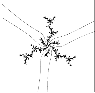
Figure 12. The Julia set of the cubic polynomial $f(z)=z^{3}+0.2203+1.1863I$ and the external rays landing at the critical point.

Note that the Mandelbrot local connectivity conjecture says that impressions of quadratic critical portraits are a single map. We would like to stress that, for higher degrees, we do not expect this to be true. That is, there might be non-trivial impressions of critical portraits with aperiodic kneading.

15. From ${\lambda_{{\mathbb{Q}}}}(f)$ to ${\Lambda_{{\mathbb{Q}}}}({\Theta})$

In this section we show that every rational lamination ${\lambda_{{\mathbb{Q}}}}(f)$ of a polynomial $f$ with all cycles repelling can be realized as ${\Lambda_{{\mathbb{Q}}}}({\Theta})$, for some critical portrait ${\Theta}$. Recall that, under the assumption that all cycles of $f$ are repelling, the rational lamination ${\lambda_{{\mathbb{Q}}}}(f)$ is a maximal equivalence relation with finite and unlinked classes (Proposition 11.4). Thus, the strategy is first to show that, for an arbitrary critical portrait ${\Theta}$, the equivalence relation ${\Lambda_{{\mathbb{Q}}}}({\Theta})$ has finite and unlinked classes (Lemma 15.1 below). Then we proceed to prove that ${\lambda_{{\mathbb{Q}}}}(f)\subset{\Lambda_{{\mathbb{Q}}}}({\Theta})$ for some critical portrait ${\Theta}$ (Proposition 15.2) and, by maximality of ${\lambda_{{\mathbb{Q}}}}(f)$ we conclude that ${\lambda_{{\mathbb{Q}}}}(f)={\Lambda_{{\mathbb{Q}}}}({\Theta})$.

Lemma 15.1.

Let $\Theta$ be a critical portrait.

Every ${\Lambda_{{\mathbb{Q}}}}({\Theta})$-equivalence class $A$ is a finite set.

If $A_{1}$ and $A_{2}$ are distinct ${\Lambda_{{\mathbb{Q}}}}({\Theta})$-equivalence classes then $A_{1}$ and $A_{2}$ are unlinked.

These properties of ${\Lambda_{{\mathbb{Q}}}}({\Theta})$ can be proven abstractly. Nevertheless, the intuition behind it is that there exists a polynomial $g$ in the visible shift locus whose rational external rays land in a pattern very closely related to that given by ${\Lambda_{{\mathbb{Q}}}}({\Theta})$ (Lemma 8.6). Our proof will make use of this fact:

Proof: Choose a polynomial $g$ in the visible shift locus with critical portrait $\Theta(g)=\Theta$.

To show that $A$ is finite we pick $t_{1}\in A$ and make a distinction according to whether $t_{1}$ is periodic or pre-periodic. In the case that $t_{1}$ is periodic of period $p$, it is enough to verify that all the elements of $A$ are periodic of period $p$. In fact, take $t_{2}\in A$ such that $\mathrm{itin}^{\epsilon_{1}}_{{\Theta}}(t_{1})=\mathrm{itin}^{\epsilon_{2}}_{{\Theta}}(t_{2})$ where $\epsilon_{1},\epsilon_{2}\in\{+,-\}$. In view of Lemma 8.6, the external rays $R^{t^{\epsilon}_{1}}_{g}$ and $R^{t^{\epsilon_{2}}_{2}}_{g}$ land at a periodic point $z$. By Theorem 2.2, both $t_{1}$ and $t_{2}$ have period $p$. It follows that all the elements of $A$ have the same period $p$. Now, in the case that $t_{1}$ is pre-periodic, say that $d^{l}t_{1}$ is periodic of period $p$. For each element $t\in A$, a similar argument shows that $d^{l}t$ is periodic of period $p$. Thus, $A$ is a finite set of pre-periodic arguments.

Now we must show that the ${\Lambda_{{\mathbb{Q}}}}({\Theta})$-equivalence classes $A_{1}$ and $A_{2}$ are unlinked. That is, $A_{2}$ is contained in a connected component of ${{\mathbb{R}}/{\mathbb{Z}}}\setminus A_{1}$. In fact, consider the union $\Gamma_{1}$ (resp. $\Gamma_{2}$) of all the external rays $R^{t^{\pm}}_{g}$ with arguments $t\in A_{1}$ (resp. $t\in A_{2}$) and their landing points. Observe that $\Gamma_{1}$ and $\Gamma_{2}$ are disjoint connected sets. Thus, $\Gamma_{2}$ is contained in a connected component of ${\mathbb{C}}\setminus\Gamma_{1}$. In the circle at infinity, it follows that $A_{2}$ is contained in a connected component of ${{\mathbb{R}}/{\mathbb{Z}}}\setminus A_{1}$. $\Box$

Now we characterize the critical portraits that generate a given rational lamination:

Proposition 15.2.

Consider a polynomial $f$ with connected Julia set $J(f)$ and all cycles repelling. Let ${\lambda_{{\mathbb{Q}}}}(f)$ be its rational lamination. Then there exists at least one and at most finitely many critical portraits $\Theta$ such that

$$\Lambda_{{\mathbb{Q}}}(\Theta)={\lambda_{{\mathbb{Q}}}}(f).$$

Moreover, all such critical portraits have aperiodic kneading. Furthermore, $\Theta=\{\Theta_{1},\dots,\Theta_{m}\}$ satisfies the identity above if and only if each ${\Theta}_{i}$ is either contained in a ${\lambda_{{\mathbb{Q}}}}(f)$-equivalence class or ${\Theta}_{i}$ is unlinked with all ${\lambda_{{\mathbb{Q}}}}(f)$-equivalence classes.

Proof of Proposition: Corollary 13.4 provides us with a critical portrait ${\Theta}=\{{\Theta}_{1},\dots,{\Theta}_{m}\}$ such that

(a) If ${\Theta}_{i}\subset{{\mathbb{Q}}/{\mathbb{Z}}}$ then ${\Theta}_{i}$ is contained in a ${\lambda_{{\mathbb{Q}}}}(f)$-equivalence class,

(b) If ${\Theta}_{i}\subset{{\mathbb{R}}/{\mathbb{Z}}}\setminus{{\mathbb{Q}}/{\mathbb{Z}}}$ then ${\Theta}_{i}$ is unlinked with all ${\lambda_{{\mathbb{Q}}}}(f)$-equivalence classes.

We show that these are sufficient conditions to conclude that ${\lambda_{{\mathbb{Q}}}}(f)={\Lambda_{{\mathbb{Q}}}}({\Theta})$.

Consider an arbitrary ${\lambda_{{\mathbb{Q}}}}(f)$-equivalence class $A$ and let $t_{1},t_{2}$ be two consecutive elements of $A$. That is, $(t_{1},t_{2})$ is a connected component of ${{\mathbb{R}}/{\mathbb{Z}}}\setminus A$. Observe that (a) and (b) guarantee that the first symbol of $\mathrm{itin}^{+}_{{\Theta}}(t_{1})$ coincides with the first symbol of $\mathrm{itin}^{-}_{{\Theta}}(t_{2})$. In view of property (R4) of ${\lambda_{{\mathbb{Q}}}}(f)$ in Proposition 11.4, $d^{n}t_{1}$ and $d^{n}t_{2}$ are consecutive elements of $m^{\circ n}_{d}(A)$. Thus, $\mathrm{itin}^{+}_{{\Theta}}(t_{1})=\mathrm{itin}^{-}_{{\Theta}}(t_{2})$ and $A$ is contained in a ${\Lambda_{{\mathbb{Q}}}}({\Theta})$-equivalence class. That is, ${\lambda_{{\mathbb{Q}}}}(f)\subset{\Lambda_{{\mathbb{Q}}}}({\Theta})$. Now Proposition 11.4 says that ${\lambda_{{\mathbb{Q}}}}(f)$ is a maximal equivalence relation with finite and unlinked classes. By Lemma 15.1, we conclude ${\lambda_{{\mathbb{Q}}}}(f)={\Lambda_{{\mathbb{Q}}}}({\Theta})$

Assume that ${\lambda_{{\mathbb{Q}}}}(f)={\Lambda_{{\mathbb{Q}}}}({\Theta})$, we must prove that the conditions (a) and (b) hold. By contradiction, suppose that ${\Theta}_{i}$ lies in ${{\mathbb{Q}}/{\mathbb{Z}}}$ and it is not contained in a ${\lambda_{{\mathbb{Q}}}}(f)$-class. By Lemma 13.1, ${\Theta}_{i}$ is linked with infinitely many ${\lambda_{{\mathbb{Q}}}}(f)$-classes. A class of ${\Lambda_{{\mathbb{Q}}}}({\Theta})$ which is linked with ${\Theta}_{i}$ must contain an element of ${\Theta}_{i}$. Therefore, ${\Lambda_{{\mathbb{Q}}}}({\Theta})$ would have an infinite class. This contradicts Lemma 15.1 and implies that (a) holds. If ${\Theta}_{i}$ lies in ${{\mathbb{R}}/{\mathbb{Z}}}\setminus{{\mathbb{Q}}/{\mathbb{Z}}}$, Lemma 13.3 allows us to apply a similar reasoning to show that ${\Theta}_{i}$ is unlinked with every ${\lambda_{{\mathbb{Q}}}}(f)$-class.

To show that a critical portrait ${\Theta}$ such that ${\lambda_{{\mathbb{Q}}}}(f)={\Lambda_{{\mathbb{Q}}}}({\Theta})$ must have aperiodic kneading, consider a polynomial $g$ in the visible shift locus such that ${\Theta}={\Theta}(g)=\{{\Theta}_{1},\dots,{\Theta}_{m}\}$. No periodic $t\in{{\mathbb{Q}}/{\mathbb{Z}}}$ participates in ${\Theta}$, otherwise some ${\Theta}_{i}$ contains periodic and pre-periodic arguments and cannot be contained in a ${\lambda_{{\mathbb{Q}}}}(f)$-class as proved above. Thus, all the periodic rays of $g$ are smooth. Since ${\lambda_{{\mathbb{Q}}}}(f)={\Lambda_{{\mathbb{Q}}}}({\Theta})$, if $A\subset{{\mathbb{Q}}/{\mathbb{Z}}}$ is a periodic point type of $f$ then $A$ is a periodic point type of $g$. Thus, $g$ has exactly $d^{p}$ rational periodic point types of period dividing $p$. This matches with the $d^{p}$ periodic points of $g$ of period dividing $p$. Therefore, no ray that bounces off a critical point of $g$ can land at a periodic point of $g$. It follows that ${\Theta}(g)={\Theta}$ has aperiodic kneading. $\Box$

Lemma 15.3.

Consider a critical portrait ${\Theta}=\{{\Theta}_{1},\dots,{\Theta}_{m}\}$ such that all the arguments in ${\Theta}_{1}\cup\dots\cup{\Theta}_{m}$ are strictly pre-periodic. If $f$ is a polynomial such that ${\lambda_{{\mathbb{Q}}}}(f)={\Lambda_{{\mathbb{Q}}}}({\Theta})$ then all the critical points of $f$ are strictly pre-periodic.

Proof: It is not difficult to check that ${\Theta}$ has aperiodic kneading. A counting argument as above shows that $f$ has all cycles repelling. Proposition 15.2 implies that the external rays with arguments in ${\Theta}_{i}$ land at a common critical point. Counting multiplicities, it follows that all the critical points of $f$ are the landing point of some ${\Theta}_{i}$. Thus, $f$ is a critically pre-repelling map. $\Box$

16. Critical Portraits with
aperiodic kneading

In the next section we are going to show that polynomials $f$ in the impression $I_{{{\mathcal{C}}_{d}}}({\Theta})$ of a critical portrait ${\Theta}$ with aperiodic kneading has all cycles repelling. A key step in the proof is to rule out parabolic cycles of $f$. To do so we will show that two periodic points cannot coalesce as one goes from the shift locus to the connectedness locus in the “direction” determined by ${\Theta}$. Roughly, the obstruction for this collision to occur is that, for polynomials in ${{\mathcal{S}}^{vis}_{d}}$ with critical portrait ${\Theta}$, any two periodic points are separated by the external rays landing at a pre-periodic point (see Figure 13):

Lemma 16.1 (Separation).

Consider a critical portrait $\Theta$ with aperiodic kneading and let $A_{1}$ and $A_{2}$ be two distinct periodic ${\Lambda_{{\mathbb{Q}}}}(\Theta)$-equivalence classes. Then there exists a strictly pre-periodic ${\Lambda_{{\mathbb{Q}}}}({\Theta})$-equivalence class $C$ such that $A_{1}$ and $A_{2}$ lie in different connected components of ${{\mathbb{R}}/{\mathbb{Z}}}\setminus C$. Moreover, $C$ can be chosen such that, for all $n\geq 0$, $m^{\circ n}_{d}(C)$ is contained in a ${\Theta}$-unlinked class.

Figure 13. The diagram illustrates the situation of Lemma 16.1.

Note that for ${\Theta}^{\prime}$ close to ${\Theta}$ each of the sets $A_{1}$, $A_{2}$ and $C$ is also contained in a ${\Lambda_{{\mathbb{Q}}}}({\Theta}^{\prime})$-equivalence class.

The idea of the proof is similar to that of Lemma 13.1:

Proof: Pick a polynomial $f$ in the visible shift locus with critical portrait ${\Theta}={\Theta}(f)$. Observe that since ${\Theta}$ has aperiodic kneading all the external rays landing at periodic points are rational and smooth. Moreover, the periodic point types of $f$ are exactly the periodic equivalence classes of ${\Lambda_{{\mathbb{Q}}}}({\Theta})$. Let $z_{1},z_{2}$ be such that $A_{1}=A(z_{1})$ and $A_{2}=A(z_{2})$. The idea is to construct, with smooth rays, a puzzle piece around $z_{1}$ which does not contain $z_{2}$. For this, consider the collection $\mathcal{G}$ formed by the rational typess $A(w)$ such that:

(i) All the external rays landing at a point in the grand orbit of $w$ are smooth.

(ii) $w$ is not in the grand orbit of $z_{1}$.

We pass to an iterate of $f$ so that every periodic point $w$ whose type does not lie in $\mathcal{G}$ is a fixed point and all the rays landing at $w$ are fixed rays. In particular, now $z_{1}$ is a fixed point which is the landing point of fixed rays.

We saturate $\mathcal{G}$ by an increasing sequence of finite collections $G_{l}$. That is, let $G_{l}$ be the collection of types $A(w)$ in $\mathcal{G}$ such that $f^{\circ l}(w)$ is periodic of period less or equal to $l$. Let $U_{l}(z_{1})$ be the $G_{l}$-puzzle piece which contains $z_{1}$.

It is enough to show that, for some $l$, $f$ maps $U_{l}(z_{1})$ homeomorphically onto its image. We suppose that this is not the case and, after some work, we arrive to a contradiction. That is, suppose that for $l\geq l_{0}$ the map $f_{|U_{l}}(z_{1})$ has degree $k>1$. We can pick $l_{0}$ large enough so that every fixed point in $\overline{U}_{l_{0}}(z_{1})$ is the landing point of fixed external rays.

Claim 1: For $l\geq l_{0}$, $f$ has $k$ fixed points in $\overline{U}_{l}(z_{1})$.

Proof of Claim 1: Let $\rho>0$ be large enough such that the equipotential $g_{f}=\rho$ is a topological circle (i.e. all the critical points of $f$ are contained inside $g_{f}=\rho$). Consider the portion $U$ of $U_{l}(z_{1})$ contained inside this equipotential. Let $U^{\prime}=f(U)$. Observe that $U$ and $U^{\prime}$ are puzzle pieces that satisfy the conditions of the thickening Lemma 12.5. The same construction shows that, after extracting a polynomial like map of degree $k$, we must have $k$ fixed points of $f$ in $\overline{U}_{l}(z)$.

Now let $V_{n}$ be the connected component of $f^{-n}(U_{l_{0}}(z_{1}))$ that contains $z_{1}$ and

$$X=\cap_{n\geq 0}f^{-n}(\overline{V_{n}}).$$

In the circle at infinity, let $\pi_{\infty}V_{n}=\{t\in{{\mathbb{R}}/{\mathbb{Z}}}:R^{*t}_{f}\subset V_{n}\}$ and

$$E=\cap_{n\geq 0}\overline{\pi_{\infty}{V_{n}}}.$$

Observe that $m_{d}$ is $k$ to $1$ on $E$. Moreover, $E$ contains elements of $k$ distinct fixed point types formed by fixed rays. Our aim is to show that $E$ can only intersect $k-1$ fixed point types which are formed by fixed arguments. Roughly speaking, we will construct a semiconjugacy between $m_{d}|_{E}$ and a degree $k$ selfcovering of a circle. For this, we need some basic facts about $E$.

Claim 2: If $(t_{1},t_{2})$ is a connected component of ${{\mathbb{R}}/{\mathbb{Z}}}\setminus E$ then $(dt_{1},dt_{2})$ is also a connected component of ${{\mathbb{R}}/{\mathbb{Z}}}\setminus E$. Moreover, the external rays $R^{t^{+}_{1}}_{f}$ and $R^{t^{-}_{2}}_{f}$ land at the same point.

Proof of Claim 2: Notice $(t_{1},t_{2})=\cup_{n\geq 1}(a_{n},b_{n})$ where $(a_{n},b_{n})$ is a connected component of ${{\mathbb{R}}/{\mathbb{Z}}}\setminus\overline{\pi_{\infty}V}_{n}$. Since $a_{n},b_{n}$ are rational and $f$ acts preserving the cyclic order of the rational rays that bound $V_{n}$ we have that $(da_{n},db_{n})$ is a connected component of ${{\mathbb{R}}/{\mathbb{Z}}}\setminus\overline{\pi_{\infty}V}_{n-1}$. Thus, $(t_{1},t_{2})$ is a connected component of ${{\mathbb{R}}/{\mathbb{Z}}}\setminus E$. Since the ${\Theta}$-itineraries of $a_{n}$ and $b_{n}$ agree, $R^{t^{+}_{1}}_{f}$ and $R^{t^{-}_{2}}_{f}$ land at the same point.

Also, we need some control over the (possibly) isolated points of $E$:

Claim 3: Let $\{t_{i}\}\subset E$ such that $(t_{i},t_{i+1})$ is a connected component of ${{\mathbb{R}}/{\mathbb{Z}}}\setminus E$. Then $\{t_{i}\}$ is finite.

Proof of Claim 3: There are two possibilities. In the case that there is a rational $t_{i_{1}}\in\{t_{i}\}$, then $R^{t^{+}_{i_{1}}}$ lands at a pre-periodic or periodic point $z$. The previous Claim implies that the external ray $R^{t^{-}_{i_{1}+1}}_{f}$ also lands at $z$. Hence, $t_{i_{1}+1}$ is rational and it is ${\Lambda_{{\mathbb{Q}}}}({\Theta})$-equivalent to $t_{i_{1}}$. It follows that all the elements of $\{t_{i}\}$ are ${\Lambda_{{\mathbb{Q}}}}({\Theta})$-equivalent. Since ${\Lambda_{{\mathbb{Q}}}}({\Theta})$-classes are finite, we conclude that $\{t_{i}\}$ is finite.

If all the elements of $\{t_{i}\}$ are irrational and this set is infinite then there exists two elements $t_{j},t_{j+l}$ such that $d^{k_{1}}t_{j}=d^{k_{2}}t_{j+l}=\theta$ where $\theta\in{\Theta}_{1}\cup\cdots\cup{\Theta}_{m}$ and $k_{1}\neq k_{2}$. For $n$ large enough, all the rays with arguments $d^{n}t_{j},d^{n}t_{j+1},\dots,d^{n}t_{j+l}$ are smooth. By the previous Claim, all these rays must land at the same point $z$. It follows that the external rays with arguments $d^{n-k_{1}}\theta$ and $d^{n-k_{2}}\theta$ land at the same point $z$. Since $k_{1}\neq k_{2}$ we have that $z$ must be periodic. Thus, $\theta\in{{\mathbb{Q}}/{\mathbb{Z}}}$ and $t_{j}$ must also be rational. Which puts us in the first case.

It follows that the set $\tilde{E}$ obtained by removing from $E$ its isolated points is a Cantor set. Moreover, if $(t_{1},t_{2})$ is a connected component of ${{\mathbb{R}}/{\mathbb{Z}}}\setminus\tilde{E}$ then $(dt_{1},dt_{2})$ is also a connected component of ${{\mathbb{R}}/{\mathbb{Z}}}\setminus\tilde{E}$. Every fixed point type that had an element in $E$ also has an element in $\tilde{E}$. Furthermore, ${m_{d}}_{|\tilde{E}}$ is $k$ to $1$.

Now consider the quotient ${\mathbb{T}}$ obtained from ${{\mathbb{R}}/{\mathbb{Z}}}$ by identifying $[t_{1},t_{2}]$ to a point if and only if $(t_{1},t_{2})$ is a connected component of ${{\mathbb{R}}/{\mathbb{Z}}}\setminus\tilde{E}$. Let

$$h:{{\mathbb{R}}/{\mathbb{Z}}}\rightarrow{{\mathbb{T}}}$$

be the quotient map. It follows that $m_{d}$ projects to a degree $k$ selfcovering $g$ of the topological circle ${\mathbb{T}}$. Moreover, each fixed point of $g$ is either the image of a fixed point $t$ of $m_{d}$ or of an interval $[t_{1},t_{2}]$ whose endpoints are fixed points of $m_{d}$. Observe that, in the latter case, $R^{t_{1}}_{f}$ and $R^{t_{2}}_{f}$ land at the same fixed point of $f$. Therefore, $h$ does not identify arguments of distinct fixed point types that have elements in $\tilde{E}$. Recall that there are $k$ fixed point types with rotation number zero that have elements in $\tilde{E}$. Thus, $g$ has at least $k$ fixed points. But, every fixed point of $g$ is topologically repelling. Thus, $g$ has $k-1$ fixed points. Contradiction. $\Box$

The previous Lemma says that periodic points are separated by smooth pre-periodic rays. The next Lemma will allow us to show that this separation persists in the limit when we go from the shift locus ${{\mathcal{S}}_{d}}$ to the connectedness locus ${{\mathcal{C}}_{d}}$.

In order to make this precise, we consider a sequence of external rays $R^{t}_{f_{n}}$ and say that

$$\limsup R^{t}_{f_{n}}$$

is the set of points $z\in{\mathbb{C}}$ such that every neighbourhood of $z$ intersects infinitely many $R^{t}_{f_{n}}$. This coincides with the usual definition of the Hausdorff metric on compact subsets of the Riemann sphere.

Lemma 16.2.

Let ${\Theta}$ be a critical portrait with aperiodic kneading. Consider a sequence $f_{n}\in{{\mathcal{S}}^{vis}_{d}}$ such that ${\Theta}(f_{n})\rightarrow{\Theta}$ and $f_{n}\rightarrow f\in{{\mathcal{C}}_{d}}$.

If $t\in{{\mathbb{Q}}/{\mathbb{Z}}}$ is periodic and $z\in\limsup R^{t}_{f_{n}}\cap J(f)$ then $z$ is periodic under $f$.

If $t\in{{\mathbb{Q}}/{\mathbb{Z}}}$ is such that $t$ is not periodic and $z\in\limsup R^{t^{\pm}}_{f_{n}}\cap J(f)$ then $z$ is not periodic under $f$.

Proof: Assume $t$ is periodic of period $p$. Since ${\Theta}$ has aperiodic kneading, for $n$ sufficiently large, $R^{t}_{f_{n}}$ is smooth.

Claim 1: Consider $z_{n}\in R^{t}_{f_{n}}$, we claim that, for $n$ large enough,

$$\rho_{\Omega(f_{n})}(z_{n},f^{\circ p}_{n}(z_{n}))<2p\log d$$

where $\rho_{\Omega(f_{n})}$ is the hyperbolic metric in $\Omega(f_{n})$.

Let us postpone this estimate and proceed with the proof. If

$$z\in\limsup R^{t}_{f_{n}}\cap J(f)$$

then consider a sequence $z_{n}\in R^{t}_{f_{n}}$ which converges to $z$. Since repelling cycles of $f$ are dense in $J(f)$, the euclidean distance between $z_{n}$ and $J(f_{n})=\partial\Omega(f_{n})$ goes to zero. In the other hand, the hyperbolic distance between $z_{n}$ and $f^{\circ p}_{n}(z_{n})$ stays bounded. The standard comparison between the hyperbolic metric and the euclidean metric yields that $z_{n}$ and $f^{\circ p}_{n}(z_{n})$ must converge to the same point $z$. It follows that $f^{\circ p}(z)=z$, i.e. $z$ is periodic.

Now, in the case that $t\in{{\mathbb{Q}}/{\mathbb{Z}}}$ is strictly pre-periodic and we first consider the case in which $dt$ is a periodic argument. If $w\in\limsup R^{t^{\pm}}_{f_{n}}\cap J(f)$ then we proved that $f(w)$ must be periodic. There are two possibilities, either $w$ is the unique periodic preimage of $f(w)$ or $w$ is strictly pre-periodic. We claim that only the latter occurs. By contradiction, suppose that $w$ is periodic. Let $w_{n}\in R^{t^{\pm}}_{f_{n}}$ be such that $w_{n}\rightarrow w$ and $t^{\prime}\in{{\mathbb{Q}}/{\mathbb{Z}}}$ be the unique periodic preimage of $t$. Consider $w^{\prime}_{n}\in R^{t^{\prime}}_{f}$ such that $f_{n}(w^{\prime}_{n})=f_{n}(w_{n})$. Since $t^{\prime}$ is periodic, $w^{\prime}_{n}$ must converge to the unique periodic pre-image $w$ of the periodic point $f(w)$. Thus, $f$ is not locally injective at $w$, but $w$ is a periodic point in the Julia set $J(f)$. Contradiction. The general case, for an arbitrary strictly pre-periodic $t$, follows.

Proof of Claim 1: The estimate will follow from Lemma 8.7. Let $H=\{z=x+iy:x>0\}$ and consider the region $\tilde{V}=2\pi it+\{z\in H:|\arg z|<\pi/4\}$. By Lemma 8.7, for $n$ sufficiently large, $exp(\tilde{V})\subset U_{f_{n}}$, where $U_{f_{n}}$ is the image of the Böttcher map $\phi_{f_{n}}:\Omega^{*}(f_{n})\rightarrow U_{f_{n}}$. Observe that:

$$z_{n}=\phi^{-1}_{f_{n}}\circ exp(g_{f_{n}}(z_{n})+2\pi it)$$

$$f^{\circ p}_{n}(z_{n})=\phi^{-1}_{f_{n}}\circ exp(d^{p}g_{f_{n}}(z_{n})+2\pi it).$$

Also,

$$\rho_{\tilde{V}}(g_{f_{n}}(z_{n})+2\pi it,d^{p}g_{f_{n}}(z_{n})+2\pi it)=2p\log d$$

where $\rho_{\tilde{V}}$ is the hyperbolic metric in $\tilde{V}$. Since, $\phi^{-1}_{f_{n}}\circ exp$ is a contraction the Claim follows. $\Box$

17. Combinatorial Continuity

Before we prove Theorem 14.4 we need the following Lemma due to Goldberg and Milnor [GM]:

Lemma 17.1.

Consider $f_{0}\in{{\mathcal{P}}_{d}}$ such that $J(f_{0})$ is connected. Assume that $R^{t}_{f_{0}}$ is a smooth external ray which lands at a pre-repelling or repelling periodic point $z_{f_{0}}$. Also, assume that $z_{f_{0}}$ is not a pre-critical point. Then, for any $f$ sufficiently close to $f_{0}$, the external ray $R^{t}_{f}$ is smooth and lands at the analytic continuation $z_{f}$ of $z_{f_{0}}$.

Proof of Theorem 14.4: Consider a critical portrait ${\Theta}$ with aperiodic kneading and a polynomial $f$ in its impression $I_{{{\mathcal{C}}_{d}}}({\Theta})$. So let $f_{n}$ be a sequence in the visible shift locus such that:

$$f_{n}\rightarrow f$$

$${\Theta}(f_{n})\rightarrow{\Theta}.$$

The next two claims show that $f$ must have all cycles repelling:

Claim 1: $f$ does not have a parabolic cycle.

Proof of Claim 1: By contradiction, suppose that $z$ is a parabolic periodic point of $f$. It follows that there exists distinct repelling periodic points $z_{1}(n)$ and $z_{2}(n)$ of $f_{n}$ that converge to $z$. Also, the periods of $z_{1}(n)$ and $z_{2}(n)$ divide a fixed number $p$. Since ${\Theta}$ has aperiodic kneading the itinerary of periodic elements of ${{\mathbb{Q}}/{\mathbb{Z}}}$ vary continuously. In particular, for ${\Theta}^{\prime}$ in a sufficiently small neighbourhood of ${\Theta}$ the periodic classes of ${\Lambda_{{\mathbb{Q}}}}({\Theta})$ with period dividing $p$ coincide with those of ${\Lambda_{{\mathbb{Q}}}}({\Theta}^{\prime})$. After passing to a subsequence, we may assume that the type of $z_{1}(n)$ is $A_{1}$ and the type of $z_{2}(n)$ is $A_{2}$, where $A_{1}$ and $A_{2}$ are distinct equivalence classes of ${\Lambda_{{\mathbb{Q}}}}({\Theta})$. By Lemma 16.1 we know that there exists a strictly pre-periodic class $C$ of ${\Lambda_{{\mathbb{Q}}}}({\Theta})$ such that it separates $A_{1}$ and $A_{2}$ (i.e. $A_{1}$ and $A_{2}$ lie in different connected components of ${{\mathbb{R}}/{\mathbb{Z}}}\setminus C$). Recall that none of the elements of $C$ and its forward orbit participate of ${\Theta}$. Hence, for ${\Theta}^{\prime}$ in a sufficiently small neighborhood of ${\Theta}$, the elements of $C$ are also identified by ${\Lambda_{{\mathbb{Q}}}}({\Theta}^{\prime})$. Thus, for $n$ large the external rays of $f_{n}$ with arguments in $C$ together with their landing points form a connected set $\Gamma_{n}$. Now the periodic points $z_{1}(n)$ and $z_{2}(n)$ lie in different connected components of ${\mathbb{C}}\setminus\Gamma_{n}$. Passing to the limit, $z\in\limsup\Gamma_{n}$ and therefore $z\in\limsup R^{t}_{f_{n}}$, for some $t\in C$. This contradicts Lemma 16.2 and shows that $f$ cannot have parabolic cycles.

Claim 2: $f$ does not have irrationally neutral cycles.

Proof of Claim 2: Again by contradiction we suppose that $z$ is an irrationally neutral periodic point of $f$ with period $p$. There exists a sequence $z(n)$ of periodic points of $f_{n}$ that converge to $z$. As above, after passing to a subsequence, we may assume that $z(n)$ has type $A\subset{{\mathbb{Q}}/{\mathbb{Z}}}$, for all $n$. Pick an element of $t\in A$ and notice that $R^{t}_{f}$ must land at a repelling periodic point $w$. Hence, for $n$ large enough, $R^{t}_{f_{n}}$ has to land in the analytic continuation of $w$ which is not $z(n)$.

Claim 3: If $f$ is a polynomial with all cycles repelling and $f\in I_{{{\mathcal{C}}_{d}}}({\Theta})$ for some critical portrait ${\Theta}\in{\mathcal{A}}_{d}$ then ${\Lambda_{{\mathbb{Q}}}}({\Theta})={\lambda_{{\mathbb{Q}}}}(f)$.

It follows from Proposition 15.2 that ${\Theta}$ has aperiodic kneading.

Proof of Claim 3: Consider $f_{n}$ in the visible shift locus such that

$$f_{n}\rightarrow f$$

and

$${\Theta}(f_{n})\rightarrow{\Theta}=\{{\Theta}_{1},\dots,{\Theta}_{m}\}$$

Now we show that each ${\Theta}_{i}$ is either contained in a ${\lambda_{{\mathbb{Q}}}}(f)$-class or it is unlinked with all ${\lambda_{{\mathbb{Q}}}}(f)$-classes. If ${\Theta}_{i}$ has elements in two distinct equivalence classes of ${\lambda_{{\mathbb{Q}}}}(f)$ then ${\Theta}_{i}$ is linked with the rational type $A(w)$ of a point $w$ which is not in the grand orbit of a critical point. For ${\Theta}^{\prime}$ close to ${\Theta}$, we also have that $C=A(w)$ has points in two different ${\Theta}^{\prime}$-unlinked classes. In view of Lemma 17.1, for $n$ large enough, the external rays of $f_{n}$ with arguments in $C$ are smooth and land at a common point. Therefore, they intersect the external radii of $f_{n}$ terminating at some critical point. This is impossible. A similar situation occurs when ${\Theta}_{i}\subset{{\mathbb{R}}/{\mathbb{Z}}}\setminus{{\mathbb{Q}}/{\mathbb{Z}}}$ is linked with a ${\lambda_{{\mathbb{Q}}}}(f)$-class. By Proposition 15.2, ${\Lambda_{{\mathbb{Q}}}}({\Theta})={\lambda_{{\mathbb{Q}}}}(f)$. $\Box$

Theorem 14.3 follows from Theorem 14.4 and Proposition 15.2.

Corollary 17.2.

Assume ${\Theta}=\{{\Theta}_{1},\dots,{\Theta}_{m}\}$ is a critical portrait formed by strictly pre-periodic arguments. Then the critical portrait impression $I_{{{\mathcal{C}}_{d}}}({\Theta})$ is formed by the unique critically pre-repelling polynomial $f$ such that, for each ${\Theta}_{i}$, the external rays with arguments in ${\Theta}_{i}$ land at a common critical point.

Proof: By Theorem 14.4 and Lemma 15.3, each polynomial $f$ in the impression $I_{{{\mathcal{C}}_{d}}}({\Theta})$ is critically pre-repelling and such that ${\lambda_{{\mathbb{Q}}}}(f)={\Lambda_{{\mathbb{Q}}}}({\Theta})$. According to Proposition 15.2, this occurs if and only if the external rays with arguments in ${\Theta}_{i}$ land at same point. As mentioned above it follows from the work of Jones [J] or the work of Bielefield, Fisher and Hubbard [BFH] that $f$ is uniquely determined by its rational lamination ${\Lambda_{{\mathbb{Q}}}}({\Theta})$. $\Box$

This paper is a copy of the author’s Ph. D. Thesis produced at the Mathematics Deparment, S.U.N.Y. at Stony Brook, U.S.A.

Current Address:

Facultad de Matemáticas,

Pontitificia Universidad Católica de Chile.

Casilla 306, Correo 22, Santiago,

Chile.

jkiwi@riemann.mat.puc.cl

References

- [Ah] L. V. Ahlfors. Lectures on Quasiconformal Mappings. Princeton University Press, Van Nostrand.
- [At] P. Atela. Bifurcations of dynamic rays in complex polynomials of degree two. Ergodic Th. and Dyn. Sys., 12:401–423, 1992.
- [BDK] P. Blanchard, R.L. Devaney, and L. Keen. The dynamics of complex polynomials and automorphism of the shift. Invent. Math, 104:545–580, 1991.
- [BFH] B. Bielifield, Y. Fisher, and J. H. Hubbard. The classification of critically preperiodic polynomials as dynamical systems. Journal AMS, 5:721–762, 1992.
- [BH] B. Branner and J. H. Hubbard. The iteration of cubic polynomials. part I: The global topology of parameter space. Acta Math., 160:143 –206, 1988.
- [BL] B. Bielefield and M. Lyubich. Problems in holomorphic dynamics. In Linear and complex analysis problem book, volume III. Springer, 1994.
- [Bl] P. Blanchard. Complex analytic dynamics in the Riemann sphere. Bull. AMS, 11:85–141, 1984.
- [CG] L. Carlesson and T. W. Gamelin. Complex Dynamics. Springer-Verlag, 1993.
- [DH0] A. Douady and J. H. Hubbard. Itération des polynomes quadratiques complexes. C. R. Acad. Sci. Paris Ser. I Math., 294:123–126, 1982.
- [DH1] A. Douady and J. H. Hubbard. Étude dynamique des polynomes complexes I, II. Publ. Math. Orsay, 1984 - 1985.
- [DH2] A. Douady and J. H. Hubbard. A proof of Thurston’s characterization of rational functions. Acta Math., 171:263–297, 1993.
- [D] A. Douady. Description of compact sets in C. In Topological Methods in Modern Mathematics. Publish or Perish, 1993.
- [F] Y. Fisher. -. PhD thesis, Cornell, 1989.
- [GM] L. R. Goldberg and J. Milnor. Fixed points of polynomial maps II: Fixed point portraits. Ann. Scient. École Norm. Sup., série, 26:51–98, 1993.
- [G] L. R. Goldberg. On the multiplier of a repelling fixed point. Invent. Math, pages 85–108, 1994.
- [H] J. H. Hubbard. Local connectivity of Julia sets and bifurcation loci: three theorems of J.-C. Yoccoz. In Topological Methods in Modern Mathematics. Publish or Perish, 1993.
- [J] P. Jones. On removable sets for Sobolev spaces in the plane. Stony Brook IMS Preprint 1991/22.
- [La] P. Lavaurs. Une description combinatoire de l’involution definie par M sur les rationneles à dénominateur impair. C.R. Acad. Sci. Paris (4), 303:143–146, 1986.
- [La] P. Lavaurs. Systemes dynamiques holomorphes: explosion de points périodiques paraboliques. PhD thesis, Université Paris-Sud, 1989.
- [LP] G. Levin and F. Przytycki. External rays to periodic points. to appear in Isarael Math. Journal.
- [LS] G. Levin and M. Sodin. Polynomials with disconnected julia sets and green maps. Preprint No 23, The Hebrew University of Jerusalem, 1991.
- [LV] O. Lehto and K. J. Virtanen. Quasiconformal Mappings in the Plane. Springer-Verlag, 1973.
- [McM] C. T. McMullen. Complex Dynamics and Renormalization. Princeton University Press, 1994.
- [M1] J. Milnor. Dynamics in one complex variable: Introductory lectures. Stony Brook IMS Preprint 1990/5.
- [M2] J. Milnor. Periodic orbits, external rays and the Mandelbrot set. Manuscript, 1995.
- [P] A. Poirier. On postcritically finite polynomials, parts I, II. Stony Brook IMS Preprint 1993/5 and 7.
- [Sch] D. Schleicher. Internal addresses in the Mandelbrot set and irreducibility of polynomials. PhD thesis, Cornell, 1994.
- [Th] W. P. Thurston. On the combinatorics of iterated rational maps. Manuscript, 1985.