Geography of the Cubic Connectedness Locus I: Intertwining Surgery

Stony Brook IMS Preprint #1996/10 August 1996

1. Introduction

The prevalence of Mandelbrot sets in one-parameter complex analytic families is a well-studied phenomenon in conformal dynamics. Its explanation gave rise to the theory of renormalization [DH2], and subsequent efforts to invert this procedure by means of surgery on quadratic polynomials [BD, BF].

In this paper we exhibit products of Mandelbrot sets in the two-dimensional complex parameter space of cubic polynomials. These products were observed by J. Milnor in computer experiments which inspired Lavaurs’ proof of non local-connectivity for the cubic connectedness locus [La]. Cubic polynomials in such a product may be renormalized to produce a pair of quadratic maps. The inverse construction is an intertwining surgery on two quadratics. The idea of intertwining first appeared in a collection of problems edited by Bielefeld [Bi2]. Using quasiconformal surgery techniques of Branner and Douady [BD], we show that any two quadratics may be intertwined to obtain a cubic polynomial. The proof of continuity in our two-parameter setting requires further considerations involving ray combinatorics and a pullback argument.

After this project was finished, we were informed by P. Haissinsky that he is independently working on related problems [Haï].

Acknowledgments: This paper was motivated by J. Milnor’s Autumn 1995 Stony Brook lectures on the dynamics of cubic polynomials, and developed out of joint meditation of the two authors in front of the the full-color version of Fig. 2. We thank J. Milnor for numerous discussions of our results and many helpful suggestions as this paper progressed. We are indebted to M. Lyubich for fruitful conversations concerning various aspects of quadratic dynamics. Further thanks are due to J. Kiwi for sharing his understanding of cubic maps and discussing some of his current work, and to X. Buff for communicating his results. This project was conducted in the congenial atmosphere of IMS at Stony Brook, and we thank our colleagues for their interest and moral support.

The computer pictures in this paper were produced using software written by J. Milnor and S. Sutherland.

2. Preliminaries

In this section we discuss the relevant facts and tools of holomorphic dynamics. We assume that the reader is familiar with the basic notions and principles of the theory of quasiconformal maps (see [LV] for a comprehensive account). The knowledgeable reader is invited to proceed directly to §3.

2.1. Polynomial dynamics

Julia sets, external rays, landing theorems, combinatorial rotation number, Yoccoz Inequality

We recall the basic definitions and results in the theory of polynomial dynamics. Supporting details may be found in [Mil1].

Let $P:{\mathbb{C}}\to{\mathbb{C}}$ be a complex polynomial of degree $d\geq 2$. The filled Julia set of $P$ is defined as

$$K(P)=\{z\in{\mathbb{C}}|\{P^{\circ n}(z)\}\operatorname{is\;bounded}\}$$

and the Julia set as $J(P)=\partial K(P)$. Both of these are nonempty compact sets which are connected if and only all critical points of $P$ have bounded orbits.

Recall that if $P$ is a monic polynomial with connected Julia set then there exists a unique analytic homeomorphism (the Böttcher map)

$$B_{P}:{\mathbb{C}}\setminus K(P)\to{\mathbb{C}}\setminus\bar{{\mathbb{D}}}$$

which is tangent to the identity at infinity, that is $B_{P}(z)/z\to 1$ as $z\to\infty$. The Böttcher map conjugates $P$ to $z\mapsto z^{d}$,

$$B_{P}(P(z))=(B_{P}(z))^{d},$$

thereby determining a dynamically natural polar coordinate system on ${\mathbb{C}}\setminus K(P)$. For $\rho>1$ the equipotential $E_{\rho}$ is the inverse image under $B_{P}$ of the circle $\{\rho e^{2\pi i\theta}|\theta\in{{\mathbb{R}}}\}$. The external ray at angle $\theta$ is similarly defined as the inverse image $r_{\theta}$ of the radial line $\{\rho e^{2\pi i\theta}|\rho>1\}$. Since $P$ maps $r_{\theta}$ to $r_{d\cdot\theta}$, the ray $r_{\theta}$ is periodic if and only if the angle $\theta$ is periodic (mod $1$) under multiplication by $d$. An external ray $r_{\theta}$ is said to land at a point $\zeta\in J(P)$ when

$$\lim_{\rho\to 1}B_{P}^{-1}(\rho e^{2\pi i\theta})=\zeta.$$

We note that if the Julia set of $P$ is locally connected then all rays $r_{\theta}$ land, and their endpoints depend continuously on the angle $\theta$ (see the discussion in [Mil1]). We refer to [Mil1] for the proofs of the following results:

Theorem 2.1 (Sullivan, Douady and Hubbard).

If K(P) is connected, then every periodic external ray lands at a periodic point which is either repelling or parabolic.

Theorem 2.2 (Douady, Yoccoz).

If $K(P)$ is connected, every repelling or parabolic periodic point is the landing point of at least one external ray which is necessarily periodic.

The landing points of such rays depend continuously on parameters:

Lemma 2.3 ([GM]).

Let $P_{t}$ be a continuous family of monic degree $d$ polynomials with continuously chosen repelling periodic points $\zeta_{t}$. If the ray of angle $\theta$ for $P_{t_{0}}$ lands at $\zeta_{t_{0}}$, then for all $t$ close to $t_{0}$ the ray of angle $\theta$ for $P_{t}$ lands at $\zeta_{t}$.

Kiwi has proved the following useful separation principle which directly illustrates why a degree $d$ polynomial admits at most $d-1$ non-repelling periodic orbits; the latter result was earlier shown by Douady and Hubbard and appropriately generalized to rational maps by Shishikura.

Theorem 2.4.

Let $P$ be a polynomial with connected Julia set, $n$ a common multiple of the periods of non-repelling periodic points, $\cal R$ the union of all external rays fixed under $P^{\circ n}$ together with their landing points, and $U_{1},\ldots,U_{m}$ be the connected components of ${\mathbb{C}}\setminus\bigcup_{j=0}^{n}P^{-\circ j}(\cal R)$. Then:

• Each component $U_{i}$ contains at most one non-repelling periodic point;

• Given any non-repelling periodic orbit $\zeta_{1},\ldots,\zeta_{\ell}$ passing through $U_{i_{1}},\ldots,U_{i_{\ell}}$, at least one of the components $U_{i_{k}}$ also contains some critical point.

We assume henceforth that $K(P)$ is connected. Let $r=r_{\theta}$ be a periodic external ray landing at the periodic point $\zeta\in K(P)$, whose orbit we enumerate

$$\zeta=\zeta_{0}\mapsto\zeta_{1}\mapsto\ldots\mapsto\zeta_{n}=\zeta.$$

Denote by $A_{i}\subset{\mathbb{Q}}/{\mathbb{Z}}$ the set of angles of the rays in the orbit of $r$ landing at $\zeta_{i}$. The iterate $P^{\circ n}$ fixes each point $\zeta_{i}$, permuting the various rays landing there while preserving their cyclic order. Equivalently, multiplication by $d^{n}$ carries the set $A_{i}$ onto itself by an order-preserving bijection. For each $i$ we may label the angles in $A_{i}$ as $0\leq\theta^{1}<\theta^{2}<\ldots<\theta^{q}<1$; then

$$d^{n}\theta^{i}\equiv\theta^{i+p}\;\;(\mbox{mod }1)$$

for some integer $p$, and we refer to the ratio $p/q$ as the combinatorial rotation number of $r$. The following theorem of Yoccoz (see [Hub]) relates the combinatorial rotation number of a ray landing at a period $n$ point $\zeta$ to the multiplier $\lambda=(P^{\circ n})^{\prime}(\zeta)$.

Yoccoz Inequality .

Let $P$ be a monic polynomial with connected Julia set, and $\zeta\in K(P)$ a repelling fixed point with multiplier $\lambda$. If $\zeta$ is the landing point of $m$ distinct cycles of external rays with combinatorial rotation number $p/q$ then

(2.1) $$\frac{\operatorname{Re}\rho}{|\rho-2\pi ip/q|^{2}}\geq\frac{mq}{2\log d}.$$

where $\rho$ is the suitable choice of $\log\lambda$.

More geometrically, the inequality asserts that $\rho$ lies in the closed disc of radius $\log d/(mq)$ tangent to the imaginary axis at $2\pi ip/q$.

2.2. Polynomial-like maps

Hybrid equivalence, Straightening Theorem, continuity of straightening

Polynomial-like mappings, introduced by Douady and Hubbard in [DH2], are a key tool in holomorphic dynamics. A polynomial-like mapping of degree $d$ is a proper degree $d$ holomorphic map $f:U\to V$ between topological discs, where $U$ is compactly contained in $V$. One defines the filled Julia set

$$K(f)=\{z\in U|f^{\circ n}(z)\in U,\;\forall n\geq 1\}$$

and the Julia set $J(f)=\partial K(f)$. We say that the map $f$ is quadratic-like if the degree $d=2$, and cubic-like if $d=3$.

Polynomial-like maps $f:U\to V$ and $\tilde{f}:\tilde{U}\to\tilde{V}$ are hybrid equivalent

$$f\underset{\operatorname{hb}}{\sim}\tilde{f}$$

if there exists a quasiconformal homeomorphism $h$ from a neighborhood of $K(f)$ to a neighborhood of $K(\tilde{f})$, such that $h\circ f=\tilde{f}\circ h$ near $K(f)$ and $\bar{\partial}h=0$ almost everywhere on $K(f)$. We remark that $h$ can be chosen to be a conjugacy between $f|_{U}$ and $\tilde{f}|_{\tilde{U}}$. Notice that $h$ is conformal on the interior of $K(f)$ and therefore preserves the multipliers of attracting periodic orbits. In view of the well-known quasiconformal invariance of indifferent multipliers, we observe:

Remark 2.5.

A hybrid equivalence between polynomial-like maps sends repelling to repelling orbits, and preserves the multipliers of attracting and indifferent orbits.

The following is fundamental:

Theorem 2.6 (Straightening Theorem, [DH2]).

Every polynomial-like mapping $f:U\to V$ of degree $d$ is hybrid equivalent to a polynomial $P$ of degree $d$. If $K(f)$ is connected then $P$ is unique up to conjugation by an affine map.

For quadratic-like $f$ with connected Julia set, we write $\chi(f)=c$ where

$$f_{c}(z)=z^{2}+c$$

is the unique hybrid equivalent polynomial. The following theorem is due to Douady and Hubbard; we employ the formulation of [McM2, Prop. 4.7]:

Theorem 2.7.

Let $f_{k}:U_{k}\to V_{k}$ be a sequence of quadratic-like maps with connected Julia sets, which converges uniformly to a quadratic-like map $f:U\to V$ on a neighborhood of $K(f)$. Then $\chi(f_{k})\to\chi(f).$

The proof of the uniqueness assertion in Theorem 2.6 relies essentially on the following general lemma due to Bers [LV]:

Lemma 2.8.

Let $U\subset{\mathbb{C}}$ be open, $K\subset U$ be compact, and $\phi$ and $\Phi$ be two mappings $U\to{\mathbb{C}}$ which are homeomorphisms onto their images. Suppose that $\phi$ is quasiconformal, that $\Phi$ is quasiconformal on $U\setminus K$, and that $\phi=\Phi$ on $K$. Then $\Phi$ is quasiconformal, and $\bar{\partial}\phi=\bar{\partial}\Phi$ almost everywhere on $K$.

2.3. Quadratic polynomials

Mandelbrot set, renormalizable maps and tuning

Basic facts on the structure of the Mandelbrot set are found in [DH1]. Our account of renormalization and the Yoccoz construction follows [Lyu3], see also [Mil5], and [McM1].

The connectedness locus of the quadratic family $f_{c}(z)=z^{2}+c$ is the ever-popular Mandelbrot set

$${\cal M}=\{c\in{\mathbb{C}}|\;J(f_{c})\operatorname{is\;connected}\}$$

depicted in Fig. 1. The following results are shown in [DH1].

Theorem 2.9 (Douady and Hubbard).

The Mandelbrot set is compact and connected, with connected complement.

By definition, the hyperbolic components of ${\cal M}$ are the connected components $H$ of $\overset{\circ}{{\cal M}}$ such that $f_{c}$ has an attracting periodic orbit for $c\in H$. Recalling that there can be at most one such orbit, we denote its multiplier $\lambda_{H}(c)$.

Theorem 2.10 (Douady and Hubbard).

Let $H$ be a hyperbolic component. The multiplier map

$$\lambda_{H}:H\to{\mathbb{D}}$$

is a conformal isomorphism. This map extends to a homeomorphism between $\bar{H}$ and the closed disc $\bar{{\mathbb{D}}}$.

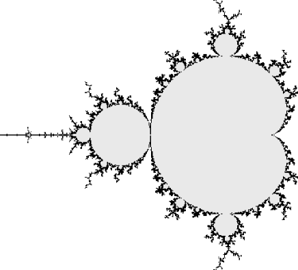
Figure 1. The Mandelbrot set ${\cal M}$

Let $f_{c}$ be a quadratic polynomial with connected Julia set. By Theorem 2.1 the external ray of external argument $0$ lands at a fixed point of $f_{c}$, necessarily repelling or parabolic with multiplier 1, henceforth denoted $\beta_{f_{c}}$. The main hyperbolic component $H_{0}$ is the set of all $c$ for which the other fixed point $\alpha_{f_{c}}$ is attracting; the boundary point $c=1/4$ is hereafter referred to as the root of ${\cal M}$.

The $p/q$-limb $L_{p/q}$ is the connected component of ${\cal M}\setminus H_{0}$ whose boundary contains

$${\operatorname{root}}_{p/q}=\lambda_{H_{0}}^{-1}(e^{2\pi ip/q})$$

and we denote by $H_{p/q}$ the hyperbolic component attached to $H_{0}$ at this point; it is always assumed that $(p,q)=1$. Notice that $L_{0/1}$ is ${\cal M}$ itself. In view of the following, we may refer to $\alpha_{f_{c}}$ as the dividing fixed point.

Lemma 2.11.

For $q\geq 2$, a parameter value $c\in{\cal M}$ lies in $L_{p/q}$ if and only if $\alpha_{f_{c}}$ is the landing point of an external ray with combinatorial rotation number $p/q$.

Consider a polynomial $f_{c}$ with connected Julia set. Let $\zeta_{1}\mapsto\zeta_{2}\mapsto\ldots\mapsto\zeta_{n}=\zeta_{1}$ be a repelling cycle of $f_{c}$, such that each $\zeta_{i}$ is the landing point of at least two external rays. Let $\cal R$ be the collection of all external rays landing at these points, and let $\cal R^{\prime}=-\cal R$ be the symmetric collection. Let us also choose an arbitrary equipotential $E$. Denote by $\Omega$ the component of ${\mathbb{C}}\setminus(\cal R\cup\cal R^{\prime}\cup E)$ containing $0$. This region is bounded by four pieces of external rays and two pieces of $E$. Let $n$ be the period of these rays, $\zeta=\zeta_{i}$ the element of the cycle contained in $\partial\Omega$, and $\Omega^{\prime}\subset\Omega$ the component of $f_{c}^{\circ-n}(\Omega)$ attached to $\zeta$. If $0\in\Omega^{\prime}$ then $f_{c}^{\circ n}:\Omega^{\prime}\to\Omega$ is a branched cover of degree 2.

Following Douady and Hubbard, we say that a polynomial $f_{c}$ is renormalizable if there exists a repelling cycle $\{\zeta_{i}\}$ as above, such that $0\in\Omega^{\prime}$ and $0$ does not escape $\Omega^{\prime}$ under iteration of $f_{c}^{\circ n}$. In this case $f_{c}^{\circ n}|_{\Omega^{\prime}}$ can be extended to a quadratic-like map $f_{c}^{\circ n}:U\to V$ with connected Julia set by a thickening procedure (a version of this procedure is employed in §5). To emphasize the dependence of this construction on the choice of periodic orbit, we shall say that this renormalization of $f_{c}$ is associated to $\zeta$.

Recall that the $\omega$-limit set of a point $z$ under a map $f$ is defined as

$$\omega_{f}(z)=\{w|f^{\circ n_{k}}(z)\to w\mbox{ for some }n_{k}\to\infty\}.$$

When $f=f_{c}$ we simply write $\omega_{c}(z)$ and pay special attention to the $\omega$-limit set of the critical point 0. The following observation will be useful along the way:

Remark 2.12.

For a renormalizable quadratic polynomial $f_{c}$ with $n$ as above,

$$\omega_{c}(0)\subset\displaystyle\bigcup_{i=0}^{n-1}f_{c}^{\circ i}(\overline{\Omega^{\prime}})\cap J(f_{c}).$$

In particular, $\beta_{f_{c}}\not\in\omega_{c}(0)$.

Theorem 2.13 (Douady and Hubbard, [DH2]).

Let $f_{c_{0}}$ be a renormalizable quadratic polynomial with associated periodic point $\zeta$. Then there exists a canonical embedding of the Mandelbrot set ${\cal M}$ onto a subset ${\cal M}^{\prime}\ni c_{0}$ such that every map $f_{c}$ with $c\in{\cal M}^{\prime}\setminus\{\operatorname{one\>point}\}$ is renormalizable with associated repelling periodic point $\zeta_{c}$, where $c\mapsto\zeta_{c}$ is continuous and $\zeta_{c_{0}}=\zeta$.

These subsets ${\cal M}^{\prime}$ are customarily referred to as the small copies of the Mandelbrot set. The inverse homeomorphism $\kappa:{\cal M}^{\prime}\to{\cal M}$ is defined in terms of the straightening map $\chi$:

$${\cal M}^{\prime}\ni c\;\;\mapsto\;\;f_{c}^{\circ n}:U_{c}\to V_{c}\;\;\overset{\chi}{\mapsto}\;\;\kappa(c)\in{\cal M}.$$

The periodic point $\zeta_{c}$ becomes parabolic with multiplier 1 at the excluded parameter value, hereafter referred to as the root of ${\cal M}^{\prime}$. We write ${\cal M}_{p/q}$ for the small copy “growing” from the hyperbolic component $H_{p/q}$, its root being the point root_p/q.

2.4. Cubic polynomials

The connectedness locus, types of hyperbolic components, Per${}_{n}(\lambda)-$curves, real cubic family

We now turn our attention to cubic polynomials. Our presentation follows the detailed discussion in [Mil2].

Observe that every cubic polynomial is affine conjugate to a map of the form

(2.2) $$F_{a,b}(z)=z^{3}-3a^{2}z+b,$$

with critical points $a$ and $-a$. This normal form is unique up to conjugation by $z\mapsto-z$, which interchanges $F_{a,b}$ and $F_{a,-b}$. The pair of complex numbers $A=a^{2}$ and $B=b^{2}$ parameterize the space of cubic polynomials modulo affine conjugacy.

The cubic connectedness locus is the set ${\mathcal{C}}\subset{\mathbb{C}}^{2}$ of all pairs $(A,B)$ for which the corresponding polynomial $F_{a,b}$ has connected Julia set. As in the quadratic case, the connectedness locus is compact and connected with connected complement. These results were obtained by Branner and Hubbard [BH] who showed moreover that this set is cellular, the intersection of a sequence of strictly nested closed discs. On the other hand, Lavaurs [La] proved that ${\mathcal{C}}$ is not locally connected (compare Appendix B).

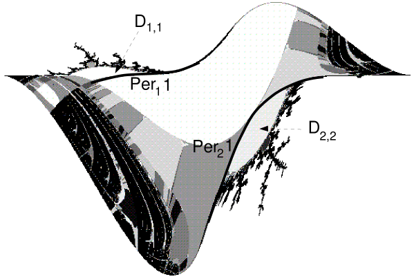
Figure 2. Connectedness locus ${\mathcal{C}}_{{\mathbb{R}}}$ in the real cubic family

Milnor distinguishes four different types of hyperbolic components, according to the behavior of the critical points: adjacent, bitransitive, capture, and disjoint [Mil2]. We are exclusively interested in the last possibility: a component ${\cal H}\subset\overset{\circ}{{\mathcal{C}}}$ is of disjoint type $D_{m,n}$ if $F_{a,b}$ has distinct attracting periodic orbits with periods $m$ and $n$ for every $(a^{2},b^{2})\in{\cal H}$. By definition, the $\operatorname{Per}_{n}(\lambda)-$curve consists of all parameter values for which the cubic polynomial $F_{a,b}$ has a periodic point of period $n$ and multiplier $\lambda$. The geography of $\operatorname{Per}_{1}(0)$ was studied in [Mil3] and [Fa].

Notice that if the coefficients of a cubic polynomial are real then so are the corresponding parameters $A$ and $B$. Thus we may consider the connectedness locus of real cubic maps, the set of pairs $(A,B)\in{\mathbb{R}}^{2}$ such that $J(F_{a,b})$ is connected. This locus ${\mathcal{C}}_{{\mathbb{R}}}$ is also compact, connected and cellular [Mil2]. We refer the reader to Fig. 2 which was generated by a computer program of Milnor. The real slices of various hyperbolic components are rendered in different shades of gray. Certain disjoint type components are indicated, as are the curves $\operatorname{Per}_{1}(1)\cap{\mathcal{C}}_{{\mathbb{R}}}$ and $\operatorname{Per}_{2}(1)\cap{\mathcal{C}}_{{\mathbb{R}}}$.

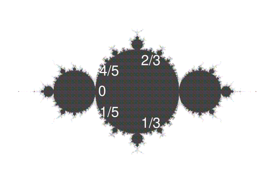
Figure 3. Symmetry locus in the family $P_{A,D}$

To avoid ambiguities arising from the choice of normalization, we will actually work in the family of cubics

$$P_{A,D}=A(w^{3}-3w)+D,\;\;A\neq 0$$

with marked critical points $-1$ and $+1$. The reparametrization

$${\mathbb{C}}^{*}\times{\mathbb{C}}\ni(A,D)\mapsto(A,AD^{2})=(A,B)\in{\mathbb{C}}^{*}\times{\mathbb{C}}$$

is branched over the symmetry locus $B=0$ consisting of normalized cubics which commute with $z\mapsto-z$ (see Fig. 3). In particular,

$${\mathcal{C}}^{\#}=\{(A,D)\subset{\mathbb{C}}^{*}\times{\mathbb{C}}|\;J(P_{A,D})\;\operatorname{is\;connected}\}$$

is a branched double cover of ${\mathcal{C}}\cap({\mathbb{C}}^{*}\times{\mathbb{C}})$. The marking of critical points allows us to label the attracting cycles of maps in disjoint type components ${\cal H}\subset{\mathcal{C}}^{\#}$, and we denote the corresponding multipliers $\lambda^{\pm}_{\cal H}(A,D)$. It is shown in [Mil4] that the maps $\Lambda_{\cal H}:{\cal H}\to{\mathbb{D}}\times{\mathbb{D}}$ given by

$$\Lambda_{\cal H}(A,D)=(\lambda^{-}_{\cal H}(A,D)\,,\lambda^{+}_{\cal H}(A,D))$$

are biholomorphisms. The omitted curve $A=0$, consisting of maps with a single degenerate critical point, is irrelevant to the discussion of disjoint type components.

This useful change of variable has the unfortunate side-effect that the values $(A,D)\in{\mathbb{R}}^{*}\times{\mathbb{R}}$ only account for the first and third quadrants of the real $(A,B)-$plane, the second and fourth quadrants being parameterized by ${\mathbb{R}}^{*}\times i{\mathbb{R}}$. We are therefore unable to furnish a faithful illustration of the entire locus

$${\mathcal{C}}^{\#}_{{\mathbb{R}}}=\{(A,D)|\;(A,AD^{2})\in{\mathcal{C}}_{{\mathbb{R}}}\}.$$

2.5. Tools

Let $f:W^{\prime}\to W$ be a quadratic-like map with connected Julia set, $\zeta$ a repelling fixed point with combinatorial rotation number $p/q$ and associated quotient torus $T_{\zeta}=(D\setminus\{\zeta\})/f^{\circ q}$, where $D$ is a fixed but otherwise arbitrary linearizing neighborhood $D\ni\zeta$. Given $S\subset W\setminus\{\zeta\}$ with $f^{\circ q}(S\cap D)=S\cap f^{\circ q}(D)$, we denote $\hat{S}$ its projection to $T_{\zeta}$; in particular, $\hat{K}_{1}(f),\ldots,\hat{K}_{q}(f)\subset T_{\zeta}$ are the quotients of the various components of $K(f)\setminus\{\zeta\}$. As any two annuli $A_{1}\supset\hat{K}_{i_{1}}(f)$ and $A_{2}\supset\hat{K}_{i_{2}}(f)$ are isotopic we may speak of a distinguished isotopy class of annuli $A\subset T_{\zeta}$, namely $A\sim\hat{K}(f)$ if and only if $A$ is isotopic to an annulus containing some $\hat{K}_{i}(f)$. Moreover, it is easy to see if $A\subset\hat{K}_{i}(f)$ does not separate $T_{\zeta}$ then $A\sim\hat{K}(f)$; it follows then that $\zeta$ is on the boundary of an immediate attracting basin. Consider

$$\underline{\operatorname{mod}}\;\hat{K}_{i}(f)=\sup\{\operatorname{mod}A|\;A\subset\hat{K}_{i}(f)\}$$

and

$$\overline{\operatorname{mod}}\;\hat{K}_{i}(f)=\inf\{\operatorname{mod}A|\;A\supset\hat{K}_{i}(f)\}$$

over annuli $A\sim\hat{K}(f)$. Notice that these quantities are independent of $i$. In view of the following we may simply write ${\operatorname{mod}}\;\hat{K}(f)$:

Lemma 2.14.

In this setting $\underline{\operatorname{mod}}\;\hat{K}_{i}(f)=\overline{\operatorname{mod}}\;\hat{K}_{i}(f)$.

Proof.

It is obvious that $\underline{\operatorname{mod}}\;\hat{K}\leq\overline{\operatorname{mod}}\;\hat{K}$ for $\hat{K}=\hat{K}_{i}(f)$. Conversely, given $R_{n}\searrow R_{\infty}=e^{\overline{\operatorname{mod}}\;K}$ there exist conformal embeddings $h_{n}:{{\mathbb{A}}}_{R_{n}}\to T_{\zeta}$ such that $h_{n}({{\mathbb{A}}}_{R_{n}})\supset\hat{K}_{i}(f)$, where

$${{\mathbb{A}}}_{R}=\{z:1<|z|<R\}.$$

It follows from standard estimates in geometric function theory that the $h_{n}$ form a normal family on ${{\mathbb{A}}}_{R_{\infty}}$; moreover, as all of these embeddings are isotopic, every limit $h_{\infty}=\lim_{k\to\infty}h_{n_{k}}$ is univalent. Clearly, $h_{\infty}({{\mathbb{A}}}_{R_{\infty}})\subset\hat{K}$ and therefore $\overline{\operatorname{mod}}\;\hat{K}\leq\underline{\operatorname{mod}}\;\hat{K}$. ∎

As $\underline{\operatorname{mod}}\;\hat{K}(f)$ is defined in terms of the interior of $K(f)$, we observe:

Remark 2.15.

${\operatorname{mod}}\;\hat{K}(f)={\operatorname{mod}}\;\hat{K}(g)$ at corresponding fixed points of hybrid equivalent quadratic-like maps $f$ and $g$.

Let $f:W^{\prime}\to W$ be a quadratic-like map with connected Julia set, and $\zeta$ a repelling fixed point with combinatorial rotation number $p/q$. An invariant sector with vertex $\zeta$ is a simply connected domain $S\subset W$ bounded by an arc of $\partial W$ and two additional arcs $\gamma_{1}$ and $\gamma_{2}$ with $\gamma_{j}\subset f^{\circ q}(\gamma_{j})$ and a common endpoint at $\zeta$. We write $S=\backslash\gamma_{1},\gamma_{2}/$ for the sector between $\gamma_{1}$ and $\gamma_{2}$ as listed in counterclockwise order. The quotient $\hat{S}\subset T_{\zeta}$ is an open annulus whose modulus will be referred to as the opening modulus $\operatorname{mod}S$ of the sector $S$.

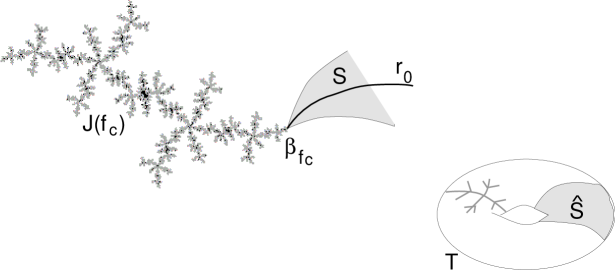
Figure 4. An invariant sector $S_{t}(r_{0})$ with vertex at $\beta_{f_{c}}$

Consider a restriction of a quadratic polynomial $f_{c}$ with a connected Julia set to the domain $W\supset K(f_{c})$ bounded by an equipotential $E_{\rho}$. Invariant sectors for this map may be constructed as follows [BD]: given a ray $r_{\theta}$ landing at a fixed point $\zeta$ with combinatorial rotation number $p/q$, consider

$$S_{t}(r_{\theta})=B_{f_{c}}^{-1}(\{e^{r+2\pi i\gamma}|\;1<r<\rho\;\mbox{ and }\;|\gamma-\theta|<tr\}).$$

Fig. 4 depicts an invariant sector $S=S_{t}(r_{0})$ and its quotient $\hat{S}$.

Lemma 2.16 ([BF], Prop. 4.1).

Given $\rho>1$ there exists $\tau>0$ such that for any $t<\tau$ the domains $S_{t}(r_{2^{i-1}\theta})\subset W$ for $i=1,\ldots,q$ are disjoint invariant sectors.

For the readers convenience let us review the notion of an almost complex structure. Let $\sigma=\{E_{z}\}_{z\in G}$ be a measurable field of ellipses on a planar domain $G$ with the ratio of major to minor axes at the point $z$ denoted by $K(z)$. The complex dilatation is a complex valued function $\mu:G\to{\mathbb{D}}$, where $|\mu(z)|=(K(z)-1)/(K(z)+1)$, and the argument of $\mu(z)$ is twice the argument of the major axis of $E_{z}$. A bounded measurable almost complex structure is a field of ellipses $\sigma$ with $\|\mu\|_{\infty}<1$. The standard almost complex structure $\sigma_{0}$ is a field of circles, thus having identically vanishing complex dilatation.

Given an ellipse field $\sigma$ on $G$ and an almost everywhere differentiable homeomorphism $h:W\to G$ the pullback of $\sigma$ is an ellipse field $h^{*}\sigma$ on $W$ obtained as follows. For almost every $z\in W$, there is a linear tangent map

$$T_{z}h:T_{z}W\to T_{h(z)}G.$$

Let $\sigma=\{E_{\zeta}\subset T_{\zeta}(G)\}_{\zeta\in G}$, then $h^{*}\sigma$ is given by $\{T_{z}h^{-1}(E_{h(z)})\subset T_{z}W\}_{z\in W}$. We note that when the map $h$ is quasiconformal the pullback of the standard structure $\sigma=h^{*}\sigma_{0}$ is a bounded almost complex structure.

The proofs of the following general principles can be found in [LV]:

Theorem 2.17.

Let $h$ be a quasiconformal map such that $h^{*}\sigma_{0}=\sigma_{0}$. Then $h$ is conformal.

Theorem 2.18 (Measurable Riemann Mapping Theorem).

If $\sigma$ is a bounded almost complex structure on a domain $G\subset{\mathbb{C}}$, then there exists a quasiconformal homeomorphism $h:G\to{\mathbb{C}}$, such that

$$\sigma=h^{*}\sigma_{0}.$$

3. Outline of the Results

In the picture of the real cubic connectedness locus (Fig. 2) one observes several shapes reminiscent of the Mandelbrot set (Fig. 1). We quote Milnor ([Mil2]): “… these embedded copies tend to be discontinuously distorted at one particular point, namely the period one saddle node point $c=1/4$, also known as the root of the Mandelbrot set. The phenomenon is particularly evident in the lower right quadrant, which exhibits a very fat copy of the Mandelbrot set with the root point stretched out to cover a substantial segment of the saddle-node curve $\operatorname{Per}_{2}(1)$. $\ldots$ As a result of this stretching, the cubic connectedness locus fails to be locally connected along this curve.”

The original goal of our investigation was to explain the appearance of these distorted copies of the Mandelbrot set embedded in ${\mathcal{C}}_{{\mathbb{R}}}$. This has lead us to the following results:

For $p/q\in{{\mathbb{Q}}}/{{\mathbb{Z}}}$ we consider the set $C_{p/q}\subset{\mathcal{C}}^{\#}$ consisting of cubic polynomials for which $2q$ distinct external rays with combinatorial rotation number $p/q$ land at some fixed point $\zeta$. As there can be at most one such point, the various $C_{p/q}$ are disjoint. Each $C_{p/q}$ is in turn the disjoint union of subsets $C_{p/q,m}$ indexed by an odd integer $1\leq m\leq 2q-1$ specifying how many of these rays are encountered in passing counterclockwise from the critical point $-1$ to the critical point $+1$. In particular, $C_{0}$ consists of those cubics in ${\mathcal{C}}^{\#}$ whose fixed rays $r_{0}$ and $r_{1/2}$ land at the same fixed point.

Theorem 3.1 (Main Theorem).

Given $p/q$ and $m$ as above, there exists a homeomorphic embedding

$$h_{p/q,m}:{\cal M}_{p/q}\setminus\{{\operatorname{root}}_{p/q}\}\,\times\,{\cal M}_{p/q}\setminus\{{\operatorname{root}}_{p/q}\}\,\longrightarrow\,C_{p/q,m}\,$$

mapping the product of hyperbolic components $H_{p/q}\times H_{p/q}$ onto a component ${\cal H}_{p/q,m}$ of type $D_{q,q}$.

We note that ${\cal H}_{p/q,m}$ is the unique $D_{q,q}$ component contained in $C_{p/q,m}$ as will follow from Theorem 5.6. The restriction of $h_{p/q,m}$ to $H_{p/q}\times H_{p/q}$ is easily expressed in terms of the multiplier maps defined in §2:

$$h_{p/q,m}(\rho,\tilde{\rho})=\Lambda_{{\cal H}_{p/q,m}}^{-1}(\,\lambda_{H_{p/q}}(\rho),\lambda_{H_{p/q}}(\tilde{\rho})\,).$$

Discontinuity of $h_{p/q,m}$ at the corner point $(1,1)$ is a special case of a phenomenon studied by one of the authors:

Theorem 3.2.

[Ep] Each algebraic homeomorphism

$$\Lambda_{{\cal H}_{p/q,m}}:{\cal H}_{p/q,m}\to{\mathbb{D}}\times{\mathbb{D}}$$

extends to a continuous surjection $\bar{{\cal H}}_{p/q,m}\to\bar{{\mathbb{D}}}\times\bar{{\mathbb{D}}}$. The fiber over $(1,1)$ is the union of two closed discs whose boundaries are real-algebraic curves with a single point in common, and all other fibers are points.

The following reasonable conjecture appears to be inaccessible by purely quasiconformal techniques:

Conjecture 3.1.

Each $h_{p/q,m}$ extends to a continuous embedding

$${\cal M}_{p/q}\times{\cal M}_{p/q}\,\setminus\,\{({\operatorname{root}}_{p/q},{\operatorname{root}}_{p/q})\}\,\longrightarrow\,C_{p/q,m}\,.$$

We draw additional conclusions from the natural symmetries of our construction. The central disk in Fig. 3 is parameterized by the eigenvalue $-3A$ of the attracting fixed point at $0$; this region corresponds to symmetric cubics whose Julia sets are quasicircles. Each value $A=-\frac{1}{3}e^{2\pi ip/q}$ yields a map with a parabolic fixed point at 0. These parameters are evidently the roots of small embedded copies of ${\cal M}$, and our results confirm this observation for odd-denominator rationals. More specifically, it will follow that the latter copies are the images of $h_{0}\circ\Delta$ and $h_{p/q,q}\circ\Delta$ for odd $q>1$, where

$${\mathbb{C}}\ni c\overset{\Delta}{\mapsto}(c,c)\in{\mathbb{C}}^{2}$$

is the diagonal embedding. As $P^{\circ 2}_{A,0}$ and $P^{\circ 2}_{-A,0}$ are conjugate by $z\mapsto-z$, our construction also accounts for the copies with $q\equiv 2$ (mod $4)$. Every map in the symmetry locus is semiconjugate, via the quotient determined by the involution, to a cubic polynomial with a fixed critical value. Such maps were studied by Branner and Douady [BD] who effectively prove that the entire limb attached at the parameter value $A=-1/3$ is a homeomorphic copy of the limb $L_{1/2}\subset{\cal M}$; it can be shown by a variant of the pullback argument in §5 that the image of $h_{0}\circ\Delta$ corresponds to the small copy ${\cal M}_{1/2}\subset L_{1/2}$.

Similar considerations applied to the antidiagonal embedding yield results for the real connectedness locus. In view of the fact that real polynomials commute with complex conjugation, ${\mathcal{C}}^{\#}_{{\mathbb{R}}}\cap C_{p/q}=\emptyset$ unless $p/q\equiv-p/q\;\mbox{(mod 1)}$, and it therefore suffices to consider the real slices of $C_{1/2}$ and $C_{0}$.

Theorem 3.3.

There exist homeomorphic embeddings

$$\Psi_{1/2,1}:{\cal M}_{1/2}\setminus\{{\operatorname{root}}_{1/2}\}\to{\mathcal{C}}^{\#}_{{\mathbb{R}}}\cap C_{1/2,1}$$

$$\Psi_{1/2,3}:{\cal M}_{1/2}\setminus\{{\operatorname{root}}_{1/2}\}\to{\mathcal{C}}^{\#}_{{\mathbb{R}}}\cap C_{1/2,3}$$

and

$$\Psi_{0}:{\cal M}\setminus\{{\operatorname{root}}\}\to{\mathcal{C}}^{\#}_{{\mathbb{R}}}\cap C_{0}.$$

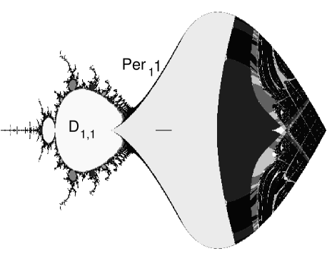
Figure 9. The view of the comb on the $D_{1,1}$ component in $(A,b)$ parametrization

It follows from recent work of Buff [Bu] that these maps are compatible with the standard embeddings in the plane (see the discussion in §5.4). Their projections in ${\mathcal{C}}_{{\mathbb{R}}}$ are indicated in Fig. 2. Notice that the two images of ${\cal M}_{1/2}\setminus\{{\operatorname{root}}_{1/2}\}$ have been identified while the image of ${\cal M}\setminus\{{\operatorname{root}}\}$ has been folded in half. The latter defect is overcome through passage to the $(A,\sqrt{B})$-plane, at the cost of both copies of $M_{1/2}\setminus\{{\operatorname{root}}_{1/2}\}$; we thank J. Milnor for enabling us to include Fig. 9 where the comb on the $D_{1,1}$ component is better resolved. The existence of this comb is verified with the aid of techniques developed by Lavaurs [La].

Theorem 3.4.

The real cubic connectedness locus is not locally connected.

The remainder of this paper is structured as follows. In §4 we construct cubic polynomials by means of quasiconformal surgery on pairs of quadratics. The issues of uniqueness and continuity are addressed in §5 through the use of the renormalization operators ${\operatorname{R}}$ and ${Ya}$ defined for birenormalizable cubics; together they essentially invert the surgery. We show that ${\operatorname{R}}\times{Ya}$ is a homeomorphism and then complete the proofs of Theorems 3.1 and 3.3 in §5.4. The measurable dynamics of birenormalizable maps is discussed in §6. In Appendix A we comment further on the discontinuity described in Theorem 3.2, and we conclude by proving Theorem 3.4 in Appendix B.

It is worth noting that quasiconformal surgery is only employed in the proof of surjectivity for ${\operatorname{R}}\times{Ya}$. More generally, we might associate a pair of renormalization operators to any disjoint type hyperbolic component ${\cal H}\subset{\mathcal{C}}^{\#}$ in the hope of finding an embedded product of Mandelbrot sets “growing” from ${\cal H}$, but we are unable to adapt our surgery construction to this broader setting. Part II of this paper will present a different approach to proving surjectivity of birenormalization, culminating in a more general version of Theorem 3.1.

4. Intertwining surgery

4.1. History

The intertwining construction was described in the 1990 Conformal Dynamics Problem List [Bi2]: “Let $P_{1}$ be a monic polynomial with connected Julia set having a repelling fixed point $x_{0}$ which has ray landing on it with rotation number $p/q$. Look at a cycle of $q$ rays which are the forward images of the first. Cut along these rays and get $q$ disjoint wedges. Now let $P_{2}$ be a monic polynomial with a ray of the same rotation number landing on a repelling periodic point of some period dividing $q$ (such as $1$ or $q$). Slit this dynamical plane along the same rays making holes for the wedges. Fill the holes in by the corresponding wedges above making a new sphere. The new map is given by $P_{1}$ and $P_{2}$, except on a neighborhood of the inverse images of the cut rays where it will have to be adjusted to make it continuous.”

4.2. Construction of a cubic polynomial

Fix $p/q$ written in lowest terms and an odd integer $m=2k+1$ between 1 and $2q-1$. Our aim is to construct a map

$$h_{p/q,m}:{\cal M}_{p/q}\setminus\{{\operatorname{root}}_{p/q}\}\,\times\,{\cal M}_{p/q}\setminus\{{\operatorname{root}}_{p/q}\}\longrightarrow C_{p/q,m}.$$

Fixing parameter values $c$ and $\tilde{c}$ in ${\cal M}_{p/q}\setminus\{{\operatorname{root}}_{p/q}\}$, consider quadratic-like maps $f:W^{\prime}\to W$ and $\tilde{f}:\tilde{W}^{\prime}\to\tilde{W}$ hybrid equivalent to $f_{c}$ and $\tilde{f}_{c}$ respectively, the choice of the hybrid equivalences to be made below. In what follows we will identify $W$ and $\tilde{W}$ to obtain a new surface. The reader is invited to follow the construction in the particular case $p/q=1/2$ with $m=3$, as illustrated in Fig. 5.

We lose no generality by assuming that $0$ is the critical point for both $f$ and $\tilde{f}$. Let $\zeta$ be the unique repelling fixed point of $f$ with combinatorial rotation number $p/q$, that is $\zeta=\beta_{f}$ for $p/q=0$ and $\zeta=\alpha_{f}$ otherwise, and $S_{i}\equiv\backslash l_{i},r_{i}/,\;i=0,\ldots,q$ in $W\setminus K(f)$ a cycle of disjoint invariant sectors with vertex $\zeta$, indexed in counterclockwise order so that the critical point $0$ lies in the complementary region between $S_{q-1}$ and $S_{0}$. We similarly specify $\tilde{\zeta}$ and a cycle of invariant sectors $\tilde{S}_{i}$ for $\tilde{f}$. Let

$$\phi:\bigcup_{i=1}^{q}l_{i}\cup r_{i}\to\bigcup_{i=1}^{q}\tilde{l}_{i}\cup\tilde{r}_{i}$$

sending $l_{i}$ to $\tilde{r}_{i+q-k}$ and $r_{i}$ to $\tilde{l}_{i+q-k-1}$, where $k=(m-1)/2$ and indices are understood modulo $q$, be any smooth conjugacy,

$$\phi(f(z))={\tilde{f}}(\phi(z)).$$

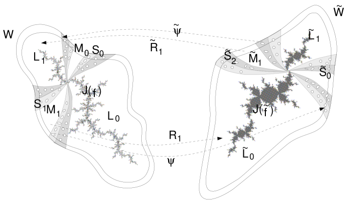
Figure 5. Superimposing the regions $W$ and $\tilde{W}$

The sector $S_{i}$ should now correspond to the component of $K(\tilde{f})\setminus\{\tilde{\zeta}\}$ containing $\tilde{f}^{\circ i+q-k}(0)$. An informal rule known as Shishikura’s Principle warns against altering the conformal structure on regions of uncontrolled recurrence, and we will therefore employ invariant sectors $M_{i}\subset S_{i}\subset N_{i}\subset W\setminus K(f)$ and $\tilde{M}_{i}\subset\tilde{S}_{i}\subset\tilde{M}_{i}\subset\tilde{W}\setminus K(\tilde{f})$ to be determined below. For $i=0,\ldots,q$ denote $L_{i}$ the component of $W\setminus\bigcup_{j=1}^{q}N_{j}$ containing $f^{\circ i}(0)$, and $\tilde{L}_{i}$ the corresponding component of $\tilde{W}\setminus\bigcup_{j=1}^{q}\tilde{N}_{j}$. Let

$$R_{i}:M_{i}\to\tilde{L}_{i+q-k}$$

be the conformal homeomorphism sending $\partial M_{i}\cap W$ to $\partial\tilde{L}_{i+q-k}\cap\tilde{W}$ so that $\zeta$ maps to $\tilde{\zeta}$, and

$$\tilde{R}_{i}:\tilde{M}_{i}\to L_{i-q+k+1}$$

the conformal homeomorphism sending $\partial\tilde{M}_{i}\cap\tilde{W}$ to $\partial L_{i-q+k+1}\cap W$ so that $\tilde{\zeta}$ maps to $\zeta$. These Riemann maps extend continuously to the sector boundaries, and it remains to fill in the gaps:

Proposition 4.1 (Quasiconformal interpolation).

For any pair $f_{c}$ and $f_{\tilde{c}}$ as above the hybrid equivalent quadratic-like maps $f$ and $\tilde{f}$ and the invariant sectors

$$N_{i}\supset S_{i}\supset M_{i}\;\mbox{ and }\;\tilde{N}_{i}\supset\tilde{S}_{i}\supset\tilde{M}_{i}$$

may be chosen so that there exist quasiconformal maps

$$\psi:\bigcup_{i=1}^{q}(S_{i}\setminus M_{i})\to\bigcup_{i=1}^{q}(\tilde{N}_{i}\setminus\tilde{S}_{i})$$

$$\tilde{\psi}:\bigcup_{i=1}^{q}(\tilde{S}_{i}\setminus\tilde{M}_{i})\to\bigcup_{i=1}^{q}(N_{i}\setminus S_{i})$$

with

$$\psi|_{\partial M_{i}}=R_{i}|_{\partial M_{i}}\;\mbox{ and }\;\psi|_{\partial S_{i}}=\phi|_{\partial S_{i}}$$

$$\tilde{\psi}|_{\partial\tilde{M}_{i}}=\tilde{R}_{i}|_{\partial\tilde{M}_{i}}\;\mbox{ and }\;\tilde{\psi}|_{\partial\tilde{S}_{i}}=\tilde{\phi}|_{\partial\tilde{S}_{i}}.$$

Let us complete the construction assuming the truth of Proposition 4.1. We choose sectors $N_{i}$, $M_{i}$, $\tilde{N}_{i}$, $\tilde{M}_{i}$, and maps $\psi$, $\tilde{\psi}$ as specified above. These identifications turn $W\sqcup\tilde{W}$ into a new manifold with a natural quasiconformal atlas. Consider the almost complex structure $\sigma$ on $W$, given by $\psi^{*}\sigma_{0}$ on $\bigcup_{i=1}^{q}S_{i}\setminus M_{i}$ and by $\sigma_{0}$ elsewhere; similarly, let $\tilde{\sigma}$ be the almost complex structure on $\tilde{W}$ given by $\tilde{\psi}^{*}\sigma_{0}$ on $\bigcup_{i=1}^{q}\tilde{S}_{i}\setminus\tilde{M}_{i}$, and $\sigma_{0}$ elsewhere. In view of Theorem 2.18 there exist quasiconformal homeomorphisms $h:W\to X$ and $\tilde{h}:\tilde{W}\to\tilde{X}$ such that $\sigma=h^{*}\sigma_{0}$ and $\tilde{\sigma}=\tilde{h}^{*}\sigma_{0}$. The domains $X$ and $\tilde{X}$ give coordinate neighborhoods, and the maps $\psi\circ h^{-1}$, $R_{i}\circ h^{-1}$, $\tilde{\psi}\circ\tilde{h}^{-1}$, and $\tilde{R}_{i}\circ\tilde{h}^{-1}$ yield an atlas of a Riemann surface with the conformal type of a punctured disc. We obtain a conformal disc $\Delta$ by replacing the puncture with a point $\star$. Setting

$$\Delta^{\prime}=h(W^{\prime}\setminus\bigcup_{i=1}^{q}S_{i})\cup\tilde{h}(\tilde{W}^{\prime}\setminus\bigcup_{i=1}^{q}\tilde{S}_{i})\cup\{\star\},$$

we define a new map $F:\Delta^{\prime}\to\Delta$ by

$$F(z)=\left\{\begin{array}[]{lll}h(f(h^{-1}(z)))&\mbox{for}&z\in h(W^{\prime}\setminus\bigcup_{i=1}^{q}S_{i}),\\ \tilde{h}(\tilde{f}(\tilde{h}^{-1}(z)))&\mbox{for}&z\in\tilde{h}(\tilde{W}^{\prime}\setminus\bigcup_{i=1}^{q}\tilde{S}_{i}),\\ \star&\mbox{for}&z\in\{\star,-\zeta,-\tilde{\zeta}\}.\end{array}\right.$$

It is easily verified that $F$ is a three-fold branched covering with critical points $h(0)$ and $\tilde{h}(0)$, and analytic except on the preimage of

$${\cal S}=\bigcup_{i=1}^{q}h(S_{i}\setminus M_{i})\cup\tilde{h}(\tilde{S}_{i}\setminus\tilde{M}_{i}).$$

Recalling that the sectors $S_{i}$ and $\tilde{S}_{i}$ are invariant and disjoint, we consider the following almost complex structure on $\Delta$:

$$\left\{\begin{array}[]{ll}\hat{\sigma}=(F^{\circ n})^{*}\sigma_{0}&\mbox{on }F^{\circ-n}({\cal S})\\ \hat{\sigma}=\sigma_{0}&\mbox{elsewhere }.\end{array}\right.$$

By construction, the complex dilatation of $\hat{\sigma}$ has the same bound as that of $F^{*}\sigma_{0}$, and moreover

$$F^{*}\hat{\sigma}=\hat{\sigma}.$$

It follows from Theorem 2.18 that there is a quasiconformal homeomorphism $\varphi:\Delta\to V\subset{\mathbb{C}}$ with $\hat{\sigma}=\varphi^{*}\sigma_{0}$. Setting $U=\varphi(\Delta^{\prime})$, we obtain a cubic-like map

$$G=\varphi\circ F\circ\varphi^{-1}:U\to V.$$

In view of Theorem 2.6 there is a unique hybrid equivalent cubic polynomial $P_{A,D}$ whose critical points $-1$ and $+1$ correspond to the critical point of $f$ and $\tilde{f}$ respectively. The construction yields extensions of the natural embeddings

$$\pi:K(f_{c})\to K(P_{A,D})\;\mbox{ and }\;\tilde{\pi}:K(f_{\tilde{c}})\to K(P_{A,D})$$

to neighborhoods of the filled Julia sets.

Remark 4.2.

By construction, the projections $\pi$ and $\tilde{\pi}$ are conformal on the respective filled Julia sets:

$$\bar{\partial}\pi=0\mbox{ a.e. on }K(f_{c})\;\mbox{ and }\;\bar{\partial}{\tilde{\pi}}=0\mbox{ a.e. on }K(f_{\tilde{c}}).$$

We write $P_{A,D}\approx f_{c}{\underset{p/q,m}{\curlyvee}}f_{\tilde{c}}$ for any cubic polynomial so obtained. It is not yet clear that this correspondence is well-defined, let alone continuous. These issues will be addressed in §5.

4.3. Quasiconformal interpolation

Proof of Proposition 4.1:
Note first that were it not for the condition of quasiconformality, the existence of the interpolating maps $\psi$ and $\tilde{\psi}$ would follow without any additional argument. Any smooth interpolations are quasiconformal away from the points of $\zeta$ and $\tilde{\zeta}$, the issue is the compatibility of the the local behaviour of $\phi$ at $\zeta$ with that of $R_{i}$ and $\tilde{R}_{i}$.

Lemma 4.3.

Given any $c\in{\cal M}_{p/q}\setminus\{{\operatorname{root}}_{p/q}\}$ and $\upsilon>0$, there exists a quadratic-like map $f$ which is hybrid equivalent to $f_{c}$ and admits disjoint invariant sectors $S_{i}$ as above with ${\operatorname{mod}}\;S_{i}>\upsilon$.

Proof.

We begin by fixing a quadratic-like restriction $f_{c}:G^{\prime}\to G$ between equipotentially bounded regions, and apply Lemma 2.16 to obtain a cycle of disjoint invariant sectors $S_{t}(r_{i})\subset G$. Let $\varphi$ be a quasiconformal homeomorphism from the annulus $\hat{S}_{t}(r_{0})\subset T_{\zeta}$ to some standard annulus ${{\mathbb{A}}}_{\rho}$ with $\rho>e^{\upsilon}$. The almost complex structure $\sigma=\varphi^{*}\sigma_{0}$ on $\hat{S}_{t}(r_{0})$ lifts to an almost complex structure on the sector $S_{t}(r_{0})$. We extend this structure by pullback to the various $S_{t}(r_{i})$ and their preimages, and extend by $\sigma_{0}$ elsewhere, to obtain an invariant almost complex structure $\bar{\sigma}$ on $G$. In view of Theorem 2.18 there exists a quasiconformal homeomorphism $\varphi:G\to\varphi(G)\subset{{\mathbb{C}}}$ with $\bar{\sigma}=\varphi^{*}\sigma_{0}$, giving a hybrid equivalence between $f_{c}$ and the quadratic-like map

$$f=\varphi\circ f_{c}\circ\varphi^{-1}:\varphi(G^{\prime})\to\varphi(G).$$

It follows from Theorem 2.17 that ${\operatorname{mod}}\;S_{i}=\upsilon$ where

$$S_{i}=\varphi(S_{t}(r_{i})).$$

∎

Given $c,\tilde{c}\in{\cal M}_{p/q}\setminus\{{\operatorname{root}}_{p/q}\}$, we apply Lemma 4.3 to $f_{c}$ and $f_{\tilde{c}}$ to obtain hybrid equivalent quadratic-like maps $f$ and $\tilde{f}$ admitting invariant sectors $S_{i}$ and $\tilde{S}_{i}$ with

$${\operatorname{mod}}\;S_{i}>{\operatorname{mod}}\;\hat{K}(f_{\tilde{c}})\;\mbox{ and }\;{\operatorname{mod}}\;\tilde{S}_{i}>{\operatorname{mod}}\;\hat{K}(f_{c}).$$

In view of Remark 2.15 we may then choose disjoint invariant sectors $N_{i}\supset S_{i}$ and $\tilde{N}_{i}\supset\tilde{S}_{i}$ so that

$${\operatorname{mod}}\;S_{i}>{\operatorname{mod}}\;\tilde{L}_{j}\;\mbox{ and }\;{\operatorname{mod}}\;\tilde{S}_{i}>{\operatorname{mod}}\;L_{j}$$

for the complementary invariant sectors $L_{j}$,$\tilde{L}_{j}$ as above. Finally, we choose $M_{i}\subset S_{i}$ and $\tilde{M}_{i}\subset\tilde{S}_{i}$ with

$${\operatorname{mod}}\;M_{i}={\operatorname{mod}}\;\tilde{L}_{j}\;\mbox{ and }\;{\operatorname{mod}}\;\tilde{M}_{i}={\operatorname{mod}}\;L_{j}.$$

We now exploit the following observation of [BD]; see [Bi1, Lemmas 6.4, 6.5] for a detailed exposition.

Lemma 4.4.

With this choice of maps and invariant sectors there exist desired quasiconformal interpolations

$$\psi:\bigcup_{i=1}^{q}(S_{i}\setminus M_{i})\to\bigcup_{i=1}^{q}(\tilde{N}_{i}\setminus\tilde{S}_{i})$$

$$\tilde{\psi}:\bigcup_{i=1}^{q}(\tilde{S}_{i}\setminus\tilde{M}_{i})\to\bigcup_{i=1}^{q}(N_{i}\setminus S_{i})$$

with

$$\psi|_{\partial M_{i}}=R_{i}|_{\partial M_{i}}\;\mbox{ and }\;\psi|_{\partial S_{i}}=\phi|_{\partial S_{i}}$$

$$\tilde{\psi}|_{\partial\tilde{M}_{i}}=\tilde{R}_{i}|_{\partial\tilde{M}_{i}}\;\mbox{ and }\;\tilde{\psi}|_{\partial\tilde{S}_{i}}=\tilde{\phi}|_{\partial\tilde{S}_{i}}.$$

5. Renormalization

5.1. Birenormalizable cubics

Throughout this section we will work with fixed values of $p/q$ and $m$ as specified above. Here we describe the construction which will provide the inverse to the map $h_{p/q,m}$.

We start with a cubic polynomial $P=P_{A,D}$ with $(A,D)\in C_{p/q,m}$. Let $\zeta$ be the landing point of the periodic rays with rotation number $p/q$, and denote $K_{\pm 1}$ the connected components of $K(P)\setminus\{\zeta\}$ containing the critical points $\pm 1$. Below we determine quadratic-like restrictions of $P$ which domains contain the appropriate critical points. To fix the ideas, we illustrate this thickening procedure for left renormalizations only.

Let $r_{\theta_{1}}$ and $r_{\theta_{2}}$ be the two periodic external rays landing at $\zeta$ which separate $K_{-1}$ from the other rays landing there; without loss of generality, $0\leq\theta_{2}<\theta_{1}<2\pi$ so that the rays landing at $K_{-1}$ have angles in $[\theta_{2},\theta_{1}]$. Choose a neighborhood $U\ni\zeta$ corresponding to a round disc in the local linearizing coordinate. Fix an equipotential $E$ and a small $\epsilon>0$, and consider the segments of the rays $r_{\theta_{1}+\epsilon}$ and $r_{\theta_{2}-\epsilon}$ connecting the boundary of $U$ to $E$. Let $\Omega\supset K_{-1}$ be the region bounded by these two ray segments and the subtended arcs of $E$ and $\partial U$, and consider the component $\Omega^{\prime}$ of $P^{\circ-q}(\Omega)$ with $\Omega^{\prime}\subset\Omega$. In view of the fact that $\zeta$ is repelling, $\bar{\Omega}^{\prime}\subset\Omega$ provided that $\epsilon$ is sufficiently small. Thus,

$$P^{\circ q}:\Omega^{\prime}\to\Omega$$

is a quadratic-like map which filled Julia set will be denoted $K_{\operatorname{R}}$. This set is connected if and only if $\{P^{\circ nq}(-1)\}_{n=0}^{\infty}\subset K_{-1}$, in which case we refer to the unique hybrid conjugate quadratic polynomial $f_{c}$ as the left renormalization ${\operatorname{R}}(P)$ and call $P$ renormalizable to the left.

Fig. 6 illustrates this construction for a cubic polynomial in $C_{0}$. Notice that $\zeta$ becomes the $\beta-$fixed point of the new quadratic polynomial. The polynomial $P$ is renormalizable to the right if $\{P^{\circ nq}(+1)\}_{n=0}^{\infty}\subset K_{+1}$, and the set $K_{{Ya}}$ and the right renormalization ${Ya}(P)$ are correspondingly defined. It follows from general considerations discussed in [McM1] that the left and right renormalizations do not depend on the choice of thickened domains.

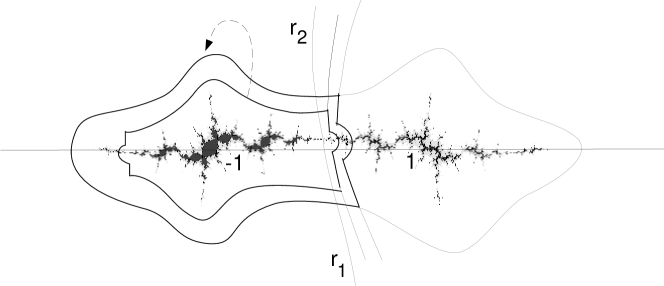
Figure 6. Construction of the left renormalization for a cubic in $C_{0}$

A cubic polynomial $P$ is said to be birenormalizable if it is renormalizable on both left and right, in which case

(5.1) $$\omega_{P}(-1)\cap\omega_{P}(+1)\subset K_{{\operatorname{R}}}\cap K_{{Ya}}=\{\zeta\}$$

and we set

$$\check{K}(P)=\bigcup_{i=0}^{\infty}P^{-\circ i}(K_{\operatorname{R}}\cup K_{{Ya}}).$$

The following is an easy consequence of Kiwi’s Separation Theorem 2.4 and the standard classification of Fatou components:

Lemma 5.1.

Let $P$ be a birenormalizable cubic polynomial. Then $\check{K}(P)$ is dense in $K(P)$, and every periodic orbit in $K(P)\setminus\check{K}(P)$ is repelling.

We denote $B_{p/q,m}$ the set of birenormalizable cubics in $C_{p/q,m}$, writing

$${\operatorname{R}}\times{Ya}:B_{p/q,m}\to({\cal M}\setminus\{{\operatorname{root}}\})\times(M\setminus\{{\operatorname{root}}\})$$

for the map $(A,D)\mapsto(c,\tilde{c})$ where $f_{c}={\operatorname{R}}(P_{A,D})$ and $f_{\tilde{c}}={Ya}(P_{A,D})$. In view of Lemma 2.3 the thickening construction may be performed so that the domains of the left and right quadratic-like restrictions vary continuously for $(A,D)\in B_{p/q,m}$. Applying Theorem 2.7 we obtain:

Proposition 5.2.

${\operatorname{R}}\times{Ya}:B_{p/q,m}\to({\cal M}\setminus\{{\operatorname{root}}\})\times({\cal M}\setminus\{{\operatorname{root}}\})$ is continuous.

The significance of intertwining rests in the following:

Proposition 5.3.

${\operatorname{R}}\times{Ya}:B_{p/q,m}\to({\cal M}\setminus\{{\operatorname{root}}\})\times({\cal M}\setminus\{{\operatorname{root}}\})$ is surjective.

Proof.

Fixing $b,\tilde{b}\in{\cal M}\setminus\{{\operatorname{root}}\}$, let $c=\kappa_{p/q}^{-1}(b)$ and $\tilde{c}=\kappa_{p/q}^{-1}(b)$ where

$$\kappa_{p/q}:{\cal M}_{p/q}\to{\cal M}$$

is the homeomorphism described in §2.3. We saw above that

$$f_{c}{\underset{p/q,m}{\curlyvee}}f_{\tilde{c}}\approx P$$

for some cubic polynomial $P=P_{A,D}$, and we show here that ${\operatorname{R}}\times{Ya}(A,D)=(b,\tilde{b})$; more precisely, we prove that ${\operatorname{R}}(P)=f_{b}$, the argument for right renormalization being completely parallel.

Let $K(f_{c})\subset W{\overset{\pi}{\rightarrow}}{\mathbb{C}}$ be as in §4. The standard thickening construction yields a quadratic-like restriction $f_{c}^{\circ q}:G^{\prime}\to G$ with connected filled Julia set $K\subset G\subset W$; as $f_{c}^{\circ q}|_{G^{\prime}}\underset{\operatorname{hb}}{\sim}f_{b}$ it suffices to show that this quadratic-like map is hybrid equivalent to $P^{\circ q}|_{\Omega^{\prime}}$. By construction, $\pi$ is a quasiconformal map conjugating $f_{c}^{\circ q}|_{K}$ to $P^{\circ q}|_{K_{{\operatorname{R}}}}$ and $\bar{\partial}\pi(z)=0$ for almost every $z\in K$. Let $\varphi_{0}:G\to\Omega$ be a quasiconformal homeomorphism with

$$\varphi_{0}\circ f_{c}^{\circ q}|_{\partial G^{\prime}}=P^{\circ q}\circ\varphi_{0}|_{\partial\Omega^{\prime}}$$

which agrees with $\pi$ on a small neighborhood of $K$. As $\varphi_{0}$ maps the critical value of $f_{c}^{\circ q}|_{\partial G^{\prime}}$ to the critical value of $P^{\circ q}|_{\partial\Omega^{\prime}}$ there is a unique lift $\varphi_{1}:G^{\prime}\to\Omega^{\prime}$ such that

$$\begin{CD}G^{\prime}@>{\varphi_{1}}>{}>\Omega^{\prime}\\ @V{f_{c}^{\circ q}}V{}V@V{P^{\circ q}}V{}V\\ G@>{q_{0}}>{}>\Omega\end{CD}$$

commutes and $\varphi_{1}|_{\partial G^{\prime}}=\varphi_{0}|_{\partial G^{\prime}}$. Setting $\varphi_{1}(z)=\varphi_{0}(z)$ for $z\in\Omega\setminus\Omega^{\prime}$, we obtain a quasiconformal homeomorphism $\varphi_{1}:G\to\Omega$ with the same dilatation bound as $\varphi_{0}$; moreover, $\varphi_{1}|_{K}=\pi|_{K}$. Iteration of this procedure yields a a sequence of quasiconformal homeomorphisms $\varphi_{n}:G\to\Omega$ with uniformly bounded dilatation. The $\varphi_{n}$ stabilize pointwise on $G$, so there is a limiting quasiconformal homeomorphism $\varphi:G\to\Omega$. By construction,

$$\varphi\circ f_{c}^{\circ q}|_{G^{\prime}}=P^{\circ q}\circ\varphi|_{\Omega}$$

and furthermore $\varphi|_{K}=\pi|_{K}$; it follows from Bers’ Lemma 2.8 that $\varphi$ is a hybrid equivalence. ∎

5.2. Properness

Here we deduce the properness of birenormalization from Kiwi’s Separation Theorem 2.4.

Proposition 5.4.

${\operatorname{R}}\times{Ya}:B_{p/q,m}\to({\cal M}\setminus\{{\operatorname{root}}\})\times({\cal M}\setminus\{{\operatorname{root}}\})$ is proper.

In view of the compactness of the connectedness loci, it suffices to prove that if $(A_{k},D_{k})\in B_{p/q,m}$ with

$$(A_{k},D_{k})\to(A_{\infty},D_{\infty})\in{\mathcal{C}}^{\#}\;\;\mbox{ and }\;\;{\operatorname{R}}\times{Ya}(A_{k},D_{k})\to(c_{\infty},\tilde{c}_{\infty})\in{\cal M}\times{\cal M}$$

then $(A_{\infty},D_{\infty})\in B_{p/q,m}$ if and only if $c_{\infty}\neq{\operatorname{root}}\neq\tilde{c}_{\infty}$. We require an auxiliary lemma and some further notation. Let $\zeta_{k}$ be the unique repelling fixed point of $P_{k}=P_{A_{k},D_{k}}$ where $2q$ external rays land, and let $\zeta_{k}^{-}$ and $\zeta_{k}^{+}$ be the points of period $q$ which renormalize to $\alpha_{f_{c_{k}}}$ and $\alpha_{f_{\tilde{c}_{k}}}$. We write $\mu_{k}$ and $\mu^{\pm}_{k}$ for the multipliers of $\zeta_{k}$ and $\zeta^{\pm}_{k}$, and $\lambda_{k}^{\pm}$ for the multipliers of the corresponding $\alpha$-fixed points. Passing to a subsequence if necessary, we may assume without loss of generality that the $\zeta_{k}$ converge to a fixed point $\zeta_{\infty}$ of $P_{\infty}=P_{A_{\infty},D_{\infty}}$ with multiplier $\mu_{\infty}$, and the $\zeta_{k}^{\pm}$ converge to periodic points $\zeta^{\pm}_{\infty}$ with multipliers $\mu^{\pm}_{\infty}$.

Lemma 5.5.

In this setting, if $c_{\infty}\neq{\operatorname{root}}\neq\tilde{c}_{\infty}$ then $\zeta^{-}_{\infty}$, $\zeta_{\infty}$ and $\zeta^{+}_{\infty}$ belong to disjoint orbits. Moreover, the fixed point $\zeta_{\infty}$ is repelling.

Proof.

It follows from the Implicit Function Theorem that these orbits are distinct unless one of $\zeta^{\pm}_{\infty}$ is parabolic with multiplier 1. Without loss of generality $\mu_{\infty}^{-}=1$, and we may further assume that either $|\mu^{-}_{k}|\leq 1$ for every $k$ or $|\mu^{-}_{k}|>1$ for every $k$. In the first case, $\lambda^{-}_{k}=\mu^{-}_{k}$ by Remark 2.5, and $\lambda^{-}_{k}\to 1$ implies $c={\operatorname{root}}$. In the second case, it similarly follows that $|\lambda^{-}_{k}|>1$ for every $k$; in view of Yoccoz Inequality, $c_{k}\in L_{p_{k}/q_{k}}$ where $p_{k}/q_{k}\to 0$, whence $\lambda^{-}_{k}\to 1$ and again $c={\operatorname{root}}$.

Because $\zeta_{\infty}^{-}$, $\zeta_{\infty}$ and $\zeta^{\pm}_{\infty}$ lie in distinct orbits, it follows from Theorem 2.4 that at least one of these points is repelling. Suppose first that $\zeta^{-}_{\infty}$ is repelling, and let $\gamma^{-}_{k}\in K(P_{k})$ be the points which renormalize to $-\alpha_{f_{c_{k}}}\in K(f_{c_{k}})$. Then $\gamma^{-}_{k}\to\gamma^{-}_{\infty}$ where $P_{\infty}(\gamma^{-}_{\infty})=\zeta^{-}_{\infty}$, and the rays landing at $\gamma^{-}_{\infty}$ separate $\zeta_{\infty}$ from the critical point $-1$. Similarly, if $\zeta^{+}_{\infty}$ is repelling then the rays landing at the corresponding point $\gamma^{+}_{\infty}$ separate $\zeta_{\infty}$ from $+1$. Applying Theorem 2.4 once again, we conclude that $\zeta_{\infty}$ is repelling. ∎

Continuing with the proof of Proposition 5.4, we observe by Lemma 2.3 that $\zeta_{\infty}$ is the common landing point of the same two cycles of rays with rotation number $p/q$. The thickening procedure yields a pair of quadratic-like restrictions

$$P_{\infty}^{\circ q}:\Omega_{\infty}^{\prime}\to\Omega_{\infty}\;\;\operatorname{and}\;\;P_{\infty}^{\circ q}:\tilde{\Omega}_{\infty}^{\prime}\to\tilde{\Omega}_{\infty},$$

and we may arrange for $\Omega^{\prime}_{\infty}$ and $\tilde{\Omega}^{\prime}_{\infty}$ to be the limits of thickened domains $\Omega^{\prime}_{k}$ and $\tilde{\Omega}^{\prime}_{k}$ for the quadratic-like restrictions of $P^{\circ q}_{k}$. As $P_{k}^{\circ qn}(-1)\in\Omega^{\prime}_{k}$ and $P_{k}^{\circ qn}(+1)\in\tilde{\Omega}^{\prime}_{k}$, it follows that $P_{\infty}^{\circ qn}(-1)\in\Omega^{\prime}_{\infty}$ and $P_{\infty}^{\circ qn}(+1)\in\tilde{\Omega}^{\prime}_{\infty}$. Thus, $P_{\infty}$ is birenormalizable, that is, $(A_{\infty},D_{\infty})\in B_{p/q,m}$. $\;\;\Box$

5.3. Injectivity

The time has come to show that the intertwining operations

$$(f,\tilde{f})\mapsto f{\underset{p/q,m}{\curlyvee}}\tilde{f}$$

are well-defined:

Proposition 5.6.

${\operatorname{R}}\times{Ya}:B_{p/q,m}\to({\cal M}\setminus\{{\operatorname{root}}\})\times({\cal M}\setminus\{{\operatorname{root}}\})$ is injective.

The relevant pullback argument is formalized as:

Lemma 5.7.

Let $P=P_{A,D}$ and $Q=P_{\tilde{A},\tilde{D}}$ where $(A,D),\,(\tilde{A},\tilde{D})\in B_{p/q,m}$. If

$${\operatorname{R}}\times{Ya}(A,D)={\operatorname{R}}\times{Ya}(\tilde{A},\tilde{D})$$

then there exists a quasiconformal homeomorphism $\varphi:{\mathbb{C}}\to{\mathbb{C}}$ conjugating $P$ to $Q$ with $\bar{\partial}\varphi=0$ almost everywhere on $\check{K}(P)$

Proof.

We begin by once again restricting $P$ and $Q$ to domains $D\supset K(P)$ and $\tilde{D}\supset K(Q)$ bounded by equipotentials. Our first goal is the construction of a quasiconformal homeomorphism $\varphi_{0}$ which is illustrated in Fig. 7 for $p/q=1/2$ and $m=3$. Let $r_{1},\ldots,r_{2q}$ be the rays landing at $\zeta$, enumerated in counterclockwise order so that the connected component $K_{-1}\ni-1$ of $K(P)\setminus\{\zeta\}$ lies between $r_{1}$ and $r_{2}$; the component $K_{+1}\ni+1$ then lies between $r_{m+1}$ and $r_{m+2}$. We label the remaining components of $K(P)\setminus\{\zeta\}$ as $K_{\pm 1}^{1},\ldots,K_{\pm 1}^{q-1}$, so that $K_{\pm 1}^{i}\ni P^{\circ i}(\pm 1)$. The corresponding objects associated to $Q$ are similarly denoted with an added tilde.

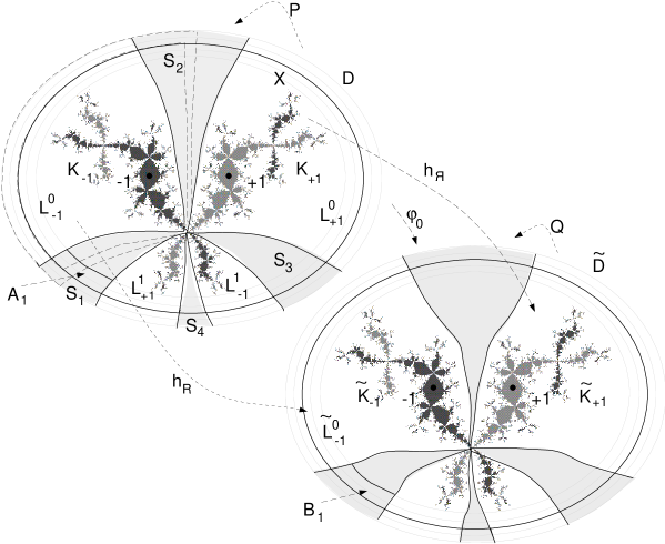
Figure 7. Construction of the map $\varphi_{0}$ in the case $p/q=1/2$ with $m=3$

It will be convenient to introduce further notation. Let $S_{i}\subset D$ be disjoint invariant sectors centered at $r_{i}$, and let $L^{i}_{\pm 1}$ be the component of $P^{\circ-q}(D)\setminus(\bigcup_{j=1}^{2q}S_{j})$ containing $K_{\pm 1}^{i}$. The thickening procedure yields left and right quadratic-like restrictions

$$P^{\circ q}:\Omega^{\prime}_{{\operatorname{R}}}\to\Omega_{{\operatorname{R}}}\;\;\operatorname{and}\;\;P^{\circ q}:\Omega^{\prime}_{{Ya}}\to\Omega_{{Ya}}$$

and

$$Q^{\circ q}:\tilde{\Omega}^{\prime}_{{\operatorname{R}}}\to\tilde{\Omega}_{{\operatorname{R}}}\;\;\operatorname{and}\;\;Q^{\circ q}:\tilde{\Omega}^{\prime}_{{Ya}}\to\tilde{\Omega}_{{Ya}}.$$

By assumption, there exist hybrid equivalences $h_{{\operatorname{R}}}$ between $P^{\circ q}|_{\Omega^{\prime}_{{\operatorname{R}}}}$ and $Q^{\circ q}|_{\tilde{\Omega}^{\prime}_{{\operatorname{R}}}}$, and $h_{{Ya}}$ between $P^{\circ q}|_{\Omega^{\prime}_{{Ya}}}$ and $Q^{\circ q}|_{\tilde{\Omega}^{\prime}_{{Ya}}}$. We now replace the domains $D$ and $\tilde{D}$ by $X=P^{\circ-q}(D)$ and $\tilde{X}=Q^{\circ-q}(\tilde{D})$. We define the map $\varphi_{0}$ on $\bigcup_{i=0}^{q-1}L_{\pm 1}^{i}\subset X$ as

$$\varphi_{0}(z)=\left\{\begin{array}[]{lll}h_{{\operatorname{R}}}(z)&\mbox{ for }&z\in L_{-1}^{0},\\ h_{{Ya}}(z)&\mbox{ for }&z\in L_{+1}^{0},\\ Q^{\circ-(q-i)}\circ h_{{\operatorname{R}}}\circ P^{\circ q-i}(z)&\mbox{ for }&z\in L_{-1}^{i}\mbox{ with }i>0,\\ Q^{\circ-(q-i)}\circ h_{{Ya}}\circ P^{\circ q-i}(z)&\mbox{ for }&z\in L_{+1}^{i}\mbox{ with }i>0.\\ \end{array}\right.$$

where by $Q^{\circ-(q-i)}$ we understand the univalent branch mapping $\tilde{K}_{\pm 1}$ to $\tilde{K}_{\pm 1}^{i}$.

Let $A_{i}$ be the strip of $X\setminus P^{\circ-q}(X)$ contained in $S_{i}$, and $B_{i}$ its counterpart in $\tilde{X}\setminus Q^{\circ-q}(\tilde{X})$. We smoothly extend $\varphi_{0}$ to map $A_{i}\to B_{i}$ in agreement with the previously specified values of $\varphi_{0}$ on $\partial(L_{-1}^{i}\cup L_{+1}^{i})$ and $\varphi_{0}\circ P^{\circ q}=Q^{\circ q}\circ\varphi_{0}$ on the inner boundary of $A_{i}$. We now extend $\varphi_{0}$ to the entire sector $S_{i}\cap X$ by setting $\varphi_{0}(z)=Q^{\circ-nq}\circ\varphi_{0}\circ P^{\circ nq}(z)$ when $P^{\circ nq}(z)\in A_{i}$.

The quasiconformal homeomorphism $\varphi_{0}:X\to\tilde{X}$ so defined conjugates $P$ to $Q$ on the set $\bigcup_{i=0}^{q-1}P^{\circ i}(K_{{\operatorname{R}}}\cup K_{{Ya}})$, with $\bar{\partial}\varphi_{0}=0$ almost everywhere on this set, sending each $P^{\circ i}(K_{{\operatorname{R}}})$ to $Q^{\circ i}(\tilde{K}_{{\operatorname{R}}})$ and each $P^{\circ i}(K_{{Ya}})$ to $Q^{\circ i}(\tilde{K}_{{Ya}})$. We further extend $\varphi_{0}$ to a quasiconformal homeomorphism from $Y=P(X)$ to $\tilde{Y}=Q(\tilde{X})$ so that

$$\varphi_{0}\circ P|_{\partial X}=Q\circ\varphi_{0}|_{\partial X}.$$

As $\varphi_{0}$ is a conjugacy between postcritical sets, there is a unique lift $\varphi_{1}:X\to\tilde{X}$ agreeing with $\varphi_{0}$ on $\bigcup_{i=0}^{q-1}P^{\circ i}(K_{{\operatorname{R}}}\cup K_{{Ya}})$ such that the following diagram commutes:

$$\begin{CD}X@>{\varphi_{1}}>{}>\tilde{X}\\ @V{P}V{}V@V{Q}V{}V\\ Y@>{\varphi_{0}}>{}>\tilde{Y}\end{CD}$$

As in the proof of Proposition 5.3, we set $\varphi_{1}(z)=\varphi_{0}(z)$ for $z$ in the annulus $Y\setminus X$, and iterate the lifting procedure to obtain a sequence of quasiconformal maps $\varphi_{n}$ with uniformly bounded dilatation. In view of the density of $\check{K}(P)$ in $K(P)$, the limiting map $\varphi:Y\to\tilde{Y}$ conjugates $P$ to $Q$. As $\varphi_{n}$ stabilizes pointwise on $\check{K}(P)$ with $\varphi|_{K_{{\operatorname{R}}}}=h_{{\operatorname{R}}}$ and $\varphi|_{K_{{Ya}}}=h_{{Ya}}$ by construction, it follows from Bers’ Lemma 2.8 that $\bar{\partial}\varphi=0$ almost everywhere on $\check{K}(P)$. ∎

To conclude the proof of Proposition 5.6, we show that the conjugacy just obtained is actually a hybrid equivalence: that any measurable invariant linefield on $K(P)\setminus\check{K}(P)$ has support in a set of Lebesgue measure 0. In view of Lemma 5.7, it follows from the standard considerations of parameter dependence in the Measurable Riemann Mapping Theorem (2.18) that ${\cal F}=({\operatorname{R}}\times{Ya})^{-1}(A,D)$ is the injective complex-analytic image of a polydisc ${{\mathbb{D}}}^{k}$ for some $k\in\{0,1,2\}$; see [MSS] and [McS]. On the other hand, $\cal F$ is compact by Proposition 5.4, whence $k=0$ and $\cal F$ is a single point. $\;\;\Box$

5.4. Conclusions

Setting

$$h_{p/q,m}(c,\tilde{c})=({\operatorname{R}}\times{Ya})^{-1}(\kappa_{p/q}(c),\kappa_{p/q}(\tilde{c}))$$

so that $h_{p/q,m}(c,\tilde{c})=(A,D)$ if and only if $P_{A,D}=f_{c}{\underset{p/q,m}{\curlyvee}}f_{\tilde{c}}$ we obtain the embeddings

$$h_{p/q,m}:({\cal M}_{p/q}\setminus\{{\operatorname{root}}_{p/q}\})\times({\cal M}_{p/q}\setminus\{{\operatorname{root}}_{p/q}\})\longrightarrow B_{p/q,m}\subset C_{p/q,m}$$

whose existence was asserted in Theorem 3.1. As observed in §3, if $P=P_{A,D}$ is birenormalizable and $(A,D)\in{\mathcal{C}}^{\#}_{{\mathbb{R}}}$ then $p/q=0$ or $1/2$. It follows by symmetry that ${\operatorname{R}}\times{Ya}(A,D)=(c,\bar{c})$ for some $c\in{\mathbb{C}}$; conversely, if ${\operatorname{R}}\times{Ya}(A,D)=(c,\bar{c})$ then $(A,D)\in{\mathcal{C}}^{\#}_{{\mathbb{R}}}$. Writing $\bar{\Delta}$ for the antidiagonal embedding ${\mathbb{C}}\ni c\mapsto(c,\bar{c})\in{{\mathbb{C}}}^{2}$, we define

$$\Psi_{1/2,1}=h_{1/2,1}\circ\bar{\Delta}:{\cal M}_{1/2}\setminus\{{\operatorname{root}}_{1/2}\}\to{\mathcal{C}}^{\#}_{{\mathbb{R}}}\cap C_{1/2,1}$$

$$\Psi_{1/2,3}=h_{1/2,3}\circ\bar{\Delta}:{\cal M}_{1/2}\setminus\{{\operatorname{root}}_{1/2}\}\to{\mathcal{C}}^{\#}_{{\mathbb{R}}}\cap C_{1/2,3}$$

and

$$\Psi_{0}=h_{0}\circ\bar{\Delta}:{\cal M}\setminus\{{\operatorname{root}}\}\to{\mathcal{C}}^{\#}_{{\mathbb{R}}}\cap C_{0}.$$

These are the embeddings whose existence was asserted in Theorem 3.3. Compatibility with the standard planar embeddings is a consequence of the following recent result of Buff [Bu]:

Theorem 5.8.

Let $K_{1}$ and $K_{2}$ be compact, connected, cellular sets in the plane, and $\varphi:K_{1}\to K_{2}$ a homeomorphism. If $\varphi$ admits a continuous extension to an open neighborhood of $K_{1}$ such that points outside $K_{1}$ map to points outside $K_{2}$, then $\varphi$ extends to a homeomorphism between open neighborhoods of $K_{1}$ and $K_{2}$.

Let us sketch the argument for the map $\Psi_{0}$. It is easily verified from the explicit expressions in [Mil2, p. 22] that for each $\mu\in{{\mathbb{C}}}\setminus\{1\}$ there is a unique pair $(A,B)\in{\mathbb{R}}^{2}$ such that the corresponding polynomial in the normal form (2.2) has a pair of complex conjugate fixed points with multipliers $\mu$ and $\bar{\mu}$, the remaining fixed point having eigenvalue

$$\nu=1+\frac{|\mu-1|^{2}}{2\operatorname{Re}(\mu-1)}.$$

We may continuously label these multipliers as $\mu(A,D)$, $\bar{\mu}(A,D)$ and $\nu(A,D)$ for parameter values $(A,D)\in{\mathbb{R}}\times i{\mathbb{R}}$ in a neighborhood of $\Psi_{0}({\cal M}\setminus\{{\operatorname{root}}\})$; in particular, $(A,D)\mapsto\mu(A,D)$ is a homeomorphism on such a neighborhood. It follows from Yoccoz Inequality (2.1) that $\nu(A,D)>1$, and therefore $\mu(A,D)\not\in[1,\infty)$, for $(A,D)$ in $\Psi_{0}({\cal M}\setminus\{{\operatorname{root}}\})$. Similarly, $\mu(\Psi_{0}(c))\to 1$ as $c\to{\operatorname{root}}$, and thus $c\mapsto\mu(\Psi_{0}(c))$ extends to a embedding

$$\Upsilon:{\cal M}\to{\mathbb{C}}\setminus(1,\infty)$$

which clearly commutes with complex conjugation.

We claim that $\Upsilon^{-1}:\Upsilon({\cal M})\to{\cal M}$ admits a continuous extension meeting the condition of Theorem 5.8. The idea is to allow renormalizations with disconnected Julia sets. Recalling Lemma 2.3, we note that the rays $r_{0}$ and $r_{1/2}$ continue to land at the same fixed point for $(A,D)$ in a neighborhood of $\Psi_{0}({\cal M}\setminus\{{\operatorname{root}}\})$. As before, we may construct left and right quadratic-like restrictions with continuously varying domains $\Omega^{\prime}_{A,D}$. It is emphasized in Douady and Hubbard’s original presentation [DH2] that straightening, while no longer canonical for maps with disconnected Julia set, may still be continuously defined: it is only necessary to begin with continuously varying quasiconformal homeomorphisms from the fundamental annuli $\Omega_{A,D}\setminus\Omega^{\prime}_{A,D}$ to the standard annulus. We thereby obtain a continuous extension to a neighborhood of $\Upsilon({\cal M}\setminus\{{\operatorname{root}}\})$; it is easily arranged that this extension commutes with complex conjugation, so that it is trivial to obtain a further extension to an open set containing the point $1$.

6. Measure of the Residual Julia Set

Recall that for a birenormalizable polynomial $P$,

$$\check{K}(P)=\bigcup_{i=0}^{\infty}P^{-\circ i}(K_{\operatorname{R}}\cup K_{{Ya}}).$$

Here we synthesize various arguments of Lyubich to show that the residual Julia set $K(P)\setminus\check{K}({P})$ has Lebesgue measure 0, provided that neither renormalization lies in the closure of the main hyperbolic component of ${\cal M}$. Subject to this restriction, we arrive at an alternative proof that the conjugacy constructed in Lemma 5.7 is a hybrid equivalence. We formalize the statement as follows:

Theorem 6.1.

Let $P$ be a birenormalizable cubic polynomial. If all three fixed points are repelling then $K(P)\setminus\check{K}(P)$ has Lebesgue measure 0.

The main technical tool for us will be the celebrated Yoccoz puzzle construction which we briefly recall below:

Yoccoz puzzle and recurrence. Let $f=f_{c}$ be a quadratic polynomial with connected Julia set, and $G\supset K(f)$ be a domain bounded by some fixed equipotential curve. As observed in Lemma 2.11, if $c\in L_{p/q}$ for some $q\geq 2$ then $\alpha_{f}$ is the landing point of a cycle of $q$ external rays. The Yoccoz puzzle of depth zero consists of the $q$ pieces $Y^{0}_{1},$ $Y^{0}_{2},\ldots,Y^{0}_{q}$ obtained by cutting $G$ along these rays, and the puzzle pieces of depth $n>0$ are the connected components $Y^{n}_{i}$ of the various $f^{\circ-n}(Y^{0}_{i})$. Each point $z\in K(f)\setminus f^{\circ-n}(\alpha)$ lies in a unique depth $n$ puzzle piece $Y^{n}(z)$. A nonrenormalizable polynomial $f$ has a reluctantly recurrent critical point if there exists $k\geq 0$ and a sequence of depths $n_{i}\to\infty$ such that the restriction $f^{\circ n_{i}-k}:Y^{n_{i}}(0)\to Y^{k}(f^{\circ n_{i}-k}(0))$ has degree $2$. Note that, somewhat abusing the notation, we allow maps with non-recurrent critical point in this definition. In the complementary case of persistently recurrent critical point Lyubich has shown the following:

Lemma 6.2.

[Lyu2, p. 6] If the critical point of a non-renormalizable quadratic polynomial $f_{c}$ is persistently recurrent then $f_{c}|_{\omega_{c}(0)}$ is topologically minimal, that is all orbits are dense in $\omega_{c}(0)$. In particular, $\beta_{f_{c}}\not\in\omega_{c}(0)$.

The puzzle construction is easily adapted to a cubic map $P=P_{A,D}$ which has a connected Julia set with empty interior and every periodic orbit repelling. The depth zero puzzle pieces $W^{0}_{i}$ are now obtained by cutting an equipotentially bounded domain $G\supset J(P)$ along every ray which lands at some fixed point, and the pieces of depth $n$ are the connected components of the various $P^{\circ-n}(W^{0}_{i})$. Each point $z\in J(P)\setminus P^{-\circ n}(\{\text{fixed points}\})$ lies in a unique depth $n$ puzzle piece $W^{n}(z)$.

By analogy with the quadratic case, we say that the critical point $\pm 1$ of the cubic polynomial $P=P_{A,D}$ is reluctantly recurrent if there exist $k\geq 0$, $N>0$ and a sequence of depths $n_{i}\rightarrow\infty$ such that $P^{\circ n_{i}-k}|_{W^{n_{i}}(\pm 1)}$ is a map of degree $N$. We readily observe that if $P$ is birenormalizable and one of its renormalizations has a reluctantly recurrent critical point then the corresponding critical point of $P$ is reluctantly recurrent. Indeed in this case the restriction $P^{\circ n-k}|_{W^{n}(1)}$ has the same degree as the map ${\operatorname{R}}(P)^{\circ n-k}$ on the quadratic puzzle piece $Y^{n}(0)$, and similarly for the other renormalization.

Yarrington [Yar] has shown that if both critical points of $P$ are reluctantly recurrent then $J(P)$ is locally connected; in particular nested sequences of puzzle pieces shrink to points in this case:

(6.1) $$\bigcap_{n=0}^{\infty}W^{n}(z)=\{z\}$$

for every $z\in J(P)\setminus\{\text{prefixed points}\}$ ([Yar, Theorem 3.5.7]).

Relative ergodicity. The proof of Theorem 6.1 is based on the following general principle of Lyubich:

Theorem 6.3 ([Lyu1]).

Let $g$ be a rational map with $J(g)\neq\hat{{\mathbb{C}}}$. Then

$$\omega_{g}(z)\subset\bigcup_{\gamma\in\Gamma}\omega_{g}(\gamma)$$

for almost every $z\in J(g)$, where $\Gamma$ is the set of all critical points.

We divide the argument into two cases depending on the recurrence properties of the renormalizations of $P$.

Assume first that $\omega_{P}(-1)\cap\omega_{P}(+1)=\emptyset$. It follows from Theorem 6.3 that for almost every $z\in J(P)$ $\omega_{P}(z)$ lies in the disjoint union $\omega_{P}(-1)\cup\omega_{P}(+1)$. Without loss of generality $\omega_{P}(z)\subset\omega_{P}(-1)$, so there is a subsequence $P^{\circ nq+\ell}(z)$ such that every accumulation point lies in $K_{{\operatorname{R}}}$. In particular, $P^{\circ nq+\ell}(z)\in\Omega^{\prime}$ for sufficiently large $n$, where $\Omega^{\prime}$ is the domain of the left quadratic-like restriction of $P^{\circ q}$. Thus, $P^{\circ nq+\ell}(z)\in K_{{\operatorname{R}}}$ for large enough $n$, and therefore $z\in\bigcup_{i=0}^{\infty}P^{\circ-i}(K_{{\operatorname{R}}})\subset\check{K}(P)$.

In the other case, recall from (5.1) that $\omega_{P}(-1)\cap\omega_{P}(+1)=\{\zeta\}$. Combining Remark 2.12 and Lemma 6.2, we see that both ${\operatorname{R}}(P)$ and ${Ya}(P)$ are nonrenormalizable quadratics with reluctantly recurrent critical points. We conclude the argument by showing that under these conditions the Lebesgue measure of the Julia set of $P$ is zero:

Lemma 6.4.

Let $P=P_{A,D}$ be a birenormalizable cubic with all three fixed points repelling. If both its renormalizations ${\operatorname{R}}(P)$ and ${Ya}(P)$ are nonrenormalizable quadratic maps with reluctantly recurrent critical points, then the Julia set of $P$ has Lebesgue measure zero.

Proof.

We adapt Lyubich’s argument [Lyu2] for the quadratic case. As both critical points of $P$ are reluctantly recurrent, there exist $k$ and arbitrary large $s$ and $t$ such that $P^{\circ s}|_{W^{s+k}(-1)}$ and $P^{\circ t}|_{W^{t+k}(+1)}$ are maps of degree 2. By Theorem 6.3 for a full measure set of $z\in J(P)$ there exists $n$ such that $P^{\circ n}(z)$ lies in $W^{s+k}(-1)\cup W^{t+k}(+1)$ for any $s$ and $t$. Fixing $t$, $s$ and $z$ consider the least such $n$. Without loss of generality, $P^{\circ n}(z)\in W^{s+k}(-1)$ and we obtain a chain of univalent branches of $P^{-1}$

$$W^{s+k}(-1)=X_{0}\leftarrow X_{-1}\leftarrow\ldots\leftarrow X_{-n}\ni z$$

by pulling this piece back along the orbit of $z$.

Fix a puzzle-piece $W_{i}^{k}$ of depth $k$. As the boundary of $W^{k}_{i}$ consists of preimages of external rays landing at the fixed points of $P$ and equipotential curves it follows from Koebe $1/4$ theorem that there exist $\delta_{i}$ and $\delta_{i}^{\prime}$ such that for any $u\in W^{k}_{i}$ with $\operatorname{dist}(\partial W^{k}_{i},u)<\delta_{i}$ some neighborhood $U\subset W^{k}_{i}$ around $u$ is univalently mapped by an iterate $P^{\circ j}$ to a disk $D_{\delta^{\prime}_{i}}(P^{\circ j}(u))$ of radius $\delta_{i}^{\prime}$ centered at $P^{\circ j}(u)$. Denote by $\delta$ the minumum of various $\delta_{i}$, $\delta_{i}^{\prime}$ and set $u=P^{\circ s+n}(z)\in P^{\circ s}({W^{s+k}(-1)})=W^{k}$. By the above, there exists a neighborhood $U\ni u$ in $W^{k}$ and an iterate $P^{\circ j}$ univalently mapping $U$ to $D_{\delta}(P^{\circ j}(u))$.

Assume first that $P^{\circ s}(-1)$ does not belong to $U$, or $|P^{\circ s+j}(-1)-P^{\circ j}(u)|>\delta/100$. The density of the Julia set in a disk of radius $\delta/200$ is bounded away from $1$. Consider the univalent pullback $T_{0}=D_{\delta/200}(P^{\circ j}(u)),T_{-1},\ldots,T_{-s-n-j}$ along the orbit $z\mapsto P(z)\mapsto\ldots\mapsto P^{\circ s+n+j}(z)\in T_{0}$. By the Koebe distortion theorem, the density of $J(P)$ in $T_{-s-n-j}$ is also bounded away from $1$. By the estimate (6.1), the disks $T_{-s-n-j}$ shrink to the point $z$ as $s$ grows and therefore $z$ is not a point of density for the set $J(P)$.

Consider now the case when $P^{\circ s}(-1)\in U$, and $|P^{\circ s+j}(-1)-P^{\circ j}(u)|<\delta/100$. Then we can find a disk $D_{1}$ centered at $P(-1)$, such that $P^{\circ s+j-1}(D_{1})$ is contained between $D_{\delta/10}(P^{\circ j}(u))$ and $D_{\delta/2}(P^{\circ j}(u))$. By Koebe distortion theorem, the density of $J(P)$ in the disk $D_{1}$ is bounded away from $1$. Consider the preimage $D_{0}$ of $D_{1}$ centered around $-1$ and contained in $W^{n+s}(-1)$. The density of the Julia set in $D_{0}$ is again bounded away from $1$, and as in the previous case we conclude that $z$ is not a point of density. Thus the set of density points of $J(P)$ has measure zero, and by Lebesgue density theorem so does $J(P)$. ∎

Appendix A Discontinuity at the corner point

The systematic exclusion of root points is not merely an artifact of our reliance on quasiconformal surgery. It is conceivable that more powerful techniques might someday prove existence and uniqueness of intertwinings $f_{c}{\underset{p/q,m}{\curlyvee}}f_{\tilde{c}}$ for any pair $(c,\tilde{c})\in{\cal M}_{p/q}\times{\cal M}_{p/q}$. Indeed, $f_{c}|_{J(f_{c})}$ for any $c\in H_{p/q}$ is canonically topologically conjugate to $f_{\hat{c}}|_{J(f_{\hat{c}})}$ where $\hat{c}={\operatorname{root}}_{p/q}$, and on these grounds we have put forth Conjecture 3.1. On the other hand, we assert in Theorem 3.2 that such a extension of $h_{p/q,m}$ is necessarily discontinuous at the corner point $({\operatorname{root}}_{p/q},{\operatorname{root}}_{p/q})$. This is an instance of a phenomenon investigated by one of the authors. It is shown in [Ep] that any disjoint type component consisting of maps with adjacent attracting basins must suffer such a discontinuity; for $c,\tilde{c}\in H_{p/q}$ the basins of $f_{c}{\underset{p/q.m}{\curlyvee}}f_{\tilde{c}}$ are adjacent by construction. Here we simply summarize the relevant considerations.

Let $g$ be an analytic map fixing $\zeta\in{\mathbb{C}}$. The holomorphic index of $g$ at $\zeta$ is the residue

$$\eta=\frac{1}{2\pi i}\int_{\gamma}\frac{dz}{z-g(z)}$$

where $\gamma$ is a loop enclosing $\zeta$ but no other other fixed point. It is easily checked that this quantity is conformally invariant; in fact,

$$\eta=\frac{1}{1-\lambda}$$

so long as the multiplier $\lambda=g^{\prime}(\zeta)$ is not equal to 1.

An elementary computation yields

$$\eta_{a}=\frac{1}{2\pi i}\int_{\gamma}\frac{dz}{-az^{2}-z^{3}}=\frac{1}{a^{2}}$$

for the holomorphic index of $Q_{a}(z)=z+az^{2}+z^{3}$ at the parabolic fixed point $0$. In the terminology of [Ep], such a fixed point is described as parabolic-attracting, parabolic-indifferent or parabolic-repelling depending on whether $\operatorname{Re}\eta$ is greater than, equal to, or less than 1. The first of these alternatives applies when $|a^{2}-\frac{1}{2}|<\frac{1}{2}$. The corresponding region in the $a-$plane is bounded by a lemniscate shaped like the symbol $\infty$; its position in the cubic connectedness locus is depicted in Fig. 8, which in view of the 4-dimensionality of $D_{1,1}$ is merely schematic. The intersection of the component boundary with $\operatorname{Per}_{1}(1)$ consists of the closure of this lemniscate (shaded in dark gray, and contained in the light gray region where both critical points lie in the parabolic basin), and a similar locus (the large lobes of the medium gray region) parameterizing maps whose other fixed point is attracting or indifferent; the latter might be described as intertwinings $f_{c}{\underset{0}{\curlyvee}}f_{\tilde{c}}$ for $c\in H_{0}$ and $\tilde{c}={\operatorname{root}}$. These pieces intersect at the parameter value $a=0$ where the parabolic fixed point becomes degenerate.

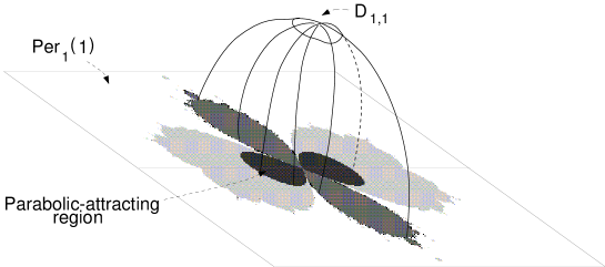
Figure 8. The unique component of type $D_{1,1}$ and its impression on $\operatorname{Per}_{1}(1)$

The crux of the matter is the following elementary observation (compare with [Mil1, Problem 9-1]):

Lemma A.1.

Let $\eta\in{\mathbb{C}}$. Then $\,\operatorname{Re}\eta\geq 1$ if and only if there exist continuous paths $\lambda,\tilde{\lambda}:[0,1)\to{\mathbb{D}}$ with endpoints $\lambda(1)=1=\tilde{\lambda}(1)$ such that

$$\eta=\lim_{t\to 1}\;\frac{1}{1-\lambda(t)}+\frac{1}{1-\tilde{\lambda}(t)}.$$

Complex conjugate paths may be chosen when $\eta$ is real.

Similar considerations apply to $h_{p/q,m}(H_{p/q}\times H_{p/q})$. For odd denominator $p/q$ and $A_{p/q}=-\frac{1}{3}e^{2\pi ip/q}$, it is easy to see that $P_{A_{p/q},0}$ is the unique normalized cubic polynomial with a degenerate parabolic fixed point of multiplier $e^{2\pi ip/q}$; thus

$$\lim_{c\rightarrow{\operatorname{root}}_{p/q}}h_{p/q,q}(c,c)\to(A_{p/q},0)$$

as is evident in Fig. 3.

Appendix B Non local-connectivity of the real connectedness locus

Here we employ a simplified version of an argument of Lavaurs [La] to conclude that the real cubic connectedness locus is not locally connected along an interval in the boundary of $\Psi_{0}({\cal M}\setminus\{{\operatorname{root}}\})$. The existence of comb-like structures in $\Psi_{1/2,i}({\cal M}_{1/2}\setminus\{{\operatorname{root}}_{1/2}\})$ is similarly demonstrated; see also Nakane and Schleicher’s proof of non local-connectivity for the tricorn [NS].

We begin with a brief review of the theory of parabolic bifurcations, as applied in particular to real cubic polynomials. The reader is referred to [Do] for a more comprehensive exposition; supporting technical details may be found in [Sh]. Recall that the fixed point at 0 is parabolic with multiplier 1 for every map in the family

$$Q_{a}(z)=z+az^{2}+z^{3}.$$

Lemma B.1 (Fatou coordinates).

For $a\neq 0$ there exist topological discs $U^{\cal A}_{a}$ and $U^{\cal R}_{a}$ whose union is a punctured neighborhood of the parabolic fixed point, such that

$$Q_{a}(\bar{U}^{\cal A}_{a})\subset U^{\cal A}_{a}\cup\{0\} \bigcap_{k=0}^{\infty}Q_{a}^{\circ k}(\bar{U}^{\cal A}_{a})=\{0\},$$ and

$$Q_{a}^{-1}(\bar{U}^{\cal R}_{a})\subset U^{\cal R}_{a}\cup\{0\} \bigcap_{k=0}^{\infty}Q_{a}^{\circ-k}(\bar{U}^{\cal R}_{a})=\{0\}.$$ and

Moreover, there exist injective analytic maps

$$\Phi^{\cal A}_{a}:U^{\cal A}_{a}\to{\mathbb{C}}\;\;\operatorname{and}\;\;\Phi^{\cal R}_{a}:U^{\cal R}_{a}\to{\mathbb{C}},$$

unique up to post-composition by translations, such that

$$\Phi^{\cal A}_{a}(Q_{a}(z))=\Phi^{\cal A}_{a}(z)+1\;\;\operatorname{and}\;\;\Phi^{\cal R}_{a}(Q_{a}(z))=\Phi^{\cal R}_{a}(z)+1.$$

The quotients $C^{\cal A}_{a}=U^{\cal A}_{a}/Q_{a}$ and $C^{\cal R}_{a}=U^{\cal R}_{a}/Q_{a}$ are therefore Riemann surfaces conformally equivalent to the cylinder ${\mathbb{C}}/{\mathbb{Z}}$.

The quotients $C^{\cal A}_{a}$ and $C^{\cal R}_{a}$ are customarily referred to as the Écalle-Voronin cylinders associated to the map $Q_{a}$; we will find useful to regard these as Riemann spheres with distinguished points $\pm$ filling in the punctures. Every point in the parabolic basin

$${\cal B}_{a}=\{z\in{\mathbb{C}}|\;Q_{a}^{\circ n}(z)\neq 0\mbox{ for }n\geq 0\mbox{ and }Q_{a}^{\circ n}(z)\to 0\}$$

eventually lands in $U^{\cal A}_{a}$, and the return map from $U^{\cal R}_{a}\cap{\cal B}_{a}$ to $U^{\cal A}_{a}$ descends to a well-defined analytic transformation

$${\cal E}_{a}:{\cal W}_{a}\to C^{\cal A}_{a}$$

where ${\cal W}_{a}$ is the image of ${\cal B}_{a}$ on $C^{\cal R}_{a}$. It is easy to see that the ends of $C^{\cal R}_{a}$ belong to different components of ${\cal W}_{a}$. The choice of a conformal transit isomorphism

$$\Theta:C^{\cal A}_{a}\to C^{\cal R}_{a}$$

respecting these ends determines an analytic dynamical system

$${\cal F}_{a:\Theta}=\Theta\circ{\cal E}_{a}:{\cal W}_{a}\to C^{\cal R}_{a}$$

with fixed points at $\pm$. The product of the corresponding eigenvalues $\varrho^{\pm}_{a:\Theta}$ is clearly independent of $\Theta$, indeed

$$\varrho^{+}_{a:\Theta}\cdot\varrho^{-}_{a:\Theta}=e^{-4\pi^{2}(\eta_{a}-1)}=e^{-4\pi^{2}(\frac{1}{a^{2}}-1)}.$$

For $a\in{\mathbb{R}}$ the real-axis projects to natural equators $R^{\cal A}_{a}\subset C^{\cal A}_{a}$ and $R^{\cal R}_{a}\subset C^{\cal R}_{a}$; the set ${\cal W}_{a}$ is disjoint from $R^{\cal R}_{a}$ and symmetric about it. Moreover, when $a\in(0,\sqrt{3})$ the critical points of $Q_{a}$ form a complex conjugate pair in ${\cal B}_{a}$. We restrict attention to this simplest case: $J(Q_{a})=\partial{\cal B}_{a}$ is a Jordan curve, as is each of the two components of $\partial{\cal W}_{a}$. It follows from the details of the construction that ${\cal E}_{a}$ has infinitely many critical points but only two critical values; these are situated symmetrically with respect to the appropriate equators, and each of the critical values $\upsilon^{\pm}_{a}$ has critical preimages on both sides of $R^{\cal R}_{a}$.

We now consider perturbations in the family

$$Q_{a,\epsilon}(z)=\epsilon+z+az^{2}+z^{3}$$

corresponding to

(B.1) $$F(z)=z^{3}-\frac{1}{3}a^{2}z+\left(\frac{2}{27}a^{3}+\epsilon\right)$$

in the normal form of (2.2). For small $\epsilon>0$ the parabolic point splits into a complex conjugate pair of attracting fixed points $\zeta^{\pm}_{a,\epsilon}$ but one may still speak of attracting and repelling petals:

Lemma B.2 (Douady coordinates).

For small $\epsilon>0$ there exist topological discs $U^{\cal A}_{a,\epsilon}$ and $U^{\cal R}_{a,\epsilon}$ whose union is a neighborhood of the parabolic fixed point of $Q_{a}$, and injective analytic maps

$$\Phi^{\cal A}_{a,\epsilon}:U^{\cal A}_{a,\epsilon}\to{\mathbb{C}}\;\;\operatorname{and}\;\;\Phi^{\cal R}_{a,\epsilon}:U^{\cal R}_{a,\epsilon}\to{\mathbb{C}},$$

unique up to post-composition by translations, such that

$$\Phi^{\cal A}_{a,\epsilon}(Q_{a,\epsilon}(z))=\Phi^{\cal A}_{a,\epsilon}(z)+1\;\;\operatorname{and}\;\;\Phi^{\cal R}_{a,\epsilon}(Q_{a,\epsilon}(z))=\Phi^{\cal R}_{a,\epsilon}(z)+1.$$

The quotients $C^{\cal A}_{a,\epsilon}=U^{\cal A}_{a,\epsilon}/Q_{a,\epsilon}$ and $C^{\cal R}_{a,\epsilon}=U^{\cal R}_{a,\epsilon}/Q_{a,\epsilon}$ are Riemann surfaces conformally equivalent to ${\mathbb{C}}/{\mathbb{Z}}$.

In view of the assumption on $\epsilon$ these cylinders come similarly equipped with equators. As in the parabolic case, the return map from the relevant portion of $U^{\cal R}_{a,\epsilon}$ to $U^{\cal A}_{a,\epsilon}$ descends to an analytic transformation ${\cal E}_{a,\epsilon}$ from a neighborhood of each end of $C^{\cal R}_{a,\epsilon}$ to a neighborhood of the corresponding end of $C^{\cal A}_{a,\epsilon}$. However, there is now a canonical transit isomorphism $\Theta_{a,\epsilon}:C^{\cal A}_{a,\epsilon}\to C^{\cal R}_{a,\epsilon}$, and the composition

$${\cal F}_{a,\epsilon}=\Theta_{a,\epsilon}\circ{\cal E}_{a,\epsilon}$$

is completely specified by the dynamics of $Q_{a,\epsilon}$. In particular, the eigenvalues at $\pm$ are given by

(B.2) $$\varrho^{\pm}_{a,\epsilon}=e^{\frac{-4\pi^{2}}{\log\lambda^{\pm}(a,\epsilon)}}$$

where $\lambda^{\pm}(a,\epsilon)=1\pm 2i\sqrt{a\epsilon}+O(\epsilon)$ are the complex conjugate eigenvalues of $\zeta^{\pm}_{a,\epsilon}$. A fixed but otherwise arbitrary choice of basepoints in the original petals $U^{\cal A}_{a,\epsilon}$ and $U^{\cal R}_{a,\epsilon}$ allows us to identify $C^{\cal A}_{a,\epsilon}$ with the various $C^{\cal A}_{a,\epsilon}$ and $C^{\cal R}_{a,\epsilon}$ with the various $C^{\cal R}_{a,\epsilon}$. The following fundamental theorem first appeared in [DH1] and was adapted to the case at hand in [La]:

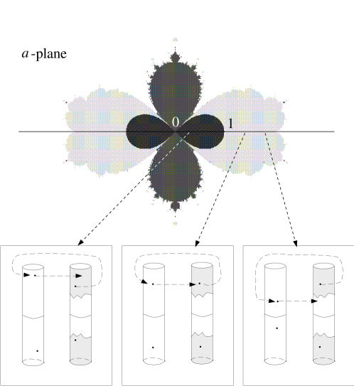
Figure 10. Lavaurs’ continuity argument

Theorem B.3.

In this setting, if $a_{k}\to a$ and $\epsilon_{k}\to 0$ such that

$$\varrho^{+}_{a_{k},\epsilon_{k}}\to\varrho^{+}_{a:\Theta}\;\mbox{ or equivalently }\;\varrho^{-}_{a_{k},\epsilon_{k}}\to\varrho^{-}_{a:\Theta}$$

then ${\cal F}_{a_{k},\epsilon_{k}}\to{\cal F}_{a:\Theta}$ locally uniformly on ${\cal W}_{a}$.

We are now in a position to avail ourselves of an elementary but crucial observation of Lavaurs [La]:

Lemma B.4.

There exist $a\in(0,\sqrt{3})$ and a transit map $\Theta:C^{\cal A}_{a}\to C^{\cal R}_{a}$ respecting equators, such that both $\Theta(\upsilon^{\pm}_{a})$ are superattracting fixed points for ${\cal F}_{a:\Theta}$.

The relevant continuity argument is depicted in Fig. B.4. For small $a>0$, the critical values $\upsilon^{+}_{a}$ and $\upsilon^{-}_{a}$ are farther apart than any pair of critical points of ${\cal E}_{a}$. All of these points move continuously as $a$ increases towards the parameter value $\sqrt{3}$ where $\upsilon_{a}^{\pm}$ collide at the equator. Consequently, there exist $a\in(0,\sqrt{3})$ and a symmetric pair of critical points $c_{a}^{\pm}$ which are exactly as far apart as the critical values $\upsilon_{a}^{\pm}$. Both possibilities

$${\cal E}_{a}(c_{a}^{\pm})=\upsilon_{a}^{\pm}\;\;\operatorname{and}\;\;{\cal E}_{a}(c_{a}^{\pm})=\upsilon_{a}^{\mp}$$

may be so arranged. Choosing the former, we see that $\Theta(\upsilon_{a}^{\pm})=c_{a}^{\pm}$ for a suitable transit map respecting equators; in particular, each of $c_{a}^{\pm}$ is a superattracting fixed point for ${\cal F}_{a:\Theta}$.

Let $a$ be the parameter value so obtained. In view of (B.2) there exist real $\epsilon_{k}$ decreasing to $0$ with $\varrho^{\pm}_{a,\epsilon_{k}}\to\varrho^{\pm}_{a:\Theta}$. It follows from Theorem B.3 that the nearby fixed points of of ${\cal F}_{a,\epsilon_{k}}$ are attracting. Their lifts generate a complex conjugate pair of attracting periodic orbits in the original dynamical plane, and thus $J(Q_{a,\epsilon_{k}})$ is connected; moreover, $Q_{a,\epsilon_{k}}$ is birenormalizable as the critical orbits are separated by the real-axis. The two ways of marking the critical points of $Q_{a}$ yield parameters $(A_{\infty},\pm D_{\infty})\in\operatorname{Per}_{1}(1)$ and corresponding parameters $(A_{k},\pm D_{k})\in\Phi_{0}({\cal M}-\{{\operatorname{root}}\})$ associated to the perturbations $Q_{a,\epsilon_{k}}$. It follows from (B.1) that $A_{\infty}<0$, and thus $(A_{\infty},\pm D_{\infty})$ are the endpoints of an interval $I$ on the simple arc

$${\cal P}=\{(A,D)\in\operatorname{Per}_{1}(1)|\;A<0\}.$$

The entire impression

$${\cal I}=\{(A,D)\in{\mathcal{C}}^{\#}_{{\mathbb{R}}}|\;\Psi_{0}(c_{j})\to(A,D)\mbox{ for some }c_{j}\in{\cal M}\setminus\{{\operatorname{root}}\}\mbox{ with }c_{j}\to{\operatorname{root}}\}$$

lies in $\cal P$ by Yoccoz Inequality (2.1); thus $I\subset{\cal I}$, as $\cal I$ is connected and

$$(A_{\infty},\pm D_{\infty})=\lim_{k\to\infty}(A_{k},\pm D_{k})\in{\cal I}$$

by construction. It follows from Lemma 2.3 and the considerations of Lemma A.1 that ${\mathcal{C}}^{\#}_{{\mathbb{R}}}$ is non-locally connected at every $(A,D)\in{\cal I}$ for which $P_{A,D}$ has a parabolic-repelling fixed point.

References

- [Bi1] B. Bielefeld, Changing the order of critical points of polynomials using quasiconformal surgery, Thesis, Cornell, 1989.
- [Bi2] B. Bielefeld, Questions in quasiconformal surgery, pp. 2-8, in Conformal Dynamics Problem List, ed. B. Bielefeld, Stony Brook IMS Preprint 1990/1, and in part 2 of Linear and Complex Analysis Problem Book 3, ed. V. Havin and N. Nikolskii, Lecture Notes in Math. 1574, Springer-Verlag, 1994.
- [BD] B. Branner and A. Douady, Surgery on complex polynomials, in Proceedings of the Symposium on Dynamical Systems, Mexico, 1986, Lecture Notes in Math. 1345, Springer-Verlag, 1987.
- [BF] B. Branner and N. Fagella, Homeomorphisms between limbs of the Mandelbrot set, MSRI Preprint 043-95.
- [BH] B. Branner and J.H. Hubbard, The iteration of cubic polynomials. Part I: The global topology of parameter space, Acta Mathematica, 160 (1988), 143-206.
-
[Bu]
X. Buff,
Extension d’homéomorphismes de compacts de ,
Manuscript,
and personal communication. - [Do] A. Douady. Does a Julia set depend continuously on a polynomial?, Proc. of Symp. in Applied Math. 49 (1994).
- [DH1] A. Douady and J.H. Hubbard, Étude dynamique des polynômes complexes, I& II, Publ. Math. Orsay (1984-5).
- [DH2] A. Douady and J.H. Hubbard,On the dynamics of polynomial-like mappings, Ann. scient. Éc. Norm. Sup., série, 18 (1985), 287-343.
- [Ep] A. Epstein, Counterexamples to the quadratic mating conjecture, Manuscript in preparation.
- [Fa] D. Faught, Local connectivity in a family of cubic polynomials, Thesis, Cornell 1992.
- [GM] L. Goldberg and J.Milnor, Fixed points of polynomial maps II, Ann. Scient. Éc. Norm. Sup., série, 26 (1993), 51-98.
- [Haï] P. Haïssinsky, Chirurgie croisée, Manuscript, 1996.
- [Hub] J.H. Hubbard, Local connectivity of Julia sets and bifurcation loci: three theorems of J.-C. Yoccoz, in Topological methods in Modern Mathematics, Publish or Perish, 1992, pp. 467-511 and 375-378.
- [Ki] J. Kiwi, Non-accessible critical points of Cremer polynomials, IMS at Stony Brook Preprint 1995/2.
- [La] P. Lavaurs, Systèmes dynamiques holomorphes: Explosion de points périodiques, Thèse, Université de Paris-Sud, 1989.
- [LV] O. Lehto and K. I. Virtanen, Quasiconformal Mappings in the Plane, Springer-Verlag, 1973.
- [Lyu1] M. Lyubich, On typical behavior of the trajectories of a rational mapping of the sphere, Soviet. Math. Dokl., 27 (1983), 1, 22-25.
- [Lyu2] M. Lyubich, On the Lebesgue measure of a quadratic polynomial, IMS at Stony Brook Preprint 1991/10.
- [Lyu3] M. Lyubich, Dynamics of quadratic polynomials, I. Combinatorics and geometry of the Yoccoz puzzle, MSRI Preprint 026-95.
- [MSS] R. Mañé, P. Sad and D. Sullivan, On the dynamics of rational maps, Ann. Scient. Éc. Norm. Sup., série, 16 (1983), 51-98.
- [McM1] C. McMullen, Complex Dynamics and Renormalization, Annals of Math. Studies, Princeton Univ. Press, 1993.
- [McM2] C. McMullen, Renormalization and 3-Manifolds which Fiber over the Circle, Annals of Math. Studies, Princeton Univ. Press, 1996.
- [McS] C. McMullen and D. Sullivan, Quasiconformal homeomorphisms and dynamics III: The Teichmüller space of a rational map, Preprint, 1996.
- [Mil1] J. Milnor, Dynamics in one complex variable: Introductory lectures, IMS at Stony Brook Preprint 1990/5.
- [Mil2] J. Milnor, Remarks on iterated cubic maps, IMS at Stony Brook Preprint 1990/6.
- [Mil3] J. Milnor, On cubic polynomials with periodic critical point. Manuscript, 1991.
- [Mil4] J. Milnor, Hyperbolic components in spaces of polynomial maps, with an appendix by A. Poirier, IMS at Stony Brook Preprint 1992/3.
- [Mil5] J. Milnor, Periodic orbits, external rays and the Mandelbrot set; An expository account, Preprint, 1995.
- [NS] S. Nakane and D. Schleicher, Non-local connectivity of the tricorn and multicorns, in Proceedings of the International Conference on Dynamical Systems and Chaos, World Scientific, 1994.
- [Sh] M. Shishikura, The parabolic bifurcation of rational maps, Colóquio Brasileiro de Matemática 19, IMPA, 1992.
- [Win] R. Winters, Bifurcations in families of antiholomorphic and biquadratic maps, Thesis, Boston University, 1989.
- [Yar] B. Yarrington, Local connectivity and Lebesgue measure of polynomial Julia sets, Thesis, SUNY at Stony Brook, 1995.