Dynamics of the family $\lambda\tan z$

Abstract

We study the the tangent family ${\cal F}=\{\lambda\tan z,\lambda\in{\mathbb{C}}-\{0\}\}$ and give a complete classification of their stable behavior. We also characterize the the hyperbolic components and give a combinatorial description their deployment in the parameter plane.

Published in modified form: Conf. Geom. & Dynam. 1 (1997), 28–57 Stony Brook IMS Preprint #1995/8 May 1995 Revised version: June 1997

1 Introduction

One of the central questions in conformal dynamics is characterizing, in “natural” families of meromorphic functions such as $\{z^{2}+\lambda,\lambda\in{\mathbb{C}}\}$, those members that define hyperbolic dynamical systems. The Mandelbrot set shows how the hyperbolic systems fall into connected components of the parameter plane. Systems within a given component are topologically conjugate and the combinatorial structure of these components has been studied in detail by many people. McMullen’s survey, [15], and the references therein provide a good introduction to this work.

Transcendental meromorphic functions, and $\tan z$ in particular, offer another interesting one complex dimension domain to study. The dynamical properties of the tangent family were first studied by Devaney and Keen in [10, 11] and pursued by Baker, Kotus, and Lü in [2, 3, 4, 5]. W.H. Jiang did the computer studies of the parameter plane in figures 1,2 and 3 as part of his unpublished thesis [13]. These figures were the motivation for our work.

In the quadratic family, one can show that each hyperbolic component in the parameter plane contains a unique point (its “center”) that has a superattractive periodic cycle. One can enumerate these centers in terms of a combinatorial description of their dynamical behavior. Since $\lambda\tan z$ has no critical points, and so no superattractive cycles, we need another way to enumerate its hyperbolic components. We use parameter values for which the asymptotic values eventually land on a pole. We call these parameter values virtual centers, which is an apt term dynamically, but a little dicey geometrically, because they turn out to lie on the boundary of the hyperbolic components. We shall see that for each $\lambda$, there is a natural map from the prepoles of $\lambda\tan z$ to the set of virtual centers. We use this correspondence to characterize the hyperbolic components.

The paper is organized as follows. In section 2, we give the basic facts about iteration of meromorphic functions. In section 3, we discuss the concepts of quasiconformal stability and J-stability of meromorphic functions in terms of extensions of holomorphic motions [17, 16]. In section 4, we give the special properties of the tangent family ${\cal F}$ and in section 5, we classify the stable behavior of its functions. In addition, we characterize the connectivity properties of the Julia sets of functions in ${\cal F}$ for various values of the parameter $\lambda$. In section 6, we give an alternative characterization for the Julia set of the tangent functions as the closure of the set of prepoles. We describe the combinatorial structure of the prepoles and of the periodic points. In section 7 we prove that for the tangent family, the set of J-stable parameters coincides with the set of quasiconformally stable parameters. In sections 8 and 9 we describe the deployment of the hyperbolic components and establish the correspondence between the prepoles and virtual centers. We exploit this correspondence, together with the results in section 6, to transfer properties from the dynamic plane to the parameter plane to obtain the combinatorial picture of the hyperbolic components.

The authors wish to thank Anna Zdunik for reading preliminary versions of this paper and for her helpful comments. They would also like to thank Scott Sutherland for his help with the figures. In addition, they thank the referee for his suggestions for improving the exposition and for finding errors in our proof of the density conjecture in earlier versions of this paper. The second author would like to acknowledge the hospitality of the Graduate Center at CUNY and the Institute of Mathematical Sciences at SUNY Stony Brook. Finally, both authors thank the Mathematical Sciences Research Institute for its support.

2 Basics

2.1 Meromorphic functions

If $f$ is a meromorphic function, the orbits of points fall into three categories: they may be infinite, they may become periodic and hence consist of a finite number of distinct points, or they may terminate at a pole of $f$. For transcendental meromorphic functions with more than one pole, it follows from Picard’s theorem that the set of prepoles, that is, ${\cal P}=\cup_{n=0}^{\infty}{f^{\circ-n}}(\infty)$ is infinite. To study the dynamics, we define the stable set, or Fatou set, $F_{f}$ as the set of those points $z$ such that the sequence ${f^{\circ n}}(z)$ is defined and meromorphic for all $n$, and forms a normal family in a neighborhood of $z$. The unstable set, or Julia set, $J_{f}$ is the complement of the Fatou set. Thus $F_{f}$ is open, $J_{f}$ is closed and $\bar{\cal P}\subset J_{f}$ so that $J_{f}\neq\emptyset$. It is easy to see that both $F_{f}$ and $J_{f}$ are completely invariant.

Meromorphic functions may have values $z\in\hat{\mathbb{C}}$ with finite backward orbit. These constitute the exceptional set $E_{f}$. By Picard’s theorem, $|E_{f}|\leq 2$ and $\infty\not\in E_{f}$. As for rational functions, for any $z\in\hat{\mathbb{C}}-E_{f}$, $J_{f}\subset\overline{\cup_{n=0}^{\infty}{f^{\circ-n}}(z)}$ and if $z\in J_{f}$, $J_{f}=\overline{\cup_{n=0}^{\infty}{f^{\circ-n}}(z)}$. It follows that $J_{f}=\overline{{\cal P}}$, a fact which is essential to our proofs. We also may characterize $J_{f}$, as we do for rational maps, as the closure of the repelling periodic points [10, 3].

The singular set $S_{f}$ of a meromorphic function $f$ consists of those values at which $f$ is not a regular covering. Therefore at a singular value $v$ there is a branch of the inverse which is not holomorphic but has an algebraic or transcendental singularity. If the singularity is algebraic $v$ is a critical value whereas if it is transcendental, there is a path $\alpha:[0,\infty)\rightarrow{\bf C}$ such that $\lim_{t\to\infty}|\alpha(t)|=\infty$ and $\lim_{t\to\infty}f(\alpha(t))=v$; in this case $v$ is called an asymptotic value for $f$. If we can associate to a given asymptotic value $v$ an asymptotic tract, that is, a simply connected unbounded domain $A$ such that $f(A)$ is a punctured neighborhood of $v$, then $v$ is called a logarithmic singularity. Note that logarithmic singularities and critical values may belong to the Fatou set. The functions in the tangent family ${\cal F}$ have no critical points and so the singular set consists of asymptotic values which, in this case, are the points $\pm\lambda i$ of the exceptional set. These are logarithmic singularities with asymptotic tracts contained in the upper and lower half planes respectively.

Let $D$ be a component of the Fatou set; $f$ maps $D$ to a component, but if the image contains an asymptotic value, the map may not be onto. In any case, we call the image component $f(D)$ and note the dichotomy:

• there exist integers $m\neq n>0$ such that ${f^{\circ n}}(D)={f^{\circ m}}(D)$, and $D$ is called eventually periodic, or

• for all $m\neq n$, ${f^{\circ n}}(D)\cap{f^{\circ m}}(D)=\emptyset$, and $D$ is called a wandering domain.

The qualitative and quantitative description of the eventually periodic stable behavior of meromorphic functions is slightly more complicated than that of rational maps because of the essential singularity at $\infty$ and the possibility that $f^{p}$ may not be defined at some values. Suppose $z_{0},z_{1}=f(z_{0}),\ldots,z_{p}=f(z_{p-1})=z_{0}$ is a periodic cycle for $f$. The eigenvalue or multiplier of the cycle is defined to be $\alpha=({f^{\circ p}})^{\prime}(z_{i})$, $i=0,\ldots,p-1$.

Suppose now that the domain $D$ lands on a periodic cycle of domains $D_{0},D_{1},\ldots D_{p-1}$; then either

1. $D_{i}$ is attractive: each $D_{i}$ contains a point of a periodic cycle with eigenvalue $|\alpha|<1$ and all points in the $D_{i}$ are attracted to this cycle. Some domain in this cycle must contain a critical or an asymptotic value. If $|\alpha|=0$, the critical point itself belongs to the periodic cycle and the domain is called superattractive.

2. $D_{i}$ is parabolic: the boundary of each $D_{i}$ contains a point of a periodic cycle with eigenvalue $\alpha=e^{2\pi ip/q}$, $(p,q)=1$, and all points in the domains $D_{i}$ are attracted to this cycle. Some domain in this cycle must contain a critical or an asymptotic value.

3. $D_{i}$ is a Siegel disk: each $D_{i}$ is contains a point of a periodic cycle with eigenvalue $\alpha=e^{2\pi i\theta}$ where $\theta$ is irrational. There is a holomorphic homeomorphism mapping each $D_{i}$ to the unit disk $\Delta$, and conjugating the first return map ${f^{\circ p}}$ on $D_{i}$ to an irrational rotation of $\Delta$. The preimages under this conjugacy of the circles $|\zeta|=r,\,r<1$ foliate the disks $D_{i}$ with ${f^{\circ p}}$ forward invariant leaves on which ${f^{\circ p}}$ is injective.

4. $D_{i}$ is a Herman ring: each $D_{i}$ is holomorphically homeomorphic to a standard annulus and the first return map is conjugate to an irrational rotation of the annulus by the holomorphic homeomorphism. The preimages under this conjugacy of the circles $|\zeta|=r,\,1<r<R$ foliate the disks with ${f^{\circ p}}$ forward invariant leaves on which ${f^{\circ p}}$ is injective.

5. $D_{i}$ is an essentially parabolic or Baker domain: the boundary of each $D_{i}$ contains a point $z_{i}$ (possibly $\infty$), ${f^{\circ np}}(z)\to z_{i}$ for all $z\in D_{i}$, but ${f^{\circ p}}$ is not holomorphic at $z_{i}$. If $p=1$, then $z_{0}=\infty$ .

   For examples of essentially parabolic domains with $p\neq 1$ and $z_{i}\neq\infty$ see [2].

Definition:  A meromorphic map $f$ is called hyperbolic if it is expanding on its Julia set; that is, there exist constants $c>0$ and $K>1$ such that for all $z$ in a neighborhood $V\supset J$, $|({f^{\circ n}})^{\prime}(z)|>cK^{n}$.

3 Quasiconformal Conjugacy and J-stability

An effective method for studying the analytic structure of the parameter space of a family of rational maps or meromorphic functions with finite singular set is to use the theory of holomorphic motions. This is presented in detail for rational maps in [16]. We indicate here how to adapt it for meromorphic functions with finite singular set. This is not substantially harder than restricting ourselves to the tangent family ${\cal F}$ and gives a more general result.

Definitions:

• A holomorphic family of meromorphic maps $f_{x}(z)$ over a complex manifold $X$ is a holomorphic map $X\times\hat{\mathbb{C}}\rightarrow\hat{\mathbb{C}}$, given by $(x,z)\mapsto f_{x}(z)$.

• A point $x_{0}\in X$ is topologically stable if there is a neighborhood $U$ of $x_{0}$ such that for all $y\in U$ there is a homeomorphism $\phi:\hat{\mathbb{C}}\to\hat{\mathbb{C}}$ such that $f_{y}=\phi^{-1}\circ f_{x_{0}}\circ\phi$. Denote by $X^{top}\subset X$ the subset of topologically stable parameters.

• The subset $X^{qc}\subset X^{top}$ is defined similarly, except that $\phi$ is required to be quasiconformal.

• The subset $X^{post}\subset X$ of postsingularly stable points consists of those parameter values for which the combinatorial properties of the singular values is locally constant; that is, in a neighborhood of $x\in X^{post}$, any relations among the forward orbits of the singular values of $f_{x}$ persist. For $x\in X^{post}$ the singular points are locally defined distinct holomorphic functions of $x$. Clearly, $X^{post}$ is open and dense in the subset of $X$ on which the number of singular values counted without multiplicity is constant and $X^{top}\subset X^{post}$.

• A holomorphic motion of a set $V\subset\hat{\mathbb{C}}$ over a connected complex manifold with basepoint $(X,x_{0})$ is a map $\phi:X\times V\rightarrow\hat{\mathbb{C}}$ given by $(x,v)\mapsto\phi_{x}(v)$ such that

  1. for each $v\in V$, $\phi_{x}(v)$ is holomorphic in $x$,

  2. for each $x\in V$, $\phi_{x}(v)$ is an injective function of $v\in V$, and,

  3. at $x_{0}$, $\phi_{x_{0}}=v(x_{0})$.

• A holomorphic motion over a holomorphic family respects the dynamics if $\phi_{x}(f_{x_{0}}(v))=f_{x}(\phi_{x}(v))$ whenever both $v$ and $f_{x}(v)$ belong to $V$.

• The set $X^{stab}$ of J-stable parameters is the subset of $X$ where the Julia set moves by a holomorphic motion respecting the dynamics.

The following theorem is proved in [17] (Theorem B). We state it here as it applies in our context:

Theorem 3.1

In any holomorphic family of meromorphic maps with finite singular set defined over the complex manifold $X$, the set of J-stable parameters coincides with the set on which the total number of attracting and superattracting cycles of $f_{x}$ is constant on a neighborhood of $x$.

As a corollary we have:

Corollary 3.2

The J-stable parameters are open and dense in $X$.

Proof:   Let $N(x)$ be the number of attracting cycles of $f_{x}$. By Fatou [12] the set on which $N(x)$ is a local maximum is open and dense. By the above theorem, this set coincides with $X^{stab}$. $\;\square$

The following theorem is proved in [16] for rational maps, but the proof works just as well for meromorphic maps with finite singular set.

Theorem 3.3

In any holomorphic family of meromorphic maps with finite singular set defined over the complex manifold $X$, $X^{qc}=X^{top}$ and $X^{qc}$ is open and dense.

Proof:   Fix $x_{0}\in X^{post}$ and let $Y$ be a neighborhood of $x_{0}$ on which the combinatorics of the singular values are constant. Define a holomorphic mapping $\phi:Y\times S_{f_{x_{0}}}\rightarrow{\bf C}$ by $(x,v)\mapsto\phi_{x}(v)=v(x)$. Note that $\phi$ is a holomorphic motion because the singular values move injectively.

Since the combinatorics of the singular values are constant in $Y$, the extension of the motion to the forward orbits of the singular values by

$$\phi_{x}(f_{x_{0}}(v))=f_{x}(\phi_{x}(v))$$

is well defined, injective and depends holomorphically on $x$. Next, we can extend this motion to the grand orbits of the singular values. Again, the persistence of the orbit relations is precisely what is needed to do this so that the appropriate inverse branch can be uniquely chosen by analytic continuation. Indeed, suppose that $FS_{f_{x}}$ is the post-singular set and that $\phi_{x}(z)$ is defined for some $z\in FS_{f_{x}}$ and $x\in Y$. To show that the inverse branches are holomorphic single-valued functions defining a holomorphic function of $f_{x}^{-1}(\phi_{x}(z))$ we consider the graph

$$G=\{(x,w)|f_{x}(w)=\phi_{x}(z)\}$$

defined by the preimages and show that the cardinality of the preimage is constant on each component.

If $z$ is a critical value, its critical preimages $c_{i_{1}},\ldots c_{i_{k}}$ have constant multiplicity in $Y$ and each defines a component of $G$ with cardinality given by the multiplicity. Non-critical preimages map injectively and define components whose cardinality is one. If $z$ is an asymptotic value, the number of asymptotic tracts is constant in $Y$; these “omitted” preimages do not contribute components to $G$, but the number of such “missing components” is constant. Consequently, the cardinality of the preimage is constant on components.

Now we are ready to extend $\phi_{x}$ to all of $\hat{\mathbb{C}}$, albeit on a neighborhood $U\subset Y$, one-third the size of $Y$, so that for each $x\in U$, $\phi_{x}$ is quasiconformal and respects the dynamics. The Bers-Royden harmonic $\lambda$-lemma [6] asserts the existence of a unique quasiconformal extension, $\phi:U\times\hat{\mathbb{C}}\rightarrow\hat{\mathbb{C}}$ with the property that its Beltrami differential for each $x\in U$, $\phi_{\bar{z}}/\phi_{z}$, is harmonic. We claim that the Bers-Royden extension $\phi$ respects the dynamics; that is $\phi_{x}=f_{x}^{-1}\circ\phi_{x}\circ f_{x_{0}}$. Set $\psi_{x}(z)=f_{x}^{-1}\circ\phi_{x}\circ f_{x_{0}}(z)$ where the branch of the inverse is chosen by continuation so that $\psi_{x_{0}}(z)=z$. On the post-singular set, by construction, $\psi_{x}(z)=\phi_{x}(z)$ already. Since $f_{x_{0}}$ and $f_{x}$ are conformal, by the chain rule, the Beltrami coefficient of $\psi_{x}$ is the pullback of the harmonic Beltrami coefficient of $\phi_{x_{0}}$. Moreover, since $f_{x_{0}}$ is a hyperbolic isometry off the post-singular set, the Poincaré metric is invariant under the pullback. It follows that the Beltrami differential of $\psi_{x}$ is again harmonic and by the uniqueness of the Bers-Royden extension $\phi_{x}=\psi_{x}$. Thus $\phi$ respects the dynamics and $x_{0}\in X^{qc}$.

Therefore we have proved, $X^{post}\subset X^{qc}$. Since by definition, $X^{qc}\subset X^{top}\subset X^{post}$, we conclude $X^{post}=X^{top}=X^{qc}$. $\;\square$

4 The family ${\cal F}$

4.1 Topological characterization

The family ${\cal F}=\{f_{\lambda}=\lambda\tan z\}$ is a holomorphic family over the punctured complex plane $X={\bf C}-\{0\}$. The discussion below shows that it is also topologically closed in the following sense: if $g$ is topologically conjugate to $f_{\lambda}\in{\cal F}$ then $g$ is affine conjugate to $f_{\lambda}$.

Functions with constant Schwarzian derivative $2k$ have two asymptotic values and no critical points. If $f$ is such a function it has the form

$$f(z)=\frac{Ae^{2kz}+B}{Ce^{2kz}+D},\,\,\,A,B,C,D\in{\mathbb{C}},\,\,AD-BC\neq 0$$

and the asymptotic values are $A/C$ and $B/D$. This follows from the following fundamental theorem of Nevanlinna ([19], chap. XI, see also [10, 11]).

Theorem 4.1 (Nevanlinna)

Meromorphic maps whose Schwarzian derivative is a polynomial of degree $p-2$ are exactly those functions which have $p$ logarithmic singularities $a_{0},a_{1},\ldots,a_{p-1}$. The $a_{i}$ need not be distinct. There are exactly $p$ disjoint sectors $W_{0},\ldots,W_{p-1}$ at $\infty$, each with angle $\frac{2\pi}{p}$, and a collection of disks $B_{i}$, one around each $a_{i}$, satisfying:

$f^{-1}(B_{i}-\{a_{i}\})$ contains a unique unbounded component $U_{i}$, contained in $W_{i}$, called its asymptotic tract, and
$f:U_{i}\mapsto B_{i}-\{a_{i}\}$ is a universal covering.

We have, as almost immediate corollaries to this theorem (see [11] for proof).

Corollary 4.2

If $f$ has constant Schwarzian derivative $2k$ and if its asymptotic values are $0$ and $\infty$ then $f(z)=\lambda e^{kz}$ for some $\lambda\in{\mathbb{C}}$.

Corollary 4.3

If $f$ has constant Schwarzian derivative $2k$ and if its asymptotic values are symmetric with respect to the origin and $0$ is fixed then $f(z)=\lambda\tan z$ for some $\lambda\in{\mathbb{C}}$ and $f\in{\cal F}$ and the asymptotic values are $\pm\lambda i$.

In addition we have the topological closure of the tangent family,

Corollary 4.4

If $g(z)$ is topologically conjugate to $f(z)=\lambda\tan z$, then $g(z)$ is affine conjugate to $\lambda^{\prime}\tan z$ for some $\lambda^{\prime}$. Moreover, if $\phi(\lambda i)=-\phi(-\lambda i)$, then $g(z)=\lambda^{\prime}\tan z$.

Proof:   Let $g=\phi\circ f\circ\phi^{-1}$ and set $J(z)=-z$. Then since $f=J^{-1}\circ f\circ J$, $g=\phi\circ J\circ\phi^{-1}\circ g\circ\phi\circ J^{-1}\circ\phi^{-1}$. Now by theorem 3.3 we may assume $\phi$ is quasiconformal. Therefore, $\hat{J}=\phi\circ J\circ\phi^{-1}$ is a holomorphic homeomorphism of ${\mathbb{C}}$ of order $2$ and so must have the form $\hat{J}=-z+b$ for some $b\in{\mathbb{C}}$.

Topological conjugation preserves the asymptotic values so $v=\phi(\lambda i)$ and $v^{\prime}=\phi(-\lambda i)$ are the asymptotic values of $g$. Since $J$ exchanges the asymptotic values of $f$, $\hat{J}(v)=v^{\prime}$. By hypothesis, $v^{\prime}=-v$ so that $b=0$, $\hat{J}(z)=-z$ and $g(0)=-g(0)=0$. Applying corollary 4.3 we are done. $\;\square$

Remark 4.1

If $f$ has constant Schwarzian derivative $2k$ and if its asymptotic values are equal, then $k=0$ and $f$ is constant; since it fixes the origin, $f\equiv 0$.

4.2 Symmetry

The symmetry of the maps in ${\cal F}$ with respect to $0$ implies that the stable and unstable sets are respectively symmetric with respect to the origin. Precisely,

Proposition 4.5

For $f_{\lambda}\in{\cal F}$,

1. $z\in J_{\lambda}$ if and only if $-z\in J_{\lambda}$, hence $z\in F_{\lambda}$ if and only if $-z\in F_{\lambda}$, and

2. $z\in J_{\lambda}$ if and only if $z\in J_{-\lambda}$ hence $z\in F_{\lambda}$ if and only if $z\in F_{-\lambda}$.

Proof:   For $z\in{\mathbb{C}}$ we have

$$f_{\lambda}(-z)=-f_{\lambda}(z),$$

so for all $k\in{\mathbb{N}}$,

$${f^{\circ k}_{\lambda}}(-z)=-{f^{\circ k}_{\lambda}}(z),\,\mbox{and }\,[{f^{\circ k}_{\lambda}}(-z)]^{\prime}=[{f^{\circ k}_{\lambda}}(z)]^{\prime}.$$

It follows that if ${f^{\circ p}_{\lambda}}(z)=z$, then ${f^{\circ p}_{\lambda}}(-z)=-z.$ Moreover if $z_{0},\ldots z_{p-1}$ is a periodic cycle of period $p$ then either $p$ is even and $-z_{0},\ldots,-z_{p-1}$ is a cyclic permutation of the former cycle, or it is a distinct cycle of period $p$ and $p$ may be either odd or even. The symmetry also implies that if $z$ is a repelling, attracting, parabolic, or irrational neutral periodic point (stable or unstable), $-z$ has the same property. Note that there are never superattracting cycles because there are no critical points. Since the Julia set is the closure of the repelling periodic points, we can say that $z\in J_{\lambda}$ if and only if $-z\in J_{\lambda}$. Consequently $z\in{F}_{\lambda}$ if and only if $-z\in{F}_{\lambda}$. In particular, if $\lambda i\in{F}_{\lambda}$ then $-\lambda i\in{F}_{\lambda}$ and the orbits $\{{f^{\circ n}}_{\lambda}(\lambda i)\}$ and $\{{f^{\circ n}}_{\lambda}(-\lambda i)\},\,n\in{\mathbb{N}}$ are symmetric; they either belong to the immediate basin associated to one attracting (or parabolic) cycle of even period or they belong to two distinct symmetric attracting (or parabolic) cycles of $z$ and $-z$. Note that in both cases the immediate basins are symmetric.

To prove 2. we note that for $z\in{\mathbb{C}}$ and $k\in{\mathbb{N}}$

$${f^{\circ k}_{-\lambda}}(z)=(-1)^{k}{f^{\circ k}_{\lambda}}(z)\,\,\mbox{and}\,\,f_{\lambda}(-z)=f_{-\lambda}(z).$$

So if $p$ is even

$${f^{\circ p}_{\lambda}}(z)=z\,\,\mbox{implies}\,\,{f^{\circ p}_{-\lambda}}(z)=z,$$

while if $p$ is odd

$${f^{\circ p}_{\lambda}}(z)=z\,\,\mbox{implies}\,{f^{\circ 2p}_{-\lambda}}(z)=z.$$

If $p$ is odd, this means that if $z_{0},\ldots z_{p-1}$ and $-z_{0},\ldots-z_{p-1}$ are distinct cycles for $f_{\lambda}$, they belong to the same cycle for $f_{-\lambda}$ but the cycle has double the period. For $p$ even the same may be true, but there is another possibility: $f_{-\lambda}$ may still have two distinct cycles but they are now $z_{0},-z_{1},z_{2},\ldots,z_{p-2},-z_{p-1}$ and $-z_{0},z_{1},-z_{2},\ldots,-z_{p-2},z_{p-1}$.

Since

$$[{f^{\circ k}_{-\lambda}}(z)]^{\prime}=(-1)^{k}[{f^{\circ k}_{\lambda}}(z)]^{\prime}\,\,\mbox{for}\,\,\,k\in{\mathbb{N}},$$

if $z$ is a repelling, attracting, parabolic, or irrational neutral periodic point of $f_{\lambda}$, then $z$ is a periodic point of the same type for $f_{-\lambda}$ (with possibly double or half the period). To complete the proof we again use the property that the Julia set is the closure of the repelling periodic points and the classification of periodic stable behavior. $\;\square$

Remark 4.2

We see that although the map $J(z)=-z$ satisfies $J\circ f_{\lambda}=f_{\lambda}\circ J$ for all $\lambda$, it does not conjugate the dynamics of $f_{\lambda}$ and $f_{-\lambda}$ because distinct symmetric cycles of period $p$ of $f_{\lambda}$ often (but not always) become single cycles of period $2p$ of $f_{-\lambda}$ and vice versa. The map $j(z)=\bar{z}$, on the other hand, conjugates $f_{\lambda}$ to $f_{\bar{\lambda}}$ and conjugates the dynamics properly.

4.3 Inverse branches

The function $\tan z$ is periodic with period $\pi$ and so is an infinite to one cover of $\hat{\mathbb{C}}-\{\pm\lambda i\}$. The origin is a fixed point and the points $q_{n}=n\pi$, $n=\pm 1,\pm 2,\ldots$ are also preimages of the origin. The poles are $s_{n}=(n+1/2)\pi$, $n=\pm 1,\pm 2,\ldots$; the image of the real line between any pair of poles is the whole real line. The image of the imaginary axis and its translates by $\pi$ is the vertical segment of the imaginary axis between $i$ and $-i$; the image of the vertical lines $l_{n}=(n+1/2)\pi+it,t\in{\mathbb{R}},n\in{\mathbb{Z}}$ is the pair of segments of the imaginary axis above and below $\pm i$. We denote by $L_{n}$ the half open vertical strip between the lines $l_{n-1}$ and $l_{n}$ and containing the line $l_{n-1}$. From the above, we see that it is divided into four quadrants, each a preimage of the corresponding quadrant in ${\mathbb{C}}$. The function $f_{\lambda}=\lambda\tan z$ therefore maps each strip $L_{n}$ onto $\hat{\mathbb{C}}-\{\pm\lambda i\}$ and takes the quadrants in $L_{n}$ onto the quadrants of ${\mathbb{C}}$ formed by multiplying the real and imaginary axes by $\lambda i$.

The inverse map of $f_{\lambda}$ is given by the following formula

$$f^{-1}_{\lambda}(z)=\frac{1}{2i}\log\left(\frac{\lambda+iz}{\lambda-iz}\right).$$ (1)

Let $\lambda=a_{1}+ia_{2},z=x+iy$ then

$$\Re f_{\lambda}^{-1}(z) = \frac{1}{2}\arctan\left(\frac{2a_{1}x+2a_{2}y}{|\lambda|^{2}-|z|^{2}}\right)$$ (2)

$$\Im f_{\lambda}^{-1}(z) = -\frac{1}{4}\log\left(\frac{(|\lambda|^{2}-|z|^{2})^{2}+(2a_{1}x+2a_{2}y)^{2}}{[(a_{1}+y)^{2}+(a_{2}-x)^{2}]^{2}}\right),$$ (3)

where in equation (2) we must specify which branch of the $\arctan$ we use. We therefore denote by $f_{n,\lambda}^{-1}$ (or $f_{n}^{-1}$ if no confusion will result) the branch of the inverse map whose real part is in the strip $L_{n}$. For a given $p\in{\mathbb{N}}$ we define a branch of $f^{-p}_{\lambda}$ by

$$f_{{\bf n}_{p},\lambda}^{-p}=f^{-1}_{n_{p},\lambda}\circ\cdots\circ f^{-1}_{n_{2},\lambda}\circ f^{-1}_{n_{1},\lambda},$$ (4)

and set ${\bf n}_{p}=(n_{1},n_{2},\ldots,n_{p})$. We call ${\bf n}_{p}$ the itinerary of the map $f_{{\bf n}_{p},\lambda}^{-p}$.

5 The Dynamic Plane: the Fatou set $F_{\lambda}$

The maps in ${\cal F}$ have no critical points so there are no superattracting cycles. Moreover, it follows from [11] that functions in ${\cal F}$, have no essentially parabolic domains. In this section we shall prove that no function in the family ${\cal F}$ can have a Herman ring. In [11] and in [5] it is proved that maps in ${\cal F}$ have no wandering domains. The stable behavior for functions in ${\cal F}$ is therefore either eventually attractive, parabolic, or lands on a cycle of Siegel disks.

It therefore follows, just as for rational maps that an equivalent characterization of hyperbolicity for maps in ${\cal F}$ is (see e.g. [18]):

Proposition 5.1

A map in ${\cal F}$ is hyperbolic if and only if the closure of its post-singular set, $\overline{\cup_{n\geq 0,v\in S_{f}}{f^{\circ n}}(v)}$, is disjoint from its Julia set.

In analogy with the situation for rational maps, we shall prove the following dichotomy exists:

Theorem 5.2

For $f_{\lambda}\in{\cal F}$ either

• $|\lambda|<1$, the Julia set $J_{\lambda}$ is locally a Cantor set and the Fatou set consists of a single infinitely connected invariant component, or

• $|\lambda|\geq 1$, the the Julia set $J_{\lambda}$ is connected and the Fatou set consists of either exactly two or infinitely many simply connected components.

Let $D_{0},D_{1}$ be components of the Fatou set with $f:D_{0}\to D_{1}$, where for readability, and provided there is no ambiguity, we omit the subscript $\lambda$. Since there are no critical points, $f|_{D_{0}}$ is a covering of its image and the degree is either 1 or infinite.

Proposition 5.3

If the degree of $f|_{D_{0}}$ is infinite then $D_{0}$ is unbounded.

Proof:   Suppose $D_{0}$ is bounded and let $\zeta$ be some point in $f(D_{0})$. Let $w\in\partial{D_{0}}$ be an accumulation point of $P=\{z_{n}=f^{-1}_{n}(\zeta),\,n\in\bf Z\}$. Choose a subsequence $z_{n_{j}}\in P$ such that $z_{n_{j}}\to w$. Then, since $f$ is analytic and $f(z_{n_{j}})=\zeta,\,f(w)=\zeta.$ This, however, contradicts the invariance of the Fatou set. $\;\square$

It follows that if the degree of $f|_{D_{0}}$ is 1 then $f(D_{0})=D_{1}$, while if the degree is infinite and if $D_{1}$ contains an asymptotic value, then $D_{0}$ contains an asymptotic tract and $f$ is a infinite degree covering map from the asymptotic tract onto a punctured neighborhood of the asymptotic value.

Corollary 5.4

Any attractive or parabolic cycle of components contains an unbounded component.

Proof:   Some component of the periodic cycle must contain an asymptotic value hence its preimage contains an asymptotic tract. $\;\square$

An immediate corollary is

Corollary 5.5

Any completely invariant component is unbounded.

Remark 5.1

It was proved in [4] that a transcendental meromorphic function with finitely many singular values has a maximum of two completely invariant components. Moreover, if $F_{\lambda}$ has two completely invariant components then each is simply connected. If the number of components of $F$ were finite, each would be completely invariant under a high enough iterate and so the number of components of $F$ is 1,2, or infinity.

Proposition 5.6

The connectivity of any component in the immediate basin of attraction of an attracting cycle is either 1 or infinity. For a parabolic cycle it is 1.

Proof:   Let $D_{0}$ be such a component, and let $z_{0}$ be an attractive periodic point in $D_{0}$ with first return map $f^{p}$. Let $U$ be a neighborhood of $z_{0}$ on which the linearization is defined and set $U_{n}=f^{-(np)}(U_{n-1})\cap D_{0}$. If the connectivity of $D_{0}>1,$ there is a $k$ such that the connectivity of $U_{n}>1$ for all $n>k.$ Since the degree of $f^{p}$ is infinite, the connectivity of $U_{n}$ is infinity and $D_{0}$ is infinitely connected.

Now consider the petals of the immediate basin of a parabolic cycle. There are always at least two petals, either because there are two fixed points, or because there is a period $2$ cycle, or, because if there is a single fixed point at the origin it must have two petals. An argument similar to the above shows that each petal is either simply or infinitely connected. An infinitely connected component is necessarily unbounded and intersects a full neighborhood of infinity and hence contains both asymptotic tracts. Since this is true for each component of the cycle, there is only one and it is completely invariant. $\;\square$

Maps in ${\cal F}$ with $|\lambda|<1$ were discussed in [10] where the following was proved.

Proposition 5.7

If $|\lambda|<1$ then $f$ has a single attracting fixed point, $0$, its Fatou set consists of one completely invariant component containing both asymptotic values and its Julia set $J_{\lambda}$ is a locally a Cantor set. The map $f|J_{\lambda}$ is conjugate to the shift on infinitely many symbols.

The point $0$ is fixed for all $f_{\lambda}\in{\cal F}$ and $f^{\prime}_{\lambda}(0)=\lambda.$ If $|\lambda|=1$ and $0$ is a stable neutral point, the immediate basin of attraction is the $f_{\lambda}$ invariant Siegel disk $D_{0}$ which is simply connected. Since all its preimages are also simply connected, and there are no other stable phenomena, all components of the Fatou set are simply connected.

If $0$ is an unstable neutral point and the Fatou set is non-empty the origin must be a parabolic fixed point. The immediate attractive basin consists of one or two cycles of simply connected domains containing attractive petals (see e.g. [18]).

Next we have,

Proposition 5.8

Suppose $|\lambda|>1$ and let $D_{0},\ldots,D_{p-1}$ be the components of the immediate basin of attraction of an attractive or parabolic periodic cycle. Then $D_{i},i=1,\ldots p-1$ are simply connected.

Proof:   Suppose first that the cycle of components contains only one of the asymptotic values and suppose $p>1$. Assume (relabeling if necessary) that $D_{0}$ is the component of the cycle containing the asymptotic tract. Therefore the degree of $f:D_{0}\to D_{1}-\{\lambda i\}$ is infinite while the degree of each ${f^{\circ p-k}}:D_{k}\to D_{0},\,k=1,\ldots,p-1$ is $1$ and each is onto. If $D_{0}$ is multiply and hence infinitely connected, a degree argument implies that $D_{k}$ is also infinitely connected. Suppose now that some $D_{i},\,0<i\leq p-1$ is infinitely connected. Since ${f^{\circ p-i}}:D_{i}\to D_{0}$ and ${f^{\circ i-k}}:D_{k}\to D_{i},\,1\leq k\leq i-1$ are degree one, all the components have the same connectivity as $D_{i}.$

Let $\gamma$ be a smooth non-homotopically trivial curve in $D_{0}$; it thus has a prepole in the bounded component of its complement. For some $k$, though, ${\gamma}_{k}={f^{\circ k}}(\gamma)$ does have a pole in the bounded component of its complement and $\gamma_{k+1}\subset D_{k+1\mathop{mod}p}=D_{j}$ has non-zero winding number about the origin.

Now consider the symmetric cycle of domains (containing the other asymptotic value) and denote the symmetry by $J(z)=-z$. The curve ${f^{\circ k+1}}(J(\gamma))\subset J(D_{j})$ also has non-zero winding number about the origin; since ${f^{\circ k+1}}(J(\gamma))=J(\gamma_{k+1})$, these curves intersect, $D_{j}\cap J(D_{j})\neq\emptyset$ and the cycles are not distinct.

If there is only one cycle of components $p$ is even and we may label so that $D_{0}$ contains the preasymptotic tract of $\lambda i$ and $D_{p/2}=J(D_{0})$ contains the preasymptotic tract of $-\lambda i$. Taking $\gamma$, $\gamma_{k+1}$ and $D_{j}$ as above, $J(\gamma)\subset D_{p/2}$ and $D_{j}\cap D_{j+p/2\mathop{mod}p}\neq\emptyset$ so must be equal. But a single component cannot contain two distinct periodic points, so there is a single attracting fixed point which must be the origin and $|\lambda|<1$ contradicting the hypothesis. $\;\square$

Finally we prove that there are no doubly connected domains.

Proposition 5.9

A function $f_{\lambda}\in{\cal F}$ cannot have a cycle of Herman rings.

Proof:   Suppose $D_{0},\ldots D_{p-1}$ were a cycle of Herman rings of period $p$ for $f$. For each $i,i=0,\ldots p-1$, the first return map ${f^{\circ p}}:D_{i}\rightarrow D_{i}$ would be conjugate to an irrational rotation and therefore have degree one. Let $\gamma$ be an ${f^{\circ p}}$ invariant leaf of $D_{i}$. Since $D_{i}$ is multiply connected, $\gamma$ contains a preimage of a pole in the bounded component of its complement, $B_{\gamma}$. It follows that some iterate ${f^{\circ n}}(\gamma),n\geq 0,$ contains some pole $s_{k}$ in $B_{{f^{\circ n}}(\gamma)}$. Assume this is already true for $\gamma$ and moreover, that $\gamma$ has been chosen to pass very close to the pole.

We claim $B_{\gamma}$ also contains $-s_{k}$. If not, by symmetry $-\gamma$ is an invariant leaf of another ring and $B_{-\gamma}$ contains $-s_{k}$. Both $f(\gamma)$ and $f(-\gamma)$ must have non-zero winding numbers with respect to the origin, and must intersect —but they cannot. Now since $B_{\gamma}$ contains both $s_{k}$ and $-s_{k}$, $\gamma$ winds around the origin and intersects some number of strips $L_{n}$, $n=-k,-(k-1),\ldots,0,\ldots,k$. The winding number of $f^{2}(\gamma)$ therefore is at least $2k$ with respect to each of the asymptotic values. Applying $f$ another $p-2$ times we see that ${f^{\circ p}}$ cannot be degree one on $\gamma$ which is a contradiction. $\;\square$

Theorem 5.2 now follows from propositions 5.7, 5.8 and  5.9.

As a corollary to this discussion we see that the hyperbolic maps in ${\cal F}$ are precisely those that have an attracting periodic cycle.

6 The Dynamic Plane: The Julia set $J_{\lambda}$

6.1 Combinatorics of the prepoles

In what follows we shall always use the notation $s_{n}=(n+1/2)\pi$ to denote a pole of $f_{\lambda}$.

We define the pre-poles of order $p$, $p\in{\mathbb{N}}\cup\{0\}$, as the set

$${\cal P}_{p}=\{f^{-p}_{{\bf n}_{p}}(\infty):{\bf n}_{p}=(n_{1},n_{2},\ldots,n_{p}),n_{i}\in{\mathbb{Z}}\},$$

where the inverse branches are defined by (1)-(4). Then if $v\in{\cal P}_{p}$, the ($p-1)$st-iterate, ${f^{\circ p-1}}(v)=s_{n_{1}}$ and $s_{n_{1}}$ is the pole $s_{n_{1}}=f^{-1}_{n_{1}}(\infty)$. It is clear that the prepoles of order $p$ are in one to one correspondence with the $p$-tuples of positive integers. Set ${\cal P}=\cup_{0}^{\infty}{\cal P}_{p}$.

Since the point at infinity is an essential singularity for $f_{\lambda}$, every value (except the asymptotic values) is taken infinitely many times in a neighborhood of infinity. The domains ${\cal A}^{+}=\{z|\Im z>r\}$ and ${\cal A}^{-}=\{z|\Im z<-r\}$ for any $r>0$ are the asymptotic tracts of $\pm\lambda i$ respectively and $A^{\pm}_{r}=f_{\lambda}({\cal A}^{\pm})$ is a disk punctured at $\pm\lambda i$. The preimages of points outside $A^{\pm}_{r}$ therefore cluster around the real axis ${\mathbb{R}}$. The real axis defines what are classically known as the Julia directions for the singularity at infinity. A prepole $v$ of order $p$ is an essential singularity of the function ${f^{\circ p+1}}$. Its Julia directions are given by $f^{-p}_{{\bf n}_{p}}=f^{-1}_{n_{p}}\circ f^{-1}_{n_{2}}\circ\ldots f^{-1}_{n_{1}}({\mathbb{R}})$. We may also consider the preimages $B^{\pm}_{v}=f^{-p}_{{\bf n}_{p}}({\cal A}^{\pm})$ of the asymptotic tracts at the prepole $v$. We call these the pre-asymptotic tracts at $v$. They consist of a pair of smooth disks, tangent at the prepole, and tangent to the Julia directions there.

Proposition 6.1

The accumulation points of ${\cal P}_{p}$ belong to $\cup_{k=0}^{p-1}{\cal P}_{k}$. For $p\geq 1$ let $v_{n}\in{{\cal P}}_{p},\,n\in{\mathbb{Z}}$ be a sequence of prepoles with itinerary ${\bf n}_{p}=(n_{1},n_{2},\ldots,n_{p})$;

• if the entries $n_{i},\,i=1,2,\ldots,p-1$ are the same for all $v_{n}$ and if $n_{p}=n$ then the accumulation point of $v_{n}$ belongs to ${{\cal P}}_{0}=\{\infty\}$.

• if the entries $n_{i},i=2,\ldots,p$ are the same for all $v_{n}$ and $n_{1}=n$, then the accumulation point of $v_{n}$ is a prepole $v\in{{\cal P}}_{p-1}$ with itinerary ${\bf n}_{p-1}=(n_{2},\ldots,n_{p})$.

Proof:   Let $v_{n},n=1,2,\ldots$ be a sequence of prepoles in ${\cal P}_{p}$ accumulating at a point $v$. If $v\not\in\cup_{k=0}^{p-1}{\cal P}_{k}$, then ${f^{\circ p}}(v)$ would be defined. Since the points $v_{n}$ are poles of ${f^{\circ p}}$, any accumulation point must be a non-removable singularity for ${f^{\circ p}}$ and thus ${f^{\circ p}}$ is not defined there.

The itinerary of $v_{n}$ is ${\bf n}_{p}=(n_{1},n_{2},\ldots,n_{p})$. Assume the first $p-1$ entries are the same for all $v_{n}$ and and assume $n_{p}=n$. By the definition of inverse branches of $f$, we have that $v_{n}=f^{-1}_{n}(f^{-1}_{n_{p-1}}\circ\ldots\circ f^{-1}_{{n_{1}}}(\infty))$, so $\Re v_{n}\in L_{n}$. Thus the only accumulation point $v$ of $v_{n}$ is $\infty$; that is, $v\in{{\cal P}}_{0}=\{\infty\}$.

Suppose now that the last $p-1$ entries are the same for all $v_{n}$ and $n_{1}=n$. It follows that $v_{n}=(f^{-1}_{n_{p}}\circ\ldots\circ f^{-1}_{n_{2}})\circ f^{-1}_{n}(\infty)$ and consequently $\lim_{|n|\to\infty}v_{n}=(f^{-1}_{n_{p}}\circ\ldots\circ f^{-1}_{n_{2}})\circ(\lim_{|n|\to\infty}s_{n})=f^{-1}_{n_{p}}\circ\ldots\circ f^{-1}_{n_{2}}(\infty)=v\in{{\cal P}}_{p-1}$ with itinerary ${\bf n}_{p-1}=(n_{2},\ldots,n_{p})$. $\;\square$

As a corollary we see that, although any point in the Julia set is an accumulation point of prepoles, the orders of the prepoles must go to infinity. Precisely,

Corollary 6.2

If $z\in J_{f}-{\cal P}$ then for each integer $p>0$ there is a neighborhood $U$ of $z$ such that

$$U\cap\left(\cup_{k=0}^{p-1}{\cal P}_{k}\right)=\emptyset.$$

6.2 Combinatorics of the repelling periodic points

We have characterized the Julia set in two ways: as the closure of the repelling periodic points and as the closure of the prepoles. We now show how these two characterizations are related. For transcendental entire functions, repelling periodic points of fixed order $p$ may accumulate only at infinity. For meromorphic functions, however, they may have other accumulation points as we show below for functions in ${\cal F}$.

Proposition 6.3

If $v\neq\pm\lambda i$ is a prepole of order $p-1>0$ for $f=f_{\lambda}$, there exists a sequence of points $z_{k}$, $k=1,2,\ldots,$ such that

1. ${f^{\circ p}}(z_{k})=z_{k}$

2. $z_{k}\rightarrow v$ as $k\rightarrow\infty$

3. if $m_{k}=({f^{\circ p}})^{\prime}(z_{k})$ is the multiplier of the periodic cycle containing $z_{k}$, then $|m_{k}|\rightarrow\infty$ as $k\rightarrow\infty$.

Proof:   Let $s_{n}$ be the pole such that ${f^{\circ p-2}}(v)=s_{n}$ and let $U=B(v,\epsilon)$ be a neighborhood of $v$ with $\epsilon<|v-(\pm\lambda i)|$. Then ${f^{\circ p-2}}(U)$ is a neighborhood of $s_{n}$ and, replacing $f$ by its principal part, we see that $K={f^{\circ p-1}}(U)\subset\subset\{z:|z|>R\}$. For each branch of the inverse, we obtain an open set with compact closure, $U_{k}=f^{-1}_{k}(U)$ contained in the strip $L_{k}$. Clearly, all but finitely many of the $U_{k}$ are contained in $K$. Fix $k=k_{0}$ such that $U_{k}\subset K$ for all $k\geq k_{0}$, and let ${\bf n}_{p-2}$ be the itinerary such that $v=f^{-(p-2)}_{{\bf n}_{p-2}}(s_{n})$. Then

$$V_{k}={f^{\circ-(p-1)}_{{\bf n}_{p-1}}}(U_{k})={f^{\circ-(p-2)}_{{\bf n}_{p-2}}}\circ f^{-1}_{n}(U_{k})$$

satisfies $\overline{V_{k}}\subset{\mathop{Int}}(U)$. Therefore ${f^{\circ-p}_{{\bf n}_{p}}}={f^{\circ-(p-1)}_{{\bf n}_{p-1}}}\circ f^{-1}_{k}$ maps $U$ onto $V_{k}$, and hence into itself, in a one to one fashion. By the Schwarz lemma there is an attracting fixed point $z_{k}$ of ${f^{\circ-p}_{{\bf n}_{p}}}$ in $U$ for all $k\geq k_{0}$ proving 1.

Thus, for each $k\geq k_{0}$ there is a periodic cycle

$$z_{k,0}=z_{k},\,z_{k,1}=f(z_{k,0}),\,\ldots\,z_{k,p-1}=f(z_{k,p-2}),$$

where the points $z_{k,p-1}$ are contained in the sets $U_{k}$. Hence as $|k|\to\infty$, $\Re z_{k,p-1}\rightarrow\infty$ while $\Im z_{k,p-1}$ remains bounded. Moreover $z_{k,p-2}=f^{-1}_{n}(z_{k,p-1})\rightarrow s_{n}$ so that $z_{k,0}\rightarrow v$, proving part 2.

Increasing $k_{0}$ if necessary, we may assume that $|z_{k,0}-(\pm\lambda i)|\geq\epsilon/2$ for all $k\geq k_{0}$. Using the formula $f^{-1}(z)=\frac{1}{2i}\log((\lambda+iz)/(\lambda-iz))$ we compute that $\Im z_{k,p-1}={\rm O}(|\log\epsilon|)$. Since for $j=0,\ldots p-2$, the points $z_{k,j}$ are contained inside ${f^{\circ j}}(\overline{V}_{k})$, we see that there is some constant $C$ such that $|\Im z_{k,j}|<C$ for all $k\geq k_{0}$. The formula for the multiplier of the cycle is

$$m_{k}=\lambda^{p}\Pi_{j=0}^{p-1}\sec^{2}{z_{k,j}}.$$

The terms in this product are all bounded from below since the imaginary parts of the $z_{k,j}$ are bounded by $C$ or $|\log\epsilon|$. For notational simplicity we drop the subscript $k$ and the $\pm$ for $\lambda$ in these estimates. Write $z_{0}\approx\lambda i+\delta$ where $|\delta|>\epsilon/2$; Then $z_{p-2}\approx s_{n}$ and $z_{p-1}\approx x+\frac{i}{2}|\log\epsilon|$. Hence

$$\lambda\tan(z_{p-1})\approx\lambda i+\delta\,\mbox{ and }\lambda^{2}\sec^{2}(z_{p-1})\approx 2i\lambda\delta.$$

Also, $\lambda\tan(z_{p-2})=z_{p-1}$ so $\sec^{2}{z_{p-2}}=1+(z_{p-1})^{2}/\lambda^{2}$. It follows that $m={\rm O}(\Re z_{p-1})^{2}$ proving 3. $\;\square$

Notation:  Let $v\in{{\cal P}}_{p-1}$ be a prepole of order $p-1$ with itinerary ${\bf n}_{p-1}=(n_{1},n_{2},\ldots,n_{p-1})$ and let $z_{k,i},\,\,i=0,\ldots,p-1\,\,,k\in\bf Z$ , be the sequence of repelling periodic points of order $p$ defined in proposition  6.3. We define the itinerary of $z_{k,0}$ as ${\bf n}_{p}=(n_{1},n_{2},\ldots,n_{p-1,k})$ where

$$z_{k,0}\in L_{n_{p-1}},\,z_{k,1}\in L_{n_{p-2}},\ldots,z_{k,p-2}\in L_{n_{1}},\,z_{k,p-1}\in L_{n_{p}}=L_{k}.$$ (5)

For consistency with our previous definitions for prepoles, the entries mark the branches of the inverse used to traverse the cycle backwards. Similarly, for any periodic cycle, we define its itinerary in terms of the branches of the inverse used to traverse the cycle backwards.

6.3 The Julia set for special $\lambda$’s

We finish our discussion of the dynamic plane with

Proposition 6.4

Assume that $f_{\lambda}\in{\cal F}$.

1. If the asymptotic value $\lambda i\in{\cal P}$ then $J_{f}=\hat{\mathbb{C}}$.

2. If the asymptotic value $\lambda i\in{\cal P}_{p-1}$ then there is a neighborhood $U$ of $\lambda i$ that does not contain repelling points of period $p$.

Proof:   By symmetry, if ${f^{\circ p-1}}(\lambda i)=s_{n}$ for some pole $s_{n}$, then ${f^{\circ p-1}}(-\lambda i)=-s_{n}$, so $-\lambda i$ is also a prepole of the same order as $\lambda i$. Consequently $J_{f}=\hat{\mathbb{C}}$, since by the classification theorem, the asymptotic values must have infinite forward orbits for any stable behavior to occur.

The proof of 2. follows from the construction in the proof of proposition 6.3 of repelling periodic points accumulating at a prepole that is not an asymptotic value. $\;\square$

We state the following theorems here for functions in ${\cal F}$ although they hold for more general classes of meromorphic functions. Their proofs can be found in [10] and [14] respectively.

Theorem 6.5 ([10])

If $\lambda i\in{\cal P}$ then $J_{\lambda}$ contains a forward invariant set called a Cantor bouquet(defined in [8]).

Theorem 6.6 ([14])

If $\lambda i$ belongs to a repelling periodic cycle then $f_{\lambda}$ acts ergodically on $J_{\lambda}$.

7 The parameter space: Analytic structure

7.1 J-stability and quasiconformal conjugacy for ${\cal F}$

The tangent family ${\cal F}$ is a holomorphic family over $X={\bf C}-\{0\}$. For this family we prove:

Theorem 7.1

For the holomorphic family ${\cal F}$ over ${\bf C}-\{0\}$, the J-stable parameters coincide with the quasiconformally stable parameters.

Proof:   Denote the asymptotic values of a function in ${\cal F}$, by $v_{1}=\lambda i$ and $v_{2}=-\lambda i$. If there exists an orbit relation for the singular values of a function in ${\cal F}$, it has the form

$${f^{\circ n}_{\lambda}}(v_{i})={f^{\circ m}_{\lambda}}(v_{j})$$

for some integers $m,n>0$ and, by symmetry, for $i=1,2$.

We claim that if there is an orbit relation for the singular values of a function in ${\cal F}$, then the forward orbits of the asymptotic values are finite. If $i=j$ this is clear. If $i\neq j$, we may assume that $n$ is even because if the relation holds for $m,n$, it holds for $m+1,n+1$. Suppose there is a relation, ${f^{\circ n}_{\lambda}}(-\lambda i)={f^{\circ m}_{\lambda}}(\lambda i)$. By proposition 4.5, ${f^{\circ n}_{\lambda}}(-\lambda i)=(-1)^{n}{f^{\circ n}_{\lambda}}(\lambda i)={f^{\circ n}_{\lambda}}(\lambda i)$, so ${f^{\circ n}_{\lambda}}(\lambda i)={f^{\circ m}_{\lambda}}(\lambda i)$ and the forward orbits of both asymptotic values land on periodic cycles.

By the classification of stable behavior for functions in ${\cal F}$, the Fatou set is non-empty if and only if there are either attracting cycles, parabolic cycles or Siegel disks. In all of these cases, the forward orbits of the singular values are infinite. Therefore, if there are orbit relations, $J=\hat{\mathbb{C}}$. It follows that if $\lambda\in X^{stab}$ and $J_{\lambda}\neq\hat{\mathbb{C}}$ there are never any orbit relations so $\lambda\in X^{post}$.

On the other hand, if $\lambda\in X^{stab}$ and $J_{\lambda}=\hat{\mathbb{C}}$, there is a holomorphic motion defined on all of $\hat{\mathbb{C}}$ preserving the dynamics. The motion defines a topological conjugacy that preserves the asymptotic values and their orbits so that $\lambda\in X^{post}$.

Thus, whenever $\lambda\in X^{stab}$, $\lambda\in X^{post}$. $\;\square$

7.2 Hyperbolic components and the density conjecture

The hyperbolic maps form a natural subset of the J-stable maps. Set

$${\cal H}=\{\lambda\in{\bf C}-\{0\}:f_{\lambda}\;\mbox{ has an attracting periodic cycle}\}.$$

Then the components of ${\cal H}$ are components of $X^{stab}$.

As an immediate corollary to theorem 7.1 we have the following result (which was proved independently in [13]):

Corollary 7.2

Each component $\Omega$ of ${\cal H}$ is a component of $X^{qc}$; that is, for any ${\lambda}_{1}$ and ${\lambda}_{2}$ in the same component of ${\cal H}$ there exists a quasiconformal map $\phi:\hat{\mathbb{C}}\to\hat{\mathbb{C}}$ such that $f_{{\lambda}_{1}}\circ\phi=\phi\circ f_{{\lambda}_{2}}$.

It is natural to ask if the hyperbolic components are the only open components of the J-stable maps. The evidence of the computer pictures (figures 1, 2 and 3) indicate an affirmative answer.

Conjecture 1 (Density Conjecture)

For the holomorphic family ${\cal F}$ defined over ${\bf C}-\{0\}$, the hyperbolic components are open and dense in the J-stable maps.

7.2.1 Invariant measurable line fields

Let $Y$ be a component of the J-stable set $X^{stab}$ containing the point $\lambda_{0}$ and let $\phi$ be a holomorphic motion of ${\cal F}$ over $Y$ with basepoint $\lambda_{0}$. For each $\lambda\in Y$, the map $\phi_{\lambda}:\hat{\mathbb{C}}\rightarrow\hat{\mathbb{C}}$ is quasiconformal. Since $\phi$ respects the dynamics, the Beltrami differential $\mu_{\lambda}(z)=(\partial\phi_{\lambda}/\partial{\bar{z}})/(\partial\phi_{\lambda}/\partial{z})$ satisfies

$$\mu_{\lambda}(f_{\lambda_{0}}(z))\frac{\overline{f_{\lambda_{0}}^{\prime}(z)}}{f_{\lambda_{0}}^{\prime}(z)}=\mu_{\lambda}(z).$$ (6)

It thus determines an $f_{\lambda}$-invariant measurable line field on ${\bf C}$.

If $Y$ is hyperbolic, the support of $\mu_{\lambda}$ is contained in the Fatou set of $f_{\lambda}$. The measurable line field descends, via the grand orbit relation, to the quotient of the Fatou set minus the closure of the grand orbits of the singular values. This quotient is either a pair of punctured tori of the same modulus or a single twice punctured torus on which the punctures are symmetric. (See [16] or [13] for a fuller discussion).

If $Y$ is not hyperbolic, $f_{\lambda}$ has no attracting cycles, and since $\lambda$ is J-stable, $f_{\lambda}$ has no parabolic cycles or Siegel disks. Thus for any $\lambda$ in a non-hyperbolic component, $J_{\lambda}=\hat{\mathbb{C}}$.

Now suppose that $J_{\lambda_{0}}=\hat{\mathbb{C}}$ and $J_{\lambda_{0}}$ carries an $f_{\lambda_{0}}$ measurable invariant line field $\mu$, $||\mu||=1$. For any $t$, $|t|<1$, by the Measurable Riemann mapping theorem, [1], $g_{t}(z)=\phi^{t\mu}\circ f_{\lambda_{0}}\circ(\phi^{t\mu})^{-1}$ is meromorphic with exactly two asymptotic values and depends holomorphically on $t$. By corollary 4.4, normalized properly, $g_{t}=f_{\lambda}$ for some $\lambda$ and $J_{\lambda}=\hat{\mathbb{C}}$. Therefore, we obtain a holomorphic motion of ${\cal F}$ defined over an open disk in $X^{qc}$ based at ${\lambda_{0}}$.

By theorem 7.1, conjecture 1 is thus equivalent to

Conjecture 2

There is no disk $B$ in the set of quasiconformally stable parameters for the family ${\cal F}$ such that the Julia set $J_{\lambda}=\hat{\mathbb{C}}$ for all $\lambda\in B$ and $J_{\lambda}$ carries an invariant measurable line field.

8 The parameter space: combinatorial structure

In this section we will describe how the hyperbolic components fit together. Our description is analogous to the combinatorial description of the Mandelbrot set for quadratic polynomials given by the periods of the attracting cycles. For example, as we saw in proposition  5.7 the component $\Delta^{*}=\{|\lambda|<1\}$ has properties analogous to those of the exterior of the Mandelbrot set. The components of the Mandelbrot set have a distinguished point, the center, at which the periodic cycle is superattracting. Because maps in ${\cal F}$ have no critical points, however, the hyperbolic components do not have centers. Nevertheless, we shall see that they have a distinguished boundary point that we call a virtual center.

The computer pictures (see figures 1, 2 and 3) of the $\lambda$-plane drawn by W. H. Jiang suggest that all components of ${\cal H}$ except $\Delta^{*}$ appear in pairs and that each component pair has a unique common boundary point. We shall see that this point is the virtual center of each component so we call it the virtual center of the component pair. The virtual center of the pair of unbounded components is the point at infinity.

In the next few sections we prove that the computer pictures of parameter space in figures 1, 2 and 3 are valid.

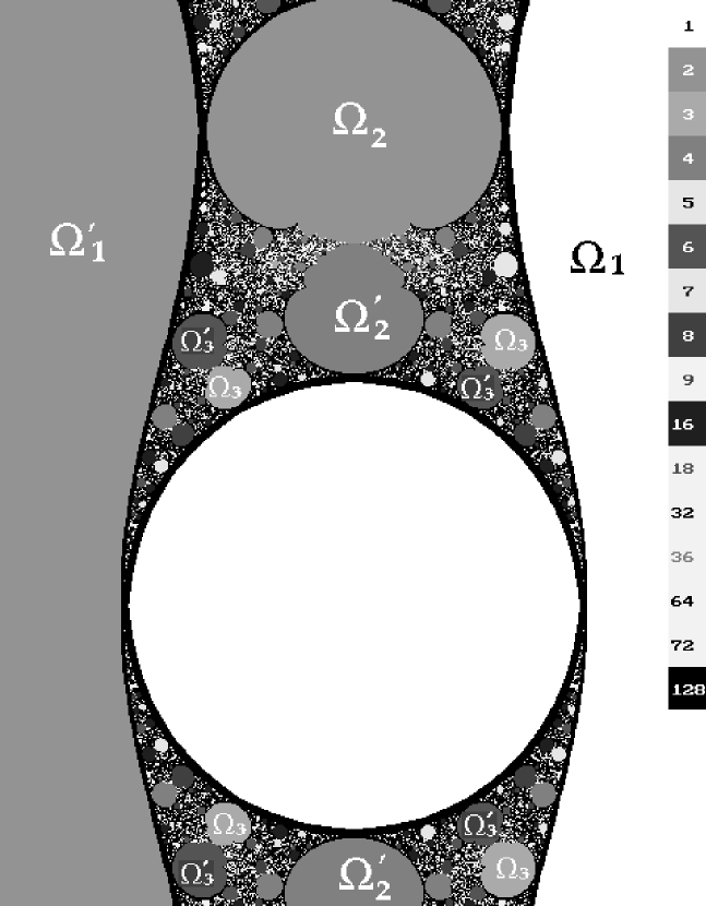
Figure 1: The parameter plane near the unit circle. The component pairs bud off the unit circle at the endpoints of rational internal rays.

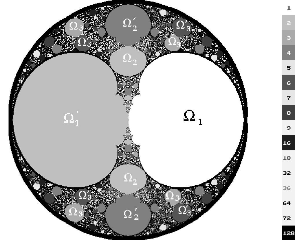
Figure 2: The parameter plane inverted by $\lambda\mapsto 1/\lambda$. The largest pair of components are the $\Omega_{1},\Omega_{2}$ of corollary 5.4.

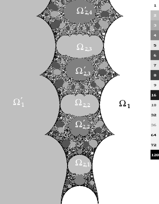
Figure 3: The $\lambda$ plane with the unit disk at the bottom of the figure. The component pairs $\Omega_{2,n},\Omega_{2,n}^{\prime}$ on the imaginary axis with virtual center at $(n+1/2)\pi$ are clearly visible.

8.1 The hyperbolic components

By corollary 7.2, it is clear that the period of all maps in a given component is the same. We therefore denote a generic hyperbolic component by $\Omega_{p}$ where $p$ is the period of the attracting cycle.

The following proposition is proved in [10].

Proposition 8.1

Suppose $\lambda\in{\mathbb{R}}$, $|\lambda|>1$. Then $J_{\lambda}={\mathbb{R}}$ and if $\lambda>1$, $f_{\lambda}$ has two attracting fixed points $z_{1}=it$ and $z_{2}=-it$ for some $t=t(\lambda)\in{\mathbb{R}}$, while if $\lambda<-1$, $(z_{1},z_{2})$ is an attracting cycle of period $2$.

Applying theorem 3.3 we obtain the corollary

Corollary 8.2

There is pair of components $(\Omega_{1},\Omega_{2})$ containing the positive and negative rays of the real axis with $|\lambda|>1$ respectively. For every $\lambda\in\Omega_{i},\,i=1,2$, $J_{\lambda}$ is a quasi-circle passing through $\infty$.

This pair of components can be characterized further by

Corollary 8.3

The component $\Omega_{1}$ containing the positive ray of the real axis, $\lambda>1$, is the unique hyperbolic component such that $f_{\lambda}$ has two distinct attracting fixed points; $\Omega_{2}$ containing the negative real ray is the unique component such that $f_{\lambda}$ has a single period two cycle attracting both asymptotic values. The boundary curve of $\Omega_{1}$ is asymptotic to the lines $t\pm ie^{|2t|}$ as $t=\Re\lambda\to\infty$ and the boundary curve of $\Omega_{2}$ is asymptotic to the lines $t\pm ie^{|2t|}$ as $t=\Re\lambda\to-\infty$.

Proof:   We need to show that if $|\lambda|>1$ and $f_{\lambda}$ has an attracting fixed point, then $\lambda\in\Omega_{1}$. Suppose $z=\lambda\tan z$ and $|\lambda\sec^{2}z|<1$. We can rewrite this condition as $|h(u)|=|u/\sin u|<1$ where $u=2z$. The locus $|h(u)|=1$ in the $u=x+iy$-plane consists of four branches, meeting at the origin and symmetric with respect to the origin. The branches are asymptotic to the lines $|x|\pm ie^{2|x|}$ as $|x|\to\infty$ and $|h(u)|<1$ in the upper and lower half regions. The function $T(u)=u/(2\tan 2u)$ satisfies $|T(u)|\leq 1$ in a bounded set. The complement of this set intersects the upper and lower half regions in two connected, simply connected unbounded domains. The function $\lambda=T(u)$ is even and maps each of these domains to a domain $\Omega$ in the $\lambda$ plane. It is clear that $\Omega$ must contain every $\lambda,|\lambda|>1$ for which $f_{\lambda}$ has an attracting fixed point. Moreover, $T$ maps the lines $x=0,y\neq 0$ to $\lambda>1$ so that $\Omega=\Omega_{1}$.

The asymptotic behavior of $\partial{\Omega_{1}}$ follows directly from that of the curves $|h(u)|=1$. By symmetry $\partial{\Omega_{2}}$ behaves the same way. $\;\square$

In the next three propositions we summarize the results on the properties of the remaining components of ${\cal H}$. We omit the proofs of propositions 8.4 and 8.5 since they are straightforward.

Proposition 8.4

Let $\Omega_{p}$ be a component of ${\cal H}-\Delta^{*}$ such that for $\lambda\in\Omega_{p}$ $f_{\lambda}$ has an attracting cycle of period $p$. Then either

• $f_{\lambda}$ has one attracting periodic cycle; both asymptotic values are in the immediate basin of the cycle and $p$ is even, or

• $f_{\lambda}$ has two attracting periodic cycles of period $p$; both cycles have the same multiplier; the cycles are symmetric with respect to the origin and a basin of each of them contains one of the asymptotic values.

Definitions: As usual, let $m_{\lambda}$ denote the multiplier of an attracting or neutral periodic cycle of $f_{\lambda}$ containing the point $z_{\lambda}$. If $\Omega_{p}$ is an arbitrary hyperbolic component of ${\cal H}$ and $\Delta^{*}$ is the unit disk punctured at the origin, the eigenvalue map $m:\Omega_{p}\rightarrow\Delta^{*}$is defined by $\lambda\mapsto m_{\lambda}$. For each $\alpha\in{\mathbb{R}}$ the internal ray $R(\alpha)$ is defined by $R(\alpha)=m^{-1}(re^{2\pi i\alpha}),0<r<1$.

Proposition 8.5

The eigenvalue map $m:\Delta^{*}\rightarrow\Delta^{*}$ is the identity. For each component $\Omega_{p}$ of ${\cal H}-\Delta^{*}$ the eigenvalue map is an infinite degree regular covering map.

The eigenvalue map lifts to a conformal isomorphism $\tilde{m}$ of $\Omega_{p}$ onto the upper half plane ${\mathbb{H}}$ defined by

$$\tilde{m}(\lambda)\mapsto 2\pi\arg{m(\lambda)}-i\log|m(\lambda)|$$

where the branch of the logarithm is chosen so that the internal ray $R(0)$ is mapped to $-i\log r$. Under this map the boundary of $\Omega_{p}$ corresponds to the real axis ${\mathbb{R}}$ and the common endpoint of all the internal rays of $\Omega_{p}$ is a boundary point that corresponds to the point at infinity under $\tilde{m}$.

Definition:  The boundary point corresponding to the point at infinity of the component $\Omega_{p}$ is called its virtual center. Recall that the hyperbolic components have no center since the functions in ${\cal F}$ have no critical points. The virtual center for the special components $\Omega_{1}$ and $\Omega_{2}$ above is $\infty$.

8.2 Virtual centers and component pairs

From now on we reserve the notation $\Omega_{p}$ for the components of ${\cal H}-\Delta^{*}$ with two distinct attracting cycles. We use $\Omega_{p}^{\prime}$ for the components with a single cycle of period $2p$. In particular, the component called $\Omega_{2}$ above is now renamed $\Omega_{1}^{\prime}$.

We will show that if $p>1$, the asymptotic values of the functions corresponding to the virtual centers of either $\Omega_{p}$ or $\Omega_{p}^{\prime}$ are prepoles of order $p-1$. For $p=1$, the common virtual center of $\Omega_{1}$ and $\Omega_{1}^{\prime}$ is infinity. The proof has two parts: we prove the statement first under the assumption that the components are bounded. We remove this assumption in the next section by describing the deployment of the $\Omega_{2}$ components.

Proposition 8.6

For any bounded hyperbolic component $\Omega_{p}$ or $\Omega_{p}^{\prime}$ with $p>1$, the virtual center $\lambda^{*}$ is finite and ${f^{\circ p-1}_{\lambda^{*}}}(\lambda^{*}i)=\infty$; that is $\lambda^{*}i$ is a prepole of order $p-1$.

Proof:   For $\lambda\in\Omega_{p}$, let $z_{0}=z_{0}(\lambda)$ be the attracting periodic point of $f_{\lambda}$ of period $p$ such that $z_{0}$ belongs to the component $D_{0}$ of the regular set that contains the asymptotic tract and such that $\lambda i$ and $z_{1}$ are both in $D_{1}=f(D_{0})$. Denote the preimage of $z_{0}$ in the periodic cycle by $z_{p-1}$ and the preimage of $D_{0}$ by $D_{p-1}$; then, for some $n$, $z_{p-1}=f^{-1}_{n}(z_{0})$. Since $p>1$, the domains $D_{p-1}$ and $D_{0}$ are different and the map $f:D_{p-1}\to D_{0}$ is bijective. Since $D_{0}$ contains the asymptotic tract and the map is bijective, there must be a unique pole, $s_{n}$, on $\partial{D_{p-1}}$. To see this, note that there is a preasymptotic tract at $s_{n}$ in $D_{p-1}$ containing a preimage of either $z=iy$ or $z=-iy$ for large $y>0$. So if $\partial{D_{p-1}}$ contained any other pole, there would be a preasymptotic tract in $D_{p-1}$ at this pole containing a preimage of the same segment and $f|_{D_{p-1}}$ would not be injective.

Since $\Omega_{p}$ is a component of the J-stable set, the Julia set and hence the prepoles vary continuously as we vary $\lambda$. Since the poles are fixed however, $s_{n}$ remains the unique pole on $\partial{D_{p-1}}$.

Suppose that $\lambda$ moves along the internal ray $R(\alpha)$ in $\Omega_{p}$ to the virtual center $\lambda^{*}$ as $r\rightarrow 0$, so that

$$\lim_{\lambda\stackrel{{\scriptstyle R}}{{\rightarrow}}\lambda^{*}}m_{\lambda}=0.$$

Since $(\tan z)^{\prime}=\sec^{2}z$, and $\lambda=z_{i}/\tan z_{i-1}$, the multiplier $m_{\lambda}$ can be written as

$$m_{\lambda}=[{f^{\circ p}_{\lambda}}(z_{0}({\lambda}))]^{\prime}=\Pi_{k=1}^{p}f^{\prime}_{\lambda}[{f^{\circ k-1}_{\lambda}}(z_{0}({\lambda}))]=\Pi_{k=1}^{p}2z_{i}/\sin 2z_{i-1}.$$

The only way some factor may tend to $0$ as $\lambda\to\lambda^{*}$ is for $\sin 2z_{i-1}\to\infty$ for some $i$, or equivalently, for $\Im z_{i-1}\to\infty$. Since $z_{0}$ is in the asymptotic tract, we conclude $\Im z_{0}\to\infty$.

By hypothesis $p>1$ and $\lambda^{*}\neq\infty$ so $z_{p-2}\neq z_{p-1}$. We have

$$\lim_{\lambda\stackrel{{\scriptstyle R}}{{\rightarrow}}\lambda^{*}}\lambda\tan z_{p-1}(\lambda)=\lim_{\lambda\stackrel{{\scriptstyle R}}{{\rightarrow}}\lambda^{*}}z_{0}=\infty.$$

We conclude further that $\lim_{\lambda\stackrel{{\scriptstyle R}}{{\rightarrow}}\lambda^{*}}z_{p-1}(\lambda)=\lim_{\lambda\stackrel{{\scriptstyle R}}{{\rightarrow}}\lambda^{*}}f^{-1}_{\lambda,n}(z_{0}(\lambda))=s_{n}$ and $\lim_{\lambda\stackrel{{\scriptstyle R}}{{\rightarrow}}\lambda^{*}}z_{1}(\lambda)=\lambda^{*}i$ so that $\lambda^{*}i$ is a prepole of of $f_{\lambda^{*}}$ of order $p-1$. The other periodic orbit behaves symmetrically and hence $-\lambda^{*}i$ is also a prepole.

If $\lambda\in\Omega_{p}^{\prime}$, $f_{\lambda}$ has a single cycle containing the points $z_{0}$ and $z_{p}=-z_{0}$. These lie in symmetric components $D_{0}$ and $D_{p}$ containing the asymptotic tracts. We argue as above that there are unique poles $s_{n}$ and $-s_{n}$ on their respective boundaries. If $\lambda^{*}$ is the virtual center, we again conclude that $\lim_{\lambda\stackrel{{\scriptstyle R}}{{\rightarrow}}\lambda^{*}}z_{1}(\lambda)=\lambda^{*}i$ and also that $\lim_{\lambda\stackrel{{\scriptstyle R}}{{\rightarrow}}\lambda^{*}}z_{p+1}(\lambda)=-\lambda^{*}i$ so that $\lambda^{*}i$ is a prepole of of $f_{\lambda^{*}}$ of order $p-1$. $\;\square$

The techniques developed by Douady, Hubbard and Sullivan for quadratic polynomials, showing that the boundary of a hyperbolic component is a piecewise analytic curve adapt easily to show that $\partial\Omega_{p}$ and $\partial\Omega_{p}^{\prime}$ are also piecewise analytic curves ([7, 9, 13]). The main difference is that the eigenvalue map is an infinite degree universal cover. Similarly, it is straightforward to modify the local techniques used to describe the root and bud structure of the Mandelbrot set ([13]). Note the following however: for $\lambda\in\Omega_{p}^{\prime}$, both $z_{0}$ and $-z_{0}$ belong to the attracting periodic cycle, $-z_{0}=f^{p}(z_{0})$ and $m_{\lambda}=\lambda^{2p}(\Pi_{i=0}^{p-1}\sec^{z}_{i})^{2}$. We thus redefine the map from the universal cover of $\Omega_{p}^{\prime}$ to the upper half plane ${\mathbb{H}}$ by $\tilde{m}\to 1/2(\arg m_{\lambda}-i\log|m_{\lambda}|)$. We omit the proofs of the following propositions (see [13]).

Proposition 8.7

Let $q>1$ and let $\lambda\in\partial\Omega_{p}$ be such that $m(\lambda)$ is a primitive $q$-th root of unity. Then there is a “bud” component $\Omega_{pq}$ with two attractive cycles of order $pq$ tangent to $\Omega_{p}$ at $\lambda$. Similarly, if $\lambda\in\partial\Omega_{p}^{\prime}$, and $m(\lambda)$ is a primitive $q$-th root of unity, there is either a bud component $\Omega_{pq}$ or a bud component $\Omega_{pq}^{\prime}$ attached at $\lambda$.

Proposition 8.8

At points of $\partial\Omega_{p}$ and $\partial\Omega_{p}^{\prime}$ such that $\tilde{m}(\lambda)=2\pi n$, $n\neq 0$, there is either a cusp or there may be a “root” component $\Omega_{d}$ where $d/p$. If $p=1$, the root component is $\Delta^{*}$. There are at most finitely many roots.

At a cusp of $\partial\Omega_{p}$, there are two cycles; at each point of each periodic cycle there is a single petal that contains the forward orbit of the asymptotic value attracted to that cycle. At a cusp of $\partial\Omega_{p}^{\prime}$ there is a single cycle; at each periodic point again there is a single petal, this time containing the forward orbits of both asymptotic values.

At a point of either $\Omega_{p}$ or $\Omega_{p}^{\prime}$ where a bud bifurcation of order $q>1$ occurs the points of the parabolic cycle always have $q$ petals. If the point is on $\Omega_{p}$ there are two cycles; at each parabolic periodic point there are $q$ petals and the forward orbit of the asymptotic value attracted to the cycle cycles through all the petals. If the bud point is on $\Omega_{p}^{\prime}$, there is a single cycle of period $2p$ and again at each point in the cycle there are $q$ petals. If the forward orbits of asymptotic values belong to distinct sets of petals, the bud component has two distinct attractive cycles of order $pq$, while if the forward orbits of asymptotic values belong to the same set of petals the bud component has a single cycle of period $2pq$. If the bud point is on $\Omega_{p}^{\prime}$, each petal contains the orbit of a different asymptotic value. On $\Omega_{p}^{\prime}$ there are bifurcation points with $q=1$; this happens if at each parabolic point there are two petals and the forward orbits of the asymptotic values are in different cycles of petals.

8.3 Components Tangent to $\Omega_{1}$ and $\Omega_{1}^{\prime}$

It follows from proposition 8.7 that there is a sequence $\lambda_{k}\in\partial\Omega_{1}$ with $\tilde{m}(\lambda_{k})=(2k+1)\pi$, $k\in{\mathbb{Z}}$ and a sequence of bud components $\Omega_{2,k}$ tangent to $\partial\Omega_{1}$ at $\lambda_{k}$. We know from theorem 5.2 and proposition 8.1 that $\Omega_{2,k}\cap{\mathbb{R}}=\emptyset$. Thus below we will fix $k$, set $\Omega_{2}=\Omega_{2,k}$ and assume that $\Im\lambda>0$ for $\lambda\in\Omega_{2,k}$.

We will prove that the virtual center of the component $\Omega_{2}=\Omega_{2,k}$ is $s_{k}i$ and so is finite; we will use this fact to conclude that, for all $p>1$, the components $\Omega_{p}$ and $\Omega_{p}^{\prime}$ are bounded. We need the following lemmas.

Lemma 8.9

Let $\Omega_{2}$ be a hyperbolic component such that for $\lambda\in\Omega_{2}$, $f_{\lambda}$ has two period two attracting cycles $z_{0},z_{1}$ and $-z_{0},-z_{1}$. If the virtual center $\lambda^{*}=\infty$, then for $j=0,1$, as $\lambda$ varies along some internal ray $R(\alpha)$ in $\Omega_{2}$,

$$\pm z^{*}_{j}=\lim_{\lambda\stackrel{{\scriptstyle R}}{{\rightarrow}}\lambda^{*}}(\pm z_{j}({\lambda}))=\infty.$$

Proof:   For $\lambda\in\Omega_{2}$ let $z_{0}=z_{0}(\lambda)$ belong to the component $D_{0}$ of the regular set that contains the asymptotic tract of $\lambda i$; then $\lambda i$ and $z_{1}$ are both in $D_{1}=f_{\lambda}(D_{0})$. The other periodic orbit $-z_{0},-z_{1}$ behaves symmetrically. Let us suppose that $\lambda$ moves along the internal ray $R(\alpha)$ in $\Omega_{2}$ to a limit point $\lambda^{*}=\infty$. Then $\lim_{\lambda\stackrel{{\scriptstyle R}}{{\rightarrow}}\lambda^{*}}m_{\lambda}=0$. It follows (compare the proof of proposition 8.6) that $\Im z_{0}(\lambda)\to+\infty$. We want to prove that $z^{*}_{1}=\lim_{\lambda\stackrel{{\scriptstyle R}}{{\rightarrow}}\lambda^{*}}z_{1}({\lambda})=\infty$. If not, there exists a sequence $\lambda_{n}\stackrel{{\scriptstyle R}}{{\rightarrow}}\lambda^{*}=\infty$, such that $\lim_{\lambda\stackrel{{\scriptstyle R}}{{\rightarrow}}\lambda^{*}}z_{1}({\lambda_{n}})=c\neq\infty$. Since $z_{1}(\lambda_{n})=\lambda_{n}\tan z_{0}(\lambda_{n})$, we must have $\lim_{\lambda_{n}\stackrel{{\scriptstyle R}}{{\rightarrow}}\lambda^{*}}\tan(z_{0}(\lambda_{n}))=0$. Thus either the curve $z_{0}(\lambda)$ is bounded and $\lim_{\lambda\stackrel{{\scriptstyle R}}{{\rightarrow}}\lambda^{*}}(z_{0}({\lambda}))=m\pi$ for some integer $m$, or the curve $z_{0}(\lambda)$ is unbounded but comes arbitrarily close to infinitely many integral multiples of $\pi$. Either possibility contradicts $\Im z_{0}(\lambda)\to\infty$. $\;\square$

Lemma 8.10

Let $\Omega_{2}$ be the bud component tangent to $\Omega_{1}$ at $\lambda_{k}$ as above. The virtual center $\lambda^{*}$ is equal to $s_{k}i$.

Proof:   We claim that $\lambda^{*}$ is finite. If not, by lemma 8.9, taking the limit along an internal ray, the periodic points $z_{0},z_{1}$ go to infinity, and in particular, $\Im z_{0}$ goes to infinity. We claim this cannot happen. For readability we suppress the dependence on $\lambda$ and on the ray; we set $\lambda=\lambda_{1}+i\lambda_{2}$, and $z_{j}=x_{j}+iy_{j}$, $j=0,1$. Since $z_{1}=\lambda\tan z_{0}$,

$$x_{1}=\frac{\lambda_{1}\sin(2x_{0})-\lambda_{2}\sinh(2y_{0})}{\cos(2x_{0})+\cosh(2y_{0})}.$$ (7)

and

$$y_{1}=\frac{\lambda_{1}\sinh(2y_{0})+\lambda_{2}\sin(2x_{0})}{\cos(2x_{0})+\cosh(2y_{0})}.$$ (8)

From lemma 8.9 we have $y_{0}\to\infty$ and by corollary 8.3 we have $\lambda_{2}\geq e^{|2\lambda_{1}|}$ and $\lambda_{2}\to\infty$. From equation 7 we see that $|x_{1}|\approx\pm\lambda_{2}\to\infty$. From the periodicity we obtain formulas for $x_{0}$ and $y_{0}$ by interchanging $0$ and $1$ in equations 7 and 8. Since $|x_{1}|\to\infty$ the term $\lambda_{2}\sin(2x_{1})$ in the equation for $y_{0}$ oscillates so $|\lambda_{1}\sinh(2y_{1})|$ must grow faster than $|\lambda_{2}\sin(2x_{1})|$; this implies $2y_{0}\approx\lambda_{1}\to\pm\infty$. The periodicity again implies $|x_{0}|\approx\pm\lambda_{2}\to\infty$ and $2y_{1}\approx\lambda_{1}\to\pm\infty$. To estimate the multiplier of the cycle we have

$$|\lambda\sec^{2}(z_{i})|\approx|\lambda_{2}|e^{\pm\lambda_{1}},$$

so that either

$$|m(\lambda)|=\lambda_{2}^{2}e^{\pm 2\lambda_{1}}\quad{\mbox{o}r}\quad|m(\lambda)|=\lambda_{2}^{2}.$$

Since the cycles of $f_{\lambda}$ are $(z_{0},z_{1})$ and $(-z_{0},-z_{1})$, the cycles of $f_{-\lambda}$ are $(z_{0},-z_{1})$ and $(z_{0},-z_{1})$ and we conclude that either $|m(\lambda)|$ or $|m(-\lambda)|$ grows with $\lambda_{2}^{2}$ and so cannot tend to zero.

Thus, $\lambda^{*}$ is finite and the asymptotic value of $f_{\lambda^{*}}$ must be a prepole of order 1 and so must be $s_{n}i$ for some pole $s_{n}$. We may draw a curve $\gamma_{k}$ in $\Omega_{2,k}$ from the bifurcation point $\lambda_{k}$ to the virtual center $s_{n}i$. These curves are disjoint and hence occur in order. We shall see in theorem 8.12 that each $s_{n}i$ is a virtual center of some component so the endpoint of $\gamma_{k}$ must be $s_{k}i$. $\;\square$

If $\lambda$ is the bifurcation point on $\partial\Omega_{1}$ for the bud $\Omega_{2}$, the point $-\bar{\lambda}$ is a bifurcation point on $\partial\Omega_{1}^{\prime}$ for a bud component $-\bar{\Omega}_{2}$. We leave it to the reader to check that the single period two cycle bifurcates to two period two cycles. The point here is that the forward orbits of the asymptotic values are in distinct cycles of petals at both bifurcation points.

Proposition 8.11

The hyperbolic components $\Omega_{p}$ and $\Omega_{p}^{\prime}$ are bounded for all $p>1$.

Proof:   For each integer $k$ we can draw the curves $\gamma_{k}$ and $-\bar{\gamma}_{k}$ in the components $\Omega_{2,k}$ and $-\bar{\Omega}_{2,k}$. Any hyperbolic component, not equal to $\Omega_{1},\Omega_{1}^{\prime},\Omega_{2,k}$ or $\bar{\Omega}_{2,k}$ must be contained inside a region bounded by curves $\gamma_{k},-\bar{\gamma}_{k},\bar{\gamma}_{k},-\gamma_{k}$ and arcs of $\partial\Omega_{1}$ and $\partial\Omega_{1}^{\prime}$. $\;\square$

8.4 Combinatorial invariants

If $\lambda^{*}$ is a virtual center, we know that $J_{\lambda^{*}}=\hat{\mathbb{C}}$, but the two sets

$$\{\infty,\pm\lambda^{*}i,f_{\lambda^{*}}(\pm\lambda^{*}i),\ldots,{f^{\circ p-2}_{\lambda^{*}}}(\pm\lambda^{*}i)\}$$

are cycles, considered as appropriate limits. They have a property that superattractive cycles have, namely, that each contains a singular value, the asymptotic value.

Set

$${\cal C}_{p}=\{\lambda:f^{p}_{\lambda}(\lambda i)=\infty\},\,\,{\cal C}=\cup_{1}^{\infty}{\cal C}_{p}.$$

The next theorem implies that if $\lambda\in{\cal C}_{p-1}$ there is a pair of components $(\Omega_{p},\Omega_{p}^{\prime})$ with $\lambda$ as virtual center. It follows that the itineraries of the virtual centers give a combinatorial description of the component pairs.

Theorem 8.12

Let ${\lambda}_{0}i$ be a prepole of order $p-1$ with ${f^{\circ p-2}}({\lambda}_{0}i)=s_{n}$. Then ${\lambda}_{0}$ is the virtual center of a component pair $(\Omega_{p},{\Omega}_{p}^{\prime})$ and $\lambda_{0}\in\partial{\Omega}_{p}\cap\partial{\Omega}_{p}^{\prime}$, where for $\lambda\in\Omega_{p},f_{\lambda}$ has two attracting cycles of period $p$ and for $\lambda\in\Omega_{p}^{\prime},f_{\lambda}$ has one attracting cycle of period $2p$.

Proof:   To prove this theorem, we need to show that there exist $\lambda$ and $\lambda^{\prime}$ arbitrarily close to $\lambda_{0}$ such that $f_{\lambda}$ has an attracting periodic cycle of period $p$ and $f_{\lambda^{\prime}}$ has an attracting periodic cycle of period $2p$. To construct the attracting periodic cycle we want to find $\lambda$ and a domain ${\mathbb{T}}$ in the dynamic plane such that ${f^{\circ p}}_{\lambda}({\mathbb{T}})\subset{\mathbb{T}}$.

For any choice of $r>0$ we can choose asymptotic tracts ${\cal A}^{+}=\{\Im z>r\}$ and ${\cal A}^{-}=\{\Im z<-r\}$ for $\pm\lambda_{0}i$ respectively. Since ${f^{\circ p-2}}(\lambda_{0}i)=s_{n}$, we have ${f^{\circ p-2}}(-\lambda_{0}i)=-s_{n}$. Set $U=f_{\lambda_{0}}({\cal A}^{+})$ so that $U$ is a neighborhood of $\lambda_{0}i$ and let $V$ be the corresponding neighborhood in the parameter plane; that is, $\lambda\in V$ if and only if $\lambda i\in U$.

For $\lambda\in V$ take the common preasymptotic tracts

$${\cal B}_{n}^{\pm}=\cap_{\lambda\in V}f^{-1}_{n,\lambda}({\cal A}^{\pm})$$

attached to the pole $s_{n}$. We can find $0<\delta=\delta(r)$ such that $|\arg(\lambda-\lambda_{0})|<\delta$ if $\lambda\in V$. Hence the angle between $f^{-1}_{n,\lambda}({\mathbb{R}})$ and ${\mathbb{R}}$ at $s_{n}$ is bounded and ${\cal B}^{\pm}$ contains some triangular domain with one vertex at $s_{n}$. Define a map $g:V\rightarrow{\mathbb{C}}$ by $g(\lambda)={f^{\circ p-2}_{\lambda}}(\lambda i)$ for $\lambda\in V$. Then $g(V)$ is an open set containing the pole $s_{n}$ and there exist open sets $V^{\pm}\subset V$ such that $V^{\pm}=g^{-1}({\cal B}_{n}^{\pm})$. For any $\lambda\in V^{+}$, ${f^{\circ p-1}_{\lambda}}(\lambda i)$ belongs to an asymptotic tract ${\cal A}^{+}=\{\Im z>r^{\prime}\}$ where possibly $r^{\prime}<r$. Moreover, for inverse branches such that

$${f^{\circ-(p-2)}_{{\bf n}_{p-2},\lambda_{0}}}(s_{n})=\lambda_{0}i,$$

we have the property that $v_{\lambda}={f^{\circ-(p-2)}_{{\bf n}_{p-2},\lambda}}(s_{n})\neq\lambda i$, so that there are preimages $w_{k,\lambda}=f^{-1}_{k,\lambda}(v_{\lambda})$ in the upper half of each strip $L_{k},k\in\bf Z$. These $w_{k,\lambda}$ depend continuously on $\lambda$ and if $\lambda\rightarrow\lambda_{0}$, then $\Im w_{k,\lambda}\rightarrow\infty$.

Let $\eta_{\lambda}=|\lambda i-v_{\lambda}|$ and consider the ball $B_{\lambda}=B(v_{\lambda},\eta_{\lambda})$. Then ${f^{\circ p-2}_{\lambda}}(B_{\lambda})$ is an open set containing $s_{n}$. Using the principal part of $f_{\lambda}$ we see that ${f^{\circ p-1}_{\lambda}}(B_{\lambda})=\hat{\mathbb{C}}-B(0,R_{\lambda})$ where $R_{\lambda}\approx|{f^{\circ p-1}_{\lambda}}(\lambda i)|$ and $R_{\lambda}\to\infty$ as $\lambda\to\lambda_{0}$. We claim that $\Im{f^{\circ p-1}_{\lambda}}(\lambda i)>\Im w_{k,\lambda}$. Let

$$K=\max_{z\in\bar{U},\lambda\in\bar{V}}|({f^{\circ p-2}_{\lambda}})^{\prime}(z)|.$$

Since $|\lambda|>1$ and $|\lambda|\gg\eta_{\lambda}$, we argue as in the proof of proposition  6.3 and obtain

$$\Im w_{k,\lambda}=\Im f_{\lambda}^{-1}(v_{\lambda})=\Im f_{\lambda}^{-1}(\lambda i+\eta_{\lambda})=\Im\left[\frac{1}{2i}\log\frac{i\eta_{\lambda}}{2\lambda-i\eta_{\lambda}}\right].$$

Thus, $\Im w_{k,\lambda}\approx\frac{1}{2}|\log|\eta_{\lambda}||$.

Now set $y_{0}=\frac{1}{2}|\log\eta_{\lambda}|$. Then $|f^{-1}_{n,\lambda}(iy_{0})-s_{n}|\approx 2\lambda/|\log\eta_{\lambda}|$ and consequently

$$|{f^{\circ-(p-1)}_{{\bf n}_{p-1},\lambda}}(iy_{0})-\lambda i|\geq|f^{-1}_{n,\lambda}(iy_{0})-s_{n}|\cdot\min_{w\in{f^{\circ p-2}_{\lambda}}(U)}|({f^{\circ-(p-2)}_{{\bf n}_{p-2},\lambda}})^{\prime}(w)|$$

and approximating,

$$|{f^{\circ-(p-1)}_{{\bf n}_{p-1},\lambda}}(iy_{0})-\lambda i|\geq{2\lambda\over{K|\log\eta_{\lambda}|}}.$$

But $|\lambda i-v_{\lambda}|=\eta_{\lambda}$ and since $\eta_{\lambda}$ is assumed small

$$\frac{2\lambda}{K|\log\eta_{\lambda}|}\geq\eta_{\lambda}.$$

Therefore

$$|{f^{\circ p-2}_{\lambda}}(\lambda i)-s_{n}|\leq|f^{-1}_{n,\lambda}(iy_{0})-s_{n}|$$

so that

$$\Im{f^{\circ p-1}}_{\lambda}(\lambda i)>iy_{0}$$

and

$$\Im{f^{\circ p-1}_{\lambda}}(\lambda i)>\Im w_{k,\lambda}\approx y_{0}$$

as claimed.

Now we are ready to construct the domain ${\mathbb{T}}$ inside an asymptotic tract ${\cal A}^{+}$ for some $\lambda$ in $V$ with ${f^{\circ p}_{\lambda}}({\mathbb{T}})\subset{\mathbb{T}}$ proving that $\lambda\in\Omega_{p}$. Set $r=r_{\lambda}=(1/2)|\log\eta_{\lambda}|-\epsilon$, and choose an asymptotic tract ${\cal A}^{+}=\{z:\Im z>r_{\lambda}\}$ so that $v_{\lambda}\in f_{\lambda}({\cal A}^{+})$. Let $I^{\pm}$ be two rays meeting at $s_{n}$ such that the triangular domain $T$ between them containing the vertical direction is contained in $f^{-1}_{n,\lambda}({\cal A}^{+})$ and such that ${f^{\circ p-2}_{\lambda}}(\lambda i)\in T$. Let $\cal T$ be the triangular region with vertex at $v_{\lambda}$ bounded by ${\cal I}^{\pm}=f^{-(p-2)}_{{\bf n}_{p-2},\lambda}(I^{\pm})$ and an arc of the boundary of $f_{\lambda}({\cal A}^{+})$ so that $\lambda i\in\cal T$. Finally, set ${\mathbb{T}}=\cup_{k\in{\mathbb{Z}}}f^{-1}_{k,\lambda}(\cal T)$. Then ${\mathbb{T}}$ is an asymptotic tract whose “horizontal” boundary is scalloped by preimages of $\partial\cal T$; that is, it is made up of arcs $f^{-1}_{k,\lambda}({\cal I}^{\pm})$ that meet at $w_{k,\lambda}$ and are joined by intervals in the line $y=r_{\lambda}$.

Now consider $\tilde{\mathbb{T}}={f^{\circ p-1}_{\lambda}}(\cal T)$; this is a triangle with a vertex at infinity; the sides meeting there are rays and the third side is an arc of a circle centered at the origin with radius slightly smaller than $|{f^{\circ p-1}_{\lambda}}(\lambda i)|$. Because $|{f^{\circ p-1}_{\lambda}}(\lambda i)|>(1/2)|\log\eta_{\lambda}|$, we may assume $|\partial{{f^{\circ p}_{\lambda}}({\cal A}^{+})}|>(1/2)|\log\eta_{\lambda}|$ for small $\epsilon$. To claim that ${f^{\circ p}_{\lambda}}({\mathbb{T}})\subset{\mathbb{T}}$ we need to check two conditions:

1. $\Im{f^{\circ p-1}_{\lambda}}(\lambda i)>r_{\lambda}$ and

2. $f_{\lambda}(I^{\pm})\subset{\cal A}^{+}$.

Now $\lambda$ was chosen so that ${f^{\circ p-1}_{\lambda}}(\lambda i)$ belongs to its asymptotic tract hence changing the argument of $\lambda$ if necessary we can insure that 1. holds. We can insure 2. by decreasing the angle between $I^{\pm}$ if necessary.

In the above we chose $\lambda\in V^{+}$ such that ${f^{\circ p-2}_{\lambda}}(\lambda i)\in{\cal B}^{+}$. Next we show that if $\lambda\in V^{-}$ and ${f^{\circ p-2}_{\lambda}}(\lambda i)\in{\cal B}^{-}$ then $\lambda\in\Omega_{2p}$. Take inverse branches such that

$${f^{\circ-(p-2)}_{{\bf n}_{p-2},\lambda_{0}}}(s_{n})=\lambda_{0}i\mbox{ and }{f^{\circ-(p-2)}_{{\bf n}_{p-2},\lambda_{0}}}(-s_{n})=-\lambda_{0}i.$$

Since ${f^{\circ p-2}_{\lambda}}(\lambda i)\in{\cal B}^{-}$ we have ${f^{\circ p-1}_{\lambda}}(\lambda i)\in{\cal A}^{-}.$ Now ${f^{\circ p}_{\lambda}}(-\lambda i)\in{\cal B}^{+}$ so ${f^{\circ 2p-1}_{\lambda}}(\lambda i)\in{\cal A}^{+}$. Therefore, arguing analogously to the above we can prove that $\lambda\in\Omega_{p}^{\prime}$. $\;\square$

The following corollaries are immediate.

Corollary 8.13

Assume $p\geq 2$ and $\lambda\in\Omega_{p}\cup\Omega_{p}^{\prime}$.

• if the asymptotic value $\lambda i$ is contained in the preasymptotic tract ${\cal B}_{v}^{+}$ of the prepole $v$ of order $p-1$ (respectively $-\lambda i\in{\cal B}_{v}^{-}$), then $f_{\lambda}$ has two attracting periodic cycles of period $p$ and $\lambda\in\Omega_{p}$.

• if the asymptotic value $\lambda i$ is contained in the preasymptotic tract ${\cal B}_{v}^{-}$, then there is a single periodic cycle of period $2p$ attracting both singular values and $\lambda\in\Omega_{p}^{\prime}$ .

Corollary 8.14

Let $(\Omega_{p},\Omega_{p}^{\prime})$ be a pair of hyperbolic components meeting at the virtual center $\lambda^{*}$. Suppose $\lambda(t),\,t\in[0,1]$ is a curve in the parameter plane passing from $\Omega_{p}$ to $\Omega_{p}^{\prime}$ through $\lambda^{*}$. Then there is a period doubling bifurcation of attracting periodic points of $f_{\lambda}$.

8.5 Duality of the virtual centers and prepoles

In this section we show that the virtual centers in the parameter plane play a role that is dual to the prepoles in the dynamic plane.

Proposition 8.15

Let $\lambda_{n}\in{\cal C}_{p-1}$ where ${f^{\circ p-2}_{\lambda_{n}}}(\lambda_{n}i)=s_{n}$; that is, $\lambda_{n}$ is the virtual center of a component pair $(\Omega_{p},\Omega_{p}^{\prime})$. Then there is a sequence of component pairs $(\Omega_{p+1,k},\Omega_{p+1,k}^{\prime}),\;k\in{\mathbb{Z}}$, with centers $\lambda_{k}\in{\cal C}_{p}$ where ${f^{\circ p-1}_{\lambda_{k}}}(\lambda_{k}i)=s_{k}$ and $\lambda_{k}\rightarrow\lambda_{n}$ as $|s_{k}|\rightarrow\infty$.

Proof:   Let $B(\lambda_{n}i,\epsilon)$ be an $\epsilon$ neighborhood of the asymptotic value $\lambda i$ of $f_{\lambda}$ in the dynamic plane. Let $D(\lambda_{n},\epsilon)$ be the corresponding neighborhood in the parameter plane. By assumption ${f^{\circ p-2}_{\lambda_{n}}}(\lambda_{n}i)=s_{n}$. Define a map $g:D(\lambda_{n},\epsilon)\rightarrow\hat{\mathbb{C}}$ by $g(\lambda)={f^{\circ p-1}_{\lambda}}(\lambda i)$. Then $g(D(\lambda_{n},\epsilon))$ is a neighborhood of infinity. Therefore, for large $k$, there is a parameter $\lambda_{k}\in D(\lambda_{n},\epsilon)$ such that

$$g({\lambda}_{k})={f^{\circ p-1}_{\lambda_{k}}}(\lambda_{k}i)=s_{k}.$$

Thus $\lambda_{k}\in{\cal C}_{p}$ and by theorem  8.12 $\lambda_{k}$ is the virtual center of a component pair $(\Omega_{p+1,k},\Omega_{p+1,k}^{\prime})$; moreover, $\lambda_{k}\rightarrow\lambda_{n}$ as $|s_{k}|\rightarrow\infty$. $\;\square$

Proposition 8.16

The accumulation points of ${{\cal C}}_{p}$ are parameters belonging to $\cup^{p-1}_{k=1}{{\cal C}}_{k}\cup\{\infty\}$. For $p\geq 1$, let ${\lambda}_{n}\in{{\cal C}}_{p},\,n\in{\mathbb{Z}},$ be a sequence of virtual centers with itineraries ${\bf n}_{p}=(n_{1},n_{2},\ldots,n_{p})$.

• if the entries $n_{i},i=1,2,\ldots,p-1$ are the same for all ${\lambda}_{n}$ and $n_{p}=n,$ then the accumulation point of ${\lambda}_{n}$ belongs to ${{\cal C}}_{0}=\{\infty\}$ and

• if the entries $n_{i},i=2,\ldots,p$ are the same for all ${\lambda}_{n}$ and $n_{1}=n$, then the accumulation point of ${\lambda}_{n}$ is a virtual center ${\lambda}\in{{\cal C}}_{p-1}$ with itinerary ${\bf n}_{p-1}=(n_{2},\ldots,n_{p})$; that is, $f^{p-2}_{\lambda}(\lambda i)=s_{n_{2}}$.

Proof:   Consider the map $g:{\mathbb{C}}-\cup^{p-1}_{k=1}{{\cal C}}_{k}\to\hat{{\mathbb{C}}}$ defined by $g({\lambda})=f^{p}_{\lambda}(\lambda i).$ The map $g$ is not defined at the points $\lambda\in\cup^{p-1}_{k=1}{{\cal C}}_{k}$ since these points are essential singularities of $g$; $g$ has poles at $\lambda\in{{\cal C}}_{p}$ and is holomorphic otherwise. Let $\lambda={\lim}_{n\to\infty}(\lambda_{n}),\,\lambda_{n}\in{{\cal C}}_{p}$. If $\lambda\notin\cup^{p-1}_{k=1}{{\cal C}}_{k}\cup\{\infty\}$ then $g(\lambda)$ is well-defined and holomorphic in a neighborhood of $\lambda$. On the other hand $\lambda$ is an accumulation point of poles and so $g$ has a non-removable singularity at $\lambda$. Thus we arrive at contradiction.

The proof of the second part of the proposition is the same as the proof of proposition  6.1, since the itineraries of the virtual centers are defined by the itineraries of the corresponding prepoles. $\;\square$

Corollary 8.17

If $\lambda\in{\mathbb{C}}-{{\cal C}}$ then for each $p\in{\mathbb{N}}$, there is a neighborhood $U$ of $\lambda$ such that

$$U\cap\left(\cup^{p-1}_{k=1}{{\cal C}}_{k}\right)=\emptyset.$$

9 Deformation of cycles

We have seen that the periodic points and their multipliers are holomorphic functions of the parameter $\lambda$, defined by a holomorphic motion, in any hyperbolic component of the parameter space. We could also obtain these functions by analytic continuation of local solutions to the functional equations ${f^{\circ p}_{\lambda}}(z)=z$ for all positive integers $p$. At a boundary point of the hyperbolic component, some of these local solutions may still have analytic continuations while others do not.

Let $\lambda(t),\,t\in[0,1]$ be a path defined in the parameter plane $X$ with $\lambda(0)=\lambda_{0}$ and $\lambda(1)=\lambda^{*}\neq\infty$. For a given cycle, $\{z_{i}\}_{i=0}^{p-1}$, assume that we have a path in $X\times{\bf C}$ defined by analytic continuation of function elements of the functional equation, $z_{i}(t)=z_{i}(\lambda(t))$, $t\in[0,1)$. Denote the multiplier function for the cycle by $m(t)=m(\lambda(t))$.

If $\lim_{t\to 1}m(t)=1$, the functions $z_{i}(t)$ cannot be analytically continued to $\lambda^{*}$ and $\lambda^{*}$ is called an algebraic singularity in analogy with the rational map case. Note that this limit is independent of the path. If, however, for some path, $\lambda(t)\to\lambda^{*}$, $\lim_{t\to 1}m(t)=\infty$ or doesn’t exist, then $\lambda^{*}$ is called a transcendental singularity for the cycle $z(t)$.

Next we show that a transcendental singularity $\lambda^{*}$ of a periodic cycle of period $p$ is a special point on the boundary of a hyperbolic component; it is, in fact, the virtual center of a pair hyperbolic pair, $\Omega_{p},\Omega_{p}^{\prime}$. This, together with theorem 8.12 shows that there is a one to one correspondence between the transcendental singularities of the periodic points and the virtual centers of the hyperbolic component pairs.

Lemma 9.1

Suppose $\lambda^{*}$ is a transcendental singularity for the cycle $z(t)$. Then, each of the curves $z_{i}(t)$, $i=0,\ldots,p-1,\,t\in[0,1)$ has a limit point, perhaps infinite, in $(\lambda^{*},\hat{\mathbb{C}})$, the dynamic plane of $f_{\lambda^{*}}$.

Proof:   Let $A$ be the accumulation set of $\{z_{p-1}(t)\}$ in $(\lambda^{*},\hat{\mathbb{C}})$. If $A$ is not a point, then $A$ is a continuum. We claim it cannot be a continuum.

Let $w\neq\infty\in A$ and let $t_{n}\to 1$ be such that $z_{p-1}(t_{n})\to w$. Because of the functional relation, $z_{p-1}(t_{n})={f^{\circ p}}(z_{p-1}(t_{n}))$. As we let $n\to\infty$, either we have $w={f^{\circ p}_{\lambda^{*}}}(w)$ and $\lambda^{*}$ is not a transcendental singularity or ${f^{\circ p}_{\lambda^{*}}}(w)$ is not defined and $w$ is a prepole or $f_{\lambda^{*}}$ of order at most $p$. Since there are only countably many prepoles of order at most $p$, they form a discrete set and $A$ is not a continuum. The same is true for each path $z_{i}(t),\,i=1\ldots,p-1$. Assume therefore that the endpoint $z_{0}(1)$ is a prepole so that some $z_{k}(t)$ is unbounded. We shall see below that only one curve can be unbounded if the cycle is not symmetric and that two curves are unbounded if it is symmetric. For definiteness, we shall always assume the points are ordered so that $z_{p-1}(t)$ is unbounded. $\;\square$

Proposition 9.2

If the periodic point $z(\lambda)$ has a transcendental singularity at $\lambda^{*}$ then there exists a hyperbolic component $\Omega_{p}$ (or $\Omega_{p}^{\prime}$) with virtual center at $\lambda^{*}\in{\cal C}_{p-1}$ and $\lambda(t)\in\Omega_{p}$ (resp. $\Omega_{p}^{\prime}$) for $t>t_{0}$.

Proof:   Since we will only be interested in the situation where $p$ is large, we omit the discussion of the special but not too difficult exceptional cases $p\leq 2$ and assume $p>2$.

By assumption there is a path $\lambda(t)\to\lambda^{*},t\in[0,1]$ in the parameter plane such that the branch $z_{p-1}(t)\to\infty$ as $t\to 1$. First we prove that the limit $z_{p-2}(1)$ is some pole $s_{n}$. We know

$$\lim_{t\to 1}z_{p-1}(t)=\lim_{t\to 1}\lambda(t)\tan z_{p-2}(t)=\infty,$$

$\lambda(t),\,t\in[0,1]$ is bounded and $\lim z_{p-2}(t)$ is a point in ${\mathbb{C}}$. This implies that

$$\lim_{t\to 1}\tan z_{p-2}(t)=\infty$$

and that the endpoint of the curve is a pole $s_{n}$; that is,

$$\lim_{t\to 1}z_{p-2}(t)=\lim_{t\to 1}f^{-1}_{n,t}(z_{p-1}(t))=s_{n}.$$

Note that the closed curve $z_{p-2}(t)$ is bounded and has ends $z_{p-2}(0)$ and $z_{p-2}(1)=s_{n}$. It cannot intersect the curve $\lambda(t)i$ except at the endpoint $\lambda^{*}i$ because all points in $z_{p-2}(t)$ are images of points in $z_{p-3}(t)$ and $\lambda(t)i$ is omitted for $f_{t}$.

We now show that the endpoint of one of the branches is an asymptotic value. To do this we need to find an asymptotic path in the dynamic plane of $f_{\lambda^{*}}$. Draw the projections of the branch curves $z_{i}(t)$ to this plane and use the same notation for them. Now let $\beta(t)={f^{\circ p}_{\lambda^{*}}}(z_{p-2}(t))$. Initially, $\beta$ and $z_{p-2}$ may be far apart, but since $f_{\lambda}(z)$ is holomorphic in both $\lambda$ and $z$, and since both paths end at the pole $s_{n}$, given $\eta$ there is a $t_{0}$ such that for $t>t_{0}$,

$$|\beta(t)-z_{p-2}(t)|=|{f^{\circ p}_{\lambda^{*}}}(z_{p-2}(t))-{f^{\circ p}_{\lambda}}(z_{p-2}(t))|<\eta.$$ (9)

Now set $\alpha(t)=f_{\lambda^{*}}(\beta(t))$. Since $\lim_{t\to 1}\beta(t)$ is a pole, $\alpha(t)$ is unbounded. The curve $z_{p-2}(t)$ is bounded and we shall assume for the moment for simplicity, that all the curves $z_{i}(t)$, $i=0,\ldots,p-2$ are bounded — we shall eliminate this assumption at the end of the proof. Because the preimage of a closed bounded set under a tangent map is unbounded if and only if the bounded set contains an asymptotic value, $f_{\lambda^{*}}(z_{p-1}(t))$ ends at an asymptotic value and thus so does $z_{0}(t)$; furthermore, both $\alpha(t)$ and $z_{p-1}(t)$ are asymptotic paths; to wit, $\Im z_{p-1}(t)\to\infty$. Thus, ${f^{\circ p-2}_{\lambda^{*}}}(\lambda^{*}i)=\pm s_{n}$ and by symmetry both $\lambda^{*}$ and $-\lambda^{*}$ are virtual centers.

Using the map $f_{\lambda^{*}}$ and the itinerary of the cycle, the $i$-th preimage of the curve $\alpha(t)$ has the same limit as $t\to 1$ as the curve $z_{p-1-i}(t)$, $i=1,\ldots,p-1$.

Next we need to prove that $\Re z_{p-1}(t)$ stays bounded. The argument is reminiscent of the proof that there are no Herman rings for these functions. It isn’t the same, however, because now parameter values vary. We therefore use the same trick as we did above; we use the curve $\alpha(t)$ and work in the dynamic plane of $f_{\lambda^{*}}$. Then, if we assume $\Re z_{p-1}(t)$ is unbounded, $\Re\alpha(t)$ is also unbounded. It follows that the range of $\arg(f_{\lambda^{*}}(\alpha(t))-\lambda^{*}i)$ contains either a semi-infinite interval $(\theta,\infty)$ or a union of semi-intervals $(\theta_{k},\theta_{k+1}),\,k\to\infty$. Let $U$ be a neighborhood of $\lambda^{*}i$ and let $I$ be any straight line through $\lambda^{*}i$. Then $f_{\lambda^{*}}(\alpha(t))$ meets $I$ infinitely often on both sides of $\lambda^{*}i$.

Now for $r\gg 0$, $J=f_{n,\lambda^{*}}^{-1}((-\infty,r)\cup(r,\infty))$ is a curve containing $s_{n}$ in its interior. Since $f_{\lambda^{*}}^{p-2}(U)$ contains a neighborhood of $s_{n}$, the curve $f_{\bf n_{p-2},\lambda^{*}}^{-(p-2)}(J)$ intersects $f_{\lambda^{*}}(\alpha(t)$ infinitely often on both sides of $\lambda^{*}i$ and hence there is a sequence $t_{n}$, $n\to\infty$ such that $f_{\lambda^{*}}^{p-1}(\alpha(t_{n}))\cap J\neq\emptyset$ and $f_{\lambda^{*}}^{p}(\alpha(t_{n}))\in{{\mathbb{R}}}$. This contradicts equation (9) and the fact that $\Im z_{p-1}(t)\to\infty$. We conclude not only that $\Re z_{p-1}(t)$ stays bounded, but that for $t$ close to $1$, it must stay inside a strip of width $\pi$.

To show that the path $\lambda(t)$ enters a hyperbolic component we prove

$$\lim_{t\to 1}\left|\prod^{p-1}_{i=0}f^{\prime}_{t}(z_{i}(t))\right|=0$$

where, as usual, $f_{t}=f_{\lambda(t)}$. We have

$$|f^{\prime}_{t}(z_{p-2}(t))|=\left|\lambda(t)\left(1+{z^{2}_{p-1}(t)}/{\lambda^{2}(t)}\right)\right|\approx{\rm O}(|\lambda(t)|^{-1}|z^{2}_{p-1}(t)|)$$ (10)

and

$$\left|f^{\prime}_{t}(z_{p-1}(t))\right|=|{\lambda}(t)||\sec^{2}(z_{p-1}(t))|=4|{\lambda}(t)|\left|(e^{iz_{p-1}(t)}+e^{-iz_{p-1}(t)})^{-2}\right|.$$ (11)

Since $|\lambda(t)|<K$ for some $K>0$ and $\Im z_{p-1}(t)\to\infty$ as $t\rightarrow 1$,

$$|\sec^{2}(z_{p-1}(t))|={\rm O}\left(|{\lambda}(t)|e^{-2\Im z_{p-1}(t)}\right)\rightarrow 0$$ (12)

By equations (10)— (12), as $t\to 1$,

$$|\sec^{2}z_{p-2}(t)\sec^{2}z_{p-1}(t))|={\rm O}(|z_{p-1}(t)|^{2}e^{-2\Im z_{p-1}(t)}).$$

Because $\Re z_{p-1}(t)$ is universally bounded for $t\to 1$ , while $\Im z_{p-1}(t)\to\infty$,

$$|z_{p-1}^{2}(t)|e^{-2\Im z_{p-1}(t)}\to 0.$$

By assumption, the curves $z_{i}(t),\,i=0,\ldots,p-2$ stay a positive distance from all poles (at least for $t$ close to 1), so there exists a bound $C>0$ such that

$$\left|\prod^{p-3}_{i=0}f^{\prime}_{t}(z_{i}(t))\right|\leq C.$$

Then

$$|m(t)|={\rm O}(\Im z^{2}_{p-1}(t)e^{-2\Im z_{0}(t)})\to 0$$

so there is some $t^{\prime}\in[0,1)$ such that the multiplier

$$|m(t)|=\left|\prod^{p-1}_{i=0}f^{\prime}_{t}(z_{i}(t))\right|<1$$

for $t>t^{\prime}$; $z_{i}(t^{\prime}),i=0,\ldots,p-1$ is a neutral periodic cycle. Thus for $t>t^{\prime},\,\lambda(t)$ belongs to some hyperbolic component ${\Omega}_{p}$ of ${\cal H}^{0}$ and $\lambda^{*}=\lim_{t\to 1}\lambda(t)$ is a virtual center of ${\Omega}_{p}$.

Now suppose there is a branch $z_{i}(t)\neq z_{p-1}(t)$ such that $\lim_{t\to 1}z_{i}(t)=\infty$. Arguing as above, $z_{i-1}$ tends to a pole and $z_{i+1}$ tends to an asymptotic value. Since there are only two asymptotic values, either the cycle is symmetric and contains both asymptotic values or it has a lower period $q|p$. Again since $\Re z_{i}(t)$ is bounded, $\sec^{2}z_{i-1}(t)\sec^{2}z_{i}(t)\to 0$ and for all branches $z_{j}(t)$ such that $z_{j}(1)$ is not a pole or $z_{j}(1)\neq\infty$, there is a constant independent of $t$ and $j$ such that $|\sec^{2}z_{j}(t)|<C$; thus, as $t\to 1$ the periodic cycle becomes an attractive cycle of the same period.

Finally, from the proof of theorem 8.12, we conclude either $f_{t}$ has a distinct symmetric cycle $-z_{i}(t),i=0,\ldots,p-1$ and that $q=p$, or the cycle $z_{i}(t),i=0,\dots,p-1$ is symmetric with respect to the origin, $q=p/2$ and $\lambda\in\Omega_{p^{\prime}}$ with virtual center at $\lambda^{*}$. $\;\square$

We close this discussion by considering the behavior of a periodic cycle and its multiplier, in and on the boundary of the hyperbolic component where it is the attracting cycle.

Proposition 9.3

Let $\lambda^{*}$ be the virtual center of the component pair $(\Omega_{p},\Omega_{p}^{\prime}).$ If $z_{0}(\lambda),z_{1}(\lambda),\ldots,z_{p-1}(\lambda)$ is an attracting periodic cycle of period $p$ for $\lambda\in\Omega_{p}$, and if $m_{\lambda}$ is its multiplier, then

1. $z_{i}(\lambda)$ and $m_{\lambda}$ are transcendental meromorphic functions of $\lambda$;
   $m_{\lambda}$ has an essential singularity at $\lambda^{*}$ as does $z_{\lambda}=z_{k}(\lambda)$ for some $k\in\{0,\ldots,p-1\}$.

2. $\lambda^{*}i$ is an asymptotic value of $f_{\lambda^{*}}=z_{k+1}(\lambda^{*})$, $0$ is an asymptotic value of $m_{\lambda}$ and $\Omega_{p}$ is an asymptotic tract for both $m_{\lambda}$ and $z_{k+1}(\lambda)$.

3. $z_{\lambda}$ has algebraic singularities at a sequence of points $\lambda_{j}\in\partial{\Omega}_{p}$ where $m(z_{\lambda_{j}})=1$ and $\lambda_{j}\to\lambda^{*}$ as $j\to\infty$.

Proof:   By proposition 9.2, if $\lambda\to\lambda^{*}$ inside $\Omega_{p}$, then for some $k$, $\Im z_{k}(\lambda)\rightarrow\infty$ and $f_{\lambda}(z_{k}(\lambda))\rightarrow\lambda^{*}i$. Relabelling the cycle if necessary we may assume $k=p-1$ so that $z_{0}(\lambda)\rightarrow\lambda^{*}i$. Now set $z_{\lambda}=z_{0}(\lambda)$. Because $\lambda^{*}i$ is a prepole of $f_{{\lambda}^{*}}$ of order $p-1$, ${f^{\circ p}_{\lambda^{*}}}(\lambda^{*}i)$ is not defined and so neither is $m_{\lambda}$, proving 1.

To prove 2. note that the equation ${f^{\circ p}_{\lambda}}(z_{\lambda})=z_{\lambda}$ has no solution for $\lambda=\lambda^{*}$ and that ${\lambda}^{*}i$ is an asymptotic value of $z_{\lambda}$. Because $\lambda^{*}$ is a virtual center of ${\Omega}_{p},$ we see from proposition  8.5 that if $\lambda\to{\lambda^{*}}$ inside ${\Omega}_{p}$ then $m_{\lambda}\rightarrow 0$.

The third point follows from propositions  8.5 and  9.2. $\;\square$

References

• [1] L. Ahlfors and L. Bers. Riemann’s mapping theorem for variable metrics. Annals of Math., 72:385–404, 1960.
• [2] I.N. Baker, J.Kotus, and Y.Lü. Iterates of meromorphic functions ii: Examples of wandering domains. J. London Math. Soc., 42(2):267–278, 1990.
• [3] I.N. Baker, J.Kotus, and Y.Lü. Iterates of meromorphic functions i. J. Ergodic Th. and Dyn. Sys., 11:241–248, 1991.
• [4] I.N. Baker, J.Kotus, and Y.Lü. Iterates of meromorphic functions iii: Preperiodic domains. J. Ergodic Th. and Dyn. Sys., 11:603–618, 1991.
• [5] I.N. Baker, J.Kotus, and Y.Lü. Iterates of meromorphic functions iv: Critically finite functions. Results in Mathematics, 22:651–656, 1992.
• [6] L. Bers and H. L. Royden. Holomorphic families of injections. Acta Math. 157:259–286, 1986.
• [7] L. Carleson and T.W. Gamelin. Complex Dynamics. Springer-Verlag, N.Y. 1991
• [8] R. L. Devaney and M. Krych. Dynamics of exp(z). J. Ergodic Th. and Dyn. Sys., 11:35–52, 1984.
• [9] A. Douady and J.H. Hubbard. Etude dynamiques des polynômes complexes, Parts I,II. Publ. Math. Orsay, 1984-5.
• [10] R.L. Devaney and L. Keen. Dynamics of tangent. In Proc. Maryland Special Year in Dynamics, volume 1342. Springer, 1987.
• [11] R.L. Devaney and L. Keen. Dynamics of meromorphic maps with polynomial Schwarzian derivative. Ann. Sci. Ecole Norm. Sup., 22:55–81, 1989. $4^{e}$ série.
• [12] P. Fatou. Sur les équations fonctionnelles: (Troisième mémoire). Bull. Sci. Math. France, 48:208–314, 1920.
• [13] W.H. Jiang Dynamics of $\lambda\tan z$ Ph. D. thesis, CUNY 1991, unpublished.
• [14] L. Keen and J. Kotus. Ergodicity of Julia sets of meromorphic functions with compact postcritical set. manuscript.
• [15] C. T. McMullen. Frontiers in complex dynamics. Bull.  A. M. S., 31(2):155–172, 1994.
• [16] C. T. McMullen and D. Sullivan. Quasiconformal homeomorphisms and dynamics III: The Teichmüller space of a holomorphic dynamical system. Preprint, 1995.
• [17] R. Mané and P. Sad and D. P. Sullivan. On the dynamics of rational maps. Ann. Sci. Ecole Norm. Sup., 16:193–217, 1983. $4^{e}$ série.
• [18] J. Milnor. Dynamics in one complex variable: Introductory lectures. IMS-SUNY Stonybrook preprint series.
• [19] R. Nevanlinna. Über Riemannsche Flächen mit endlich vielen Windungspunkten. Acta Math., 58, 1932.