Quasigeodesic Flows in Hyperbolic Three-manifolds

Abstract.

Any closed, oriented, hyperbolic $3$-manifold with nontrivial second homology has many quasigeodesic flows, where quasigeodesic means that flow lines are uniformly efficient in measuring distance in relative homotopy classes. The flows are pseudo-Anosov flows which are almost transverse to finite depth foliations in the manifold. The main tool is the use of a sutured manifold hierarchy which has good geometric properties.

Introduction

In this article we prove that any closed, oriented, hyperbolic $3$-manifold with nontrivial second homology has many quasigeodesic flows, where quasigeodesic means that flow lines are uniformly efficient in measuring distance in relative homotopy classes. The flows are pseudo-Anosov flows which are almost transverse to finite depth foliations in the manifold. The main tool is the use of a sutured manifold hierarchy which has good geometric properties.

The best metric property a flow can have is that all its flow lines are minimal geodesics in their relative homotopy classes, which amounts to being minimal geodesics when lifted to the universal cover. Suspensions of Anosov diffeomorphisms of the torus and geodesic flows on the unit tangent bundle of surfaces of constant negative curvature have this property. Even for these examples one has to choose an appropriate metric to get the minimal property. If the metric is changed the flow lines are only quasigeodesics: when lifted to the universal cover, length along flow lines is a bounded multiplicative distortion of length in the manifold plus an additive constant. The concept of quasigeodesic has the advantage of being independent of the metric in the manifold. We say that a flow is quasigeodesic if all flow lines are quasigeodesics.

Our main interest is in hyperbolic manifolds. In these manifolds, a quasigeodesic in the universal cover is a bounded distance from some minimal geodesic [Th1]. This, among other reasons, makes quasigeodesics extremely useful in studying hyperbolic manifolds [Th1, Th2, Mor, Ca].

A natural question to ask is: how common are quasigeodesic flows? Notice that Zeghib [Ze] proved that there cannot exist a continuous foliation by geodesics in a hyperbolic $3$-manifold. On the other hand, in their seminal work [Ca-Th], Cannon and Thurston showed that if a hyperbolic 3-manifold $M$ fibers over the circle, then $M$ has a quasigeodesic flow which is transverse to the fibers. Afterwards Zeghib [Ze] gave a quick and elementary proof that for any compact manifold $M$ which fibers over a circle, any flow transverse to the fibration is quasigeodesic. Mosher [Mo3] produced examples of quasigeodesic flows transverse to a class of depth one foliations in hyperbolic $3$-manifolds.

The flow constructed in [Ca-Th] is the suspension of a pseudo-Anosov homeomorphism of the fiber. Hence it is a pseudo-Anosov flow, that is, it has stable and unstable foliations in the same way as Anosov flows do, except that one allows $p$-prong singularities along finitely many closed orbits. The quasigeodesic and pseudo-Anosov properties are used in an essential way in Cannon-Thurston’s proof that lifts of fibers extend continuously to the sphere at infinity, providing examples of sphere filling curves. The flows constructed in [Mo3] are also pseudo-Anosov. Mosher showed that quasigeodesic pseudo-Anosov flows on hyperbolic manifolds can be used to compute the Thurston norm [Mo1, Mo2].

The quasigeodesic property for Anosov flows in hyperbolic $3$-manifolds has also been extensively studied by Fenley who showed that there are many examples which are not quasigeodesic [Fe1]. In addition the quasigeodesic property for Anosov flows is related to the topology of the stable and unstable foliations in the universal cover [Fe2] and implies that limit sets of leaves of these foliations are Sierpinski curves [Fe3].

The main goal of this paper is to show that quasigeodesic flows are quite common. If $M^{3}$ is closed, oriented, irreducible with $H_{2}(M)\not=0$ and if $\zeta\not=0$ in $H_{2}(M)$, then Gabai [Ga1] constructed a taut, finite depth foliation $\mathcal{F}$ whose set of compact leaves represents $\zeta$. Given such $\mathcal{F}$ in a hyperbolic $3$-manifold, Mosher [Mo4] constructed pseudo-Anosov flows which are almost transverse to $\mathcal{F}$. Almost transverse means that it will be transverse to $\mathcal{F}$ after an appropriate blow up of a finite collection of closed orbits (see detailed definition in section $4$).

Main theorem  Let $M$ be a closed, oriented, hyperbolic $3$-manifold with non zero second betti number and let $\zeta$ a nonzero homology class in $H_{2}(M)$. Let $\mathcal{F}$ be a taut, finite depth foliation whose compact leaves represent $\zeta$, and $\Phi$ a pseudo-Anosov flow which is almost transverse to $\mathcal{F}$. Then $\Phi$ is a quasigeodesic flow.

If the compact leaves of $\mathcal{F}$ are fibers, the main theorem follows from the above mentioned result of Zeghib by showing that every flow line of $\Phi$ hits the compact leaves. If some compact leaf is not a fiber the theorem easily follows from a more general result:

Theorem A  Let $M$ be a closed, oriented, hyperbolic $3$-manifold with a taut, finite depth foliation $\mathcal{F}$, so that some compact leaf is not a fiber of $M$ over the circle. Let $\Phi$ be a flow transverse to $\mathcal{F}$ and let $\widetilde{\Phi}$ be the lifted flow to the universal cover. Then $\Phi$ is quasigeodesic if and only if $\widetilde{\Phi}$ has Hausdorff orbit space.

The orbit space of a flow is the quotient space obtained by collapsing each flow line to a point. We remark that the only if part of theorem A is straightforward. One might also ask whether the condition in theorem $A$ is non void, that is, if there are flows transverse to Reebless finite depth foliations for which the orbit space of $\widetilde{\Phi}$ is not Hausdorff. Indeed this is possible. Examples are easy to construct containing a flow invariant annulus $Z$ in $M$, so that flow lines induce in $Z$ a $2$-dimensional Reeb foliation. In that situation clearly the orbit space of $\widetilde{\Phi}$ is not Hausdorff.

When $\mathcal{F}$ has a nonfiber compact leaf the main theorem follows from theorem A via two remarks. (1) The important fact is that for the original pseudo-Anosov flow $\Phi$, the covering flow $\widetilde{\Phi}$ has Hausdorff orbit space. This is where the pseudo-Anosov dynamics plays an essential role. (2) This implies that the blown up flow also has Hausdorff orbit space, and since it is transverse to $\mathcal{F}$ it is quasigeodesic by theorem A. As a consequence the original flow is also quasigeodesic.

Here are the key ideas in the proof of theorem $A$. Some (and hence any) compact leaf of $\mathcal{F}$ represents a quasi-Fuchsian subgroup. Therefore this leaf lifts to a quasi-isometrically embedded surface in $\widetilde{M}$, which has excellent geometric properties. That means that if a flow line in $\widetilde{M}$ keeps intersecting lifts of compact leaves, these lifts trap the flow line which then converges to a single point in $S^{2}_{\infty}$.

Next we proceed to extend this argument to all orbits. For that, we use sutured manifold hierarchies and branched surfaces associated to the foliation $\mathcal{F}$. By general principles the sutured manifolds in the hierarchy have good geometric properties, that is, they are quasi-isometrically embedded when lifted to the universal cover and the cutting surfaces in the hierarchy are also quasi-isometrically embedded. The cutting surfaces play the role of compact surfaces in the appropriate sutured manifold in the hierarchy. Using an induction argument with the sutured manifold hierarchy, we can show that for any point in $\widetilde{M}$, its flow line in forward time converges to a unique point in the sphere at infinity $S^{2}_{\infty}$, and likewise for the negative direction. This is first shown in the compactified universal cover of the appropriate sutured manifold in the hierarchy and then derived in $\mbox{${\bf H}^{3}$}\cup\mbox{$S^{2}_{\infty}$}$ by way of the good geometric properties of the sutured manifolds. The existence of a unique limit point of flow lines is a much weaker property than being quasigeodesic: for example horocycles have this property but they are not quasigeodesic.

We also show that the limit point map of flow lines is continuous and that forward and backward limit points in each orbit are distinct. Quasigeodesics satisfy all of these properties. These results only keep track of the asymptotic behavior of a flow line, but a priori do not determine the rough location of the flow line — which must be the case for quasigeodesics. For flows, however, these properties are indeed sufficient to ensure quasigeodesic behavior as proved by:

Theorem B  Let $\Phi$ be a flow in $M^{3}$ closed hyperbolic. Suppose that:

(a) Each half orbit of $\widetilde{\Phi}$ has a unique limit point in $S^{2}_{\infty}$,

(b) For a given orbit, the forward and backward limit points are distinct,

(c) The forward and backward limit point maps are continuous.

Then $\Phi$ is quasigeodesic.

The paper is organized as follows. In section $1$ we prove a generalization of theorem $B$, which applies to closed invariant sets of $\Phi$. This is used in the inductive step of the proof of theorem $A$. In section $2$ we study sutured manifold hierarchies adapted to finite depth foliations and prove the needed geometric properties of the sutured manifolds. In section $3$ we prove that conditions (a,b,c) of theorem $B$ hold for flows satisfying the hypothesis of theorem $A$, and as a consequence derive theorem $B$. In the final section we study pseudo-Anosov flows and prove the main theorem.

We thank Dick Canary who pointed out to us the needed quasi-isometric properties of finitely generated Kleinian groups and also for many useful suggestions.

1. From continuous extension to quasigeodesic behavior

Here are the basic definitions we need concerning quasi-isometries and quasigeodesics. A good source for foundational material on quasi-isometries is [BKS], especially chapter 10 by Ghys and De la Harpe on “Infinite groups as geometric objects (after Gromov)” and chapter 11 by Cannon on “The theory of negatively curved groups and spaces”.

Definition 1.1.

(quasi-isometries and quasigeodesics) Given metric spaces $(X,d)$ and $(Y,d^{\prime})$, a map $f\colon X\to Y$ is a quasi-isometric embedding if there is $k\geq 1$ so that for any $z,w\in X$, we have

$$\frac{1}{k}\,d^{\prime}(f(z),f(w))-1\leq d(z,w)\leq k\,d^{\prime}(f(z),f(w))+k.$$

Once a metric is fixed we say that $f$ is a $k$-quasi-isometry.

The spaces $X,Y$ are quasi-isometric if there is a quasi-isometry $f\colon X\to Y$ and a constant $k^{\prime}$ such that each point of $Y$ is within distance $k^{\prime}$ of the image of $f$.

Given a metric space $X$, a quasigeodesic is a map $f\colon\mbox{${\bf R}$}\to X$ which is a quasi-isometry. If $f$ is a $k$-quasi-isometry we say that $f$ is a $k$-quasigeodesic.

A flow on a manifold $X$ is a continuous action of ${\bf R}$ on $X$, i.e. a continuous map $\psi\colon X\times{\bf R}\to X$ written $(x,t)\to\psi_{t}(x)$, such that

$$\psi_{s+t}(x)=\psi_{s}(\psi_{t}(x))\quad\text{for all}\quad x\in X,\,s,t\in{\bf R}.$$

A semiflow on $X$ is defined similarly, except that the domain of $\psi$ is a closed subset $D\subset X\times{\bf R}$ such that for each $x\in X$, $(x\times{\bf R})\cap D=x\times J$ for some closed, connected set $J\subset{\bf R}$ containing $0$, and the above equation holds whenever the two sides are defined. All flows and semiflows in this article are generated by nonzero, continuous vector fields, i.e. flow lines are smooth immersions and the tangent vector field is continuous on $X$. When $\psi$ is understood, we often write $x\cdot t=\psi_{t}(x)$, and if $J\subset{\bf R}$ is an interval we write $x\cdot J=\psi_{J}(x)$. If $y=x\cdot t$ let $[x,y]=x\cdot[0,t]$ and $(x,y)=[x,y]-\{x,y\}$; also let $\tau(x,y)=|t|$.

Definition 1.2.

(uniformly quasigeodesic flows) Let $\Phi$ be a flow on a compact manifold $M$. Let $\widetilde{\Phi}$ be the lifted flow on the universal cover $\widetilde{M}$. We say that $\Phi$ is uniformly quasigeodesic if there exists a constant $k\geq 1$ such that for each $x\in\widetilde{M}$, the map $t\to x\cdot t$ is a $k$-quasigeodesic.

Since $M$ is compact this property is independent of the parameterization of $\Phi$. Henceforth flowlines are always parameterized by arc length. Given this, a flow line in $\widetilde{M}$ is $k$-quasigeodesic if for any $x,y$ in the flow line, $\tau(x,y)\leq k\,d(x,y)+k$. We sometimes say that flow lines of $\Phi$ are quasigeodesic.

We first show that there is a weak form of quasigeodesic behavior which follows from purely topological properties of the orbit space of $\widetilde{\Phi}$. Given $\epsilon,T>0$ an $\epsilon,T$ cycle of $\Phi$ is a closed loop in $M$ obtained from an orbit segment of length $>T$ with endpoints less than $\epsilon$ apart, closed up by an arc of length $<\epsilon$. The following lemma does not assume that the manifold is hyperbolic. This lemma is not logically necessary for proving the main theorem and theorems $A,B$; but it describes additional hypotheses (which are quite common) under which the proofs of these theorems can be simplified.

Lemma 1.3.

(weak quasigeodesics) Let $Y$ be a closed invariant set of a flow $\Phi$ in a closed manifold $M$. Let $\widetilde{Y}$ be the lift of $Y$ to $\widetilde{M}$. Suppose that

(a) $\mbox{$\widetilde{\Phi}$}|_{\widetilde{Y}}$ has Hausdorff orbit space,

(b) There are $\epsilon,T>0$ so that any $\epsilon,T$ cycle of $\Phi|_{Y}$ is not null homotopic in $M$.

Then for any $b>0$ there is $c_{b}>0$ (depending only on $b$) so that if $x,y$ are in an orbit $\gamma$ of $\widetilde{\Phi}$ and $\tau(x,y)>c$ then $d(x,y)>b$.

Proof.

Otherwise there is $b>0$ and $x_{i},y_{i}\in\widetilde{Y}$, with $x_{i},y_{i}$ in the same orbit $\gamma_{i}$ of $\widetilde{\Phi}$ and $\tau(x_{i},y_{i})>i$ but $d(x_{i},y_{i})<b$. Since $M$ is compact, then up to covering translations and taking subsequences we may assume that $x_{i}\rightarrow x$ and $y_{i}\rightarrow y$. Notice that $x,y\in\widetilde{Y}$ since $\widetilde{Y}$ is closed.

By hypothesis (a) it follows that $x$ and $y$ are in the same orbit of $\widetilde{\Phi}$ so $y=x\cdot t$ for some $t\in\mbox{${\bf R}$}$. By the local product structure of the flow along compact orbit segments, there are $t_{i}\rightarrow t$ so that $z_{i}=x_{i}\cdot t_{i}\rightarrow y$. If $i$ is big enough then $\tau(z_{i},y_{i})>T$ and $d(z_{i},y_{i})<\epsilon$, thereby producing $\epsilon,T$-cycles of $\widetilde{\Phi}$. These project to null homotopic $\epsilon,T$-cycles of $\Phi$, contradiction. ∎

Remarks: (1) Notice in particular that condition (b) implies that orbits of $\widetilde{\Phi}$ are never periodic and are properly embedded in $\widetilde{M}$. When (b) holds we say that $\Phi|_{Y}$ satisfies the $\epsilon,T$-cycles condition.

(2) Quasigeodesic behavior is the additional property that $c_{b}$ is bounded by an affine function of $b$. In general conditions (a),(b) are not sufficient to ensure quasigeodesic behavior. For instance Anosov flows always satisfy these conditions [Fe1], but there are many examples of Anosov flows in hyperbolic manifolds which are not quasigeodesic [Fe1].

(3) When $Y=M$ conditions (a),(b) together are equivalent to the orbit space $\mathcal{O}$ of $\widetilde{\Phi}$ being homeomorphic to either the plane $\mbox{${\bf R}$}^{2}$ or the sphere ${\bf S}^{2}$. (a) implies that $\mathcal{O}$ is a 2-dimensional manifold, and it is Hausdorff. Since $\mathcal{O}$ is simply connected and has no boundary it is either ${\bf S}^{2}$ or $\mbox{${\bf R}$}^{2}$. This means that the flow $\widetilde{\Phi}$ is topologically a product flow in $\widetilde{M}$. Lemma 1.3 means that topological product flows always satisfy a weak quasigeodesic property. This is reminiscent of the same situation for codimension one foliations which was studied in [Fe4]. Finally we remark that our main interest is in closed hyperbolic manifolds, where $\pi_{2}(M)$ is trivial. In that case conditions (a),(b) of lemma 1.3 are equivalent to $\widetilde{\Phi}$ having orbit space homeomorphic to $\mbox{${\bf R}$}^{2}$.

For flows in hyperbolic $3$-manifolds, we now develop a method to upgrade information about asymptotic behavior of flow lines of $\widetilde{\Phi}$ into metric efficiency of flow lines. This will be the key tool to prove uniform quasigeodesic behavior for a large class of flows in hyperbolic $3$-manifolds.

Theorem 1.4.

Let $Y$ be a closed invariant set of a non singular flow $\Phi$ in $M^{3}$ closed hyperbolic. Suppose that

(a) half orbits converge: for any $x\in\widetilde{Y}$ each of the two rays of $x\cdot\mbox{${\bf R}$}$ accumulate in a single point of $S^{2}_{\infty}$, that is, the following limits exist:

$$\lim_{t\rightarrow+\infty}x\cdot t=\eta_{+}(x)\in\mbox{$S^{2}_{\infty}$}\ \ {\rm and}\ \ \lim_{t\rightarrow-\infty}x\cdot t=\eta_{-}(x)\in\mbox{$S^{2}_{\infty}$}.$$

(b) For each $x\in\widetilde{Y}$, $\eta_{+}(x)\not=\eta_{-}(x)$.

(c) The maps $\eta_{+},\eta_{-}:\widetilde{Y}\rightarrow\mbox{$S^{2}_{\infty}$}$ are continuous.

Then the orbits in $\mbox{$\widetilde{\Phi}$}|_{\widetilde{Y}}$ are uniformly quasigeodesics: there is $k>0$ so that for any orbit $\gamma$ of $\widetilde{\Phi}$ in $\widetilde{Y}$ and for any $x,y\in\gamma$, $\tau(x,y)<kd(x,y)+k$.

Notice that conditions (a), (b) and (c) are necessary to get quasigeodesic behavior. Conditions (a) and (b) follow directly from the fact that single flow lines are quasigeodesics [Th1, Gr, Gh-Ha]. Condition (c) is not true for an arbitrary collection of quasigeodesics, but holds for uniformly quasigeodesic closed invariant sets of flows. Since we will use this last fact in the proof of theorem $A$, we provide a proof in section 3.

Proof.

Since $\eta_{+}(x)\not=\eta_{-}(x)$ for any $x\in\widetilde{Y}$, let $g_{x}$ be the unique geodesic in ${\bf H}^{3}$ with endpoints $\eta_{+}(x),\eta_{-}(x)$ and let $\partial g_{x}\subset\mbox{$S^{2}_{\infty}$}$ be the ideal points of $g_{x}$. Given $a>0$ let $U_{a}(g_{x})\subset\mbox{${\bf H}^{3}$}$ be the neighborhood of radius $a$ around $g_{x}$. We first show:

$(*)$ there exists $a>0$ so that for any $x\in\widetilde{Y}$ we have $x\cdot\mbox{${\bf R}$}\subset U_{a}(g_{x})$.

Otherwise, let $x_{i}\in\widetilde{Y}$ with $d(x_{i},g_{x_{i}})\to+\infty$. Up to covering translations and taking a subsequence assume that $x_{i}\to x$. Hence $x\in\widetilde{Y}$ and by (b), (c) we have

$$\lim\eta_{+}(x_{i})=\eta_{+}(x)\neq\eta_{-}(x)=\lim\eta_{-}(x_{i})$$

But $d(x,g_{x_{i}})\to+\infty$, so up to taking a subsequence we may assume that there exists $p\in S^{2}_{\infty}$ such that $\lim(g_{x_{i}}\cup\partial g_{x_{i}})=p$ in the Hausdorff topology on closed subsets of $\mbox{${\bf H}^{3}$}\cup S^{2}_{\infty}\approx B^{3}$. Therefore $p=\lim\partial g_{x_{i}}=\lim\{\eta_{+}(x_{i}),\eta_{-}(x_{i})\}$, contradicting that $\lim\eta_{+}(x_{i})\neq\lim\eta_{-}(x_{i})$.

We now assume that $\mbox{$\widetilde{\Phi}$}|_{\widetilde{Y}}$ is not uniformly quasigeodesic and derive a contradiction. There are two steps in the argument:

1. Step(1) Using $(*)$ we show that there are $x_{i},y_{i}$ in the same orbit of $\widetilde{Y}$ with $d(x_{i},y_{i})$ bounded but $\tau(x_{i},y_{i})\rightarrow+\infty$.

If in addition one knows that $\Phi|_{Y}$ satisfies the $\epsilon,T$-cycles condition and $\mbox{$\widetilde{\Phi}$}|_{\widetilde{Y}}$ has Hausdorff orbit space, then the conclusion of step (1) is disallowed by lemma 1.3, finishing the proof. However, these additional assumptions are not necessary because:

1. Step (2) The conclusion of step (1) is disallowed by conditions (a), (b) and (c).

We need the following definitions: given $w\in\mbox{${\bf H}^{3}$}$ and an oriented geodesic $g\subset\mbox{${\bf H}^{3}$}$, let $P(w,g)$ be the hyperplane of ${\bf H}^{3}$ containing $w$ and perpendicular to $g$. Let $F(w,g)$ be the component of $\mbox{${\bf H}^{3}$}-P(w,x)$ containing the positive endpoint of $g$ in its closure and let $B(w,x)$ be the other component. For $w\in g$ and $b>0$ let $w+b$ be the point of $g$ with $d(w,w+b)=b$ and $w+b$ in the ray from $w$ to the positive endpoint of $g$.

For any $x\in\widetilde{Y}$ we define $\rho_{x}\colon\mbox{${\bf H}^{3}$}\to g_{x}$ to be the closest point projection onto $g_{x}$. Then for any $x,y$ in the same orbit of $\widetilde{\Phi}$ in $\widetilde{Y}$,

$(1)$ $$d(\rho_{x}(x),\rho_{x}(y))\leq d(x,y)\leq d(\rho_{x}(x),\rho_{x}(y))+2a$$

because $x,y\in U_{a}(g_{x})$.

To prove step (1), because we have assumed that orbits are not uniformly quasigeodesic, for any $C>0$ there is an orbit segment $\gamma=[x,y]$ in $\widetilde{Y}$ which satisfies $\operatorname{Length}(\gamma)/d(x,y)>2C$ and $\operatorname{Length}(\gamma)>C$. Assume first that $d(x,y)\geq 1+2a$. Hence $d(\rho_{x}(x),\rho_{x}(y))\geq 1$ by (1). Also $d(x,y)\geq d(\rho_{x}(x),\rho_{x}(y))$, so

$${\frac{\operatorname{Length}(\gamma)}{d(\rho_{x}(x),\rho_{x}(y))}}\ \geq\ \frac{\operatorname{Length}(\gamma)}{d(x,y)}\ >\ 2C\ \geq\ C+\frac{C}{d(\rho_{x}(x),\rho_{x}(y))}$$

and therefore

$$\frac{\operatorname{Length}(\gamma)}{C}\ >\ d(\rho_{x}(x),\rho_{x}(y))+1\ >\ {\lceil}d(\rho_{x}(x),\rho_{x}(y)){\rceil}$$

where ${\lceil}x{\rceil}$ denotes the “ceiling” function, that is, the least integer $\geq x$. Set $n_{0}={\lceil}d(\rho_{x}(x),\rho_{x}(y)){\rceil}$, so $\operatorname{Length}(\gamma)>n_{0}C$. Also, $(n_{0}-1)<d(\rho_{x}(x),\rho_{x}(y))\leq n_{0}$, so we can find consecutive points $\rho_{x}(x)=z_{0},z_{1},\ldots,z_{n_{0}}=\rho_{x}(y)$ on $g_{x}$ such that $d(z_{n-1},z_{n})=1$ if $1\leq n<n_{0}$ and $0<d(z_{n_{0}-1},z_{n_{0}})\leq 1$. Let $x=x_{0}$ and for $1\leq n\leq n_{0}$ let $x_{n}$ be the last point on $\gamma=[x,y]$ such that $\rho_{x}(x_{n})=z_{n}$, so the points $x_{0},x_{1},\ldots,x_{n_{0}}$ are consecutive on $\gamma$ and they partition $\gamma$ into subsegments $\gamma=\gamma_{1}*\cdots*\gamma_{n_{0}}$ with $\gamma_{n}=[x_{n-1},x_{n}]$. Since

$$\sum_{n=1}^{n_{0}}\operatorname{Length}(\gamma_{n})=\operatorname{Length}(\gamma)>n_{0}C$$

then for some $n$ we have $\operatorname{Length}(\gamma_{n})>C$.

This shows that regardless of whether $d(x,y)\geq 1+2a$ or not, we produce a pair $x^{\prime},y^{\prime}$ so that $d(x^{\prime},y^{\prime})<1+2a$ but $\tau(x^{\prime},y^{\prime})>C$. This finishes the proof of step 1.

We now prove step 2. Let then $x_{i},y_{i}$ with $d(x_{i},y_{i})<1+2a$ but $\tau(x_{i},y_{i})\rightarrow+\infty$. Without loss of generality assume that $y_{i}=x_{i}\cdot t_{i}$ with $t_{i}>0$.

Case 1 — The sequence of intervals $[x_{i},y_{i}]$ has a subsequence with bounded diameter, which we may assume is the original sequence.

Let $v_{i}$ be the middle point in $[x_{i},y_{i}]$ (with respect to the parametrization) and up to subsequence and covering translations assume that $v_{i}\rightarrow v\in\widetilde{Y}$. For any $t\in\mbox{${\bf R}$}$, $v_{i}\cdot t\rightarrow v\cdot t$ and for $i$ big enough $v_{i}\cdot t\in[x_{i},y_{i}]$. Since $d(v_{i}\cdot t_{i},v_{i})$ is bounded, this shows that $d(v\cdot t,v)$ is also bounded. It follows that $v\cdot\mbox{${\bf R}$}$ is contained in a bounded set in ${\bf H}^{3}$, hence it accumulates in ${\bf H}^{3}$ contradicting condition (a) of the theorem.

Case 2 — There exist $x_{i},y_{i}\in\widetilde{Y}$ such that $d(x_{i},y_{i})<1+2a$ and diameter$([x_{i},y_{i}])\rightarrow+\infty$.

Let $g_{i}=g_{x_{i}}$ and let $\rho_{i}\colon\mbox{${\bf H}^{3}$}\to g_{i}$ be the closest point projection. Choose $w_{i}\in[x_{i},y_{i}]$ so that

$$d(\rho_{i}(x_{i}),\rho_{i}(w_{i}))=\max_{w\in(x_{i},y_{i})}d(\rho_{i}(x_{i}),\rho_{i}(w)).$$

Since diam$[x_{i},y_{i}]\rightarrow+\infty$ and $d(x,y)<1+2a$, then $d(w_{i},x_{i})>>d(x_{i},y_{i})$. Assume first that $w_{i}\in F(x_{i},g_{i})$, hence $w_{i}\in F(y_{i},g_{i})$. If $x_{i}\in B(y_{i},g_{i})$, then as $P(y_{i},g_{i})$ separates $x_{i}$ from $w_{i}$, we can find $z_{i},v_{i}\in[x_{i},y_{i}]$ so that:

$$w_{i}\in(z_{i},v_{i}),\ \ \rho_{i}(z_{i})=\rho_{i}(v_{i})=\rho_{i}(y_{i})\ \ {\rm and}\ \ \rho_{i}(w)\not=\rho_{i}(y_{i}),\ \forall w\in(z_{i},v_{i}).$$

Similarly if $x_{i}\in F(y_{i},g_{i})\cup P(y_{i},g_{i})$, we can find $z_{i},v_{i}$ satisfying the conditions above except that $\rho_{i}(z_{i})=\rho_{i}(v_{i})=\rho_{i}(x_{i})$. We obtain a similar statement if $w_{i}\in B(x_{i},g_{i})$.

These arguments show that there are $x_{i},y_{i}$ so that $\rho_{i}(x_{i})=\rho_{i}(y_{i})$, $\rho_{i}(w)\not=\rho_{i}(x_{i})$ for any $w\in(x_{i},y_{i})$ and diam$[x_{i},y_{i}]\rightarrow+\infty$. If $(x_{i},y_{i})\subset F(x_{i},g_{i})$, let $w_{i}$ be defined as above. Since $\eta_{+}(x_{i})$ is in the closure of $F(\rho_{i}(x_{i})+1,g_{i})$ in $\mbox{${\bf H}^{3}$}\cup\mbox{$S^{2}_{\infty}$}$ (where $\rho_{i}(x_{i})+1$ is computed in $g_{i}$) and $y_{i}=w_{i}\cdot r^{\prime}_{i}$ with $r^{\prime}_{i}>0$, there must be a point $u_{i}=w_{i}\cdot s_{i}$, with $s_{i}>0$ and $\rho_{i}(u_{i})=\rho_{i}(w_{i})$. In addition we may assume that $(w_{i},u_{i})\subset B(w_{i},g_{i})$ and diam$[w_{i},u_{i}]\rightarrow+\infty$.

Figure 1. Too much backtracking eventually traps orbits in the negative direction.

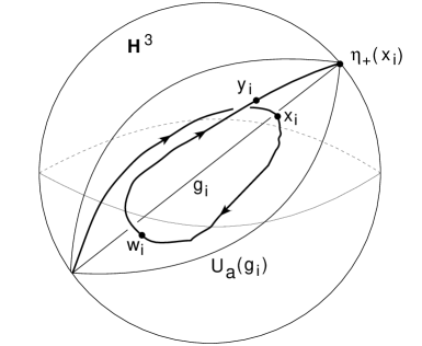
Since $d(w_{i},x_{i})\rightarrow+\infty$ these arguments show that in any case there are $x_{i},y_{i}\in\widetilde{Y}$, with $\rho_{i}(x_{i})=\rho_{i}(y_{i})$, $(x_{i},y_{i})\subset B(x_{i},g_{i})$ and diam$[x_{i},y_{i}]\rightarrow+\infty$, see figure 1. Up to covering translations and taking a subsequence we may assume that $x_{i}\rightarrow x\in\widetilde{Y}$. Since $g_{i}=g_{x_{i}}\rightarrow g_{x}$ and $\rho_{i}(x_{i})=\rho_{x_{i}}(x_{i})\rightarrow\rho_{x}(x)$, then

$${\overline{P(\rho_{x_{i}}(x_{i})+2,g_{i})}}\ \rightarrow\ {\overline{P(\rho_{x}(x)+2,g_{x})}}$$

in the topology of closed sets of $\mbox{${\bf H}^{3}$}\cup\mbox{$S^{2}_{\infty}$}$. Then

$$\eta_{+}(x)\in{\overline{F(\rho_{x_{i}}(x_{i})+1,g_{i})}}$$

for $i$ big enough. Hence there is $t_{0}>0$ so that for $i$ big enough $x\cdot[t_{0},+\infty)\subset F(\rho_{x_{i}}(x_{i}),g_{i})$. It therefore follows that for $i$ big enough there is $r_{i}$ with $r_{i}<t_{0}+1$ and $x_{i}\cdot r_{i}\in F(\rho_{x_{i}}(x_{i}),g_{i})$. This contradicts the facts $(x_{i},y_{i})\subset B(\rho_{x_{i}}(x_{i}),g_{i})$ with $y_{i}=x_{i}\cdot t_{i}$ and $t_{i}\rightarrow+\infty$. This finally finishes the proof of theorem 1.4. ∎

Remarks:

(1) The above proof works verbatim for $M^{n}$ closed hyperbolic.

(2) Without much more work, one can also prove this result under more general assumptions:

(i) $M$ is any manifold and $\pi_{1}(M)$ is word hyperbolic in the sense of Gromov [Gr]. In that case instead of $S^{2}_{\infty}$ one uses the appropriate boundary at infinity $\partial_{\infty}\mbox{$\widetilde{M}$}$ — notice that if $M$ is an oriented, irreducible 3-manifold then $\partial_{\infty}\mbox{$\widetilde{M}$}$ is still a $2$-dimensional sphere [Be-Me].

(ii) $Y$ is a compact space on which a flow $\Phi$ is defined, and instead of $Y$ being a subset of $M$ we have instead a continuous function $f\colon Y\to M$. By the pullback construction we have $f\colon\widetilde{Y}\to\widetilde{M}$ and a flow $\widetilde{\Phi}$ on $\widetilde{Y}$, and theorem 1.4 applies.

2. Hierarchies

Finite depth foliations are closely related to sutured manifold hierarchies [Ga1]. In [Ga3] an “internal” version of a sutured manifold hierarchy was defined, in terms of branched surfaces. We review this subject here, providing some proofs of known but unpublished information, and we add some geometric information. For detailed definitions concerning foliations and laminations on 3-manifolds see [Ga1] and [Ga-Oe].

A $2$-dimensional foliation of a 3-manifold $M$ is a decomposition of $M$ into $2$-dimensional manifolds called leaves which fit together in a local product structure. A foliation $\mathcal{F}$ is taut if it is transversely oriented, no leaf is a sphere, and each leaf of $\mathcal{F}$ intersects some closed curve in $M$ which is transverse to $\mathcal{F}$. The leaves of a taut foliation are $\pi_{1}$-injective [No].

A lamination of $M$ is a foliation of a closed subset of $M$, covered by charts of the form $D^{2}\times[0,1]$ so that each component of a leaf intersected with the chart has the form $D^{2}\times t$ for some $t\in[0,1]$. A lamination $\Lambda$ is essential if it has no sphere leaves, no Reeb components, and if $M_{\Lambda}$ is the metric completion of $M-\Lambda$, then $M_{\Lambda}$ is irreducible, boundary incompressible, and end incompressible; the latter condition means intuitively that $\partial M_{\Lambda}$ has no “infinite folds”. The leaves of an essential lamination $\Lambda$ are $\pi_{1}$-injective in $M$, and the components of $M-\Lambda$ are $\pi_{1}$-injective.

A taut foliation is obviously an essential lamination. It is an exercise in the results of [Ga-Oe] to show that every sublamination of an essential lamination is essential.

Given a foliation $\mathcal{F}$ in a closed manifold $M$ we say that a leaf $L$ of $\mathcal{F}$ is proper if $\overline{L}-L$ is a closed subset of $M$ and $\mathcal{F}$ is proper if all leaves are proper. In that case Zorn’s lemma implies that $\mathcal{F}$ has compact leaves, which are then the depth 0 leaves. The depth is an ordinal $\omega$ defined by induction: a leaf $L$ is at depth $\omega$ if $\overline{L}-L$ is contained in the union of leaves of depth $<\omega$, but not contained in the union of leaves $<\omega_{1}$ for any $\omega_{1}<\omega$. A proper foliation has finite depth $n$ if $n$ is the maximum of the depth of its leaves.

A branched surface in a closed 3-manifold $M$ is a smooth 2-complex $B\subset M$ such that for each $x\in B$, there exists a smoothly embedded open disc in $B$ containing $x$, and all such discs are tangent at $x$, therefore determining a well-defined tangent plane $T_{x}B$. The set of points where $B$ is not locally a surface is called the branch locus. A sector of $B$ is a complementary component of the branch locus. In this paper, all branched surfaces will be transversely oriented. A flow (or semiflow) is transverse to $B$ if, for each $x\in B$, the tangent vector to the flow points to the same side of $T_{x}B$ as the transverse orientation.

Given a branched surface $B\subset M$, a semiflow neighborhood $U(B)$ is a piecewise smooth regular neighborhood equipped with a semiflow $\varphi$ satisfying the following conditions. Each orbit of $\varphi$ is compact, transverse to $B$, and pierces $B$ in at least one point. There is a decomposition of $\partial U(B)$ into subsurfaces with disjoint interior

$$\partial U(B)=\partial_{v}U(B)\cup\partial_{h}^{-}U(B)\cup\partial_{h}^{+}U(B)$$

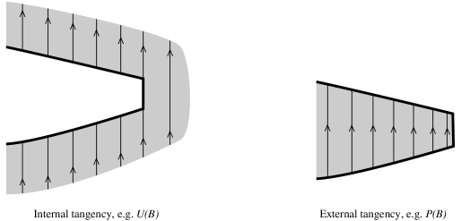
such that orbits of $\varphi$ point inward along $\partial_{h}^{-}U(B)$, outward along $\partial_{h}^{+}U(B)$, and are internally tangent along $\partial_{v}U(B)$ as shown in figure 2. Each component of $\partial_{v}U(B)$ is an annulus and the orbits of $\varphi$ define a fibration of the annulus over the circle with interval fiber. If one forgets the orientation and parameterization of $\varphi$, one obtains an $I$-bundle neighborhood of $B$ as in [Ga-Oe].

Figure 2. Boundary tangencies of semiflows

We shall regard the exterior of $U(B)$ as a sutured manifold, as follows.

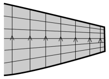
A sutured manifold is an oriented 3-manifold $P$ whose boundary is decomposed into surfaces with disjoint interior as $\partial P={\mathcal{R}}_{-}P\cup{\mathcal{R}}_{+}P\cup{\mathcal{A}}P$, where ${\mathcal{R}}_{-}P$ and ${\mathcal{R}}_{+}P$ are disjoint, ${\mathcal{A}}P$ is a collection of annuli called the sutures, ${\mathcal{R}}_{-}P\cap{\mathcal{A}}P=\partial({\mathcal{R}}_{-}P)\subset\partial({\mathcal{A}}P)$, ${\mathcal{R}}_{+}P\cap{\mathcal{A}}P=\partial({\mathcal{R}}_{+}P)\subset\partial({\mathcal{A}}P)$, and each component of ${\mathcal{A}}P$ has one boundary component in ${\mathcal{R}}_{-}P$ and the other in ${\mathcal{R}}_{+}P$. Let ${\mathcal{R}}_{\pm}P={\mathcal{R}}_{-}P\cup{\mathcal{R}}_{+}P$. A sutured manifold $P$ is a product if there is a homeomorphism $(P,{\mathcal{A}}P)\approx(S\times I,\partial S\times I)$ for some compact surface $S$. Given a semiflow on a sutured manifold $P$, we say that $P$ is an isolating block for the semiflow if orbits point outward along ${\mathcal{R}}_{+}P$, inward along ${\mathcal{R}}_{-}P$, and are externally tangent along $\gamma P$ as shown in figure 2. A foliation of a sutured manifold $P$ is required to be tangent to ${\mathcal{R}}_{\pm}P$ and transverse to ${\mathcal{A}}P$. Near ${\mathcal{A}}P$, a transverse foliation and semiflow appear in cross section as in figure 3.

Figure 3. A foliation and semiflow on a sutured manifold.

If $B\subset M$ is a branched surface then $P(B)=\operatorname{cl}(M-U(B))$ has the structure of a sutured manifold where $R_{+}P(B)=\partial_{h}^{-}U(B)$, $R_{-}P(B)=\partial_{h}^{+}U(B)$, and ${\mathcal{A}}P(B)=\partial_{v}U(B)$. Given a flow $\varphi$ on $M$ transverse to $B$, there exists a regular neighborhood $U(B)$ so that the restriction of $\varphi$ makes $U(B)$ into a semiflow neighborhood, and so that $P(B)$ is an isolating block for $\varphi$. We say that $U(B)$ is adapted to $\varphi$.

A hierarchy on $M$, in the sense of Gabai, is a sequence of branched surfaces $B_{0}\subset B_{1}\subset\cdots\subset B_{N}$ such that $B_{0}$ is a surface, $B_{n}-B_{n-1}$ is a union of sectors of $B_{n}$ for each $1\leq n\leq N$, and $P(B_{N})$ is a product. Let $S(B_{n})=B_{n}\cap P(B_{n-1})$; this is a transversely oriented surface properly embedded in $P(B_{n-1})$, and it is obtained from the sectors $B_{n}-B_{n-1}$ by removing an open collar of each boundary component. We may assume that each component $c$ of $\partial S(B_{n})$ satisfies the property that either $c$ is a core curve of some suture of $P(B_{n-1})$ or $c$ is transverse to the sutures, meaning that each component of $c\cap{\mathcal{A}}P(B_{n-1})$ is an arc connecting opposite boundaries of some component of ${\mathcal{A}}P(B_{n-1})$. This property is immediate if each component of the boundary of $B_{n}-B_{n-1}$ either is in general position with respect to the branch locus of $B_{n-1}$, or is contained in the branch locus. Otherwise, this property can be achieved by first choosing $U(B_{n-1})$ so that the annuli of $\partial_{v}U(B_{n-1})$ are extremely thin, and then doing a small isotopy of $S(B_{n})$. Note that $P(B_{n})$ is obtained by doing a sutured manifold decomposition of $P(B_{n-1})$ along $S(B_{n})$, in the sense of [Ga1].

Let $\mathcal{F}$ be a transversely oriented foliation in $M$, with a fixed transversal flow $\varphi$. Given a saturated open set $W$, let $\widehat{W}$ be its metric completion. The inclusion $\iota\colon W\hookrightarrow M$ extends to an immersion $\hat{\iota}\colon\widehat{W}\rightarrow M$ carrying each component of $\partial\widehat{W}$ diffeomorphically onto a leaf of $\mathcal{F}$, but $\hat{\iota}$ may identify some of these boundary components pairwise. In addition the structure of the foliation in $\widehat{W}$ is as follows [Di, Ca-Co]: $\widehat{W}=Q\cup(\Sigma\times I)$, where $Q$ is a compact (possibly empty) sutured manifold, each component of $\Sigma$ is a noncompact surface with compact connected boundary, $Q$ is glued to $\Sigma\times I$ by identifying ${\mathcal{A}}Q$ with $\partial\Sigma\times I$, and the restrictions of $\mathcal{F}$ and $\varphi$ to $Q$ and to $\Sigma\times I$ are well-behaved as follows. The restrictions to $Q$ give a sutured manifold foliation and semiflow; and the restriction of $\varphi$ to $\Sigma\times I$ is a product flow, that is, orbits have the form $x\times I$. Note that the restriction of $\mathcal{F}$ to $\Sigma\times I$ need not have leaves of the form $\Sigma\times t$. If a connected open saturated set $W$ has $Q=\emptyset$, then $\widehat{W}$ (or $W$) is called a foliated product. An important fact is that for any saturated open set $W$, at most finitely many components of $W$ are not foliated products [Di, Ca-Co].

The results above are also true for foliations of sutured manifolds. To see this, first double along the sutures and then double along the remaining boundary and apply the result to the final closed manifold.

Proposition 2.1.

(hierarchy exists) If $\mathcal{F}$ is a taut finite depth foliation on $M$ and $\varphi$ is a flow transverse to $\mathcal{F}$, then there exists a hierarchy $B_{0}\subset\cdots\subset B_{N}$ transverse to $\varphi$ with neighborhoods $U(B_{0})\subset\cdots\subset U(B_{N})$ adapted to $\varphi$, such that the sutured manifolds $P(B_{n})$ and the surfaces $S(B_{n})$ are $\pi_{1}$-injective in $M$, and each component of $B_{0}$ is isotopic to a compact leaf of $\mathcal{F}$.

The construction of finite depth foliations in theorem 5.1 of [Ga1] proceeds by first constructing a hierarchy and then using it to produce the foliation. The point of this proposition is that all finite depth foliations arise by this construction; and we obtain additional information about flows. Since we cannot find a published proof we provide one, though the ideas are well-known.

Proof.

Let $\mbox{$\mathcal{F}$}_{n}$ be the union of leaves of $\mathcal{F}$ of depth at most $n$. Since $\mathcal{F}$ is proper, $\mbox{$\mathcal{F}$}_{n}$ is closed, hence it is a sublamination of $\mathcal{F}$, therefore an essential lamination in $M$. Let $M_{n}=M-\mbox{$\mathcal{F}$}_{n}$, and $\widehat{M}_{n}$ its metric completion. Then at most finitely many components of $M_{n}$ are not foliated products. Now we may alter $\mathcal{F}$ without altering $\varphi$, collapsing foliated product components of $M_{n}$; do this inductively for each $n$. After the alterations, only finitely many leaves are isolated, where a leaf $L$ at depth $n$ is said to be isolated if $L$ is isolated in $\mbox{$\mathcal{F}$}_{n}$. In addition if $L$ at depth $n$ is not isolated, then the component of $\mbox{$\mathcal{F}$}_{n}-\mbox{$\mathcal{F}$}_{n-1}$ containing $L$ fibers over the circle with fiber $L$. Next fatten up each of the finitely many isolated leaves into a fibration over a closed interval, again altering $\mathcal{F}$ without altering $\varphi$. Each connected component of $\mbox{$\mathcal{F}$}_{n}-\mbox{$\mathcal{F}$}_{n-1}$ is now either a fibration over a closed interval, or a fibration over the circle; the latter are called “circular” components of $\mbox{$\mathcal{F}$}_{n}-\mbox{$\mathcal{F}$}_{n-1}$. Under these condition $\widehat{M}_{n}$ is a 1-1 immersed submanifold of $M$ whose boundary components are leaves of $\mbox{$\mathcal{F}$}_{n}$.

Now we construct by induction a hierarchy $B_{0}\subset\cdots\subset B_{N}$ and neighborhoods $U(B_{0})\subset\cdots\subset U(B_{N})$ adapted to $\varphi$ so that if $0\leq n\leq N$ then:

1. $U(B_{n})$ contains every noncircular component of $\mbox{$\mathcal{F}$}_{n}-\mbox{$\mathcal{F}$}_{n-1}$, as well as an interval’s worth of leaves in every circular component.

2. $\mathcal{F}$ restricts to a foliation of the sutured manifold $P(B_{n})=\overline{\bigl{(}M-U(B_{n})\bigr{)}}.$ It may be a product foliation in some components of $P(B_{n})$.

3. The embedding $P(B_{n})\hookrightarrow P(B_{n-1})$ is $\pi_{1}$-injective.

4. $S(B_{n})=B_{n}\cap P(B_{n-1})$ is $\pi_{1}$-injective in $P(B_{n-1})$.

If $\mathcal{F}$ is not a fibration over $S^{1}$, let $U(B_{0})$ to be the union of the compact leaves, otherwise let $U(B_{0})$ be a closed interval of leaves. Properties (1–2) are evident. We interpret (3) and (4) by setting $P(B_{-1})=M$, and these properties follow because the compact leaves of $\mathcal{F}$ are incompressible surfaces in $M$.

To continue the induction, given a component $Z$ of $P(B_{n})$ on which the restriction of $\mathcal{F}$ and $\varphi$ does not already give a product structure, we describe the intersections with $Z$ of $P(B_{n+1})$, $U(B_{n+1})$, and $B_{n+1}$ itself. Let $V(\partial_{\pm}Z)$ be a neighborhood so that the restriction of $\phi$ has compact orbits, defining a product structure with projection map $q\colon V(\partial_{\pm}Z)\to\partial_{\pm}Z$.

Let $\mbox{$\mathcal{F}$}^{\prime}$ be the restriction of $\mbox{$\mathcal{F}$}_{n+1}$ to $Z$. This lamination has depth $\leq 1$. Its compact leaves consist of $\partial_{\pm}Z$ plus foliated products $F\times I$ with $\partial F\times I\subset{\mathcal{A}}Z$; all but finitely many of these foliated products have leaves parallel to a component of $\partial_{\pm}Z$. The noncompact leaves of $\mbox{$\mathcal{F}$}^{\prime}$ fall into a finite collection of circular components and foliated products, and each end $E$ of a noncompact leaf $L$ spirals into some component $F$ of $\partial_{\pm}Z$ in the following manner: there is a nonseparating, properly embedded, connected 1-manifold $c\subset F$ called a juncture for $E$, there is a ${\bf Z}$-covering space $\tilde{F}\to F$ to which $c$ lifts homeomorphically, there is a subset $L_{E}\subset L$ representing $E$ and contained in $V(F)$ (the component of $V(\partial_{\pm}Z)$ containing $F$), and there is an embedding $L_{E}\to\tilde{F}$, such that the maps $L_{E}\to\tilde{F}\to F$ and $L_{E}\hookrightarrow V(F)\to F$ are the same, and the image of $\partial L_{E}$ is the curve $c$. If $E,E^{\prime}$ are ends of noncompact leaves spiralling into the same component $F$ of $\partial_{\pm}Z$, and if $E,E^{\prime}$ are not in the same end of a circular component of $\mbox{$\mathcal{F}$}^{\prime}$, we may assume that the junctures for $E,E^{\prime}$ are disjoint but isotopic curves in $F$.

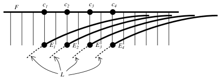
Let $\mbox{$\mathcal{F}$}^{\prime\prime}$ be the union of the finitely many foliated products in $\mbox{$\mathcal{F}$}^{\prime}$ which are not contained in $V(\partial_{\pm}Z)$, plus a closed interval of leaves in each circular component of $\mbox{$\mathcal{F}$}^{\prime}$, plus $\partial_{\pm}Z$. Since $Z-\mbox{$\mathcal{F}$}^{\prime\prime}$ is an open subset of $Z$ saturated by $\mbox{$\mathcal{F}$}\bigm{|}Z$, letting ${\overline{Z-\mbox{$\mathcal{F}$}^{\prime\prime}}}$ be the metric completion of $Z-\mbox{$\mathcal{F}$}^{\prime\prime}$, there is a decomposition ${\overline{Z-\mbox{$\mathcal{F}$}^{\prime\prime}}}=Q\cup(\Sigma\times I)$ where $Q$ is a compact sutured manifold and $\Sigma\times I$ is a foliated product so that each noncompact component of $\Sigma$ has compact, connected boundary. We can choose $Q$ big enough so that $\Sigma\times I$ is contained in $V(\partial_{\pm}Z)$, and so that the boundary of each component of $\Sigma$ projects to some juncture, thus we can associate a juncture to each component of $\Sigma$. Moreover, if $\Sigma_{1},\ldots,\Sigma_{n}$ are components of $\Sigma$ with isotopic junctures $c_{1},\ldots,c_{n}$ lying in a component $F$ of $\partial_{\pm}Z$, then we can choose $Q$ so that the picture in figure 4 holds: the curves $c_{1},\ldots,c_{n}$ are ordered so that $c_{i}\cup c_{i+1}$ bounds an annulus disjoint from the other curves; and the “first hitting” map $\Sigma_{i+1}\to\Sigma_{i}$ is continuous for $i=1,\ldots,n-1$, where this map is defined by starting from a point in $\Sigma_{i+1}$, going along an orbit of $\phi$ towards $F$, and stopping at the first point of $\Sigma_{i}$.

Figure 4. Isotopic junctures

Now define $P(B_{n+1})\cap Z=Q$. Notice that $\mbox{$\mathcal{F}$}^{\prime\prime}$ is an essential lamination of $Z$, hence $Z-\mbox{$\mathcal{F}$}^{\prime\prime}$ is $\pi_{1}$-injective in $Z$. Since each noncompact component of $\Sigma$ has compact, connected boundary, it follows that $Q$ is $\pi_{1}$-injective in $Z-\mbox{$\mathcal{F}$}^{\prime\prime}$, and property (3) for $P(B_{n+1})$ follows. Property (2) is easily checked, as is property (1) for $U(B_{n+1})={\overline{(M-P(B_{n+1}))}}$.

To define the sectors of $B_{n+1}$ intersecting $Z$, note that the foliation and flow define a product structure $\mbox{$\mathcal{F}$}^{\prime\prime}-\partial_{\pm}Z=G\times[0,1]$ for some surface $G$, not necessarily connected. Each end of $G\times 0$ or $G\times 1$ is eventually contained in $\Sigma\times I$. Let $L$ be the set of $x\in G$ such that $x\times[0,1]$ is disjoint from $\Sigma\times I$. Then $L$ is a subsurface of $G$, and we may regard $L$ as being embedded in $\mbox{$\mathcal{F}$}^{\prime\prime}$ transverse to the flow. Homotop $\partial L$ to a map into $B_{n}$ as described below, and extend the homotopy over $L$. The image of $L$ after the homotopy is the union of sectors of $B{n+1}-B_{n}$ intersecting $Z$. To describe the homotopy of $\partial L$, each component $\beta$ of $\partial L-{\mathcal{A}}Z$ lies in $V(\partial_{\pm}Z)$, and $\beta$ projects via $\phi$ to a juncture; homotop $\partial L$ along orbits of $\phi$ until $\beta$ lies on that juncture. Extend the homotopy of $\partial L-{\mathcal{A}}Z$ over all of $\partial L$, so that each arc component of $\partial L\cap{\mathcal{A}}Z$ maps to an arc in $B_{n}$ crossing the branch locus in a single transverse intersection point, and each circle component of $\partial L\cap{\mathcal{A}}Z$ maps to a circle in the branch locus of $B_{n}$. Because of the properties of junctures given in figure 4, this homotopy may be carried out so that $L-\partial L$ is embedded in $M-B_{n}$, and hence the image of $L$ after the homotopy consists of sectors of $B_{n+1}-B_{n}$ whose boundary lies in $B_{n}$, as required for a hierarchy.

Property (4) for $S(B_{n+1})$ follows because each component of $S(B_{n+1})$ corresponds to a component of $L$ as above, but components of $L$ are $\pi_{1}$-injective in in $P(B_{n})$.

The only nonobvious points remaining in the proof of the lemma are the statements on $\pi_{1}$-injectivity. Using (3) it follows by induction that $P(B_{n})$ is $\pi_{1}$-injective in $M$. Using (4), and the fact that $P(B_{n-1})$ is $\pi_{1}$-injective in $M$, it follows that $S(B_{n})$ is $\pi_{1}$-injective in $M$. ∎

We also need some geometric information about hierarchies. Consider a closed, oriented 3-manifold $M$ and a nonseparating incompressible surface $F$. We say $F$ is a fiber if $F$ is a leaf of a fibration of $M$ over $S^{1}$. If $M$ is hyperbolic we say that $F$ is quasi-fuchsian if the representation $\pi_{1}F\to\pi_{1}M\to\operatorname{Isom}({\bf H}^{3})$ is quasi-fuchsian. A deep fact due to Marden [Ma], Thurston [Th1] and Bonahon [Bo], is that when $M$ is hyperbolic then $F$ is either a fiber or quasi-fuchsian (if $F$ is separating there is another option, namely that $F$ is a “virtual fiber”).

Recall from [Gr, Gh-Ha] that a locally compact path metric space $X$ is negatively curved in the large if it satifies the “thin triangles” condition: there exists $\delta>0$ such that for every geodesic triangle with sides $A_{1},A_{2},A_{3}$ we have $A_{1}\subset U_{\delta}(A_{2}\cup A_{3})$. In this case there is a canonically defined ideal boundary at infinity denoted $\partial_{\infty}X$, and there is a canonical compactification $X\cup\partial_{\infty}X$. If $X$ is negatively curved in the large, so is any space quasi-isometric to $X$. If $X,Y$ are negatively curved in the large and $f\colon X\to Y$ is a quasi-isometry then $f$ extends canonically to a continuous map $\hat{f}\colon X\cup\partial_{\infty}X\rightarrow Y\cup\partial_{\infty}Y$ that restricts to an embedding $\partial_{\infty}X\hookrightarrow\partial_{\infty}Y$. For example, hyperbolic space ${\bf H}^{n}$ is negatively curved in the large, and its ideal boundary in the sense of Gromov is the same as the sphere at infinity $S^{n-1}_{\infty}$. Also, any closed convex subset $X\subset{\bf H}^{n}$ is negatively curved in the large, and $\partial_{\infty}X$ coincides with the set of limit points of $X$ in $S^{n-1}_{\infty}$.

Given a group $G$ with a finite generating set $A$, the Cayley graph $C$ is the graph with a vertex for each $g\in G$, and an edge from $g$ to $ga$ for each $a\in A$. By taking each edge to be a path of length 1 we make the Cayley graph a path metric space. For any two finite generating sets, the Cayley graphs are quasi-isometric. The group $G$ is word hyperbolic if some (and hence any) Cayley graph of $G$ is negatively curved in the large. Then we let $\partial_{\infty}G=\partial_{\infty}C$. Consider a compact Riemannian manifold $M$ with $G=\pi_{1}(M,x)$, choose a lift $x_{0}$ of $x$ in the universal cover $\widetilde{M}$ and choose loops in $M$ representing a finite generating set for $\pi_{1}(M)$. Lifting to $\widetilde{M}$ we have a map of the Cayley graph of $G$ to $\widetilde{M}$, which gives a quasi-isometry between $G$ and $\widetilde{M}$ [Mi]. Therefore $G=\pi_{1}M$ is word hyperbolic if and only if $\widetilde{M}$ is negatively curved in the large, in which case there is a canonical identification $\partial_{\infty}G\approx\partial_{\infty}\widetilde{M}$.

Proposition 2.2.

Let $M$ be a closed, orientable hyperbolic 3-manifold, $B_{0}\subset\cdots\subset B_{N}$ a hierarchy in $M$ such that $P(B_{n})$ and $S(B_{n})=B_{n}\cap P(B_{n-1})$ are $\pi_{1}$-injective for all $n$. Suppose that some component $F$ of $B_{0}$ is a quasi-fuchsian surface in $M$. Then:

(1) Each group $\pi_{1}(P(B_{n}))$, $\pi_{1}(S(B_{n}))$ is word hyperbolic.

(2) Each embedding $\widetilde{S}(B_{n})\hookrightarrow\widetilde{P}(B_{n-1})$ is a quasi-isometry which takes $\partial\widetilde{S}(B_{n})$ into $\partial\widetilde{P}(B_{n})$. Therefore it extends to an embedding $\widetilde{S}(B_{n})\cup\partial_{\infty}\widetilde{S}(B_{n})\hookrightarrow\widetilde{P}(B_{n-1})\cup\partial_{\infty}\widetilde{P}(B_{n-1})$.

(3) Each inclusion $\widetilde{P}(B_{n})\hookrightarrow\widetilde{P}(B_{n-1})$ is a quasi-isometry in the path metrics induced from $\widetilde{M}$. Therefore it extends to an embedding $\widetilde{P}(B_{n})\cup\partial_{\infty}\widetilde{P}(B_{n})\hookrightarrow\widetilde{P}(B_{n-1})\cup\partial_{\infty}\widetilde{P}(B_{n-1})$.

Remark: The group $\pi_{1}(S(B_{n}))$ may be cyclic, when $S(B_{n})$ is an annulus; or trivial, when $S(B_{n})$ is a disc.

Proof.

Let $\rho\colon\pi_{1}(M)\rightarrow PSL_{2}({\bf C})$ be the holonomy representation of the hyperbolic structure. Consider the subgroup $G=\rho(\pi_{1}(M-F))$ with limit set $\Lambda G\subset S^{2}_{\infty}$, let ${\mathcal{H}}(\Lambda G)\subset{\bf H}^{3}\cup S^{2}_{\infty}$ be its convex hull, let ${\mathcal{H}}_{\epsilon}(\Lambda G)\subset{\bf H}^{3}\cup S^{2}_{\infty}$ be the union of ${\mathcal{H}}(\Lambda G)$ with its $\epsilon$-neighborhood in ${\bf H}^{3}$, and let $X_{G}={\mathcal{H}}_{\epsilon}(\Lambda G)\cap{\bf H}^{3}$. Since $F$ is quasi-Fuchsian, the group $G$ is convex cocompact, that is $G$ acts cocompactly on $X_{G}$; equivalently, $G$ is geometrically finite [Ma, Th1]. It follows that any finitely generated subgroup $H<G$ is convex cocompact [Th1, Cn]. Since $X_{H}$ is negatively curved in the large, and the action of $H$ on $X_{H}$ is properly discontinuous and cocompact, it follows that $H$ is word hyperbolic, proving (1).

Suppose $P\subset M-F$ is a compact, $\pi_{1}$-injective submanifold and $H=\pi_{1}(P)$. We show that the natural inclusion $j\colon\widetilde{P}\to{\bf H}^{3}$ is a quasi-isometric embedding, where $\widetilde{P}$ has the path metric induced from $\widetilde{M}$.

The natural inclusion $\iota\colon X_{H}\hookrightarrow{\bf H}^{3}$ is a quasi-isometric embedding. Let $\Gamma_{H}$ be the Cayley graph of $H$, and consider the two quasi-isometries $\alpha\colon\Gamma_{H}\to X_{H}$, $\beta\colon\Gamma_{H}\to\widetilde{P}$ given by [Mi]. The maps $\iota\circ\alpha,j\circ\beta\colon\Gamma_{H}\to{\bf H}^{3}$ differ by a bounded amount, therefore $j\circ\beta$ is a quasi-isometric embedding. There is a quasi-isometry $\bar{\beta}\colon\widetilde{P}\to\Gamma_{H}$ which is an inverse of $\beta$ in the quasi-isometric category, so in particular $\beta\circ\bar{\beta}\colon\widetilde{P}\to\widetilde{P}$ differs from the identity by a bounded amount. Thus we have a quasi-isometric embedding $j\circ\beta\circ\bar{\beta}\colon\widetilde{P}\to{\bf H}^{3}$ which differs from $j$ by a bounded amount, so $j$ is a quasi-isometric embedding. Hence each $\widetilde{P}(B_{n})\hookrightarrow\mbox{${\bf H}^{3}$}$ extends to a continuous embedding $\widetilde{P}(B_{n})\cup\partial_{\infty}\widetilde{P}(B_{n})\hookrightarrow\mbox{${\bf H}^{3}$}\cup\mbox{$S^{2}_{\infty}$}$.

To prove (3), the quasi-isometric embedding $\widetilde{P}(B_{n})\hookrightarrow{\bf H}^{3}$ factors through the natural embedding $\widetilde{P}(B_{n})\hookrightarrow\widetilde{P}(B_{n-1})$, so $\widetilde{P}(B_{n})\hookrightarrow\widetilde{P}(B_{n-1})$ is a quasi-isometric embedding. The proof of (2) is similar. ∎

Remark: Although not logically necessary for our results, it is helpful to keep in mind the following additional facts:

(4) Each compactified universal cover $\widetilde{P}(B_{n})\cup\partial_{\infty}\widetilde{P}(B_{n})$ is a 3-ball.

(5) Each $\widetilde{S}(B_{n})\cup\partial_{\infty}\widetilde{S}(B_{n})$ is a 2-disc properly embedded in the above 3-ball.

To prove (4), let $P=P(B_{n})$, let $H=\pi_{1}(P)$, and consider the action of $H$ on ${\bf H}^{3}$. In the manifold ${\bf H}^{3}/H$, both of the compact manifolds $X_{H}/H$ and $P$ embed as deformation retracts. By [Mc-MS] it follows that there is a homeomorphism $X_{H}/H\approx P$ in the correct homotopy class. This homeomorphism lifts to an $H$-equivariant quasi-isometric homeomorphism $X_{H}\approx\widetilde{P}$, which extends to a homeomorphism ${\mathcal{H}}_{\epsilon}(\Lambda H)\approx\widetilde{P}\cup\partial_{\infty}\widetilde{P}$, and ${\mathcal{H}}_{\epsilon}(\Lambda H)$ is obviously a 3-ball.

The proof of (5) when $S(B_{n})$ is a disc or annulus is easy. Otherwise there is a hyperbolic metric with geodesic boundary on $S(B_{n})$, and $\widetilde{S}(B_{n})\cup\partial_{\infty}S(B_{n})$ is therefore a 2-disc, which by (2) is properly embedded in the 3-ball $\widetilde{P}\cup\partial_{\infty}\widetilde{P}$.

3. Inductive proof of theorem A

To set up the induction, apply proposition 2.1 to obtain a hierarchy $B_{0}\subset\cdots\subset B_{N}$. We use the following notation. If $0\leq n\leq N$ let $P_{n}=P(B_{N-n})$, and let $P_{N+1}=M$, so $P_{0}\subset P_{1}\subset\cdots\subset P_{N}\subset P_{N+1}$; the indexing is reversed to facilitate the induction proof. If $1\leq n\leq N+1$ let $S_{n}=S(B_{N-n+1})=B_{N-n+1}\cap P_{n}$, so $S_{n}$ is properly embedded in $P_{n}$, and $P_{n-1}$ is obtained from $P_{n}$ by removing a regular neighborhood of $S_{n}$. Since some (and hence all) compact leaves of $\mathcal{F}$ are quasi-fuchsian, the same is true for components of $B_{0}$, hence proposition 2.2 applies.

Given a flow line $x\cdot{\bf R}$ of $\Phi$, define the codepth to be the minimal integer $n$ such that $x\cdot{\bf R}\subset P_{n}$, and define $\Omega_{n}$ to be the union of all flow lines of codepth at most $n$. Note that $\Omega_{n}$ is the set of all flow lines contained in $P_{n}$, and $\Omega_{n}$ is closed. As special cases, $\Omega_{0}=\emptyset$ since $P_{0}$ is a product, and $\Omega_{N+1}=M$.

The program for the proof of theorem A is to assume that orbits in $\Omega_{n-1}$ are uniformly quasigeodesic and then show that orbits in $\Omega_{n}$ are also uniformly quasigeodesic (with a bigger quasigeodesic constant). Since $\Omega_{0}=\emptyset$ and $\Omega_{N+1}=M$, induction will show that all orbits are uniformly quasigeodesic. This will complete the proof of theorem A.

For notational convenience, throughout this section we write $P=P_{n}$, $\Omega=\Omega_{n}$, $S=S_{n}$, $P^{\prime}=P_{n-1}$, and $\Omega^{\prime}=\Omega_{n-1}$. Let $\pi\colon\widetilde{P}\to P$ be the universal covering, and let $\widetilde{\Omega}=\pi^{-1}(\Omega)$.

Fix a connected lift $\widetilde{P}^{\prime}\hookrightarrow\widetilde{P}$, and let $\widetilde{\Omega}^{\prime}=\pi^{-1}(\Omega^{\prime})\cap\widetilde{P}^{\prime}$. The induction hypothesis says that orbits in $\widetilde{\Omega}^{\prime}$ are uniform quasigeodesics in $\widetilde{P}^{\prime}$. Since $\widetilde{P}^{\prime}\hookrightarrow\widetilde{P}$ is a quasi-isometry, then orbits in $\widetilde{\Omega}^{\prime}$ are uniformly quasigeodesic in $\widetilde{P}$; using the action of $\pi_{1}P$ by isometries on $\widetilde{P}$, the same is true for orbits in $\pi^{-1}(\Omega^{\prime})$. Recall that the hypothesis in theorem $A$ is that $\widetilde{\Phi}$ has Hausdorff orbit space. This will be used in verifying conditions (b) and (c) of theorem 1.4.

We will need the following well known simple result [Co]:

Lemma 3.1.

Let $W$ be a compact metric space with a nonsingular semiflow $\varphi$ parameterized by arc length. Let $\Omega$ be the set of points $x$ for which $\varphi_{t}(x)$ is defined for all $t\in\mbox{${\bf R}$}$. Then given any $\delta>0$, there is $a>0$ so that any orbit $\gamma$ of $\varphi$ is in the $\delta$-neighborhood of $\Omega$ except perhaps for an initial segment of length $<a$ and another final segment of length $<a$.

We will also use the following localization property of quasigeodesics.

Proposition 3.2.

[Gr, Gh-Ha] Let $M$ be a compact manifold with negatively curved $\pi_{1}(M)$. Then for any $K>0$ there is $L(K)>0$ (usually $L(K)>>K$) satisfying: if $\gamma$ is an embedded curve so that any subarc of length $\leq L(K)$ is a $K$ quasigeodesic then $\gamma$ is a $2K$-quasigeodesic.

The following essential fact which is a direct consequence of proposition 2.2 will be used explicitly or implicitly throughout this section: if $\gamma$ is a curve contained in $\widetilde{P}^{\prime}$, then $\gamma$ is a quasigeodesic in $\widetilde{P}^{\prime}$ if and only if $\gamma$ is a quasigeodesic in $\widetilde{P}$ and also if and only if $\gamma$ is a quasigeodesic in ${\bf H}^{3}$. The quasigeodesic constants may differ. We caution the reader that some arguments are done in ${\bf H}^{3}$ while others are done in $\widetilde{P}$. The context makes it clear.

For flow segments disjoint from $S$, the following lemma establishes the quasigeodesic property directly.

Lemma 3.3.

There is $K>0$ so that all flow segments, half orbits or full orbits of $\widetilde{\Phi}$ contained in $\widetilde{P}^{\prime}$ are $K$-quasigeodesics of $\widetilde{P}$; translating by the action of $\pi_{1}(P)$, the same is true in any lift of $P^{\prime}$.

Proof.

The full orbits staying in $\widetilde{P}^{\prime}$ are precisely the orbits in $\widetilde{\Omega}^{\prime}$, which are $k$-quasigeodesic for some uniform $k$. Fix $\delta_{0}>0$, with $2k\delta_{0}<1$. Let $L=L(k+1)$ be given by proposition 3.2. Choose $\delta_{1}>0$ so that if $x,y\in\widetilde{P}$ and $d(x,y)<\delta_{1}$ then $d(x\cdot t,y\cdot t)<\delta_{0}$ for any $|t|<L$. Choose $a>0$ so that any orbit in $P^{\prime}$ is in the $\delta_{1}$-neighborhood of $\Omega^{\prime}$, except perhaps for initial and final segments of length $<a$.

Let now $x,y\in\widetilde{P}^{\prime}$ with $y=x\cdot t$. Choose a subsegment $\gamma=[z,w]\subset[x,y]$, with $z=x\cdot t_{1}$, $w=y\cdot t_{2}$, $0\leq t_{1}<a$ and $-a<t_{2}\leq 0$, so that $\gamma\subset U_{\delta_{1}}(\widetilde{\Omega}^{\prime})$. Let $\alpha=[z_{0},w_{0}]$ be a subarc of $\gamma$ with $0<t_{3}=\operatorname{\tau}(z_{0},w_{0})\leq L$. By the choice of $\delta_{1}$ it follows that there is $z_{1}\in\widetilde{\Omega}^{\prime}$, with $d(z_{0}\cdot t,z_{1}\cdot t)<\delta_{0}$, for any $|t|<L$. Since $z_{1}\cdot{\bf R}$ is a $k$-quasigeodesic then

$$\operatorname{\tau}(z_{0},w_{0})=t_{3}=\operatorname{\tau}(z_{1},z_{1}\cdot t_{3})\leq k\,d(z_{1},z_{1}\cdot t_{3})+k$$

$$\leq kd(z_{0},w_{0})+2k\delta_{0}+k<kd(z_{0},w_{0})+(k+1).$$

Clearly this also works for any subsegment of $\alpha$, hence $\alpha$ is a $(k+1)$-quasigeodesic. By the previous proposition, one concludes that $\gamma$ is a $(2k+2)$-quasigeodesic. This implies that

$$\operatorname{\tau}(x,y) <2a+\operatorname{\tau}(z,w)\leq(2k+2)d(z,w)+(2k+2+2a)$$

$$\leq(2k+2)\bigl{(}d(x,y)+2a\bigr{)}+(2k+2+2a)$$

$$=(2k+2)d(x,y)+\bigl{(}2k+2+2a+(2k+2)2a\bigr{)}$$

Hence any piece of orbit of $\widetilde{\Phi}$ contained in $\widetilde{P}^{\prime}$ is a $(4ka+2k+6a+2)$-quasigeodesic of $\widetilde{P}^{\prime}$. Since $\widetilde{P}^{\prime}$ is quasi-isometrically embedded in $\widetilde{P}^{\prime}$, there is $K>0$ so that any piece of orbit of $\widetilde{\Phi}$ contained in $\widetilde{P}$ is a $K$-quasigeodesic of $\widetilde{P}$. ∎

Now we prepare the ground for applying theorem 1.4 to show that full orbits in $\widetilde{\Omega}$ are uniformly quasigeodesic. We must study how orbits in $\widetilde{\Omega}-\widetilde{\Omega}^{\prime}$ cross lifts of $S$ in $\widetilde{P}$, so we embark on a study of these lifts.

Let ${\mathcal{E}}$ be the collection of lifts of $S$ to $\widetilde{P}$. Any element $E\in{\mathcal{E}}$ is transversely oriented and separates $\widetilde{P}$. The front of $E$ is the component $\operatorname{Fr}(E)$ of $\widetilde{P}-E$ on the positive side of $E$, and the closure of $\operatorname{Fr}(E)$ in $\widetilde{P}\cup\partial_{\infty}\widetilde{P}$, is denoted $\sigma^{f}(E)$. The back $\operatorname{Bc}(E)$ and its closure $\sigma^{b}(E)$ are similarly defined. Define a strict partial order on $\mathcal{E}$ where $E<E^{\prime}$ if $\operatorname{Bc}(E)\cap\operatorname{Fr}(E^{\prime})=\emptyset$ and $E\not=E^{\prime}$, hence in particular $E^{\prime}\subset\operatorname{Fr}(E)$.

Notice that since $S$ is compact, a bounded subset of $\widetilde{P}$ intersects only finitely many $E\in{\mathcal{E}}$. The following lemmas strengthen this fact, by showing that sequences in $\mathcal{E}$ are limited in how they may accumulate in the ball $\widetilde{P}\cup\partial_{\infty}\widetilde{P}$; these lemmas will be useful in analyzing flow lines that cross $S$ many times. If $\rho:\pi_{1}(M)\rightarrow PSL_{2}({\bf C})$ is the holonomy representation, then $\rho(\pi_{1}(P))$ is a Kleinian group which is convex cocompact.

Lemma 3.4.

There is $J_{0}>0$ such that if $E_{1},\ldots,E_{J_{0}}$ are distinct elements of $\mathcal{E}$, then $\partial_{\infty}(E_{1})\cap\cdots\cap\partial_{\infty}(E_{J_{0}})=\emptyset$. If moreover $E_{1}<\cdots<E_{J_{0}}$ then $\sigma^{b}E_{1}\cap\sigma^{f}E_{J_{0}}=\emptyset$.

Proof.

First we need the fact that if $H_{1},\ldots,H_{n}$ are geometrically finite Kleinian groups that generate a discrete group, then $\Lambda H_{1}\cap\cdots\cap\Lambda H_{n}=\Lambda(H_{1}\cap\cdots\cap H_{n})$. When $n=2$ this is proved in [Su], and the statement for finitely many subgroups follows by induction.

To prove the first statement, suppose that $\partial_{\infty}(E_{1})\cap\cdots\cap\partial_{\infty}(E_{J})\neq\emptyset$. Let $H_{i}\subset\pi_{1}P$ be the stabilizer subgroup of $E_{i}$, so $\Lambda(H_{i})=\partial_{\infty}(E_{i})$, and by the above argument using Susskind’s theorem it follows that $H_{1}\cap\cdots\cap H_{J}\neq\emptyset$. Let $f$ be in the intersection, and let $\operatorname{Axis}_{f}$ be an axis for $f$ in ${\bf H}^{3}$. By conjugation, we may assume that $\operatorname{Axis}_{f}$ intersects a fixed fundamental domain $D$ for $\pi_{1}M$.

Since $E$ is quasi-isometrically embedded in ${\bf H}^{3}$, it is $R$-quasiconvex, that is, for any $x,y\in E\cup\partial_{\infty}E$, the geodesic in $E$ connecting them is at most $R$ distant from the hyperbolic geodesic connecting them [Gr, Gh-Ha]. The $R$ is independent of the lift $E$ of $S$. Thus each $E_{i}$ intersects $U_{R}(D)$, the open $R$-neighborhood of $D$. This shows that $J\leq J_{0}$ where $J_{0}$ is an upper bound for the number of distinct $E\in{\mathcal{E}}$ intersecting the bounded set $U_{R}(D)$.

To prove the second statement, suppose that $\sigma^{b}E_{1}\cap\sigma^{f}E_{J_{0}}\neq\emptyset$. It follows that $\partial_{\infty}E_{1}\cap\partial_{\infty}E_{J_{0}}\neq\emptyset$; let $\xi$ be a point in this intersection. If for some $1\leq i\leq n$, $\xi\not\in\partial_{\infty}E_{i}$, let $V$ be a neighborhood of $\xi$ in $\widetilde{P}\cap\partial_{\infty}\widetilde{P}$ with $E_{i}\cap(V\cap\widetilde{P})=\emptyset$. However since $\xi\in\partial_{\infty}E_{0}\cap\partial_{\infty}E_{J_{0}}$, there are $x\in E_{0}\cap V$ and $y\in E_{J_{0}}\cap V$. Hence $x$ can be connected to $y$ in $V\cap\widetilde{P}$, contradicting the fact that $E_{i}$ separates $E_{0}$ from $E_{J_{0}}$. But then we have proved $\partial_{\infty}E_{1}\cap\cdots\cap\partial_{\infty}E_{J_{0}}\neq\emptyset$, contradicting the first statement of the lemma. ∎

The $J_{0}$ given by the previous lemma is fixed from now on. The next lemma gives an even stronger accumulation property.

Lemma 3.5.

Given an infinite sequence $E_{1},E_{2},\ldots\in{\mathcal{E}}$ such that $E_{i}\neq E_{j}$ if $i\neq j$, suppose there exists $E_{0}\in{\mathcal{E}}$ such that $E_{0}<E_{i}$ for all $i\geq 1$. Then there is a subsequence $E_{i_{n}}$ such that $\sigma^{f}(E_{i_{n}})$ converges to a single point $\xi\in\partial_{\infty}\widetilde{P}$, in the Hausdorff topology on closed subsets of $\widetilde{P}\cup\partial_{\infty}\widetilde{P}$.

Proof.

Choose covering translations $f_{i}\in\pi_{1}P$ such that $f_{i}(E_{0})=E_{i}$. Then $f_{i}\neq f_{j}$ when $i\neq j$, so by the convergence group property for Kleinian groups applied to $\rho(\pi_{1}(M))$ (see pg. 22 of Maskit’s book [Ma]), we may pass to a subsequence so that there is a pair of points $\xi_{-},\xi_{+}\in\partial_{\infty}P$ called a source and sink for the sequence of functions $f_{i}$, meaning that $f_{i}\bigm{|}\bigl{(}\widetilde{P}\cup\partial_{\infty}\widetilde{P}\bigr{)}-\xi_{-}$ converges uniformly on compact sets to the constant map with value $\xi_{+}$, and $f_{i}^{-1}\bigm{|}\bigl{(}\widetilde{P}\cup\partial_{\infty}\widetilde{P}\bigr{)}-\xi_{+}$ converges similarly to $\xi_{-}$. Since $f_{i}^{-1}(\sigma^{b}(E_{i}))=\sigma^{b}(E_{0})$ for all $i$, it follows that $f_{i}^{-1}(\sigma^{b}(E_{0}))\subset\sigma^{b}(E_{0})$, and hence $\xi_{-}\in\sigma^{b}(E_{0})$.

If $\xi_{-}\in\sigma^{b}E_{0}-\partial_{\infty}E_{0}$ then we are done, because then $\xi_{-}\notin\sigma^{f}(E_{0})$, so the sequence of maps $f_{i}\bigm{|}\sigma^{f}(E_{0})$ converges uniformly to the constant map with value $\xi_{+}$, and hence the images $\sigma^{f}(E_{i})$ of these maps converge in the Hausdorff topology to $\xi_{+}$.

Suppose on the other hand that $\xi_{-}\in\partial_{\infty}E_{0}$. By the previous lemma, for all but finitely many $E_{i}$ we have $\xi_{-}\notin\partial_{\infty}E_{i}$; in particular this is true for some $i=i_{0}$. We also have $\xi_{-}\notin\sigma^{f}(E_{i_{0}})$, because $\xi_{-}\in\sigma^{b}(E_{0})$. Note that $\xi_{-},\xi_{+}$ is a source, sink pair for the sequence $f_{i}\circ f_{i_{0}}^{-1}$, so the maps $f_{i}\circ f_{i_{0}}^{-1}\bigm{|}\sigma^{f}(E_{i_{0}})$ converge uniformly to the constant map with value $\xi_{+}$, and hence their images $\sigma^{f}(E_{i})$ converge in the Hausdorff topology to $\xi_{+}$. ∎

Now we show that all flow lines in $\widetilde{\Omega}$ extend continuously to $\partial_{\infty}\widetilde{P}$, verifying condition (a) of theorem 1.4.

Proposition 3.6.

(extension of orbits) If $x\in\widetilde{\Omega}$, then the following limits exist:

$$\lim_{t\rightarrow+\infty}x\cdot t=\eta_{+}(x)\in\partial_{\infty}\widetilde{P}\quad{\text{a}nd}\quad\lim_{t\rightarrow-\infty}x\cdot t=\eta_{-}(x)\in\partial_{\infty}\widetilde{P}$$

Proof.

We only consider forward limits. There are two cases:

Case 1 — $x\cdot[0,+\infty)$ eventually stops intersecting $\pi^{-1}(S)$ (this includes $x\in\widetilde{\Omega}^{\prime}$).

Let $y$ be the last intersection of $x\cdot[0,+\infty)$ with $\pi^{-1}(S)$ if any exists, otherwise let $y=x$. Then $\pi(y)\cdot[0,+\infty)$ is contained in $P^{\prime}$ hence $y\cdot[0,+\infty)$ is a $K$-quasigeodesic in $\widetilde{P}$ by lemma 3.3. Therefore it has a unique limit point.

Case 2 — $x\cdot[0,+\infty)$ keeps intersecting $\pi^{-1}(S)$.

Let $E_{0}<E_{1}<\cdots\in{\mathcal{E}}$ be the elements that $x\cdot[0,+\infty)$ intersects. Thus, all accumulation points of $x\cdot[0,+\infty)$ are contained in $\sigma^{f}(E_{1})\cap\sigma^{f}(E_{2})\cap\cdots$. Since this is a nested intersection, it is the same as the Hausdorff limit of the sets $\sigma^{f}(E_{1}),\sigma^{f}(E_{2}),\cdots$, which by lemma 3.5 is a single point. ∎

Next we verify condition (b) of theorem 1.4. We use the following facts: if $\alpha$ and $\beta$ are two quasigeodesic rays in ${\bf H}^{3}$ with the same ideal point, then there is $R>0$ (depending on $\alpha$ and $\beta$) so that $\alpha$ is in the $R$ neighborhood of $\beta$ and vice versa. For a pair of bi-infinite quasigeodesics with the same ideal points there is also a bound, which depends only on the quasigeodesic constant. We also need the following very useful result:

Lemma 3.7.

Suppose that $\gamma_{i}=x_{i}\cdot[0,t_{i})$ and $\gamma=x\cdot[0,+\infty)$ are $k_{1}$-quasigeodesic flow segments or rays, where $x_{i}\to x$ in $\widetilde{P}$ and $t_{i}\to+\infty$ in $[0,+\infty]$; we allow $t_{i}=+\infty$. Then $x_{i}\cdot t_{i}\to\eta_{+}(x)$ in $\widetilde{P}\cup\partial_{\infty}\widetilde{P}$, where $x_{i}\cdot t_{i}$ means $\eta_{+}(x_{i})$ if $t_{i}=+\infty$.

Proof.

Otherwise, passing to a subsequence we have $x_{i}\cdot t_{i}\to w\in\widetilde{P}\cup\partial_{\infty}\widetilde{P}$ with $w\neq\eta_{+}(x)$. Choose $R>0$ so that any $k_{1}$-quasigeodesic is at most $R$ distant from a corresponding minimal geodesic.

Choose disjoint small neighborhoods $W_{0}$ of $\eta_{+}(x)$ in $\widetilde{P}\cup\partial_{\infty}\widetilde{P}$, $W_{1}$ of $w$ in $\widetilde{P}\cup\partial_{\infty}\widetilde{P}$ and $W_{2}$ of $x$ in $\widetilde{P}$ so that for any minimal geodesic segment or ray $\beta$ starting in $W_{2}$ and with endpoint in $W_{1}$ then

$$U_{R}(\beta)\cap(W_{0}\cap\widetilde{P})=\emptyset.$$

For $i$ big enough $x_{i}\in W_{2}$ and $x_{i}\cdot t_{i}\in W_{1}$, so since $\gamma_{i}$ is at most $R$ distant from the corresponding minimal geodesic, then $\gamma_{i}\cap(W_{0}\cap\widetilde{P})=\emptyset$. But since $x_{i}\rightarrow x$ then by continuity of the flow $\gamma_{i}\cap(W_{0}\cap\widetilde{P})\neq\emptyset$ for $i$ big enough, contradiction. ∎

Proposition 3.8.

(distinct limit points) For any $x\in\widetilde{\Omega}$, $\eta_{+}(x)\not=\eta_{-}(x)$.

Proof.

There are two cases:

Case 1 — $x\cdot{\bf R}$ intersects $\pi^{-1}(S)$ only finitely many times.

Then there are $t_{0}<t_{1}\in\mbox{${\bf R}$}$, with $\gamma_{0}=x\cdot(-\infty,t_{0}]$ and $\gamma_{1}=x\cdot[t_{1},+\infty)$, so that $\gamma_{0}\cap\pi^{-1}(S)=\gamma_{1}\cap\pi^{-1}(S)=\emptyset$. By lemma 3.2, $\gamma_{0}$ and $\gamma_{1}$ are $K$-quasigeodesics in ${\bf H}^{3}$. Assume they have the same ideal point $p$. Then there are sequences $v_{i}\in\gamma_{0}$, $u_{i}\in\gamma_{1}$, such that $u_{i}\to p$, $v_{i}\to p$, and $d(u_{i},v_{i})$ is bounded. But $\tau(u_{i},v_{i})\to\infty$.

Let $y=x\cdot t_{0}$ and $z=x\cdot t_{1}$. Up to taking a subsequence assume that $\pi(u_{i})$ converges in $M$. Then there are covering translations $h_{i}$ so that $h_{i}(u_{i})\rightarrow u$. Since $u_{i}\in\widetilde{P}^{\prime}$, then $\pi(u)\in P^{\prime}$. We can also assume that $h_{i}(v_{i})\rightarrow v$ and hence $\pi(v)\in P^{\prime}$.

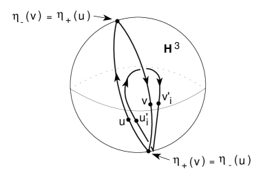
Since $[z,u_{i}]$ is contained in $\widetilde{P}^{\prime}$, it is a $K$-quasigeodesic by lemma 3.3. Since $\tau(z,u_{i})\rightarrow+\infty$, it then follows that $d(z,u_{i})\rightarrow+\infty$, so $d(h_{i}(z),h_{i}(u_{i}))\rightarrow+\infty$. Hence up to taking a further subsequence we may assume that $h_{i}(z)$ converges to some point in $S^{2}_{\infty}$. Since $\tau(h_{i}(z),h_{i}(u_{i}))\rightarrow+\infty$ and $h_{i}(u_{i})\rightarrow u$, lemma 3.7 implies that $h_{i}(z)\rightarrow\eta_{-}(u)$. In addition since $h_{i}(z)\cdot[0,+\infty)$ contains $h_{i}(u_{i})\rightarrow u\in\mbox{$\widetilde{M}$}$ and $h_{i}(u_{i})=h_{i}(z)\cdot r_{i}$ with $r_{i}\rightarrow+\infty$, it follows that every point in $u\cdot\mbox{${\bf R}$}$ is obtained as a limit of points $q_{i}\in h_{i}(z)\cdot[0,+\infty)$. Since $\pi^{-1}(P^{\prime})$ is a closed set in $\widetilde{M}$, this shows that $\pi(u\cdot\mbox{${\bf R}$})$ is contained in $P^{\prime}$ and therefore $u\cdot\mbox{${\bf R}$}$ is a $K$-quasigeodesic. In the same way $h_{i}(y)\rightarrow\eta_{+}(v)$ and $v\cdot\mbox{${\bf R}$}$ is obtained as a limit of $h_{i}(y)\cdot(-\infty,0]$, hence $v\cdot\mbox{${\bf R}$}$ is also a $K$-quasigeodesic, see fig. 5.

Figure 5. Identification of ideal points in an orbit produces two quasigeodesic orbits with same pair of ideal points.

As $d(h_{i}(z),h_{i}(y))$ is a constant, it follows that $\eta_{+}(v)=\eta_{-}(u)$. Since both $v\cdot\mbox{${\bf R}$}$ and $u\cdot\mbox{${\bf R}$}$ are $K$-quasigeodesics, this equality implies that $u$ and $v$ are not in the same flow line of $\widetilde{\Phi}$. But for each $i$, $h_{i}(v_{i})$ and $h_{i}(u_{i})$ are in the same orbit of $\widetilde{\Phi}$, $h_{i}(v_{i})\rightarrow v$, and $h_{i}(u_{i})\rightarrow u$. This contradicts the Hausdorff orbit space condition. We conclude that $\gamma_{0}$ and $\gamma_{1}$ do not have the same ideal point.

Case 2 — $x\cdot{\bf R}$ intersects $\pi^{-1}(S)$ infinitely many times.

Then there is a sequence $E_{1}<\cdots<E_{J_{0}}\in{\mathcal{E}}$ such that $x\cdot{\bf R}$ intersects each, and by lemma 3.4 we have $\sigma^{b}(E_{1})\cap\sigma^{f}(E_{J_{0}})=\emptyset$. But $\eta_{-}(x)\in\sigma^{b}(E_{1})$ and $\eta_{+}(x)\in\sigma^{f}(E_{J_{0}})$ so $\eta_{-}(x)\neq\eta_{+}(x)$. ∎

Finally we prove property (c) of 1.4.

Proposition 3.9.

(continuity of extension) The map $\eta_{+}:\widetilde{\Omega}\rightarrow\mbox{$S^{2}_{\infty}$}$ is continuous and similarly for $\eta_{-}$.

Proof.

We only consider $\eta_{+}$.

Case 1 — $x\cdot[0,+\infty)$ intersects $\pi^{-1}(S)$ infinitely often.

Let $E_{1}<E_{2}<\cdots$ be the elements of $\mathcal{E}$ that $x\cdot[0,+\infty)$ intersects. From lemma 3.5, $\bigcap_{i\in{\bf N}}\sigma^{f}(E_{i})$ is a single point $p$ in $\partial_{\infty}\widetilde{P}$. Since $\sigma^{f}(E_{i})\cap\partial_{\infty}\widetilde{P}$ is a decreasing sequence of compact sets in $\partial_{\infty}\widetilde{P}$, then for each $\delta>0$, there is $i_{0}$ so that $\forall i>i_{0}$, the diameter of $\sigma^{f}(E_{i})\cap\partial_{\infty}\widetilde{P}<\delta$. If $z$ is sufficiently near $x$ then $z\cdot[0,+\infty)$ will intersect $E_{i_{0}}$ therefore $\eta_{+}(z)\in\sigma^{f}(E_{i})\cap\partial_{\infty}\widetilde{P}$. Hence the distance from $\eta_{+}(z)$ to $\eta_{+}(x)$ $<\delta$. This implies that $\eta_{+}$ is continuous at $x$.

Case 2 — $x\cdot[0,+\infty)$ has finite intersection with $\pi^{-1}(S)$.

There is $s_{1}\geq 0$ with $x\cdot[s_{1},+\infty)\cap\pi^{-1}(S)=\emptyset$. Let $x^{\prime}=x\cdot s_{1}$. Since

$$x_{i}\rightarrow x\ \ \Longleftrightarrow\ \ x_{i}\cdot s_{1}\rightarrow x^{\prime},$$

we may assume that $x\cdot[0,+\infty)\cap\pi^{-1}(S)=\emptyset$. Consider a sequence $x_{i}\to x$, and let

$$m_{i}=\bigl{|}x_{i}\cdot[0,+\infty)\cap\pi^{-1}(S)\bigr{|}$$

where $\bigl{|}V\bigr{|}$ denotes cardinality of $V$. Passing to a subsequence, either $m_{i}$ takes a constant value $\leq J_{0}$ for all $i$, or $m_{i}>J_{0}$ for all $i$.

Case 2.1 — $m_{i}=0$ for all $i$.

We may assume all $\gamma_{i}=x_{i}\cdot[0,+\infty)$ and $\gamma_{0}=x\cdot[0,+\infty)$ are in the $\delta_{1}$-neighborhood of $\Omega$. By lemma 3.3, $\gamma_{0}$ and each $\gamma_{i}$ are $K$-quasigeodesic. The proof in this case is finished by lemma 3.7.

Before addressing the case $m_{i}>0$ we need the following lemma.

Lemma 3.10.

Suppose $m_{i}\geq j-1$ for all $i$. Let $v_{i}$ be the $j$-th intersection of $x_{i}~{}\cdot[0,+\infty)$ with $\pi^{-1}(S)$, if it exists, otherwise let $v_{i}=\eta_{+}(x_{i})$. Then $v_{i}$ converges to $\eta_{+}(x)$ in $\widetilde{P}\cup\partial_{\infty}\widetilde{P}$.

Proof.

First suppose $j=1$, and let $v_{i}=x_{i}\cdot t_{i}$ with $t_{i}\in[0,+\infty]$. By lemma 3.3 the segments or rays $[x_{i},v_{i})$ are all $K$-quasigeodesics. In addition $t_{i}\rightarrow+\infty$, since $x\cdot[0,+\infty)\cap\pi^{-1}(S)=\emptyset$ and $x_{i}\rightarrow x$. By lemma 3.7 we conclude that $z_{i}\rightarrow\eta_{+}(x)$.

Figure 6. Successive intersections with ${\mathcal{E}}$.

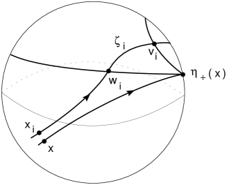
Suppose now that $m_{i}\geq j-1$ for all $i$, and let $w_{i}$ be the $(j-1)$-th intersection. We assume by induction that $w_{i}\to\eta_{+}(x)$. Let $\zeta_{i}=[w_{i},v_{i}]$, so each $\zeta_{i}$ is a $K$-quasigeodesic, see fig. 6. If $\zeta_{i}$ is not escaping compact sets in $\widetilde{P}$, then passing to a subsequence $\zeta_{i}$ accumulates on some $u\in\widetilde{P}$, leading to a contradiction as follows: if $u\in x\cdot\mbox{${\bf R}$}$, then since each $\zeta_{i}-\{w_{i}\}$ is separated from $x$ by at least one element of ${\mathcal{E}}$, this would imply that $x\cdot\mbox{${\bf R}$}_{+}$ has to intersect ${\mathcal{E}}$ contradiction. In the other case, $x$ and $u$ are not on the same flow line, contradicting the Hausdorff orbit space condition.

The paths $\zeta_{i}$ therefore escape to infinity in $\widetilde{P}$. These paths are $K$-quasigeodesics, so their diameters are shrinking to zero in a topological metric on $\widetilde{P}\cup\partial_{\infty}\widetilde{P}$. Since $w_{i}\rightarrow\eta_{+}(x)$ it then follows that $v_{i}\rightarrow\eta_{+}(x)$. Induction now completes the proof of the lemma. ∎

Case 2.2 — $m_{i}=m$ is a constant with $0<m\leq J_{0}$.

Applying lemma 3.10 with $j=m-1$ it follows that $\eta_{+}(x_{i})\to\eta_{+}(x)$.

Case 2.3 — $m_{i}>J_{0}$ for every $i$.

Let $y_{i}$ be the corresponding $(J_{0}+1)$-th intersection. Then $y_{i}\rightarrow\eta_{+}(x)$. Let $C_{i}\in{\mathcal{E}}$ be the lift of $S$ containing $y_{i}$.

If there is an infinite subsequence $i_{l}$ with $C_{i_{l}}=C$ for all $l$, then because $z_{i_{l}}\rightarrow\eta_{+}(x)$, it follows that $\eta_{+}(x)\in\partial_{\infty}C$. But for any $i$, the flow line through $x_{i}$ intersects a sequence $E_{1}<\cdots<E_{J_{0}}\in\mathcal{E}$ before intersecting $C_{i}$. Since $x\cdot[0,+\infty)\subset\sigma^{b}E_{1}$ then $\eta_{+}(x)\in\sigma^{b}E_{1}$, but also $\eta_{+}(x)\in\partial_{\infty}C\subset\sigma^{f}E_{J_{0}}$, and therefore $\sigma^{b}E_{1}\cap\sigma^{f}E_{J_{0}}\neq\emptyset$ contradicting lemma 3.4. We may therefore assume up to taking a further subsequence that all $C_{i}$ are distinct from each other.

Note that there is $E_{0}\in\mathcal{E}$ such that $E_{0}<C_{i}$ for all $i$; take any $E_{0}$ so that $x\in\operatorname{Fr}(E_{0})$. Applying lemma 3.5, there is a subsequence $i_{l}$ so that that $\sigma^{f}C_{i_{l}}$ approaches a single point of $\partial_{\infty}P$ in the Hausdorff topology. This point must be $\eta_{+}(x)$, since $z_{i_{l}}\in\sigma^{f}(C_{i_{l}})$ and $z_{i_{l}}\to\eta_{+}(x)$. Therefore the sequence $\eta_{+}(x_{i_{l}})\in\sigma^{f}(C_{i_{l}})$ approaches $\eta_{+}(x)$.

The arguments of cases 2.1, 2.2 and 2.3, show that given any sequence $y_{i}\rightarrow x$, there is always a subsequence $y_{i_{l}}$ for which $\eta_{+}(y_{i_{l}})\rightarrow\eta_{+}(x)$. This implies that the original sequence $\eta_{+}(y_{i})\rightarrow\eta_{+}(x)$. This finally finishes the proof of proposition 3.9. ∎

Propositions 3.6, 3.8 and 3.9 show that orbits in $\Omega_{n+1}$ satisfy conditions (a,b,c) of theorem 1.4 as orbits in $\widetilde{P}\cup\partial_{\infty}\widetilde{P}$. Since $\widetilde{P}\cup\partial_{\infty}\widetilde{P}$ embeds continuously in $\mbox{${\bf H}^{3}$}\cup\mbox{$S^{2}_{\infty}$}$, it follows that they also satisfy these conditions as seen in $\mbox{${\bf H}^{3}$}\cup\mbox{$S^{2}_{\infty}$}$. Theorem 1.4 then implies that orbits of $\widetilde{\Phi}$ in $\widetilde{P}$ are uniformly quasigeodesic in ${\bf H}^{3}$ (hence also in $\widetilde{P}$). Induction now finishes the proof of theorem $A$.

Remark:  In this article we use the inductive step of this section to study flows transverse to Reebless finite depth foliations. By Novikov’s theorem [No], $\Phi$ satisfies the $\epsilon,T$-cycles condition, hence lemma 1.3 can be applied, simplifying the proof of case 1 in proposition 3.8. However, the inductive proof we give in this section has more general hypothesis, namely: (1) $\widetilde{\Phi}$ has Hausdorff orbit space, (2) $\Phi$ is well adapted to a partial sutured manifold hierarchy, that is, the smallest sutured manifold in the hierarchy, call it $P$ may not be a product sutured manifold; and (3) orbits entirely contained in $P$ are uniform quasigeodesics. There may be flows satisfying these properties, which are not transverse to finite depth foliations.

4. Quasigeodesic pseudo-Anosov flows

Pseudo-Anosov flows are a generalization of suspension flows of pseudo-Anosov surface homeomorphisms. These flows behave much like Anosov flows, but they have finitely many singular orbits with a prescribed behavior. In order to define pseudo-Anosov flows, first we recall singularities of pseudo-Anosov surface homeomorphisms.

Given $n\geq 2$, the quadratic differential $z^{n-2}dz^{2}$ on the complex plane ${\bf C}$ (see [St] for quadratic differentials) has a horizontal singular foliation $f^{u}$ with transverse measure $\mu^{u}$, and a vertical singular foliation $f^{s}$ with transverse measure $\mu^{s}$. These foliations have $n$-pronged singularities at the origin, and are regular and transverse to each other at every other point of ${\bf C}$. Given $\lambda>1$, there is a map $\psi\colon{\bf C}\to{\bf C}$ which takes $f^{u}$ and $f^{s}$ to themselves, preserving the singular leaves, stretching the leaves of $f^{u}$ and compressing the leaves of $f^{s}$ by the factor $\lambda$. Let $R_{\theta}$ be the homeomorphism $z\to e^{2\pi\theta}z$ of ${\bf C}$. If $0\leq k<n$ the map $R_{k/n}\circ\psi$ has a unique fixed point at the origin, and this defines the local model for a pseudohyperbolic fixed point, with $n$-prongs and with rotation $k$. Let $d_{\bf E}$ be the singular Euclidean metric on ${\bf C}$ associated to the quadratic differential $z^{n-2}dz^{2}$, given by

$$d_{\bf E}^{2}=\mu_{u}^{2}+\mu_{s}^{2}$$

Note that

$$(R_{k/n}\circ\psi)^{*}d_{\bf E}^{2}=\lambda^{-2}\mu_{u}^{2}+\lambda^{2}\mu_{s}^{2}$$

Now consider the mapping torus $N={\bf C}\times{\bf R}/(z,r+1)\sim(R_{k/n}\circ\psi(z),r)$, with suspension flow $\Psi$ arising from the flow in the ${\bf R}$ direction on ${\bf C}\times{\bf R}$. The suspension of the origin defines a periodic orbit $\gamma$ in $N$, and we say that $(N,\gamma)$ is the local model for a pseudohyperbolic periodic orbit, with $n$ prongs and with rotation $k$. The suspension of the foliations $f^{u},f^{s}$ define 2-dimensional foliations on $N$, singular along $\gamma$, called the local weak unstable and stable foliations. Note that there is a singular Riemannian metric $ds$ on ${\bf C}\times{\bf R}$ that is preserved by the gluing homeomorphism $(z,r+1)\sim(R_{k/n}\circ\psi(z),r)$, given by the formula

$$ds^{2}=\lambda^{-2t}\mu_{u}^{2}+\lambda^{2t}\mu_{s}^{2}+dt^{s}$$

The metric $ds$ descends to a metric on $N$ denoted $ds_{N}$.

Let $\Phi$ be a flow on a closed, oriented 3-manifold $M$. We say that $\Phi$ is a pseudo-Anosov flow if the following are satisfied:

• For each $x\in M$, the flow line $t\to\Phi(x,t)$ is $C^{1}$, and the tangent vector bundle $D_{t}\Phi$ is $C^{0}$.

• There is a finite number of periodic orbits $\{\gamma_{i}\}$, called singular orbits, such that the flow is smooth off of the singular orbits.

• Each singular orbit $\gamma_{i}$ is locally modelled on a pseudo-hyperbolic periodic orbit. More precisely, there exist $n,k$ with $n\geq 3$ and $0\leq k<n$, such that if $(N,\gamma)$ is the local model for an pseudo-hyperbolic periodic orbit with $n$ prongs and with rotation $k$, then there are neighborhoods $U$ of $\gamma$ in $N$ and $U_{i}$ of $\gamma_{i}$ in $M$, and a diffeomorphism $f\colon U\to U_{i}$, such that $f$ takes orbits of the semiflow $R_{k/n}\circ\psi\bigm{|}U$ to orbits of $\Phi\bigm{|}U_{i}$.

• There exists a path metric $d_{M}$ on $M$, such that $d_{M}$ is a smooth Riemannian metric off of the singular orbits, and for a neighborhood $U_{i}$ of a singular orbit $\gamma_{i}$ as above, the derivative of the map $f\colon(U-\gamma)\to(U_{i}-\gamma_{i})$ has bounded norm, where the norm is measured using the metrics $ds_{N}$ on $U$ and $d_{M}$ on $U_{i}$.

• On $M-\bigcup\gamma_{i}$, there is a continuous splitting of the tangent bundle into three 1-dimensional line bundles $E^{u}\oplus E^{s}\oplus T\Phi$, each invariant under $\Phi$, such that $T\Phi$ is tangent to flow lines, and for some constants $\nu>1,\theta>1$ we have

  1. If $v\in E^{u}$ then $|D\Phi_{t}(v)|\leq\theta\nu^{t}|v|$ for $t<0$

  2. If $v\in E^{s}$ then $|D\Phi_{t}(v)|\leq\theta\nu^{-t}|v|$ for $t>0$

  where norms of tangent vectors are measured using the metric $d_{M}$.

With the definition formulated in this manner, the entire theory of Anosov flows can be mimicked for pseudo-Anosov flows. In particular, a pseudo-Anosov flow $\Phi$ has a 2-dimensional weak unstable foliation ${\mathcal{F}}^{u}$ tangent to $E^{u}\oplus T\Phi$ away from the singular orbits, and a 2-dimensional weak stable foliation ${\mathcal{F}}^{s}$ tangent to $E^{s}\oplus T\Phi$. These foliations are singular along the singular orbits of $\Phi$, and regular everywhere else. In the neighborhood $U_{i}$ of an $n$-pronged singular orbit $\gamma_{i}$, the images of ${\mathcal{F}}^{s}$ and ${\mathcal{F}}^{u}$ in the model manifold $N$ are identical with the local weak stable and unstable foliations.

The restriction of ${\mathcal{F}}^{s}$ to $M-$ (singular orbits) defines a true foliation; a complete leaf of this foliation is called a nonsingular leaf of ${\mathcal{F}}^{s}$; an incomplete leaf may be completed by adding a singular orbit $\gamma$ of $\Phi$, and the result is called a singular leaf of ${\mathcal{F}}^{s}$ abutting $\gamma$. Singular and nonsingular leaves of ${\mathcal{F}}^{u}$ are similarly defined. The bare term “leaf” means either a nonsingular or a singular leaf. For some small neighborhood $W$ of any point $x$ lying on a singular orbit $\gamma$, the singular leaves of ${\mathcal{F}}^{s}$ divide $W$ into $n$ sectors, each sector parameterized by $D^{2}\times I$, so that the restriction of ${\mathcal{F}}^{s}$ to the sector agrees with the foliation by level discs $D^{2}\times t$; and similarly for ${\mathcal{F}}^{u}$. All the terms defined here apply as well to the lifted singular foliations $\mbox{${\widetilde{\mathcal{F}}}^{s}$},\mbox{${\widetilde{\mathcal{F}}}^{u}$}$ in $\widetilde{M}$.

Proposition 4.1.

If $\Phi$ is a pseudo-Anosov flow in $M^{3}$ then the orbit space $\mathcal{O}$ of $\widetilde{\Phi}$ is homeomorphic to $\mbox{${\bf R}$}^{2}$.

Proof.

Let $\mbox{${\mathcal{F}}^{s}$},\mbox{${\mathcal{F}}^{u}$}$ be the singular stable and unstable foliations of $\Phi$. A short embedded path $\alpha$ is a quasi-transversal of ${\mathcal{F}}^{s}$ if one of the following happens: either $\alpha$ is transverse to ${\mathcal{F}}^{s}$; or there is a singular orbit $\gamma$ and $x\in\operatorname{int}(\alpha)\cap\gamma$ such that the closure of each half of $\alpha-x$ either is transverse to ${\mathcal{F}}^{s}$ or lies on a singular leaf of ${\mathcal{F}}^{s}$, and the two halves do not both lie in the closure of any sector of ${\mathcal{F}}^{s}$ at $x$. Quasitransversals of ${\mathcal{F}}^{u}$ are similarly defined. We need the following facts about $\Phi$, ${\mathcal{F}}^{s}$ and ${\mathcal{F}}^{u}$.

1. Each periodic orbit of $\Phi$ is homotopically nontrivial.

2. A quasitransversal $\rho$ of ${\mathcal{F}}^{u}$ is not path homotopic into a leaf of ${\mathcal{F}}^{u}$; and similary for ${\mathcal{F}}^{s}$.

3. The inclusion map of every leaf of ${\widetilde{\mathcal{F}}}^{s}$ or ${\widetilde{\mathcal{F}}}^{u}$ into $\widetilde{M}$ is proper.

These facts are proved using the theory of essential laminations [Ga-Oe]; we give the argument for ${\mathcal{F}}^{s}$. Split ${\mathcal{F}}^{s}$ along singular leaves to produce a lamination ${\mathcal{L}}^{s}$. There is one complementary component $T_{\gamma}$ of ${\mathcal{L}}^{s}$ for each singular orbit $\gamma$ of $\Phi$, and if $\widehat{T}_{\gamma}$ is the metric completion of $T_{\gamma}$ then $\widehat{T}_{\gamma}$ is homeomorphic to a solid torus with an $(n,k)$ torus knot removed from the boundary, where $\gamma$ has $n$ prongs and rotation $k$. Since $n\geq 3$ for all $\gamma$ it follows that ${\mathcal{L}}^{s}$ is an essential lamination. There is a map $f\colon M\to M$ homotopic to the identity taking ${\mathcal{L}}^{s}$ onto $\mbox{$\mathcal{F}$}^{s}$, taking each leaf of ${\mathcal{L}}^{s}$ not on the boundary of some $T_{\gamma}$ homeomorphically onto a non-singular leaf of ${\mathcal{F}}^{s}$, and taking each leaf on the boundary of each $T_{\gamma}$ onto a union of singular leaves abutting $\gamma$. Given a leaf $L\subset\partial T_{\gamma}$ if gcd$(n,k)\neq 1$ then $L$ is mapped onto a union of two singular leaves and the map is 1-1 off of $\gamma$; and if gcd$(n,k)=1$ then $L$ maps onto one singular leaf and the map is 2-1 off of $\gamma$; in either case, $f^{-1}(\gamma)\cap L$ is a core curve of the annulus $L$.

Properties (1–3) follow from results of [Ga-Oe]. Property (1) follows because each periodic orbit of $\Phi$ is homotopically nontrivial in a leaf of ${\mathcal{F}}^{s}$, and because leaves of ${\mathcal{L}}^{s}$ are $\pi_{1}$-injective. Property (2) follows because if $\rho^{\prime}$ is a path transverse to ${\mathcal{L}}^{s}$, and if the closure of each component of $\rho^{\prime}-\mbox{${\mathcal{L}}^{s}$}$ is not path homotopic into a leaf of ${\mathcal{L}}^{s}$, then $\rho^{\prime}$ is not path homotopic into a leaf of ${\mathcal{L}}^{s}$. Property (3) follows because leaves of $\widetilde{\mathcal{L}}^{s}$ and $\widetilde{\mathcal{L}}^{u}$ include properly in $\widetilde{M}$.

In order to prove the proposition, the key facts to prove are that $\mathcal{O}$ is a two dimensional manifold and that it is Hausdorff.

Suppose there are $\epsilon,T$-cycles of $\Phi$ for $\epsilon$ arbitrarily small and $T$ arbitrarily big. We can then choose $x_{i}\rightarrow x\in\mbox{$\widetilde{M}$}$ and $t_{i}\to+\infty$ so that $y_{i}=x_{i}\cdot t_{i}\to x$. Let $\alpha_{i}=x_{i}\cdot[0,t_{i}]$. If $x_{i},y_{i}$ are in the same local orbit of $\widetilde{\Phi}$ near $x$, then $\alpha_{i}$ can be easily completed to a closed orbit, contradicting property (1) above. If the endpoints of $\alpha_{i}$ are not in the same local orbit and $\epsilon$ is sufficiently small, then the endpoints of $\alpha_{i}$ may be joined by a path $\beta$ which is a quasi-transversal to either ${\widetilde{\mathcal{F}}}^{s}$ or ${\widetilde{\mathcal{F}}}^{u}$; but $\beta$ is path homotopic to $\alpha_{i}$, contradicting property (2) above.

This implies that $\mathcal{O}$ is locally $2$-dimensional. We next prove that it is Hausdorff. The proof given for Anosov flows in [Fe1] goes through almost verbatim, with slight changes to take pseudo-Anosov behavior into account, or we may proceed as follows.

Let $x_{i}\rightarrow x$, $y_{i}=x_{i}\cdot t_{i}\rightarrow y$ in $\widetilde{M}$. We first want to show that $t_{i}$ is bounded. Assume then up to taking a subsequence that $t_{i}\rightarrow+\infty$. If $x$ lies on a singular orbit $\gamma$ of $\Phi$, pass to a subsequence so that $x_{i}$ lies in a single sector of ${\widetilde{\mathcal{F}}}^{s}$ near $x$. Now vary $x_{i}$ to nearby $z_{i}$, so that $z_{i}\rightarrow x$, $z_{i}\in\mbox{$\widetilde{W}^{s}$}(x_{i})\cap\mbox{$\widetilde{W}^{u}$}(x)$. Since flow lines in the stable foliation converge together exponentially it follows that there are $s_{i}\rightarrow+\infty$ with $w_{i}=z_{i}\cdot s_{i}\rightarrow y$. The sequence $z_{i}$ forms a bounded subset of a leaf $L$ of $\mbox{$\widetilde{W}^{u}$}(x)$, and hence the sequence $z_{i}\cdot s_{i}$ leaves every compact subset of $L$, because flow lines are properly embedded in the leaf $L$ — the flow induces a product structure in $L$. But by (3) above the inclusion map $L\hookrightarrow\mbox{$\widetilde{M}$}$ is proper, contradicting that $z_{i}\cdot s_{i}$ converges in $\widetilde{M}$. This contradiction shows that the $t_{i}$ are bounded.

As the $t_{i}$ are bounded, we may assume up to subsequence that $t_{i}\rightarrow t_{0}$. Then $y_{i}\rightarrow x\cdot t_{0}=y$. This shows that $\mathcal{O}$ is Hausdorff and it follows that it is homeomorphic to $\mbox{${\bf R}$}^{2}$. ∎

Given any closed, irreducible, orientable $3$-manifold $M$ with $H_{2}(M)\not=0$, Gabai [Ga1] constructed many finite depth foliations in $M$: for any $\zeta\not=0$ in $H_{2}(M)$ there is a taut, finite depth foliation $\mathcal{F}$ in $M$ so that the compact leaves of $\mathcal{F}$ represent $\zeta$.

If in addition $M$ is atoroidal, then Mosher [Mo4] constructed pseudo-Anosov flows in $M$ which are almost tranverse to $\mathcal{F}$. These flows become transverse to $\mathcal{F}$ after blow up of finitely many singular orbits $\gamma_{i},1\leq i\leq i_{0}$ of $\Phi$. The blown up flow is denoted by $\Phi^{b}$. The blow up transforms the orbit $\gamma_{i}$ into $Z_{i}=(T_{i}\times[0,1])/f$, where $T_{i}$ is a finite simplicial tree, and $f$ is a homeomorphism of $T_{i}\times\{1\}$ to $T_{i}\times\{0\}$ which sends edges to edges. Each edge $E$ of $T_{i}$ eventually returns to itself, producing an annulus $A$ in $Z_{i}$. The flow in $A$ is as follows: the boundary consists of two orbits coherently oriented, and the interior orbits spiral from one boundary circle to the other without forming a two dimensional Reeb component. Clearly there is a global section to $\Phi^{b}$ restricted to $Z_{i}$. The flow $\Phi^{b}$ is transverse to $\mathcal{F}$.

In addition $\Phi^{b}$ is semiconjugate to $\Phi$: there is a continuous map $q\colon M\to M$, so that

• $q$ is homotopic to the identity,

• $q$ takes orbits of $\Phi^{b}$ to orbits of $\Phi$ preserving orientation,

• $q$ is $C^{1}$ along orbits of $\Phi^{b}$,

• $q$ is one to one except in $\cup_{1\leq i\leq i_{0}}Z_{i}$,

• $q(Z_{i})=\gamma_{i}$.

Proposition 4.2.

The orbit space $\mbox{$\mathcal{O}$}^{b}$ of $\mbox{$\widetilde{\Phi}$}^{b}$ is homeomorphic to $\mbox{${\bf R}$}^{2}$.

Proof.

Since $\Phi^{b}$ is transverse to $\mathcal{F}$, then if $\epsilon>0$ is very small and $T>0$ very large, it follows that an $\epsilon,T$ cycle can be perturbed to be transverse to $\mathcal{F}$, hence it is not null homotopic by Novikov’s theorem [No]. This shows that $\mbox{$\mathcal{O}$}^{b}$ is locally two dimensional. We now show that $\mbox{$\mathcal{O}$}^{b}$ is Hausdorff.

Lift $q$ to a map $\widetilde{q}\colon\mbox{$\widetilde{M}$}\rightarrow\mbox{$\widetilde{M}$}$, which is boundedly homotopic to the identity map. Let $\tau(x,y)$ be the difference in flow parameter between $x,y$ on the same flow line of $\widetilde{\Phi}$, and let $\tau^{b}(x,y)$ be similarly defined for $\mbox{$\widetilde{\Phi}$}^{b}$.

Claim — There are $m_{0},m_{1}>0$ so that if $x,y$ are in the same flow line of $\mbox{$\widetilde{\Phi}$}^{b}$, then $m_{0}\tau^{b}(x,y)<\tau(\tilde{q}(x),\tilde{q}(y))<m_{1}\tau^{b}(x,y)$.

Given $z\in M$, let $g(z)$ be the derivative at $z$ of $q$ restricted to the flow line through $z$. Then since $g(z)$ is continuous and positive and $M$ compact, there are $m_{0}$ and $m_{1}>0$ which are the maxima and minima of $g$ in $M$. The claim follows.

Let now $x_{i}\in\mbox{$\widetilde{M}$},y_{i}=\mbox{$\widetilde{\Phi}$}^{b}_{t_{i}}(x_{i})$ so that $y_{i}\rightarrow y$ and $x_{i}\rightarrow x$. Then $\tilde{q}(x_{i})\rightarrow\tilde{q}(x)$ and $\tilde{q}(y_{i})\rightarrow\tilde{q}(y)$. Since $\Phi$ is pseudo-Anosov, the previous proposition shows that the orbit space $\mathcal{O}$ of $\widetilde{\Phi}$ is Hausdorff, hence $\tilde{q}(y)=\mbox{$\widetilde{\Phi}$}_{s}(\tilde{q}(x))$. Since $\mathcal{O}$ is homeomorphic to $\mbox{${\bf R}$}^{2}$, it follows that $\tilde{q}(y_{i})=\mbox{$\widetilde{\Phi}$}_{s_{i}}(\tilde{q}(x_{i}))$ where $s_{i}\rightarrow s$.

Partitioning $s_{i}$ into a uniformly bounded number of subsegments of length $\leq 1$, and using the claim above, it follows that $y_{i}=\mbox{$\widetilde{\Phi}$}^{b}_{r_{i}}(x_{i})$ where $r_{i}$ is uniformly bounded. Up to taking a subsequence, assume that $r_{i}$ converges to some $r$, and hence $y_{i}\rightarrow\mbox{$\widetilde{\Phi}$}^{b}_{r}(x)$. Consequently $y=\mbox{$\widetilde{\Phi}$}^{b}_{r}(x)$. This shows that $\mbox{$\mathcal{O}$}^{b}$ is Hausdorff. It follows that $\mbox{$\mathcal{O}$}^{b}$ is homeomorphic to $\mbox{${\bf R}$}^{2}$. ∎

Now we prove the main theorem:

Main theorem  Let $M^{3}$ be closed, orientable, irreducible with non zero second betti number. Let $\zeta\not=0\in H_{2}(M)$ and $\mathcal{F}$ be a taut finite depth foliation with compact leaves representing $\zeta$. Let $\Phi$ be a pseudo-Anosov flow which is almost transverse to $\mathcal{F}$. Then $\Phi$ is quasigeodesic.

Proof.

By the previous proposition the flow $\widetilde{\Phi}^{b}$ on $\widetilde{M}$ has Hausdorff orbit space.

Suppose first that $\mathcal{F}$ has a compact leaf which is not a fiber. Then $\Phi^{b}$ is quasigeodesic by theorem A. The semiconjugacy $\tilde{q}$ from $\widetilde{\Phi}^{b}$ to $\widetilde{\Phi}$ moves points a uniformly bounded distance in $\widetilde{M}$. Since there is also a bound on how much the map $\tilde{q}$ expands the lengths of flow lines (given by the claim in the previous proposition), it follows that flow lines of $\widetilde{\Phi}$ are uniform quasigeodesics.

Now suppose that each compact leaf of $\mathcal{F}$ is a fiber. If $\mathcal{F}$ is a fibration over the circle, then $\Phi^{b}$ is quasigeodesic by [Ze], and the arguments of the previous paragraph show that $\Phi$ is quasigeodesic.

Suppose $\mathcal{F}$ is not a fibration over the circle. We claim that $\mathcal{F}$ can be replaced by another finite depth foliation of smaller depth that is still transverse to $\Phi^{b}$; continuing by induction, eventually $\Phi^{b}$ is transverse to a fibration over the circle, and we are done.

We sketch a proof of the claim. Let $\mathcal{F}$ have depth $n$. Note that each component of $\mbox{$\mathcal{F}$}-\mbox{$\mathcal{F}$}^{0}$ is homeomorphic to the product of a depth 0 leaf crossed with an interval; similarly each component of $\mbox{$\mathcal{F}$}-\mbox{$\mathcal{F}$}^{k}$ is homeomorphic to the product of a depth $k$ leaf crossed with an interval. Note also that the restriction of $\mathcal{F}$ to a component of $\mbox{$\mathcal{F}$}-\mbox{$\mathcal{F}$}^{n-1}$ is a fibration over the circle with fiber a depth $n$ leaf $L$. It follows that if $f\colon L\to L$ is the first return map of $\Phi^{b}$, then there is a translation map $g\colon L\to L$, i.e. a map which generates a properly discontinuous, free action of ${\bf Z}$, such that $f$ is isotopic to $g$ by a compactly supported isotopy. Any compact subset of $L$ invariant under $f$ is contained in the support of the isotopy from $f$ to $g$, and hence there is a maximal compact invariant set $C$ of $f$. Using the fact that $\Phi^{b}$ is a blown up pseudo-Anosov flow, the set $C$ is nonempty if and only if $f$ has periodic points. Moreover, any periodic points are non-removable in the proper isotopy class of $f$; the proof given for pseudo-Anosov surface homeomorphisms in [Bi-Ki] works just as well in the present context. Since $g$ has no periodic points, it follows that $C=\emptyset$, and therefore $f$ is itself a translation map. The component of $\mbox{$\mathcal{F}$}-\mbox{$\mathcal{F}$}^{n-1}$ containing $L$ may therefore be refoliated by leaves of depth $n-1$, staying transverse to $\Phi^{b}$. Doing this for each component of $\mbox{$\mathcal{F}$}-\mbox{$\mathcal{F}$}^{n-1}$ proves the claim. ∎

References

- [BKS] T. Bedford, M. Keane and C. Series, eds., Ergodic theory, symbolic dynamics, and hyperbolic spaces, Oxford Science Publications (1991).
- [Be-Me] M. Bestvina and J. Mess, The boundary of negatively curved groups, Jour. Amer. Math. Soc. 4 (1991) 469–481.
- [Bi-Ki] J. Birman and M. Kidwell, Fixed points of pseudo-Anosov diffeomorphismsof surfaces, Adv. in Math. 46 (1982) 217–220.
- [Bo] F. Bonahon, Bouts des variétés hyperboliques, Ann. of Math. 124 (1986) 71–158.
- [Cn] R. Canary, Covering theorems for hyperbolic -manifolds, in Proceedings of Low Dimensional Topology, Int. Press, 1994.
- [Ca-Co] J. Cantwell and L. Conlon, Smoothability of proper foliations, Ann. Inst. Fourier Grenoble, 38 (1988) 219–244.
- [Ca] J. Cannon, The combinatorial structure of cocompact discrete hyperbolic groups, Geom. Ded. 16 (1984) 123–148.
- [Ca-Th] J. Cannon and W. Thurston Group invariant peano curves, to appear.
- [Co] C. Conley, Isolated invariant sets and the Morse index, Reg. Conf. Ser. Math., 38, Providence, Am. Math. Soc., (1978).
- [Di] P. Dippolito, Codimension one foliations of closed manifolds, Ann. of Math. 107 (1978) 401–453.
- [Fe1] S. Fenley, Anosov flows in -manifolds, Ann. of Math 139 (1994) 79-115.
- [Fe2] S. Fenley, Quasigeodesic Anosov flows and homotopic properties of flow lines, Jour. Diff. Geom., 41 (1995) 479–516.
- [Fe3] S. Fenley, Global and local properties of limit sets of foliations of quasigeodesic Anosov flows, to appear.
- [Fe4] S. Fenley, Quasi-isometric foliations, Topology 31 (1992) 667–676.
- [Ga1] D. Gabai, Foliations and the topology of 3-manifolds, J. Diff. Geo. 18 (1983) 445–503.
- [Ga2] D. Gabai, Foliations and the topology of 3-manifolds II, J. Diff. Geo. 26 (1987) 461–478.
- [Ga3] D. Gabai, Foliations and the topology of 3-manifolds III, J. Diff. Geo. 26 (1987) 479–536.
- [Ga-Oe] D. Gabai and U. Oertel, Essential laminations and -manifolds, Ann. of Math. 130 (1989) 41–73.
- [Gh-Ha] E. Ghys and P. de la Harpe, eds., Sur les groupes hyperboliques d’aprés Mikhael Gromov, Progress in Math., 83 Birkháuser, 1991.
- [Gr] M. Gromov, Hyperbolic groups, in Essays on group theory, 75–263, Springer, 1987.
- [Ma] B. Maskit, Kleinian groups, Springer Verlag, 1988.
- [Ma] A. Marden, The geometry of finitely generated Kleinian groups, Ann. of Math. 99 (1974) 383–462.
- [Mc-MS] D. McCullough, A. Miller and G. A. Swarup, Uniqueness of cores of noncompact -manifolds, Jour. London Math. Soc. (2) 32 (1985) 548–556.
- [Mi] J. Milnor, A note on curvature and fundamental group, J. Diff. Geo. 2 (1968) 1–7.
- [Mor] J. Morgan, On Thurston’s uniformization theorem for 3 dimensional manifolds, in The Smith conjecture, ed. by J. Morgan and H. Bass, Academic Press, 1984, pp. 37–125.
- [Mo1] L. Mosher, Dynamical systems and the homology norm of a -manifold I. Efficient interesection of surfaces and flows, Duke Math. Jour. 65 (1992) 449–500.
- [Mo2] L. Mosher, Dynamical systems and the homology norm of a -manifold II, Invent. Math. 107 (1992) 243–281.
- [Mo3] L. Mosher, Examples of quasigeodesic flows on hyperbolic -manifolds, in Proceedings of the Ohio State University Research Semester on Low-Dimensional topology, W. de Gruyter, 1992.
- [Mo4] L. Mosher, Laminations and flows transverse to finite depth foliations, in preparation.
- [No] S. P. Novikov, Topology of foliations, Trans. Moscow Math. Soc. 14 (1963) 268–305.
- [St] K. Strebel, Quadratic differentials, Springer Verlag, 1984.
- [Su] P. Susskind, Kleinian groups with intersecting limit sets, J. d’Analyse Mathematique 52 (1989) 26–38.
- [Th1] W. Thurston, The geometry and topology of 3-manifolds, Princeton University Lecture Notes, 1982.
- [Th2] W. Thurston, 3-dimensional manifolds, Kleinian Groups and hyperbolic geometry, Bull. A.M.S.,6 (new series), (1982) 357-381.
- [Ze] A. Zeghib, Sur les feuilletages géodésiques continus des variétés hyperboliques, Inven. Math. 114 (1993) 193–206.