![[Uncaptioned image]](/html/math/9501233/assets/x1.png)
Further Travels with My Ant
Published in modified form: Math. Intelligencer 17 (1995), 48–56 Stony Brook IMS Preprint #1995/1 January 1995
1 Introduction
A recurring theme of this column over the past four years has been what we have referred to as computer-generated mysteries. Examples are sequences defined by simple rational recursions whose terms turn out to be integers with interesting but unexplained divisibility properties, or geometric configurations that are observed to exist although there are no proofs of existence. In most of the examples the reported mysteries have remained unsolved and in some cases may in fact be, in a suitable sense, “unsolvable”. It is therefore gratifying to be able to present in this month’s column an elegant solution of a previously described mystery. An especially pleasing feature of this solution is the fact that the “breakthrough” was made possible by drawing the right picture. Once the picture is drawn it becomes clear what must be proved, after which further study of the pictures gives the clue as to how to construct the proof. It turns out that at one point one needs to use the Jordan curve theorem for a special class of closed curves.
In the paragraphs to follow we shall present an informal but hopefully convincing argument which will require little more of the reader than the careful observation of a collection of pictures.
2 The Story So Far and the Mystery
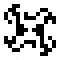
We shall be concerned once again with a certain automaton that has been called an ant. An ant lives in a plane that has been partitioned in the standard way into squares, or, as we shall call them, cells (think of the corners of the cells as the lattice points of the plane). Each cell can be in one of several states, and the respective states of these cells change over the course of time, as the cells are in turn visited by the ant. Before we explain precisely how the ant interacts with its surroundings, it will help to consider a specific example. In the simplest non-trivial version of the ant, originally studied by Chris Langton, there are just two states, which we will call L (for left) and R (for right). We think of the ant as starting on the boundary between two cells, heading in one of the four cardinal compass directions (East or West on the vertical boundaries, and North or South on the horizontal ones). As the ant advances through the cell, it makes a 90 degree turn, turning left in L-cells and right in R-cells, and moves to the boundary of the the neighboring cell. As the ant leaves each cell, it changes the state of the cell, switching L-cells to R-cells, and vice versa. For an informal discussion of this ant see [1], where a number of interesting ant behaviors are observed. For our present purposes we note only the following still unexplained phenomenon: If initially all cells were in the same state, then at various times the ant’s “track” (the set of cells it has visited, together with their current states) is centrally symmetric, that is, the configuration of L- and R-cells has central symmetry. We reproduce here, in Figure 1, the corresponding pictures, where the R-cells are black and the L-cells white; all cells were initially in the L state and the ant started out heading west on the right boundary of the central cell, and about to enter it. These central symmetries stop occurring eventually and after about 10,000 time-units the ant settles into a periodic “highway-building” behavior, heading off to infinity in a southwesterly direction. This phenomenon of “transient symmetry” awaits a satisfying explanation.

In our next episode [2], Jim Propp describes the behavior of the more general -state ants. There are now different states for cells to be in, numbered 1 through , and it is the ant’s internal “programming” which tells it which states to treat as L’s and which states to treat as R’s in choosing which way to turn. We represent this programming by means of a rule-string, a string of L’s and R’s whose -th letter represents the ant’s course of action when it comes to a cell in state ; for instance, the 7-state string LLRRRLR represents an ant that turns left on visiting cells in states 1, 2, and 6 and turns right on visiting cells in states 3, 4, 5, and 7. When an ant comes to an L-cell (a cell in an L-state), it turns left; when it comes to an R-cell, it turns right. When the ant leaves a cell that is in state the cell changes to state (mod ). In this terminology the simple ant has the rule-string LR.
From symmetry considerations it clearly suffices to consider only strings that start with an L. If in the rule-string we replace an L by a 1 and an R by 0 we see that each ant corresponds to a positive integer expressed in base two, so the simple ant is ant 2 and our seven-state ant with “genome” LLRRRLR is ant 98. Propp finds that different ants behave very differently depending on their rule-strings. Some seem to be completely chaotic, while others eventually build highways. The only general statement that can be made is the following
Fundamental Theorem of Myrmecology (Bunimovich-Troubetzkoy):
An ant’s track is always unbounded.
(For a proof see [1]. Note that the attribution given there is incorrect; the proof actually first appeared in [3].)
In this exposition we concentrate on the phenomenon described by Propp as follows.
“Ants 9 and 12 [LRRL and LLRR in our notation] are the truly surprising ones [among ants with rule-strings of length 4]. In each case the the patterns get ever larger, but without ever getting too far away from bilateral symmetry! More specifically, one finds that the ant makes frequent visits to the cell it started from, and when it does, the total configuration quite often has bilateral symmetry.”
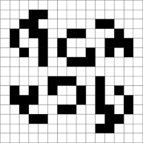
![[Uncaptioned image]](/html/math/9501233/assets/x5.png) Figure 2: The universe of ant 12 at time 16,464.
Figure 2: The universe of ant 12 at time 16,464.
![[Uncaptioned image]](/html/math/9501233/assets/x6.png) Figure 3: The universe of ant 9 at time 38,836.
Figure 3: The universe of ant 9 at time 38,836.
Figures 2 and 3, reproduced from [2], show the track of ant 12 after 16,464 steps and the track of ant 9 after 36,836 steps. The figures use black, white and two shades of grey to indicate the four different states. Propp continues, “To find more ants of this sort we have to move to rule strings of length 6. Here we encounter another mystery: the rule strings that lead to bilaterally symmetric patterns are 33, 39, 48, 51, and 60. Note that all these numbers are divisible by three! Surely this cannot be an accident.” Indeed it is not, as we will presently show.
3 The Picture. Truchet Tiles.
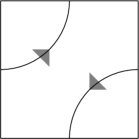
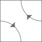
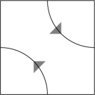
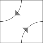
First a preliminary observation. Since an ant turns through a right angle after each move, it follows that its moves are alternately horizontal and vertical. Therefore the cells of the plane split up checkerboard-fashion into two sets: H-cells, which the ant always enters horizontally, from the left or the right, and exits vertically, either at the top or the bottom; and V-cells, which the ant always enters vertically and exits horizontally. Now, a crucial property of a cell is that it is able to change its state and thus change the course of action (left-turn versus right-turn) that the ant will take after its next visit to the cell. The key idea for representing this property, due to Bernd Rümmler, was to actually install schematic “switches” in the cells, in which the orientation of the switch indicates whether the cell is currently an L-state or an R-state. These switches are called Truchet tiles and are illustrated in Figure 4, which shows an H-tile first in its L and then in its R orientation, and Figure 5 which shows the same thing for a V-tile. (An “H-tile” is the Truchet tile associated with an H-cell, and similarly for V-tiles.) Note that switching orientation corresponds to reflecting the tile about either its vertical or horizontal axis.
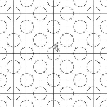
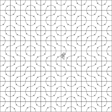
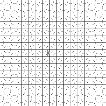
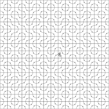
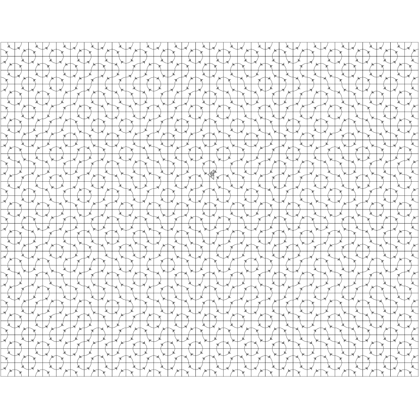
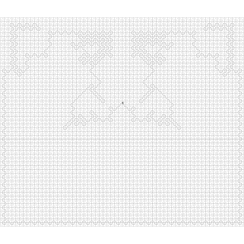
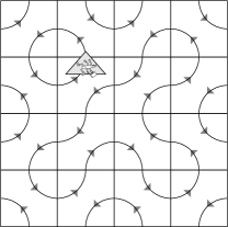
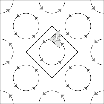
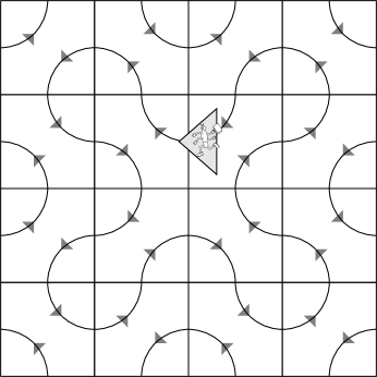
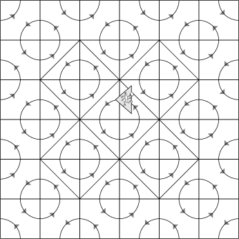
Figure 6 shows the plane paved with Truchet tiles all of which have the L orientation, giving a pattern of disjoint circles: the “initial configuration”. As the ant moves, some of the tiles will switch in accordance with the given rule-string, but it is clear that the pattern will always be made up of a set of disjoint simple closed curves which we shall call Truchet contours. (Infinite contours cannot arise, since at each stage the ant has only switched finitely many of the tiles.) It will be helpful (at least for now) to imagine that the ant actually travels along the Truchet curves themselves, rather than along a lattice-path joining the centers of the cells, and that the ant’s initial position is the midpoint of one of the edges of the central Truchet tile. Figure 7 gives the “Truchet pictures” corresponding to the (transiently) centrally-symmetric configurations of the simple ant given by the earlier Figure 1, while Figures 8 and 9 give Truchet pictures corresponding to the earlier Figures 2 and 3, and manifest the same bilateral symmetry. In all of these pictures the ant has returned to its original location, and of particular interest is the Truchet contour through this point, which we will call the principal contour. Initially, the principal contour is just a circle as are all other contours. In Figure 9 the principal contour has been highlighted.
Now if one knew that each time the ant left its starting location it would stay on the principal contour until it returned once more to its starting location then it would follow that when the ant had completed its tour all the symmetries of the initial state of the universe would be preserved; for whenever a cell was visited its symmetric mate would also be visited.

Unfortunately, an ant will not in general stay on the principal contour, because (as in Figure 10) the contour may pass through some cells twice. This means that when the ant returns to such a cell the orientation of that cell may have switched (indeed this will always be the case for the simple ant studied by Langton), causing the ant to leave the principal contour. However, for the ants listed by Propp one can show that in fact
| The cells that are visited twice by a contour never switch on the first visit. | (1) |
This implies that the ant will engage in a process of repeatedly tracing out bilaterally-symmetric principal contours, resulting in a bilaterally-symmetric universe each time the ant returns to its starting point. Property (1) was first proved by Rümmler for ant 12 and then generalized to the other ants by Troubetzkoy. The argument to follow is a reworking by Propp of those proofs.
4 The Even Run-Length Property and the Augmented Picture
Why do some ant tracks exhibit recurrent bilateral symmetry and others not? Here are the rule-strings for the 4- and 6-state ants of Propp’s article that exhibit recurrent symmetry.
| Ant | Rule-string |
|---|---|
| 9 | LRRL |
| 12 | LLRR |
| 33 | LRRRRL |
| 39 | LRRLLL |
| 48 | LLRRRR |
| 51 | LLRRLL |
| 57 | LLLRRL |
| 60 | LLLLRR |
It is not hard to see what these strings have in common. If we think of them arranged in cyclic rather than linear order then each of them consists of an even number of L’s followed by an even number of R’s. In general we say a rule-string has the even run-length property if in the cyclic order it consists of alternate runs of L’s and R’s of even length, e.g. LRRLLRRRRL. For simplicity in what follows we will consider only the case where the string starts with an even number of L’s (ants 12, 48, 51 and 60), the argument for the other case being similar.
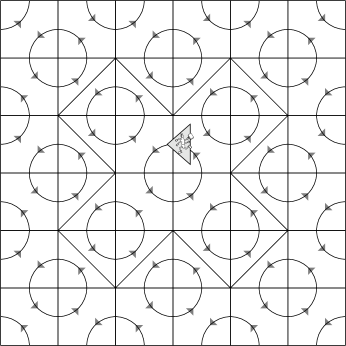
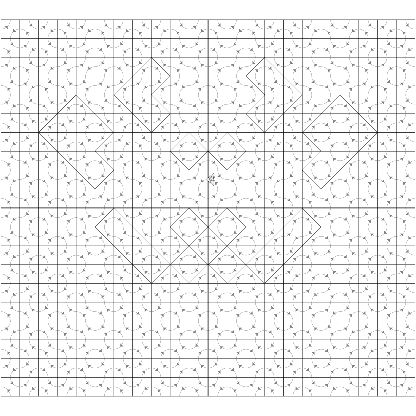
Why does the even run-length property imply recurrence of bilateral symmetry? Here Rümmler has augmented the picture in a manner that can be paraphrased as follows. Let us say that a cell is cold if its state is odd, so that it will not change orientation the next time it is visited (because of the even run-length property), and hot if its state is even, so that it may or may not change orientation the next time it is visited. To complete the picture we make the convention that for hot cells we display not only the Truchet tile but also its diagonal. The diagonals graph is the graph whose edges consist of the diagonals of the hot tiles. Figures 11 and 12 show the diagonals graph of ants 12 and 48 associated with certain instants in time at which the ant has returned to its initial location (hereafter called “home”). Note that these graphs can be quite complicated, breaking up into six components as shown in Figure 12. However, observe a key fact, which we call the even diagonal-degree property:
| All vertices in the diagonals graph have even degree (0, 2, or 4). | (2) |
Lemma 1
Suppose that the ant is at its home position, and that the state of the universe satisfies (2). Then the ant will travel along the principal contour (and return home).
Proof: As was remarked earlier, the only thing we have to worry about is that the principal contour might visit a cell twice, and that this cell might change its orientation after the ant’s first visit. If the twice-visited cell is cold, then the Truchet tile will not change its orientation after the ant’s first visit. What about twice-visited cells that are hot? We will show that such cells do not exist, as a consequence of (2). Let be such a cell, and let be the diagonal of connecting vertices and .
Claim: If is deleted then in the resulting graph the components of and are disjoint.
If we can show this, then the desired contradiction follows, since from (2) the component of (or ) would contain only one vertex of odd degree, contradicting the well-known fact (usually associated with Euler) that a connected graph must always have an even number of vertices of odd degree. (This is sometimes referred to as the handshake theorem, in that it says that the number of people who have shaken hands an odd number of times is even.)


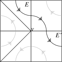
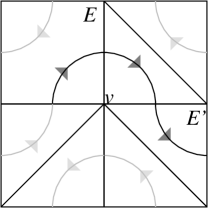
It remains to prove the claim. For this purpose consider the twice-visited tile and its two arcs (quarter circles). Without loss of generality, we assume that is an H-tile. Now color in red the arc in below the diagonal and in addition all succeeding arcs of up to the point where is about to re-enter . Color the remaining arcs blue. The dotted arcs in Figures 13(a) and 14(a) represent the red arcs and the solid arcs represent the blue. Now consider the same picture except that the diagonal of has been deleted and has switched to its other orientation, as shown in Figures 13(b) and 14(b); as before, the arc in below the diagonal should be colored red and the other arc blue. One sees at once that has split into two contours, one all red, the other all blue (this much is a purely combinatorial fact and has nothing to do with the topology of the plane). Now the Jordan curve theorem tells us that each of these non-intersecting contours has an inside and an outside, which can be arranged either as in Figure 13(b) (the non-nested case) or as in Figure 14(b) (the nested case). In either case it is clear that the components of and are disjoint, since both the red contour and blue contour intervene. Combining this with the handshake theorem completes the proof.
Remark: While these last observations can be made rigorous without using the full force of the Jordan curve theorem, there must be some use of the topology of the plane since the analogue of Lemma 1 is not true on the torus.
Finally, we must prove (2).
Lemma 2
If (2) holds when the ant is at home it will still hold after the ant has toured the principal contour and returned home.
Proof. Let be some vertex of the diagonals graph. The neighborhood, , consists of the four cells having as a vertex. We will show that if at some point the Truchet contour enters and then leaves , the parity of the degree of is not changed.
Case I. The contour meets in only one cell. Then does not lie on a diagonal of that cell. If the cell is cold the situation remains the same since cold cells do not switch, and if it is hot then it becomes cold, hence has no solid diagonal; so, whether it switches or not, the degree of is unchanged.
Case II. The contour meets more than one cell of . Then let be the cell where it enters and the cell where it exits. If is hot then its diagonal is incident on so when it becomes cold this diagonal disappears (whether switches or not), and if it is cold it becomes hot (without switching) so a new solid diagonal will be incident on . The exact same argument applies to , so the net effect of the two changes is to preserve the parity of the degree of (see Figure 15). As for intermediate cells (there may be 1 or 2 of them), their diagonals do not meet so the argument is the same as for Case I: these cells do not contribute to any change in the number of solid diagonals incident on . Note that there is an additional case, in which the cells and coincide; we leave the analysis of this case to the reader.
In general, the principal contour may re-enter and re-exit several times; but if one looks at the portion of the curve between any entrance-point and the corresponding exit-point, the preceding analysis will apply. This completes the proof.
Combining Lemmas 1 and 2, we can finally see what is happening: If the state of the universe satisfies the even diagonals-degree property with the ant at home, then the ant must travel along the principal contour, but when it completes this path and returns home, it restores the even diagonals-degree property, so that it must once again travel along the (new) principal contour, and so on, ad infinitum.
We leave it to the reader to find the simple number theoretic argument that shows that a number like 57 whose binary expansion has the even run-length property is divisible by three; this explains Propp’s observation concerning the code-numbers of the ants whose tracks exhibit recurrent bilateral symmetry.
Note: For a copy of Propp’s program ant.c (an ant-universe simulator designed for UNIX machines), send email to propp@math.mit.edu, or see http://www.math.sunysb.edu/~scott/ants.
References
-
1.
D. Gale “The Industrious Ant”, Mathematical Intelligencer, vol. 15, no. 2 (1993), pp 54–58.
-
2.
D. Gale and J. Propp “Further Ant-ics”, Mathematical Intelligencer, vol. 16, no. 1 (1994), pp. 37–42.
-
3.
L.A. Bunimovich and S. Troubetzkoy “Recurrence properties of Lorentz Lattice Gas Cellular Automata”, Journal of Statistical Physics, vol. 67 (1992), pp. 289–302.