Forced Lattice Vibrations – a videotext.

Chapter 1 Introduction

We begin with a description of recent numerical and analytical results that are closely related to the results of this paper.

In 1978 Holian and Straub [HS] conducted an extensive series of numerical experiments on a driven, semi-infinite lattice

(1.1) $$\ddot{x}_{n}=F(x_{n-1}-x_{n})-F(x_{n}-x_{n+1}),\qquad n=1,2,\ldots,$$

with initial conditions

(1.2) $$x_{n}(0)=nd,\quad\dot{x}_{n}(0)=0,\quad n=1,2,\ldots,\,\,\,d\,\,\,{\rm constant},$$

for a variety of force laws $F$, and in the case that the velocity of the driving particle $x_{0}$ is fixed,

(1.3) $$x_{0}(t)=2at,\qquad t\geq 0,\quad a>0.$$

They discovered, in particular, a striking new phenomenon – the existence of a critical “shock” strength $a_{{\rm crit}}$. If $a<a_{{\rm crit}}=a_{{\rm crit}}(F)$, then in the frame moving with the particle $x_{0}$, they observed behavior similar to that shown in Figure 1.4.

Figure 1.4: Motion of the first ten particles of a lattice described by the above system (1.1) – (1.3) with $F(x)=e^{x},d=0,a=.5$, in the frame of $x_{0}$ (case $a<a_{{\rm crit}}$).

Thus the particles come to rest in a regular lattice behind the driver. However, if $a>a_{{\rm crit}}=a_{{\rm crit}}(F)$, then, again in the frame of the driver, they observed behavior as in Figure 1.5.

Figure 1.5: Motion of the first ten particles of a lattice described by the above system (1.1) – (1.3) with $F(x)=e^{x},d=0,a=2$, in the frame of $x_{0}$ (case $a>a_{{\rm crit}}$).

Now the particles do not come to rest behind the driver, but execute an on-going binary oscillation (i.e. $x_{n}(t+T)=x_{n}(t),\,x_{n}(t)=x_{n+2}(t)+{\rm const.}$). This is a marvelous, fundamentally nonlinear phenomenon; if $F$ is linear, the effect is absent.

This phenomenon has now been observed for many different singular and nonsingular, nonlinear force laws $F$, but an explanation of the phenomenon from first principles in the general case has not yet been given. We believe that the phenomenon is present for a very wide class of genuinely nonlinear $F$ (in particular, if $F^{\prime\prime}>0$) with $F^{\prime}>0$. Observe that if $F^{\prime}>0$, then the force on the $n^{\rm th}$ particle $\ddot{x}_{n}=F(x_{n-1}-x_{n})-F(x_{n}-x_{n+1})$ is negative for $x_{n}>\frac{1}{2}\,(x_{n-1}+x_{n+1})$ and positive for $x_{n}<\,\frac{1}{2}\,(x_{n-1}+x_{n+1})$. Thus the only equilibrium configuration is the regular lattice $x_{n}=cn,c\in{{R}}$, and moreover, in this case, all the forces are restoring.

In 1981, Holian, Flaschka and McLaughlin [HFM] considered the shock problem in the special case in which $F$ is an exponential $F(x)=e^{x}$, the so-called Toda shock problem. They considered this case because the Toda equation

(1.6) $$\ddot{x}_{n}=e^{x_{n-1}-x_{n}}-e^{x_{n}-x_{n+1}},$$

with appropriate boundary conditions, is well-known to be completely integrable (a fact discovered by Flaschka [F] and Manakov [Man]; see also [H]) and hence there was the possibility of solving (1.1) – (1.3) explicitly and so explaining the phenomena observed by Holian and Straub in the special case where $F(x)=e^{x}$. However, the driven system (1.1) – (1.3) is non-autonomous and it was not clear a priori that the (formal) integrability of the Toda equation could be used to analyze the system. For example, the one-dimensional oscillator $\ddot{x}+ax+bx^{3}=0$ is certainly integrable; however, the driven oscillator $\ddot{x}+ax+bx^{3}=f(t)$, the so-called Duffing system, is far from “integrable” and requires highly sophisticated techniques for its analysis. Nevertheless, Holian, Flaschka and McLaughlin ([HFM]) realized that if they went into the frame of the driver, so that (1.2), (1.3) become

(1.7) $$x_{n}(0)=nd,\quad\dot{x}_{n}(0)=-2a,\quad n\geq 1,$$

(1.8) $$x_{0}(t)\equiv 0,$$

and doubled up the system

(1.9) $$x_{n}(t)\equiv-x_{-n}(t),\quad n<0,$$

then the full system $\{x_{n}\}^{\infty}_{n=-\infty}$ solves the autonomous Toda equations

(1.10) $$\ddot{x}_{n}=e^{x_{n-1}-x_{n}}-e^{x_{n}-x_{n+1}},\quad-\infty<n<\infty,$$

with initial conditions

(1.11) $$x_{n}(0)=dn,\quad\dot{x}_{n}(0)=-2a(\mbox{ sgn }n),\quad-\infty<n<\infty.$$

But the solutions of these equations lie in a class to which the method of inverse scattering applies. To see what is involved we use Flaschka’s variables,

(1.12) $$a_{n}=-\dot{x}_{n}/2,\quad b_{n}=\frac{1}{2}\,\,e^{\frac{1}{2}(x_{n}-x_{n+1})},\,\,\,-\infty<n<\infty,$$

and arrange these variables into a doubly-infinite tridiagonal matrix

(1.13) $$\widetilde{L}=\left(\begin{array}[]{lllllll}\ddots&\ddots&\ddots\\ &b_{-2}&a_{-1}&b_{-1}&&\bigcirc\\ &&b_{-1}&a_{0}&b_{0}\\ &&&b_{0}&a_{1}&b_{1}\\ &\bigcirc&&&b_{1}&\ddots&\ddots\\ &&&&&\ddots\end{array}\right),$$

which represents the state of the system at any given time, with companion matrix

(1.14) $$\widetilde{B}=\left(\begin{array}[]{lllllll}\,\,\quad\ddots&\,\,\quad\ddots&\,\,\quad\ddots\\ &-b_{-2}&\quad 0&\quad b_{-1}&&\bigcirc\\ &&-b_{-1}&\quad 0&\quad b_{0}\\ &&&-b_{0}&\quad 0&\quad b_{1}\\ &\bigcirc&&&-b_{1}&\quad 0&\quad\ddots\\ &&&&&\ddots&\ddots\end{array}\right).$$

Then, remarkably, (1.10) is equivalent to the so-called Lax-pair system

(1.15) $$\frac{d\tilde{L}}{dt}=[\widetilde{B},\widetilde{L}]=\widetilde{B}\widetilde{L}-\widetilde{L}\widetilde{B}.$$

Thus the Toda equations are equivalent to an iso-spectral deformation of the matrix operator $\widetilde{L}$. Inverse scattering theory tells us that one can solve (1.15), and hence (1.1) – (1.3), through the scattering map for $\widetilde{L}$. Rescaling time, one sees that it is sufficient to consider the case where the initial spacing $d=0$. Then at $t=0$,

(1.16) $$a_{n}=a\mbox{ sgn }n,\quad b_{n}=\frac{1}{2},$$

and one sees that the essential spectrum of $\widetilde{L}$ is given by two bands (cf Figure 1.17).

Figure 1.17: The spectrum of $\tilde{L}(0)$

The bands overlap if and only if $a<1$. Holian, Flaschka and McLaughlin observed that supercritical behavior occurred for the Toda shock problem only if the gap was open. Hence they identified $a_{{\rm crit}}(F=e^{x})=1$. Using the inverse method they were able to calculate a number of other features of the Toda shock problem, such as the speed and the form of the shock front, and also the form of the binary oscillations. The problem of how to extract detailed information about the long-time behavior of the Toda shock problem from knowledge of the initial data using the rather formidable formulae of inverse scattering theory, however, remained open.

In the early 80’s, a very important development took place in the analysis of infinite-dimensional integrable systems in the form of the calculation by Lax and Levermore ([LL]) of the leading order asymptotics for the zero-dispersion limit of the Kortweg de Vries equation, in which the weak limit of the solution as the dispersion coefficient tends to zero is derived and the small scale oscillations that arise are averaged out. This was followed in the late 80’s by the calculation of Venakides [V] for the higher order terms in the Lax-Levermore theory which produces the detailed structure of the small scale oscillations. These developments raised the possibility of being able to analyze the inverse scattering formulae for the solution of the Toda shock problem effectively as $t\rightarrow\infty$, and in [VDO], Venakides, Deift and Oba proved the following result in the supercritial case $a>1$:

In addition to the shock speed $v_{s}$ calculated by Holian, Flaschka and McLaughlin, there is a second speed $0<v_{0}<v_{s}$.

In the frame moving with the driver, as $t\rightarrow\infty$,

• for $0<n/t<v_{0}$, the lattice converges to a binary oscillation $x_{n}(t+T)=x_{n}(t),\,\,\,x_{n+2}(t)=x_{n}(t)+$ constant, (cf Figure 1.5). The band structure corresponding to the asymptotic solution is $[-a-1,\,-a+1]\,\cup\,[a-1,\,a+1]$. The binary oscillation is connected to the driver $x_{0}(t)\equiv 0$, through a boundary layer, in which the local disturbance due to the driver decays exponentially in $n$.

• for $v_{0}<n/t<v_{s}$, the asymptotic motion is a modulated, single-phase, quasi-periodic Toda wave with band structure $[-a-1,\,\gamma(n/t)]\,\cup\,[a-1,\,a+1]$, where $\gamma(n/t)$ varies monotonically from $-a+1$ to $-a-1$ as $n/t$ increases from $v_{0}$ to $v_{s}$.

• for $n/t>v_{s}$, the deviation of the particles from their initial motion $-2at$ is exponentially small. The influence from the shock has not yet been felt. As noted in [HFM], for $n/t\sim v_{s}$, the motion of the lattice is described by a Toda solution with associated spectrum $\{-a-1\}\,\cup\,[a-1,\,a+1]$.

In 1991, again using the techniques in [LL] and [V], Kamvissis ([Kam]) showed that in the subcritical case $a<1$, in the frame moving with the driver, as $t\rightarrow\infty$, the oscillatory motion behind the shock front dies down to a quiescent regular lattice with spacing $x_{n+1}-x_{n}\rightarrow-2\log(1+a)$, (cf Figure 1.4).
A “Thermodynamic” Remark.

It is easy to see that the average spacing of the binary oscillation of the asymptotic state in the case $a>1$ is given by $-\ln 4a$. Thus the average spacing of the asymptotic states is given by

$$-2\ln(1+a), a<1,$$ for

$$-\ln 4a, a>1.$$ for

Observe that these expressions and their first derivatives agree at $a=1$. Thus we may say that the density of the asymptotic state has a second order phase transition at $a=1$.

As in [LL] and [V], the above results are not fully rigorous and rely on certain (reasonable) asymptions that have not yet been justified from first principles. In particular, as in [LL], the contribution of the reflection coefficient associated with the band $[a-1,\,a+1]$ is ignored. Also, as in [V], an ansatz is needed to control the long-time behavior of certain integrals. Recently in [DMV], the authors, again using the approach of [LL] and [V], circumvented the first difficulty by considering finite dimensional approximations to the lattice of length $\ell(t)\gg t$, but they still need the above mentioned ansatz in order to re-derive the results in [VDO]. In [BK], Bloch and Kodama consider the Toda shock problem, both in the subcritical and the supercritical cases, from the point of view of Whitham modulation theory in which the validity of a modulated wave form for the solution is assumed a priori, and the parameters of the modulated wave form are calculated explicitly. More recently in [GN], Greenberg and Nachman have considered the shock problem for a general force law in the weak shock limit; they are able to describe many aspects of the solution, including the modulated wave region where they use a KdV-type continuum limit.

In a slightly different direction, motivated by the so-called von-Neumann problem arising in the computation of shock fronts using discrete approximations, Goodman and Lax [GL] and Hou and Lax [HL] observed and analyzed features strikingly similar to those in [HS]. Finally, in an interesting series of papers spanning the 80’s, Kaup and his collaborators, [Kau], [KN], [WK], use various integrable features of the non-autonomous system (1.1) – (1.3) to gain valuable insight into the Toda shock problem. We will return to these papers below.

In this paper we consider the driven lattice (1.1), (1.2) in the case where the uniform motion of the driving particle $x_{0}$ is periodically perturbed

(1.18) $$\left\{\begin{array}[]{ll}\ddot{x}_{n}=F(x_{n-1}-x_{n})-F(x_{n}-x_{n+1}),&n\geq 1,\\ x_{n}(0)=\dot{x}_{n}(0)=0,&n\geq 1,\\ x_{0}(t)=2at+h(\gamma t).\end{array}\right.$$

Here $h(\cdot)$ is periodic with period $2\pi$ and the frequency $\gamma>0$ is constant. We restrict our attention to the case where the average value of the velocity of the driver $\overline{\dot{x}_{0}}=2a$ is subcritical, i.e. $a<a_{{\rm crit}}$. (For some discussion of the supercritical case $a>1$, see Problem 3 at the end of the Introduction below). Again we consider a variety of force laws $F$, but henceforth we restrict our attention to forces which are real analytic and monotone increasing in the region of interest.

Typically we observed the following phenomena:

In the frame moving with the average velocity $2a$ of the driver, as $t\rightarrow\infty$, the asymptotic motion of the particles behind the shock front, is $\frac{2\pi}{\gamma}$-periodic in time,

(1.19) $$x_{n}(t+\frac{2\pi}{\gamma})=x_{n}(t),\quad 0<n\ll t.$$

Moreover, there is a sequence of thresholds,
(1.20) $\displaystyle\begin{array}[]{ll}\gamma_{1}=\gamma_{1}(a,h,F)>\gamma_{2}=\gamma_{2}(a,h,F)>\cdots>&\gamma_{k}=\gamma_{k}(a,h,F)>\cdots>0,\\ &\gamma_{k}\rightarrow 0\quad{\rm as}\quad k\rightarrow\infty.\end{array}$

• If $\gamma>\gamma_{1}$, there exist constants $c,d$ such that $x_{n}-cn-d$ converges exponentially to zero as $n\rightarrow\infty$, (cf Figure C.6). In other words, the effect of the oscillatory component of the driver does not propagate into the lattice and away from the boundary $n=0$. The lattice behaves in a similar way to the subcritical case of constant driving considered by Holian, Flaschka and McLaughlin.

• If $\gamma_{1}>\gamma>\gamma_{2}$, then the asymptotic motion is described by a travelling wave

  (1.21) $$x_{n}(t)=c_{1}n+X_{1}(\beta_{1}n+\gamma t),\qquad 1\ll n\ll t,$$

  transporting energy away from the driver $x_{0}$. (See Figure C.7). Here $c_{1}=c_{1}(a,h,F,\gamma)$ and $X_{1}(\cdot)=X_{1}(\cdot\,;a,h,F,\gamma)$ is a $2\pi$-periodic function.

• More generally, if $\gamma_{k}>\gamma>\gamma_{k+1}$, a multi-phase wave emerges which is well-described by the wave form
  (1.22) $$x_{n}=c_{k}n+X_{k}(\beta_{1}n+\gamma t,\,\beta_{2}n+2\gamma t,\ldots,\beta_{k}n+k\gamma t),\quad 1\ll n\ll t,$$ again transporting energy away from the driver (see Figure C.8 for the case $k=2$). Here $c_{k}=c_{k}(a,h,F,\gamma)$ and $X_{k}(\cdot,\ldots,\cdot;a,h,F,\gamma)$ is $2\pi$-periodic in each of its $k$ variables.

  Thus, at the phenomenological level, we see that the periodically driven lattice behaves like a long, heavy rope which one shakes up and down at one end.

Remark:
We have restricted our experiments to the asymptotic region $1\ll n\ll t$. However, we expect that the solution also exhibits many interesting phenomena when studied as a function of $n/t$. For example (see discussion on page 1.17), we expect that for $\gamma_{k}>\gamma>\gamma_{k+1}$, there will be a sequence of $2k$ speeds $s_{1}>s_{2}>\ldots>s_{2k}$, with the property that for t large,

• for $s_{2}<n/t<s_{1}$, the solution is a modulated one-phase wave,

• for $s_{3}<n/t<s_{2}$, the solution is a pure one-phase wave,

• for $s_{4}<n/t<s_{3}$, the solution is a modulated two-phase wave,

and so on, until

• for $s_{2k}<n/t<s_{2k-1}$, the solution is a modulated $k$-phase wave,

and

• for $1/t\ll n/t<s_{2k}$, the region studied in this paper, we have a pure $k$-phase wave.

Note from the Figures C.9 – C.11 that the above phenomena are present for both small and large values of the amplitude of the periodic component $h$ of the driver. In the linear case, $F(x)=\alpha x,\,\,\alpha>0$, the origin of the thresholds $\gamma_{1}>\gamma_{2}>\ldots$ is simple to understand. The solution of the lattice equations
(1.23) $\displaystyle\ddot{x}_{n}$ $\displaystyle=$ $\displaystyle F(x_{n-1}-x_{n})-F(x_{n}-x_{n+1})=\alpha(x_{n+1}+x_{n-1}-2x_{n}),\quad n\geq 1,$ $\displaystyle x_{n}(0)$ $\displaystyle=$ $\displaystyle\dot{x}_{n}(0)=0,\quad n\geq 1,$ $\displaystyle x_{0}(t)$ $\displaystyle=$ $\displaystyle 2at+\sum\limits_{m\in{Z}}b_{m}\,\,e^{i\gamma mt},\qquad b_{-m}=\bar{b}_{m},$ is easy to evaluate using Fourier methods and one sees that as $t\rightarrow\infty$,

(1.24) $$x_{n}(t)\longrightarrow 2a(t-n)+\sum\limits_{m}\,\,b_{m}\,z^{n}_{m}\,e^{i\gamma mt},\quad 0<n\ll t,$$

where $z_{m},\,|z_{m}|\leq 1$, is the root of

(1.25) $$z^{2}_{m}+\left(\frac{(\gamma m)^{2}}{\alpha}-2\right)z_{m}+1=0,$$

chosen, in the case $|z_{m}|=1$, such that the energy is transported away from the driver. Observe that if $m_{0}>0$ is the largest integer $m$ for which $(\gamma m)^{2}/\alpha-2\leq 2$, then $|z_{m}|=1$ for $0\leq|m|\leq m_{0}$, and $|z_{m}|<1$ for $|m|>m_{0}$. Inserting this information into (1.24), we find that, away from the driver, an $m_{0}$-phase wave propagates through the lattice in the region $0<n\ll t$. Thus the threshold values of $\gamma_{k}$ are given, in this case, by

(1.26) $$\gamma_{k}=\frac{2\sqrt{\alpha}}{k},\quad k=1,2,\ldots\,\,\,.$$

As we will see below, the above calculations are useful in understanding the asymptotic state of the solution of (1.18) as $t\rightarrow\infty$ in the case that $h$ is small.

In the case of the Toda lattice, when the driving is constant the doubling-up trick converts the shock problem into an iso-spectral deformation (1.15) for the operator $\widetilde{L}$. When $h$ is non-zero, it is no longer clear how to convert the shock problem (1.18) into an integrable form (although recent results of Fokas and Its [FI] suggest that this may still be possible to do). As a tool for analyzing (1.18) in the Toda case we consider, rather, the Lax pair of operators

(1.27) $$L=\left(\begin{array}[]{llll}a_{1}&b_{1}&&0\\ b_{1}&a_{2}&b_{2}\\ &b_{2}&\ddots&\ddots\\ 0&&\ddots\\ \end{array}\right),\qquad B=\left(\begin{array}[]{llll}\,\,\,0&b_{1}&&0\\ -b_{1}&\,\,\,0&b_{2}\\ &-b_{2}&\ddots&\ddots\\ 0&&\ddots\\ \end{array}\right)$$

for the semi-infinite lattice $a_{n}=-\dot{x}_{n}/2,\,\,b_{n}=\frac{1}{2}\,e^{\frac{1}{2}(x_{n}-x_{n+1})},\,\,n\geq 1$.

A straightforward calculation shows that $L$ solves the equation

(1.28) $$\dot{L}=[B,L]-2\,b^{2}_{0}(t)P,\quad b_{0}=\frac{1}{2}\,e^{\frac{1}{2}(x_{0}-x_{1})},$$

which we think of as a forced Lax system. Here $P=(P_{ij})_{i,j\geq 1}$, is a matrix operator with $P_{ij}=0$ unless $i=j=1$, and $P_{11}=1$. The equation describes a motion that is almost, but not quite, an iso-spectral deformation of $L$. As $t$ evolves, the essential spectrum of $L(t)$ remains fixed, $\sigma_{ess}(L(t))=\sigma_{ess}(L(0))=[a-1,a+1]$, but eigenvalues may “leak out” from the continuum. This is true, in particular, in the case of constant driving $x_{0}=2at$, as was first observed by Kaup and Neuberger [KN].

In the case of constant driving with $a<1$, what happens to $\sigma(L(t))$?

Figure 1.29: Evolution of $\sigma(L(t))$; driver: $x_{0}(t)=t$

We see in Figure 1.29 that the eigenvalues emerge from the band $[a-1,a+1]$ and eventually fill the larger band $[-a-1,a+1]=[-a-1,-a+1]\cup[a-1,a+1]$. (In the case $a>1$, the bands $[-a-1,-a+1],\,[a-1,a+1]$ are disjoint and the spectrum of $L(t)$ fills these two bands separated by a gap). Thus this “ghost” band, which appeared as an artifact of the solution procedure through the introduction of the doubled-up operator $\widetilde{L}$, now emerges in real form, populated by eigenvalues emerging from the original band $[a-1,a+1]$. We learn from Figure 1.29 that for $a<1$ there is no gap in the spectrum at $t=\infty$, and (hence) there are no oscillations.

In the periodically driven case, $x_{0}=2at+h(\gamma t)$, where $\gamma>\gamma_{1}$ (and $a<1$), we find a similar picture to Figure 1.29 for the evolution of $\sigma(L(t))$ which is displayed in Figure 1.30 at some later time, so that more eigenvalues are present than in Figure 1.29.

Figure 1.30: Evolution of $\sigma(L(t))$; driver: $x_{0}(t)=t+0.2(\sin\gamma t+0.5\cos 2\gamma t),\gamma=3.1>\gamma_{1}$

As $t\rightarrow\infty,\,\sigma(L(t))$ again converges to a single band and no travelling wave emerges. However, if $\gamma_{1}>\gamma>\gamma_{2}$, we find different behavior (Figure 1.31).

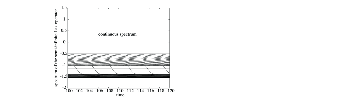
Figure 1.31: Evolution of $\sigma(L(t))$; driver: $x_{0}(t)=t+0.2(\sin\gamma t+0.5\cos 2\gamma t),\gamma=1.8,\gamma_{1}>\gamma>\gamma_{2}$

We see that $\sigma(L(t))$ converges to two bands separated by a gap, and a single phase wave emerges. For $\gamma_{2}>\gamma>\gamma_{3}$, we see from Figure 1.32

Figure 1.32: Evolution of $\sigma(L(t))$; driver: $x_{0}(t)=t+0.2(\sin\gamma t+0.5\cos 2\gamma t),\gamma=1.1,\gamma_{2}>\gamma>\gamma_{3}$

that $\sigma(L(t))$ converges to three bands separated by two gaps, and a two phase wave emerges, etc.
Remarks on the eigenvalues in the gap.

• The eigenvalues which can be observed in the gaps of the spectrum of the semi-infinite Lax operator $L(t)$ (compare with Figures 1.31 and 1.32) are of two different types. They are either constant in time or they move down from the lower edge of one band to the upper edge of the next band. Eigenvalues of the second kind can be understood from the corresponding $g$-gap solution They are connected to the zeros of a theta function, which is used in the construction of the $g$-gap solution (see Chapter 5). Eigenvalues which are constant in time can be interpreted as follows. Numerical computations show that they correspond to eigenvectors which are moving out as $t\rightarrow\infty$. Hence the eigenvalues do not survive in the spectrum of the limiting operator $L$, which corresponds to a lattice where all particles perform time periodic motion. In other words, from the spectral theoretic point of view, this is an example of the general phenomenon that under strong convergence of operators the spectrum is not necessarily conserved.

• Figures 1.31 and 1.32 give the impression that the eigenvalue branches which come down cross the eigenvalues, that remain constant in time. This, of course, is not possible as the symmetric, tridiagonal operator $L$ cannot have double eigenvalues. Instead, a close look demonstrates, that a billard ball collision is taking place as shown in Figure 1.33. It is possible to analyze the interaction of $\lambda_{k}$ and $\lambda_{k+1}$ in detail by using equation (2.5) of Chapter 2 for $j=k$ and $j=k+1$, together with the asymptotic assumption that $|\lambda_{k}-\lambda_{k+1}|$ is much smaller than the distance between any two other eigenvalues, but we do not present the details.

Figure 1.33: Close look at a “collision” of two eigenvalues

For $\lambda<\inf\sigma_{ess}(L(0))$, an interesting quantity to compute is

(1.34) $$J(\lambda)=\mathop{\lim}\limits_{t\rightarrow\infty}\,\,\,\frac{\sharp\,\,\{{\rm eigenvalues}\,\,{\rm of}\,\,L(t)\,\,{\rm that}\,\,{\rm are}\,\,<\lambda\}}{t}.$$

Clearly $J(\lambda)$ represents the asymptotic flux of eigenvalues of $L(t)$ across the value $\lambda$. In Chapter 2 we will extend the definition of $J$ to all values of $\lambda$.

It is observed numerically that $J(\lambda)$ indeed exists and for $\gamma_{2}>\gamma>\gamma_{3}$, say, we find that $J(\lambda)$ looks as displayed in Figure 1.35

Figure 1.35: Numerically observed $J(\lambda)$ in the case $\gamma_{2}>\gamma>\gamma_{3},\gamma=1.1$

Thus $J(\lambda)$ is constant in the gaps and indeed we observe more generally that

(1.36) $$J(\lambda)=\frac{j\gamma}{2\pi}\quad{\rm for}\quad\lambda\,\,{\rm in}\,\,{\rm the}\,\,j^{\rm th}\,\,{\rm gap}.$$

This is a very intriguing fact, reminiscent of the Johnson-Moser gap labelling theorem [JM] in the spectral theory of one-dimensional Schrödinger operators with almost periodic potentials (see also the analogous gap labelling theorem for Jacobi matrices [B], [S]).

Finally we are at the stage where we can describe our analytical results, whose goal is to explain the above numerical experiments. In the Toda case with constant driving, it was possible, using the exact formulae of inverse scattering, to show that the solution of the initial value problem converges as $t\rightarrow\infty$ to the binary motion if $a>1$, and to a quiescent lattice if $a<1$. In the present case, where we no longer have these formulae, our goals are more modest and we restrict our attention to a description of the observed attractor. Our results are the following:

I. Strongly nonlinear case.

Here we consider (1.18) in the case of the Toda lattice without any smallness restriction on the size of the oscillatory component $h$ of the driver $x_{0}$. The main result is Theorem 2.38 below in which we show how to compute the normalized density of state $J(\lambda)$ through the solution of a linear integral equation, once the number and endpoints of the bands in $\sigma(L(\infty))$ are known. This linear equation, in turn, can be solved explicitly via an associated Riemann-Hilbert problem.

At this stage it is not clear how to relate the number and endpoints of the bands to the parameters of the problem $a,\gamma,h$. To test Theorem 2.38 in any given situation, one reads off the discrete information given by the number and endpoints of the bands from the numerical experiment, and then compares the solution of the integral equation with the normalized density of states $J(\lambda)$ obtained directly from definition (1.33) using the numerically computed eigenvalues of $L(t)$ at large times. The numerical and analytical solutions for $J(\lambda)$ agree to very high order: see Appendix C (Figures C.12, C.13) for further details.

The proof of this result proceeds by deriving an equation of motion (see (2.5)) for the eigenvalues of a truncated version of $L(t)$ of size $N\gg t$ as $t\rightarrow\infty$. The continuum limit of the time average of these equations, leads to the linear integral equation (2.28) for $J(\lambda)$.

II. Weakly nonlinear case.

Here we consider general $F$, but the periodic component $h$ is now required to be suitably small. From the numerical experiments we see that if $h=0(\varepsilon)$, then as $t\rightarrow\infty,\,\,x_{n}(t)$ converges to an asymptotic state which is a $\frac{2\pi}{\gamma}$-time periodic solution $x_{{\rm asymp},\,n}(t)$ with $x_{{\rm asymp},\,n}(t)=cn+0(\varepsilon)$ for some lattice spacing $c$. The goal here is prove that such time periodic asymptotic states $x_{{\rm asymp},\,n}(t)$ indeed exist for $\varepsilon$ small. We proceed by linearizing around the particular solution $x_{{\rm asymp},\,n}(t)=cn,\,\,n\geq 0$, of the equations $\ddot{x}_{n}=F(x_{n-1}-x_{n})-F(x_{n}-x_{n+1}),\,\,n\geq 1$, and use various tools from implicit function theory.

Our first result (Theorem 3.38) is a nonlinear version of the classical linear method of separation of variables. For example, in solving the heat equation $u_{t}=u_{xx}$ on a half-line $x\geq 0$ with boundary conditions at $x=0$, one proceeds by expressing the solution as a combination

$$\int\,\,a_{+}(z)\,\,e^{-(tz^{2}+ixz)}dz+\int\,\,a_{-}(z)\,\,e^{-(tz^{2}-ixz)}$$

of elementary solutions $e^{-(tz^{2}\pm ixz)}$ of the heat equation on the full line, and then choosing the parameters $a_{+},a_{-}$ to satisfy the boundary condition at $x=0$. In the nonlinear case (Theorem 3.38) we show that provided a sufficiently large parameter family of travelling wave solutions of the doubly infinite lattice

(1.37) $$\ddot{x}_{n}=F(x_{n-1}-x_{n})-F(x_{n}-x_{n+1}),\,\,\,-\infty<n<\infty,$$

exist, then (modulo technicalities, see Chapter 3) the parameters can always be chosen to produce the desired asymptotic states $x_{{\rm asymp},\,n}(t)$ of the driven semi-infinite problem.

Thus the problem of the existence of the observed asymptotic states, reduces to the problem of constructing sufficiently large parameter families of travelling waves of the full lattice equation (1.37). As we will see in Chapter 3, for $\gamma_{k}>\gamma>\gamma_{k+1}\,\,k\geq 1$, we will need $2k$-parameter families of $k$-phase travelling waves of type (1.22) on the full lattice in order to construct the solution of the driven lattice observed as $t\rightarrow\infty$ in the numerical experiments. If $\gamma>\gamma_{1}$ (see Section 3.4) the requirement of travelling wave solutions of (1.37) trivializes, and Theorem 3.38 guarantees the existence of the desired asymptotic states $x_{{\rm asymp},\,n}(t)$ of the driven lattice for sufficiently small $h$ and general real analytic $F$ which are monotone in the region of interest, and this explains Figure C.6.

The next result (Theorem 4.24) concerns general $F$ in the case that $\gamma_{1}>\gamma>\gamma_{2}$. Here we show that a 2-parameter family of one-phase travelling wave solutions of (1.37) always exist for general $F$. Together with Theorem 3.38, this implies that for $\gamma_{1}>\gamma>\gamma_{2}$ the desired states $x_{{\rm asymp},\,n}(t)$ of the driven lattice exist, and this explains Figure C.7. This 2-parameter family is constructed by deriving an equation for the Fourier coefficients of the travelling wave solution, which can be solved by a Lyapunov-Schmidt decomposition. The infinite dimensional part does not pose any problems (see Lemma 4.19) and the degenerate finite dimensional equations can be solved by using certain symmetries of the equation (see Lemma 4.20).

If we try a similar construction for $m_{0}$-phase waves, $m_{0}>1$, then we encounter in the infinite dimensional part of the Lyapunov-Schmidt decomposition, a small divisor problem related to the small divisor problem occurring in [CW], where periodic solutions of the nonlinear wave equation are constructed, and which we hope to solve in the near future. In the special case of Toda, however, the family of travelling waves can be constructed explicitly. Indeed in our third, and final, result (Theorem 5.13) we use the integrability of the doubly infinite Toda lattice and show how the well-known class of $g$-gap solutions contains a sufficiently large family of travelling waves to apply to Theorem 3.38 and so construct the desired asymptotics states $x_{{\rm asymp},\,n}(t)$ of the driven lattice for any $\gamma\in{R}_{+}\backslash\{\gamma_{1},\gamma_{2},\cdots\}$.


Finally we want to pose four open problems, which are connected to our investigations, some of which were mentioned above.

• The “critical shock” phenomena.

  As discussed in the very beginning of the introduction, Holian and Straub have numerically discovered a critical shock strength $a_{{\rm crit}}(F)$ in the case of constant driving velocity $x_{0}(t)=2at$. For $a<a_{{\rm crit}}(F)$ the lattice comes to rest behind the shock front as $t\rightarrow\infty$, whereas for $a>a_{{\rm crit}}(F)$ the particles of the lattice will execute binary oscillations as $t\rightarrow\infty$. So far this result has been analytically explained in the case of the Toda lattice ($F(x)=e^{x}$) (cf [HFM], [VDO]) and can be seen to be absent for linear force functions by explicit calculation.

  The question is to find general conditions on the force $F$ for which one can prove the existence of a critical shock strength.

• Existence of multi-phase travelling waves.

  Let $F,c$ satisfy the general assumptions (cf Section 3.2.2) and let $\gamma\in{{R}}$ satisfy $\frac{2}{k}\sqrt{F^{\prime}(-c)}>\gamma>\frac{2}{k+1}\sqrt{F^{\prime}(-c)}$ for some $k\in{{N}}$.

  Does there exist a smooth $2k$-real parameter family of solutions

  (1.38) $$x_{n}(q)(t)=cn+\chi_{k}(q)(n\beta_{1}(q)+\gamma t,\ldots,n\beta_{k}(q)+k\gamma t),$$

  for $q\in{{R}}^{2k},q$ small, of the equation

  (1.39) $$\ddot{x}_{n}(t)=F(x_{n-1}-x_{n})-F(x_{n}-x_{n+1}),n\in{{Z}},$$

  where $\chi_{k}(q)$ is for each $q$ a function periodic in its $k$ arguments, $\chi_{k}(0)=0$ and $D_{q}\chi_{k}(0)$ has maximal rank $2k$? Note that these solutions exist in the case of the Toda lattice and are given by (5.10). For general force functions the work of Craig and Wayne ([CW]) indicates that it might be necessary to aim for a slightly weaker result, namely, that the smooth family of functions $x_{n}(q)(t)$ of the form (1.38) are solutions of (1.39) only for a Cantor set in the parameter space $q\in{{R}}^{2k}$, which has almost full measure.

• The case $a>a_{{\rm crit}}$.

  In the paper we always assume that the driver is of the form $x_{0}(t)=2at+h(\gamma t)$ with $a<a_{{\rm crit}}$. In the case of the Toda lattice we have also conducted some experiments for $a>a_{{\rm crit}}(Toda)=1$. We have made the following observation: for $h$ small, the limiting operator $L(t),t\rightarrow\infty$ seems to have infinitly many gaps and again we obtain a version of gap labelling. In fact, for all the gaps we have observed that one can write the numerically determined integrated spectral density $J(\lambda)$ (cf 1.34) in the form

  (1.40) $$J(\lambda)=\frac{j\gamma+k\omega}{2\pi},\quad j,k\in{{Z}},\quad\lambda\mbox{ lies in a gap, }$$

  where $\gamma$ denotes the frequency of the driver and $\omega$ is given by the frequency of the time-asymptotic oscillations, which are observed in the case that the driver has constant speed $x_{0}(t)=2at,a>1$.

  Corresponding to our results in Chapter 5, we ask whether it is possible to construct solutions of the driven semi-infinite Toda lattice with driver $x_{0}(t)=2at+h(\gamma t)$, such that the spectrum of the corresponding Lax-operator has infinitely many gaps and bands.

• Connection to the initial value problem.

  All of our results were motivated by the numerically observed long-time behavior of a certain initial value problem (with shock initial data). However, so far we are not able to prove from first principles, that the solution of the initial value problem actually converges as $t\rightarrow\infty$ to one of the asymptotic states described in Chapters 2-5. This basic problem remains open and, alas, seems far from a resolution.

Acknowledgments.

The work of the first author was supported in part by NSF Grant No. DMS–9203771. The work of the second author was supported in part by an Alfred P. Sloan Dissertation Fellowship. The work of the third author was supported by ARO Grant No. DAAH04-93-G-0011 and by NSF Grant No. DMS-9103386-002. The authors would also like to acknowledge the support of MSRI and the Courant Institute in preparing this videotext. Finally, the authors are happy to acknowledge useful conversations with many of their colleagues, and in particular, with Gene Wayne and Walter Craig. Also we would like to thank Fritz Gesztesy for making available his very useful notes ([G1], [G2]) on the application of the theory of Riemann surfaces to integrable systems.

Chapter 2 An asymptotic calculation in the strongly nonlinear case

2.1 The evolution equations

We recall from the Introduction the Flaschka variables (see (1.12))

(2.1) $$a_{n}=-\frac{\dot{x}_{n}}{2},\quad b_{n}=\frac{1}{2}e^{(x_{n}-x_{n+1})/2},\quad n=0,1,2,\dots,$$

$a_{n}\rightarrow a,\quad b_{n}\rightarrow\frac{1}{2}\quad\mbox{ as }~{}n\rightarrow+\infty,$

and we note that the function $a_{0}(t)$ is the given time-periodic forcing function. For the semi-infinite Toda chain with $F(x)=e^{x}$, equation (1.1) reduces to the perturbed Lax pair equation

(2.2) $$\frac{dL}{dt}+LB-BL=-\rho(t)P,$$

where $L$ is the tridiagonal operator (cf (1.27))

$$L=\left(\begin{array}[]{ccccc}a_{1}&b_{1}&&&0\\ b_{1}&a_{2}&b_{2}&\\ &b_{2}&a_{3}&b_{3}\\ 0&&\ddots&\ddots&\ddots\end{array}\right).$$

$B$ is the antisymmetric tridiagonal operator given by

$$B=\left(\begin{array}[]{ccccc}0&b_{1}&&&0\\ -b_{1}&0&b_{2}\\ &-b_{2}&0&b_{3}\\ 0&&\ddots&\ddots&\ddots\end{array}\right).$$

P is the rank-one matrix given by:

$$P_{ij}=\left\{\begin{array}[]{lll}1,&\mbox{ if }\qquad i=j=1\\ 0,&\mbox{ otherwise }\end{array}\right.$$

and $\rho(t)$ is the function:

(2.3) $$\rho(t)=2b_{0}^{2}(t)=2b_{1}^{2}(t)-\dot{a}_{1}(t),\quad\cdot=\frac{d}{dt}\;.$$

The matrices $L$ and $B$ are semi-infinite. We truncate the chain at some particle of very large index $N$, and work with the truncated finite matrices $L_{N}$ and $B_{N}$. The disturbance in the chain caused by the truncation, travels essentially with finite velocity. Only exponentially small effects display infinite speed. The bulk of the chain essentially does not feel the truncation until a time $t=O(N)$. Thus, we expect that the finite system is a good approximation to the full semi-infinite system in the space-time region $1<<t<<N$ and $n<<N$. In what follows, when we take the limit as $t\rightarrow\infty$, we always understand $t\to\infty,~{}N\to\infty,~{}\frac{t}{N}\to 0$.

We remark that on $\sigma_{ess}(L(t))=\sigma_{ess}(L(0))$, by standard spectral methods, the matrix $L_{N}(t)$ has a set of discrete eigenvalues tightly packed at densities of order $O(N)$. On the other hand, we expect that the discrete spectrum of $L(t)$, which emerges from $\sigma_{ess}(L(0))$ as described in the introduction, is well approximated by the eigenvalues of  $L_{N}(t)$ which lie outside $\sigma_{ess}(L(0))$. This is because the associated eigenvectors are typically exponentially decreasing in $n$ and hence do not feel the truncation at $N$.

A word of explanation: Typically an eigenvalue of $L_{N}(t)$ starts off as an eigenvalue of $L_{N}(0)$ lying in $\sigma_{ess}(L(0))$. As $t$ increases, the eigenvalue moves with velocity $O(\frac{1}{N})$ until it emerges from $\sigma_{ess}(L(0))$. It is only after this point that the motion of the eigenvalue becomes relevant to the evolution of the discrete spectrum of $L(t)$.

Our strategy is to derive evolution equations for

1. (a) the eigenvalues $\lambda_{j}^{N}$ of the truncated matrix $L_{N}$,

   (b) the first entry $f_{j}$ of the $j^{th}$ eigenvector of $L_{N}~{}(j=1,\dots,N)$ when it is normalized to have Euclidean length equal to one.

It is well known that the set $\{\lambda_{j},f_{j}\}^{N}_{j=1}$ determines the tridiagonal matrix $L_{N}$.

Theorem 2.4

The evolution of the $\lambda_{j}$’s and $f_{j}$’s is given by:

(2.5) $$\left\{\begin{array}[]{ll}\frac{1}{2}\frac{d}{dt}\ln(-\dot{\lambda}_{j})=\lambda_{j}-a_{0}(t)+\sum^{N}_{\stackrel{{\scriptstyle i=1}}{{\scriptscriptstyle{i\neq j}}}}\frac{\dot{\lambda}_{i}}{\lambda_{j}-\lambda_{i}},\quad~{}j=1,\dots,N\;,\\ f^{2}_{j}=\frac{-\dot{\lambda}_{j}}{\rho}\;,\end{array}\right.$$

where $\rho=2b_{0}^{2}(t)=-\sum^{N}_{i=1}\dot{\lambda}_{i}$. The initial values $\lambda_{i}(0)$ are the eigenvalues of $L_{N}$ at $t=0$ while the initial values $\dot{\lambda}_{i}(0)$ are given by

(2.6) $$\dot{\lambda}_{i}(0)=-2b_{0}^{2}(0)f_{i}^{2}(0).$$

Proof : Let $\Lambda$ be the diagonal matrix of the eigenvalues $\lambda_{j}$ of $L_{N}$ and let $\Psi$ be the orthogonal matrix whose $j^{th}$ column is the normalized eigenvector of $L_{N}$ corresponding to the eigenvalue $\lambda_{j}$. We have:

(2.7) $$L_{N}\Psi=\Psi\Lambda,$$

and we define the matrix $\Phi$ by:

(2.8) $$\Phi=\dot{\Psi}-B_{N}\Psi.$$

Utilizing equations (2.7) and (2.8) and (2.2), we easily calculate:

(2.9) $$L_{N}\Phi-\Phi\Lambda=\Psi\dot{\Lambda}+\rho P\Psi.$$

We now define the matrix $A=(a_{ij})$ by

(2.10) $$A=\Psi^{-1}\Phi=\Psi^{T}\Phi.$$

We calculate

$$A+A^{T} = \Psi^{T}\Phi+\Phi^{T}\Psi$$

$$= \Psi^{T}(\dot{\Psi}-B_{N}\Psi)+(\dot{\Psi}^{T}-\Psi^{T}B_{N}^{T})\Psi$$

$$= \Psi^{T}\dot{\Psi}+\dot{\Psi}^{T}\Psi=\frac{d}{dt}(\Psi^{T}\Psi)=0.$$

Thus

(2.11) $$A+A^{T}=0;$$

i.e. $A$ is antisymmetric. Using (2.9) we obtain

(2.12) $$L_{N}\Phi-\Phi\Lambda=L_{N}\Psi A-\Psi A\Lambda=\Psi(\Lambda A-A\Lambda).$$

Comparing (2.9) with (2.12) we obtain easily:

(2.13) $$\dot{\Lambda}=[\Lambda,A]-\rho\Psi^{T}P\Psi.$$

Let $f^{T}=(f_{1},f_{2},\dots,f_{N})$ be the first row of $\Psi$. Then $\Psi^{T}P\Psi=ff^{T}$. We insert this relation in (2.13),

(2.14) $$\dot{\Lambda}=[\Lambda,A]-\rho ff^{T}.$$

Equating the diagonal elements on both sides we obtain:

(2.15) $$\dot{\lambda}_{j}=-\rho f^{2}_{j},\qquad\sum^{N}_{j=1}\dot{\lambda}_{j}=-\rho.$$

This proves the second relation in Theorem 2.4. Furthermore we note that the first components $f_{j}$ of the eigenvectors of the tridiagonal matrix $L_{N}$ do not vanish and we conclude by (2.15) that $-\dot{\lambda}_{j}>0$. Hence the first relation in Theorem 2.4 is well defined.

Off the diagonal in (2.14) we have $\lambda_{i}a_{ij}-a_{ij}\lambda_{j}=\rho f_{i}f_{j}$. On the other hand $a_{ii}=0$ by (2.11). Thus

(2.16) $$\begin{array}[]{l}\left\{\begin{array}[]{lll}a_{ij}&=&\frac{\rho f_{i}f_{j}}{\lambda_{i}-\lambda_{j}},\quad\mbox{ when }\quad i\neq j,\\ a_{ii}&=&0.\end{array}\right.\end{array}$$

We now calculate the evolution of $f_{j}$. By (2.8):

$$\dot{\Psi}=\Phi+B_{N}\Psi=\Psi A+B_{N}\Psi.$$

Specializing to the first row we obtain $\dot{f}^{T}=f^{T}A+B_{R_{1}}\Psi$, where $B_{R_{1}}$ is the first row of $B_{N}$. This implies

$$\dot{f}^{T} = f^{T}A+(L_{N}-a_{1}I)_{R_{1}}\Psi=f^{T}A+(L\Psi)_{R_{1}}-a_{1}f^{T}$$

$$= f^{T}A+(\Psi\Lambda)_{R_{1}}-a_{1}f^{T}=f^{T}A+f^{T}\Lambda-f^{T}a_{1},$$

or, taking transposes

(2.17) $$\dot{f}=(\Lambda-a_{1}I-A)f.$$

But, by (2.16),

(2.18) $$A=\rho FDF,$$

where $F$ is the invertible diagonal matrix with entries $f_{1},\dots,f_{N}$ and $D$ is the matrix $\left(\frac{1}{\lambda_{i}-\lambda_{j}}\right)$ with zero entries on the diagonal. Thus $\dot{f}=(\Lambda-a_{1}I-\rho FDF)f$, and hence

(2.19) $$F^{-1}\dot{f}=F^{-1}\Lambda f-a_{1}F^{-1}f-\rho DFf.$$

Now note that

1. $\rho Ff=\rho\left(\begin{array}[]{cc}f_{1}^{2}\\ f_{2}^{2}\\ \vdots\end{array}\right)=-\left(\begin{array}[]{cc}\dot{\lambda}_{1}\\ \dot{\lambda}_{2}\\ \vdots\end{array}\right)$ by (2.15),

2. $F^{-1}f=\left(\begin{array}[]{cc}1\\ 1\\ \vdots\end{array}\right)$,  $F^{-1}\Lambda=\Lambda F^{-1}$.

Substituting in (2.19) we obtain

(2.20) $$\frac{\dot{f}_{j}}{f_{j}}=\lambda_{j}-a_{1}+\sum\limits^{N}_{\stackrel{{\scriptstyle i=1}}{{\scriptscriptstyle{i\neq j}}}}\frac{\dot{\lambda}_{i}}{\lambda_{j}-\lambda_{i}}.$$

The evolution of the $\lambda_{i}$’s in (2.5) is finally obtained by eliminating $f_{j}$ between (2.20) and (2.15) and using the expression for $\rho$ given in (2.3).

$\Diamond$

2.2 The continuum limit of eigenvalue dynamics

The results of the numerical experiments described in the Introduction, (cf Figures 1.29-(1.32 lead us to consider the flux of eigenvalues of the matrix $L_{N}$ across a value $\lambda$. Noting that the eigenvalues of $L_{N}$ move toward lower values $(\dot{\lambda}_{i}=-\rho f^{2}_{i}<0)$, we define the eigenvalue flux at $\lambda$ averaged over a time interval $(t,t+T)$ by

(2.21) $$J_{t,T}(\lambda)=\frac{1}{T}~{}\mbox{ card }~{}\{{i}:\lambda_{i}(t+T)<\lambda<\lambda_{i}(t),~{}~{}i=1,2\ldots N\}.$$

We pose the following ansatz.

Ansatz 2.22

There exists a continuous, almost everywhere continuously differentiable function $J(\lambda)$ such that

(2.23) $$J_{t,T}(\lambda)\to J(\lambda),\quad\mbox{ when }\quad T,t,N\to\infty\quad\mbox{ subject to }\quad T<t\ll N.$$

When $\lambda<inf~{}\sigma_{ess}(L)$, it is clearly true that

(2.24) $$J(\lambda)=\lim\limits_{t\to\infty}\displaystyle\frac{\mbox{ \# eigenvalues of }~{}L(t)~{}\mbox{ that are smaller than }~{}\lambda}{t}~{},$$

as defined in the Introduction. The net gain in eigenvalues of $L_{N}$ of an interval $({\lambda},\hat{\lambda})$ over a long time $T$ is given asymptotically by $[J(\hat{\lambda})-J(\lambda)]T.$ Dividing by $(\hat{\lambda}-\lambda)T$ and letting $\hat{\lambda}\to\lambda$ we obtain that the asymptotic rate of increase in eigenvalue concentration at $\lambda$ is given by $\frac{dJ}{d\lambda}=J^{\prime}(\lambda)$; thus, the difference in eigenvalue concentration at $\lambda$ between times $t$ and zero is asymptotically $tJ^{\prime}(\lambda)$. When $\lambda<inf~{}\sigma_{ess}(L)$, necessarily $J^{\prime}(\lambda)\geq 0$ since there is no original eigenvalue concentration at $\lambda$. On the other hand $J^{\prime}(\lambda)$ can take negative values when $\lambda\in\sigma_{ess}(L)$.

We will now use the function $J(\lambda)$ and some assumptions based on numerical observations to derive the continuum limit of the eigenvalue evolution equations (2.5). We begin by averaging the system (2.5) of equations $(j=1,\ldots N)$ over the time interval $(t,t+T)$ to obtain

(2.25) $$\frac{1}{2T}\ln\displaystyle\frac{\dot{\lambda}_{j}(t+T)}{\dot{\lambda}_{j}(t)}=$$

$$\frac{1}{T}\int^{t+T}_{t}\lambda_{j}(t^{\prime})dt^{\prime}-\displaystyle\frac{1}{T}\int^{t+T}_{t}a_{0}(t^{\prime})dt^{\prime}+\displaystyle\frac{1}{T}\sum\limits^{N}_{i=1\atop i\neq j}\int^{t+T}_{t}\displaystyle\frac{d\lambda_{i}(t^{\prime})}{\lambda_{j}(t^{\prime})-\lambda_{i}(t^{\prime})},\quad j=1,\ldots N.$$

Let $\lambda$ satisfy $J^{\prime}(\lambda)\neq 0$, and let $j=j(t)$ be such that in the asymptotic limit $1\ll T\ll t\ll N$ (note that we require $T\ll t$, not just $T<t$ as in (2.23)) the following is true,

(2.26) $$\lambda_{j(t)}(t^{\prime})\to\lambda\mbox{ for any }t^{\prime}\mbox{ that satisfies }t<t^{\prime}<t+T.$$

In practical terms, this means that we expect eigenvalues $\lambda_{j}$ to stay close to the value $\lambda$ throughout the time interval $[t,t+T]$. This fact is clearly borne out in the results of numerical experiments as long as $J^{\prime}(\lambda)\neq 0$.

We make two more simplifying assumptions when $J^{\prime}(\lambda)\neq 0$ that are again justified by numerical experiments:

• 1. The left hand side of (2.25) is negligible.

  2. The “singular contribution” in the sum of the right hand side corresponding to indices $i$ that are close to $j$ is also negligible. In practical terms we interpret this to mean that the limiting integral kernel is the Hilbert transform.

Under these conditions we can take the limit $1\ll T\ll t\ll N$ in (2.25)-(2.26).

Theorem 2.27

(Continuum Limit of (2.25)-(2.26)). Under Ansatz (2.22) and under the further assumption described above we have:

(2.28) $$J^{\prime}(\lambda)\neq 0\Rightarrow\lambda-<a_{0}>-\displaystyle\int\limits^{\infty}_{-\infty}\!\!\!\!\!\!\!\!=\frac{J(\mu)}{\lambda-\mu}d\mu=0,$$

where $<a_{0}>$ is the mean value of the periodic driver $a_{0}(t)$, and as usual the double bars on the integral indicate that the principal value is taken.

Proof : By the assumptions, and by (2.26) the only thing to be shown is that the sum in (2.25) tends to the integral in (2.28). If we partition the eigenvalue axis into a set of infinitesimal intervals and if $(\mu-d\mu,\mu)$ is such an interval then the contribution $\displaystyle\frac{1}{T}\left(\frac{-d\mu}{\lambda-\mu}\right)$ should arise in as many terms of the sum in (2.26) as there are eigenvalues that cross the value $\mu$ during the time interval $(t,t+T)$. This number is asymptotically $TJ(\mu)$. The sum in (2.26) therefore tends to $-\displaystyle\int\limits^{\infty}_{-\infty}\!\!\!\!\!\!\!\!=\frac{J(\mu)d\mu}{\lambda-\mu}$.

$\Diamond$

2.3 The asymptotic spectral density of $L_{N}$

We now consider the problem of determining $J(\lambda)$. Our solution is partial in the sense that we can calculate the function $J(\lambda)$ if we are given the set $\{\lambda:J^{\prime}(\lambda)\neq 0\}$. Numerical calculations (see Figures 1.31, 1.32, 1.35) show that this set is a finite union of intervals. Thus, we are assuming knowledge of a finite set of numbers that are in principle determined by the fluctuating part of the periodic driver $a_{0}(t)$. Determining these numbers is, unfortunately, the part of the problem that we have not yet been able to solve.

We proceed to give some basic definitions.

Definition 2.29

Let the points $p_{0}<q_{1}<p_{1}<q_{2}<p_{2}<\ldots<p_{g}<q_{g+1}$ be given. These are $2g+2$ points in all. We define the set of bands $B$, where we have $J^{\prime}(\lambda)\neq 0$,

(2.30) $$B=[p_{0},q_{1}]\cup[p_{1},q_{2}]\cup\cdots\cup[p_{g},q_{g+1}],$$

and the set of gaps $G$, where $J^{\prime}(\lambda)=0$, by

(2.31) $$G_{k}=(q_{k},p_{k}),~{}k=1,2,\ldots g;\qquad G=\cup^{g}_{k=1}G_{k}$$

(cf Figure 2.36 below). We then define the hyperelliptic curve

(2.32) $$R(\lambda)=\{\Pi^{g}_{k=0}(\lambda-p_{k})(\lambda-q_{k+1})\}^{1/2}$$

with branch cuts along the set B and sign determination such that $R(\lambda)>0$ when $\lambda\to+~{}\infty$. Finally, we define the polynomial

(2.33) $$P(\lambda)=\displaystyle\sum\limits^{g+1}_{i=1}(\lambda-\sigma_{i})\quad,\sigma_{i}\in{\bf R},$$

where the $\sigma_{i}\mbox{'s},~{}i=1,\ldots g+1$, are uniquely determined by the $g+1$ relations.

(2.34) $$\int\limits_{G_{k}}\displaystyle\frac{P(\lambda)}{R(\lambda)}d{\lambda}=0\quad,k=1,2,\ldots g.$$

(2.35) $$\int\limits_{B}\displaystyle\frac{P(\lambda)}{R(\lambda)}d{\lambda}=0.$$

Figure 2.36: The band – gap structure of the spectrum

We observe that the integrals in (2.34) and (2.35) can be easily understood as contour integrals on the Riemann surface associated with $R$. The contour in (2.35) can be replaced by a circle of (large) radius. We then obtain $\frac{P(\lambda)}{R(\lambda)}=1+O(\frac{1}{\lambda^{2}})\quad\mbox{ as }\quad\lambda\to\infty$, which implies through an easy asymptotic calculation that

(2.37) $$2\displaystyle\sum\limits^{g+1}_{i=1}\sigma_{i}=\displaystyle\sum\limits^{g}_{i=0}(p_{i}+q_{i+1}).$$

Theorem 2.38

Let $J(\lambda)$ be a continuous function supported on the set $B\cup G$, differentiable at all points, except possibly the boundary points of $B$, satisfying

(2.39) $$\lambda-<a_{0}>-\displaystyle\int\limits^{\infty}_{-\infty}\!\!\!\!\!\!\!\!=\displaystyle\frac{J(\mu)}{\lambda-\mu}d\mu=0\qquad\lambda\in B,$$

(2.40) $$J(\lambda)=c_{k}=\mbox{ const., }\qquad\lambda\in G_{k},~{}k=1\ldots,g,$$

(2.41) $$J(\lambda)=0\qquad\lambda\not\in B\cup G,$$

where $<a_{0}>$ is a constant. Then $J(\lambda)+iHJ(\lambda)$ is the limiting value as $z\to\lambda+i0$, of the analytic function

(2.42) $$f(z)=\frac{-i}{\pi}\displaystyle\int\limits^{\infty}_{z}1-\displaystyle\frac{P(z^{\prime})}{R(z^{\prime})}dz^{\prime},\quad{\bf Im}~{}z\neq 0.$$

Precisely:

(2.43) $$J(\lambda)=\displaystyle\frac{1}{\pi}{\bf Im}\displaystyle\int\limits^{\infty}_{\lambda}\displaystyle\left(1-\frac{P(\mu)}{R(\mu)}\right)d\mu,$$

(2.44) $$HJ(\lambda)=\frac{1}{\pi}\displaystyle\int\limits^{\infty}_{-\infty}\displaystyle\frac{J(\mu)}{\lambda-\mu}d\mu=-\displaystyle\frac{1}{\pi}{\bf Re}\displaystyle\int\limits^{\infty}_{\lambda}\left(1-\displaystyle\frac{P(\mu)}{R(\mu)}\right)d\mu.$$

The endpoints of $B$ satisfy the compatibility condition

(2.45) $$q_{g+1}+\displaystyle\int\limits^{\infty}_{q_{g+1}}\displaystyle\left(1-\displaystyle\frac{P(\lambda)}{R(\lambda)}d\lambda\right)=<a_{0}>.$$

Remark 2.46

on condition (2.40).
In the above Theorem 2.38 we have not specified the value $c_{k}$ which the function $J(\lambda)$ obtains in the $k$-th gap. In fact, $c_{k}$ will be determined by all the other conditions of Theorem 2.38. However, as remarked in the Introduction (1.36), one observes in numerical experiments that $c_{k}$ should equal $k\gamma/2\pi$. Figures C.12 and C.13 in Appendix C demonstrate that the solution $J(\lambda)$ of the integral equation (2.39) – (2.41) indeed satisfies this additional relation.

Proof : The differentiability properties of $J(\lambda)$ in the interior of $B$ as well as its constancy on the $G_{k}$’s is immediately obvious as soon as one sees that $R$ is pure imaginary in the interior of $B$, and pure real elsewhere. The function $J(\lambda)$ is clearly continuous at the endpoints of each $G_{k}$ and at $q_{g+1}$. Also $J(p_{0})=0$ by (2.35) and consequently $J(\lambda)=0$ when $\lambda<p_{0}$. Condition (2.39) follows from (2.34), (2.44) and (2.45) in a straightforward way, using once again the pure real/pure imaginary structure of $R$.

The function $J(\lambda)$ constructed is unique. Indeed, if by $\delta(\lambda)$ we denote the difference of two solutions of (2.39)-(2.41), then $\delta(\lambda)$ satisfies the equations

(2.47) $$\left\{\begin{array}[]{rlll}H\delta(\lambda)&=0,&\mbox{ when }&\lambda\in B,\\ \delta(\lambda)&=c^{{}^{\prime}}_{k}=const.,&\mbox{ when }&\lambda\in G_{k},~{}n=1,\ldots g,\\ \delta(\lambda)&=0,&\mbox{ when }&\lambda\not\in B\cup G,\end{array}\right.$$

and its derivative $\delta^{\prime}(\lambda)$ satisfies

(2.48) $$\left\{\begin{array}[]{rlll}H\delta^{\prime}(\lambda)&=0,&\mbox{ when }&\lambda\in B,\\ \delta^{\prime}(\lambda)&=0,&\mbox{ when }&\lambda\not\in B.\end{array}\right.$$

By (2.48) and the third relation in (2.47) the derivative $\delta^{\prime}(\lambda)$ of $\delta(\lambda)$ is identically zero; since $\delta(\lambda)$ is compactly supported we also have $\delta(\lambda)=0.$

$\Diamond$

The above derivation of the equation for $J(\lambda)$ has been obtained under a variety of assumptions. A fully rigorous derivation still eludes us. At this stage however the justification lies in the comparison with experiments as described e.g. in Figures C.12 and C.13 of Appendix C.

Chapter 3 A boundary matching technique

3.1 Introduction

In this chapter we construct $\frac{2\pi}{\gamma}$ – time periodic solutions of

(3.1) $$\ddot{x}_{n}(t)=F(x_{n-1}(t)-x_{n}(t))-F(x_{n}(t)-x_{n+1}(t)),\quad n\geq 1,$$

with

(3.2) $$x_{0}(t):=\epsilon\sum_{m\in{{Z}}}b_{m}e^{i\gamma mt},\quad\sum_{m\in{{Z}}}|b_{m}|=1,$$

satisfying

(3.3) $$x_{n}(t)=cn+O(\epsilon).$$

Throughout this chapter we assume that $F$ is real analytic and monoton increasing on an open interval. We will construct solutions satisfying (3.1)-(3.3) for any $c\in{{R}}$, such that $-c$ lies in the interval. Not all values of $c$, however, can be observed as the spacing of an asymptotic state of the driven lattice, described by the initial boundary value problem 1.18. To see this we look at the Toda lattice. For $a<1$, in the case where $h=0$, the solution $x_{n}(t)$ converges as $t\rightarrow\infty$ to $x_{{\rm asymp},\,n}(t)=cn$, with spacing $c=-2\ln(1+a)$. Thus the values of the spacing $c$ that can be observed by driving the Toda lattice with constant velocity $2a$, lie between $-\ln 4$ and $0$. For $a>1$, as we know, the solution of the driven lattice does not converge to a quiescent state $x_{{\rm asymp},\,n}(t)=cn$ and, in particular, the values $c=-2\ln(1+a)$, for $a>1$ cannot be observed in this experiment.

Expand $x_{n}(t)$ in a Fourier series,

(3.4) $$x_{n}(t)=cn+\sum_{m\in{{Z}}}a(n,m)e^{i\gamma mt},\quad\mbox{ for }n\geq 0.$$

For $n=0$ we have $a(0,m)=\epsilon b_{m}$. Expanding $F$ in a power series at $-c$, we obtain

$$F(x_{n-1}-x_{n})-F(x_{n}-x_{n+1})$$

$$= F^{\prime}(-c)\sum_{m\in{{Z}}}[a(n-1,m)-2a(n,m)+a(n+1,m)]e^{i\gamma mt}+\mbox{ higher order terms }.$$

Equation (3.1) with (3.2) is equivalent to

(3.5) $$(L_{m}a(\cdot,m))(n)+W(a)(n,m)+a(0,m)\delta_{1,n}=0,\quad\mbox{ for all }m\in{{Z}},n\geq 1,$$

where for $m\in{{Z}}$ the linear operators $L_{m}$ acting on the $n$-variable are given by

(3.6) $$L_{m}=\left(\begin{array}[]{cccc}\delta_{m}&1&&0\\ 1&\delta_{m}&1&\\ &1&\delta_{m}&\ddots\\ 0&&\ddots&\ddots\\ \end{array}\right),\quad\delta_{m}:=-2+\frac{(m\gamma)^{2}}{F^{\prime}(-c)}.$$

$W(a)$ contains all terms of higher order and $\delta_{1,n}$ denotes the Kronecker symbol.

We note that for $\epsilon=0$ equation (3.5) is solved by $a=0$. However, we cannot apply the implicit function theorem to obtain solutions of equation (3.5) for $\epsilon\neq 0$, because the linearized operator,

(3.7) $$L=\bigoplus_{m\in{{Z}}}L_{m},$$

is not invertible. Indeed, the spectrum of the operator $L_{m}$ acting on $\ell_{2}$ sequences is given by $\sigma(L_{m})=[\delta_{m}-2,\delta_{m}+2]$. This implies that $0\in\sigma(L_{m})$ for all $m\in{{Z}}$ satisfying $0\leq\frac{(\gamma m)^{2}}{F^{\prime}(-c)}\leq 4$. Denote

(3.8) $$m_{0}:=\max\{m\in{{Z}}:0\leq\frac{(\gamma m)^{2}}{F^{\prime}(-c)}\leq 4\},$$

then the multiplicity of $0$ in the $\ell_{2}$ spectrum of $L$ is $2m_{0}+1$. However, due to the simple form of the operator $L_{m}$ we are able to “ invert ” the operator explicitly. In fact, consider the important case $0<\frac{(\gamma m)^{2}}{F^{\prime}(-c)}<4$. For a given vector $(y_{n})_{n\geq 1}$ and given $u_{1}$, the vector $(u_{n})_{n\geq 2}$ solves the equation

$$L_{m}u=y,$$

if and only if

$$u_{n} = \frac{1}{\sin\beta_{m}}\left[u_{1}\sin n\beta_{m}+\sum_{k=1}^{n-1}y_{k}\sin(n-k)\beta_{m}\right]$$

$$= \frac{1}{\sin\beta_{m}}\left[\sin n\beta_{m}\left(u_{1}+\sum_{k=1}^{n-1}y_{k}\cos k\beta_{m}\right)-\cos n\beta_{m}\sum_{k=1}^{n-1}y_{k}\sin k\beta_{m}\right],$$

(3.9) $$\beta_{m}:=-\mbox{ sgn }(m)\arccos\left(-\frac{\delta_{m}}{2}\right).$$

Note, that the value of $u_{n}$ is independent of the sign of $\beta_{m}$. We will justify the particular choice we have made in Section 3.3 (see (3.35)) below.

The following observation will prove to be useful. Suppose $(y_{n})_{n\geq 1}$ decays exponentially, i.e. there exists a $\sigma>0$, such that $\sup_{n\geq 1}\left|y_{n}e^{\sigma n}\right|<\infty$, then $\sup_{n\geq 1}\left|u_{n}e^{\sigma n}\right|<\infty$, provided the following two relations hold.

(3.10) $$u_{1}+\sum_{k=1}^{\infty}y_{k}\cos k\beta_{m}=0$$

and

(3.11) $$\sum_{k=1}^{\infty}y_{k}\sin k\beta_{m}=0.$$

Equation (3.10) can always be satisfied by an appropriate choice of $u_{1}$, whereas equation (3.11) is a condition on the sequence $(y_{n})_{n\geq 1}$. Therefore the operator $L_{m}$ acts 1-1 on spaces of exponentially decaying sequences and the range has codimension 1. Furthermore a simple calculation shows that the inverse operator acts on the range as a bounded operator with respect to the corresponding exponentially weighted supremum norms. Still we cannot apply a standard implicit function theorem to obtain solutions of equation (3.5). Nevertheless, proceeding formally, we transform equation (3.5) into a fixed-point equation.

(3.12) $$a(n,m)=-L_{m}^{-1}[W(a)(n,m)+\epsilon b_{m}\delta_{1,n}].$$

As $W$ is of higher order we can in principle apply a Banach fixed-point argument to obtain a solution of (3.12) as long as $L_{m}^{-1}$ is a bounded operator. We have seen above that this can be achieved, if condition (3.11) is satisfied, i.e.

(3.13) $$\epsilon b_{m}\sin\beta_{m}+\sum_{k=1}^{\infty}W(a)(k,m)\sin k\beta_{m}=0,\mbox{ for }0<\frac{(\gamma m)^{2}}{F^{\prime}(-c)}<4.$$

Equation (3.13) indicates that we will be able to solve equation (3.12) for sufficiently small $\epsilon$ in a space of sequences decaying exponentially in $n$, only if the Fourier coefficients of the driver $b_{m}$ take on a special value for those $m\in{{Z}}$ satisfying $0<\frac{(\gamma m)^{2}}{F^{\prime}(-c)}<4$.

This observation is consistent with the linear case where we conclude from formulae (1.23) – (1.25) that the solutions decay exponentially in $n$, only if $b_{m}=0$ for $0\leq\frac{(\gamma m)^{2}}{F^{\prime}(-c)}\leq 4$. The linear case also suggests that we should add multiphase waves in order to obtain solutions of equations (3.1),(3.2) for general driving functions. This leads to the following ansatz for $a(n,m)$:

(3.14) $$\hskip 14.22636pta(n,m)=u(n,m)+v(n,m)+(\epsilon b_{m}-u(0,m)-v(0,m)),\quad n\geq 0,m\in{{Z}},$$

where $u$ denotes the travelling wave part and $v$ corresponds to the exponentially decaying modes. Note that (3.14) implies $a(0,m)=\epsilon b_{m}$, for all $m\in{{Z}}$.

Definition 3.15

We will refer to the Fourier modes $m$ with $0\leq\frac{(\gamma m)^{2}}{F^{\prime}(-c)}\leq 4$, or equivalently $|m|\leq m_{0}$, as resonant Fourier modes. On the other hand we say that a frequency $\gamma\in{{R}}^{+}$ is resonant if $\frac{(\gamma m)^{2}}{F^{\prime}(-c)}=4$ for some $m\in{{Z}}$.

The present chapter is organized as follows. We begin Section 3.2 by deriving equations for the sequences of Fourier coefficients $u(n,m)$ and $v(n,m)$ (given by (3.4) and (3.14) above), which are sufficient to prove that the corresponding functions $x_{n}(t)$ solve (3.1), (3.2). These equations, which are given in Lemma 3.31 below, can be made rather explicit because of the assumption, that the force function $F$ can locally be expanded in a power series and therefore we will obtain good estimates on the higher order terms by carefully choosing the norm on the sequences of Fourier coefficients. In the notation of Lemma 3.31, these equations can be described as follows.

• is an equation for $u$, which is satisfied by the Fourier coefficients of solutions $x_{n}(t;u):=\sum_{m\in{{Z}}}u(n,m)e^{i\gamma mt}$ of the doubly infinite lattice.

• is an equation for $v$, depending on $u$, which guarantees that $u+v$ corresponds to a solution of the semi-infinite lattice.

• represents the boundary condition by requiring $\epsilon b_{m}-u(0,m)-v(0,m)=0$, for $m\neq 0$. The case $m=0$ is special; we do not have to require $\epsilon b_{0}-u(0,0)-v(0,0)=0$ for the reason that solutions of (3.1) are invariant under translations $x_{n}\rightarrow x_{n}+const$.

We then proceed in Section 3.3 to prove the basic result (Theorem 3.38) of this chapter. Assume $\gamma$ is non resonant (see Definition 3.15, then for (small) $\epsilon$ and for given (small) travelling wave solutions $u$ of the doubly infinite lattice, we can construct sequences $v$ satisfying equation (2) above and solving equation (3) for all non resonant Fourier modes $m$ (compare with Definition 3.15), i.e. for those $m\in{{Z}}$ satisfying $|m|>m_{0}$. Furthermore suppose that $u$ is given as a $C^{1}$ function of a parameter $q$. Then we will show that the resulting $v$ is a $C^{1}$ function of $q$ and $\epsilon$. Note that this statement is needed in order to ensure that the remaining equations of (3) (for resonant Fourier modes) can be solved by constructing a sufficiently large parameter family of travelling wave solutions $u(q)$, and then applying a standard implicit function theorem.

The proof of this basic result (Theorem 3.38) rests on a Banach fixed-point argument. The equation for $v$ takes the form

(3.16) $$(Lv)(n,m)+W(u,v)(n,m)+v(0,m)\delta_{1,n}=0,\mbox{ for }n\geq 1,m\in{{Z}}.$$

$L=\bigoplus_{m\in{\scriptsize{{Z}}}}L_{m}$ was defined in (3.6) and (3.7) and $W(u,v)$ denotes the higher order terms. We turn (3.16) formally into a fixed-point equation,

(3.17) $$v(\cdot,m)=-L_{m}^{-1}\left(W(u,v)(\cdot,m)+v(0,m)\delta_{1,\cdot}\right).$$

Denote

$$S_{\sigma}:=\left\{(y_{n})_{n\geq 1}:\sup_{n\geq 1}\left|y_{n}e^{\sigma n}\right|<\infty\right\}.$$

As indicated above we will be able to prove the following results on the invertibility of $L_{m}$ by explicit calculation (see proof of Theorem 3.38).

• For $0<|m|\leq m_{0}$ and $\sigma>0$, the linear operator $L_{m}$ maps $S_{\sigma}$ onto $\{y\in S_{\sigma}:\sum_{k\geq 1}y_{k}\sin(k\beta_{m})=0\}$. (The quantities $\beta_{m}$ were defined in (3.9). The inverse operator acting on the range is bounded with respect to the corresponding norms.

• There exist weights $\sigma>0$, such that the operators $L_{m}:S_{\sigma}\rightarrow S_{\sigma}$ are bijective and have a bounded inverse for all $|m|>m_{0}$.

• Again the case $m=0$ is somewhat special as the Green’s function of the operator $L_{0}$ grows linearly and we will have to use the special structure of $W(u,v)$ in order to define a bounded inverse. See the proof of Theorem 3.38 below for more details.

Although $u(n,m)$ does not decay in $n$, we will nevertheless see by explicit calculation that $W(u,v)$ decays exponentially in $n$. This makes it possible to prove the exitence of a solution of (3.17) by a Banach fixed-point argument. For $|m|>m_{0}$ we can choose $v(0,m)=\epsilon b_{m}-u(0,m)$ and hence satisfy the boundary condition as described in equation (3) above, whereas in the case $0<|m|\leq m_{0}$ the choice of $v(0,m)$ is determined by the condition that $W(u,v)(\cdot,m)+v(0,m)\delta_{1,\cdot}$ has to lie in the range of $L_{m}$. A small technical problem arises when proving the smooth dependence of $v$ on the parameters. It will turn out that the travelling wave solutions constructed in the subsequent chapters depend smoothly on $q$, but $\frac{\partial u}{\partial q}(n,m)$ grows linearly in $n$. Therefore $\frac{\partial u}{\partial q}$ does not lie in a space which is suitable for our calculations. We will verify the smooth dependence of $v$ on $q$ and $\epsilon$ explicitly by applying a Banach fixed-point argument to the partial derivatives in the appropriate spaces.

In Section 3.4 we show that the results of Sections 3.2 and 3.3 suffice to construct periodic solutions of the driven lattice in the case that $m_{0}=0$, which corresponds to high driving frequencies.

3.2 The equation for the Fourier coefficients

In this section we introduce norms, which are suitable for the sequences of Fourier coefficients, and prove some of their basic properties. Then the general assumptions on the force function $F$ and on the driver will be stated precisely. Using the assumptions on $F$ we derive estimates on the nonlinear terms which allow us to give conditions on the Fourier coefficients which are sufficient for proving that the correponding functions $x_{n}(t)$ given by (3.4) and (3.14) solve equations (3.1) and (3.2).

3.2.1 Sequence spaces

The choice for the norms on the sequences of Fourier coefficients $u(n,m)$ and $v(n,m)$ (compare with equation (3.14)) is motivated by the following observations. The nonlinear terms of the force function make it necessary to take convolutions with respect to the $m$-variable (see Section 3.2.3 below). Therefore we choose an $\ell_{1}$-norm for $m$. In fact we use a weighted $\ell_{1}$-norm in order to control the regularity of the solution. Furthermore the weight function has to satisfy some additional conditions to insure that the norm is still compatible with respect to convolution (see Definition 3.18 of admissible weight functions). For the $n$-variable a supremum norm with an exponential weight is chosen which is suitable for inverting the linearized operators $L_{m}$.

Definition 3.18

A map $w:{{Z}}\rightarrow{{R}}$ is said to be an admissible weight function, if

(3.19) $$w(m)\geq 1,\quad\mbox{ for all }m\in{{Z}},$$

and

(3.20) $$w(m)\leq w(m-n)w(n),\quad\mbox{ for all }m,n\in{{Z}}.$$

Definition 3.21

Let $w$ be an admissible weight function. We denote

$$\ell_{1,w}:=\left\{u:{{Z}}\rightarrow{{C}}\left|\sum_{m\in{{Z}}}w(m)|u(m)|<\infty\right.\right\},$$

with the corresponding norm

$$\|u\|_{\ell_{1,w}}:=\sum_{m\in{{Z}}}w(m)|u(m)|.$$

Note that $\ell_{1,w}$ is a Banach space which lies in $\ell_{1}$ by condition (3.19). The inequality (3.20) insures that the $\ell_{1,w}$-norm is submultiplicative with respect to convolution (see Proposition 3.23 below). It also implies that the weight function can not grow faster than exponentially. Indeed, it is easy to prove that $w(m)\leq w(0)\left(\max(w(1),w(-1))\right)^{|m|}$. We shall be interested in three types of weight functions which will all satisfy the conditions specified in Definition 3.18.

• $\forall m\in{{Z}}:w(m):=1$ .

• $\forall m\in{{Z}}:w(m):=(1+|m|)^{\beta}$, for $\beta\geq 0$ .

• $\forall m\in{{Z}}:w(m):=e^{\beta|m|}$, for $\beta\geq 0$.

Finally note that the product of two admissible weight functions is again an admissible weight function.

Definition 3.22

Let $w$ be an admissible weight function and let $\sigma\in{{R}}$. Then

$${\cal L}_{\sigma,w}:=\left\{u:{{N}}_{0}\times{{Z}}\rightarrow{{C}}\left|\left(\sup_{n\geq 0}e^{\sigma n}|u(n,\cdot)|\right)_{m\in{{Z}}}\in\ell_{1,w}\right.\right\},$$

with the corresponding norm

$$\|u\|_{\sigma,w}:=\sum_{m\in{{Z}}}w(m)\sup_{n\geq 0}e^{\sigma n}|u(n,m)|.$$

It is easy to check that ${\cal L}_{\sigma,w}$ are Banach spaces and that ${\cal L}_{\sigma_{1},w}\subset{\cal L}_{\sigma_{2},w}$ for $\sigma_{1}\geq\sigma_{2}$. In the following proposition we recall some simple properties of the convolution of sequences, which is defined by $(u*v)(m):=\sum_{l\in{{Z}}}u(m-l)v(l)$. Furthermore we provide estimates on the convolution in terms of the norms defined above.

Proposition 3.23

Let $c\in{{C}},u_{1},u_{2},u_{3},u_{4}\in\ell_{1}$, then

• $u_{1}*u_{2}\in\ell_{1}\mbox{ and }\|u_{1}*u_{2}\|_{\ell_{1}}\leq\|u_{1}\|_{\ell_{1}}\|u_{2}\|_{\ell_{1}}.$

• $u_{1}*u_{2}=u_{2}*u_{1}.$

• $u_{1}*(u_{2}*u_{3})=(u_{1}*u_{2})*u_{3}.$

• $u_{1}*(u_{2}+cu_{3})=u_{1}*u_{2}+c(u_{1}*u_{3}).$

• If $u_{1}$ and $u_{2}$ satisfy the reality condition (i.e. $\forall m\in{{Z}}:u_{i}(m)=\overline{u_{i}(-m)};i=1,2$), then $u_{1}*u_{2}$ also satisfies the reality condition.

• If for all $m\in{{Z}}:|u_{1}(m)|\leq u_{2}(m)$ and $|u_{3}(m)|\leq u_{4}(m)$, then $|(u_{1}*u_{3})(m)|\leq(u_{2}*u_{4})(m)$ for all $m\in{{Z}}$ .

• Convolution respects the $\ell_{1,w}$ norm, i.e. let $v_{1},v_{2}\in\ell_{1,w}$ then $v_{1}*v_{2}\in\ell_{1,w}$ and $\|v_{1}*v_{2}\|_{\ell_{1,w}}\leq\|v_{1}\|_{\ell_{1,w}}\|v_{2}\|_{\ell_{1,w}}$ .

• Let $\sigma_{1},\sigma_{2}\in{{R}}$ and $u\in{\cal L}_{\sigma_{1},w},v\in{\cal L}_{\sigma_{2},w}$ and define their $m$ - convolution $y$ by $y(n,m):=\sum_{l\in{{Z}}}u(n,m-l)v(n,l)$. Then $y\in{\cal L}_{\sigma_{1}+\sigma_{2},w}$ and $\|y\|_{\sigma_{1}+\sigma_{2},w}\leq\|u\|_{\sigma_{1},w}\|v\|_{\sigma_{2},w}.$

Proof : Properties (i)-(vi) are standard. In order to show (vii) we note that the inequality (3.20) implies

$$\sum_{m}w(m)|(u_{1}*u_{2})(m)| \leq \sum_{m,n}w(m-n)|u_{1}(m-n)|w(n)|u_{2}(n)|$$

$$= \|(w|u_{1}|)*(w|u_{2}|)\|_{\ell_{1}},$$

and by (i) this is all we need. Property (viii) is a consequence of (vi) and (vii).

$\Diamond$

3.2.2 The general assumptions

Recall the notation which was introduced in equations (3.1) and (3.2). We now state the assumptions on the force function $F$, the frequency $\gamma$ and the Fourier coefficients $(b_{m})_{m\in{{Z}}}$ of the driver.

The general assumptions.

• $F:{{R}}\rightarrow{{R}}$ is real analytic in a neighborhood of $-c,c\in{{R}}$, and

  (3.24) $$F^{\prime}(-c)>0.$$

• $\gamma\in{{R}}^{+}\setminus\{\gamma:\frac{(m\gamma)^{2}}{F^{\prime}(-c)}=4$ for some $m\in{{Z}}\}$.

• $(b_{m})_{m\in{{Z}}}\in\ell_{1,w}$ for some admissible weight function $w$ and $\|b_{m}\|_{\ell_{1,w}}=1$.

Remark:

• We are looking for a solution of the type $x_{n}(t)=cn+O(\epsilon)$. Therefore $F(x_{n-1}-x_{n})=F(-c+O(\epsilon))$. Condition (1) will allow us to expand $F(x_{n-1}-x_{n})-F(x_{n}-x_{n+1})$ in a power series where the linear term does not vanish.

• It will be shown that the exceptional set of resonant frequencies (see Definition 3.15) $\{\gamma:\frac{(m\gamma)^{2}}{F^{\prime}(-c)}=4$ for some $m\in{{Z}}\}$ consists of precisely those frequencies for which the number of phases in the travelling wave solution described above changes. In the case of the Toda lattice these are also the frequencies for which the number of gaps in the spectrum of the corresponding Lax operator at $t=\infty$ changes.

• It turns out that the weighted spaces $\ell_{1,w}$ are well suited to proving that the regularity of the solution is comparable to the regularity of the driver.

3.2.3 The nonlinear terms

The force function $F$ is assumed to be a real analytic function at $-c$ (see general assumptions above) and we can define for all $k\geq 0$,

(3.25) $$\alpha_{k}:=\frac{\partial^{k}}{\partial x^{k}}F(-c).$$

By $\rho_{F,c}$ we denote the minimum of $1$ and the radius of convergence of the power series $\sum_{k=0}^{\infty}\frac{\alpha_{k}}{k!}(x+c)^{k}$. Recall that $\alpha_{1}\neq 0$ by the general assumptions. Therefore we obtain the following estimates by standard arguments for power series.

Proposition 3.26

There exists a constant $\tilde{C}_{F,c}$, such that for all $y$, $|y|\leq\frac{\rho_{F,c}}{2}$,

$$\frac{1}{|\alpha_{1}|}\sum_{k=2}^{\infty}\frac{|\alpha_{k}|}{k!}|y|^{k} \leq \tilde{C}_{F,c}|y|^{2}.$$

$$\frac{1}{|\alpha_{1}|}\sum_{k=2}^{\infty}\frac{|\alpha_{k}|}{(k-1)!}|y|^{k-1} \leq \tilde{C}_{F,c}|y|.$$

$$\frac{1}{|\alpha_{1}|}\sum_{k=2}^{\infty}\frac{|\alpha_{k}|}{(k-2)!}|y|^{k-2} \leq \tilde{C}_{F,c}.$$

We now define the higher order terms of the equations for the Fourier coefficients as formal power series. The convergence of these series and various differentiability properties will be discussed in the subsequent proposition. In order to see that the following expressions indeed represent the higher order terms of the equation, one may look at Lemma 3.31 below.

If $u=u(n,m)\in{\cal L}_{\sigma,w}$, we use $u(n,\cdot)^{*k}$ to denote the $k$ -th $m$-convolution of $u$, that is

(3.27) $$u(n,\cdot)^{*k}(m)=\sum_{l_{1}+\cdots+l_{k}=m}u(n,l_{1})\cdot\ldots\cdot u(n,l_{k}).$$

Definition 3.28

For $\sigma\geq 0,u,v\in{\cal L}_{\sigma,w}$ and $n\geq 1$, denote

$$\triangle u(n,m) := u(n-1,m)-u(n,m).$$

$$W(u)(n,m) := \frac{1}{\alpha_{1}}\sum_{k=2}^{\infty}\frac{\alpha_{k}}{k!}\left((\triangle u)(n,\cdot)^{*k}-(\triangle u)(n+1,\cdot)^{*k}\right)(m).$$

$$Y(u,v)(n,m) := \frac{1}{\alpha_{1}}\sum_{k=2}^{\infty}\frac{\alpha_{k}}{k!}\left((\triangle(u+v))(n,\cdot)^{*k}-(\triangle u)(n,\cdot)^{*k}\right)(m).$$

$$W(u,v)(n,m) := Y(u,v)(n,m)-Y(u,v)(n+1,m).$$

For $n=0$ and for all $m\in{{Z}}$ set $\triangle u(0,m):=W(u)(0,m):=Y(u,v)(0,m):=W(u,v)(0,m):=0$.

Proposition 3.29

There exists a constant $C_{F,c}$, such that for all $0\leq\sigma\leq 1,u\in{\cal L}_{0,w}$ and $v\in{\cal L}_{\sigma,w}$ with $\|u\|_{0,w},\|v\|_{\sigma,w}<\frac{\rho_{F,c}}{8}$ the following is true. The series in the definition of $W$ and $Y$ converge absolutely with $W(u)\in{\cal L}_{0,w},Y(u,v)\in{\cal L}_{\sigma,w}$. Furthermore

• $\|W(u)\|_{0,w}\leq C_{F,c}\|u\|_{0,w}^{2}$.

• $\|Y(u,v)\|_{\sigma,w}\leq C_{F,c}\|v\|_{\sigma,w}\max(\|u\|_{0,w},\|v\|_{0,w})$.

• The map $F_{1}:\{v\in{\cal L}_{\sigma,w}:\|v\|_{\sigma,w}<\frac{\rho_{F,c}}{8}\}\rightarrow{\cal L}_{\sigma,w},v\mapsto Y(u,v)$ is $C^{2}$ and the derivatives satisfy the following estimates

  $$\forall x\in{\cal L}_{\sigma,w} : \|(D_{v}Y)(u,v)x\|_{\sigma,w}\leq C_{F,c}\max(\|u\|_{0,w},\|v\|_{0,w})\|x\|_{\sigma,w}.$$

  $$\forall x_{1},x_{2}\in{\cal L}_{\sigma,w} : \|(D_{v}^{2}Y)(u,v)[x_{1},x_{2}]\|_{\sigma,w}\leq C_{F,c}\|x_{1}\|_{\sigma,w}\|x_{2}\|_{\sigma,w}.$$

• The map $F_{2}:\{u\in{\cal L}_{0,w}:\|u\|_{0,w}<\frac{\rho_{F,c}}{8}\}\rightarrow{\cal L}_{\sigma,w},u\mapsto Y(u,v)$ is $C^{1}$ with derivative

  (3.30) $$\hskip 28.90755ptD_{u}Y(u,v)x=\frac{1}{\alpha_{1}}\sum_{k=2}^{\infty}\frac{\alpha_{k}}{k!}\sum_{l=1}^{k-1}\left(\begin{array}[]{l}k\\ l\end{array}\right)(k-l)(\triangle u)^{*(k-l-1)}*(\triangle v)^{*l}*\triangle x.$$

  $D_{u}Y(u,v)$ as given in equation (3.30) can be regarded as a bounded linear operator from ${\cal L}_{\sigma^{\prime},w}$ into ${\cal L}_{\sigma+\sigma^{\prime},w}$ for $\sigma^{\prime}\in{{R}}$ and the corresponding operator norm is bounded by $(1+e^{\sigma^{\prime}})C_{F,c}\max(\|u\|_{0,w},\|v\|_{\sigma,w})$.

• Let $\sigma^{\prime}\geq 0$ and fix $x\in{\cal L}_{-\sigma^{\prime},w}$. The map
  $F_{3}:{\cal L}_{\sigma,w}\rightarrow{\cal L}_{\sigma-\sigma^{\prime},w},v\mapsto(D_{u}Y)(u,v)x$ is $C^{1}$ and the derivative satisfies the estimate
  $\forall z\in{\cal L}_{\sigma,w}:\|D_{v}F_{3}(v)z\|_{\sigma-\sigma^{\prime},w}\leq C_{F,c}\|x\|_{-\sigma^{\prime},w}\|z\|_{\sigma,w}.$

Remark: The differentiability properties (iii)-(v) will not be used in the present section, but they are needed in Section 3.3 when we prove differentiability of the solution of the fixed-point equation with respect to certain parameters (compare with the proof of Theorem 3.38 ).

Proof : (i) We begin by remarking that $u\in{\cal L}_{0,w}$ implies $\triangle u\in{\cal L}_{0,w}$ and $\|\triangle u\|_{0,w}\leq 2\|u\|_{0,w}$. By Proposition 3.23 (viii) and Proposition 3.26 it is easy to see, that

$$\|W(u)\|_{0,w} \leq 2\frac{1}{|\alpha_{1}|}\sum_{k=2}^{\infty}\frac{|\alpha_{k}|}{k!}\|\triangle u\|_{0,w}^{k}$$

$$\leq 2\tilde{C}_{F,c}(2\|u\|_{0,w})^{2}.$$

(ii) In this case one has to evaluate

$$(\triangle(u+v))(n,\cdot)^{*k}-(\triangle u)(n,\cdot)^{*k}=\sum_{l=1}^{k}\left(\begin{array}[]{l}k\\ l\end{array}\right)(\triangle v)(n,\cdot)^{*l}*(\triangle u)(n,\cdot)^{*(k-l)}.$$

Using again Proposition 3.23 (viii) and Proposition 3.26 we obtain

$$\|Y(u,v)\|_{\sigma,w} \leq \frac{1}{|\alpha_{1}|}\sum_{k=2}^{\infty}\frac{|\alpha_{k}|}{k!}\sum_{l=1}^{k}2^{k}\|\triangle v\|_{0,w}^{l-1}\|\triangle u\|_{0,w}^{k-l}\|\triangle v\|_{\sigma,w}$$

$$\leq \frac{1}{|\alpha_{1}|}\sum_{k=2}^{\infty}\frac{|\alpha_{k}|}{(k-1)!}\left(2\max(\|\triangle u\|_{0,w},\|\triangle v\|_{0,w})\right)^{k-1}2\|\triangle v\|_{\sigma,w}$$

$$\leq 8\tilde{C}_{F,c}\max(\|u\|_{0,w},\|v\|_{0,w})\|\triangle v\|_{\sigma,w}.$$

Observing that $\|\triangle v\|_{\sigma,w}\leq(1+e^{\sigma})\|v\|_{\sigma,w}$ the claim follows.

(iii) The proof of differentiability for $F_{1}$ (as well as $F_{2}$ and $F_{3}$) uses the fact that these functions are sums over $l$ and $k,l\leq k$, of monomials of the form $(\triangle v)(n,\cdot)^{*l}*(\triangle u)(n,\cdot)^{*(k-l)}$. Therefore it suffices to first prove the continuous differentiability of each term in the sum and to show secondly that the sum of the derivatives converges uniformly in the corresponding norm.
Because of the simple algebraic rules for convolution (see Proposition 3.23) it is straightforward to check that for $l\geq 1$ the map

$$F_{4}:v\mapsto(\triangle v)(n,\cdot)^{*l}*(\triangle u)(n,\cdot)^{*(k-l)}$$

is a $C^{1}$ map from ${\cal L}_{\sigma,w}$ into ${\cal L}_{\sigma,w}$ with derivative

$$DF_{4}(v)x=l(\triangle v)(n,\cdot)^{*(l-1)}*(\triangle u)(n,\cdot)^{*(k-l)}*(\triangle x)(n,\cdot).$$

Proposition 3.23 (viii) yields the estimate in the corresponding operator norm

$$\|DF_{4}(v)\|\leq(1+e^{\sigma})l\left(\max(\|\triangle u\|_{0,w},\|\triangle v\|_{0,w})\right)^{k-1}$$

and with Proposition 3.26 we conclude the uniform convergence of the sum, as

$$\frac{1}{|\alpha_{1}|}\sum_{k=2}^{\infty}\frac{|\alpha_{k}|}{k!}\sum_{l=1}^{k}\left(\begin{array}[]{l}k\\ l\end{array}\right)(1+e^{\sigma})l\left(2\max(\|u\|_{0,w},\|v\|_{0,w})\right)^{k-1}$$

$$\leq \frac{1}{|\alpha_{1}|}\sum_{k=2}^{\infty}\frac{|\alpha_{k}|}{(k-1)!}(1+e^{\sigma})2\left(4\max(\|u\|_{0,w},\|v\|_{0,w})\right)^{k-1}$$

$$\leq 2(1+e^{\sigma})\tilde{C}_{F,c}4\max(\|u\|_{0,w},\|v\|_{0,w}).$$

This proves everything about the first derivative. For the second derivative we can proceed similarily. We get

$$D^{2}F_{4}(v)[x,y]=l(l-1)(\triangle v)(n,\cdot)^{*(l-2)}*(\triangle u)(n,\cdot)^{*(k-l)}*(\triangle x)(n,\cdot)*(\triangle y)(n,\cdot).$$

The convergence of the sum is guaranteed by

$$\frac{1}{|\alpha_{1}|}\sum_{k=2}^{\infty}\frac{|\alpha_{k}|}{k!}\sum_{l=1}^{k}\left(\begin{array}[]{l}k\\ l\end{array}\right)(1+e^{\sigma})^{2}l(l-1)\left(2\max(\|u\|_{0,w},\|v\|_{0,w})\right)^{k-2}$$

$$\leq \frac{1}{|\alpha_{1}|}\sum_{k=2}^{\infty}\frac{|\alpha_{k}|}{(k-2)!}(1+e^{\sigma})^{2}4\left(4\max(\|u\|_{0,w},\|v\|_{0,w})\right)^{k-2}$$

$$\leq 4(1+e^{\sigma})^{2}\tilde{C}_{F,c}.$$

(iv) The proof is rather similar to the one just given. For $k\geq 2,l\geq 1$ let

$$F_{5}:u\mapsto(\triangle u)^{*(k-l)}*(\triangle v)^{*l}.$$

$F_{5}$ is a $C^{1}$ map from ${\cal L}_{0,w}$ into ${\cal L}_{\sigma,w}$ with

$$DF_{5}(u)x = (k-l)(\triangle u)^{*(k-l-1)}*(\triangle v)^{*l}*\triangle x.$$

$$\|DF_{5}(u)x\|_{\sigma,w} \leq (k-l)\left(2\max(\|u\|_{0,w},\|v\|_{0,w})\right)^{k-2}(1+e^{\sigma})\|v\|_{\sigma,w}2\|x\|_{0,w}.$$

Proposition 3.26 gives the uniform convergence of the sum. The remaining part of (iv) can be easily seen from Proposition 3.26, Proposition 3.23 (viii) and the just given formula.

(v) Applying the procedure again, we first convince ourselves that for $l\geq 1$ the function

$$F_{6}:v\mapsto(\triangle u)^{*(k-l-1)}*(\triangle v)^{*l}*\triangle x$$

is a $C^{1}$ map from ${\cal L}_{\sigma,w}$ into ${\cal L}_{\sigma-\sigma^{\prime},w}$ with derivative

$$DF_{6}(v)z=l(\triangle u)^{*(k-l-1)}*(\triangle v)^{*(l-1)}*\triangle x*\triangle z.$$

The sum of the operator norms of the derivatives can uniformly be estimated by

$$\frac{1}{|\alpha_{1}|}\sum_{k=2}^{\infty}\frac{|\alpha_{k}|}{(k-2)!}2^{k}\left(2\max(\|u\|_{0,w},\|v\|_{0,w})\right)^{k-2}2\|x\|_{-\sigma^{\prime},w}(1+e^{\sigma})$$

$$\leq 8(1+e^{\sigma})\tilde{C}_{F,c}\|x\|_{-\sigma^{\prime},w}.$$

This concludes the proof of the proposition.

$\Diamond$

3.2.4 The equations for the Fourier coefficients

Following the ansatz described in Section 3.1, we are now ready to give sufficient conditions for the Fourier coefficients $u(n,m)$ and $v(n,m)$ in order to obtain real solutions for the driven nonlinear lattice described by equations (3.1) and (3.2). Recall from equation (3.6) the definition $\delta_{m}=-2+\frac{(m\gamma)^{2}}{F^{\prime}(-c)}.$

Lemma 3.31

Let $F,c,\gamma,(b_{m})_{m\in{{Z}}},w$ satisfy the general assumptions. Suppose there exist $u,v\in{\cal L}_{0,w}$, for which the following conditions hold.

• $$\forall n\geq 1,m\in{{Z}}: u(n-1,m)+\delta_{m}u(n,m)+u(n+1,m)+W(u)(n,m)=0.$$

  $$\forall n\geq 0,m\in{{Z}}: u(n,-m)=\overline{u(n,m)}.$$

  $$\|u\|_{0,w}<\frac{\rho_{F,c}}{8}.$$

• $$\forall n\geq 1,m\in{{Z}}: v(n-1,m)+\delta_{m}v(n,m)+v(n+1,m)+W(u,v)(n,m)=0.$$

  $$\forall n\geq 0,m\in{{Z}}: v(n,-m)=\overline{v(n,m)}.$$

  $$\|v\|_{0,w}<\frac{\rho_{F,c}}{8}.$$

• $\forall m\neq 0:\epsilon b_{m}-v(0,m)-u(0,m)=0.$

Then the family of real valued and periodic functions

$$x_{n}(t):=cn+\sum_{m\in{{Z}}}a(n,m)e^{im\gamma t},\quad\mbox{ for }n\geq 1,$$

with

$$a(n,m):=u(n,m)+v(n,m)+\epsilon b_{m}-u(0,m)-v(0,m),\quad\mbox{ for }n\geq 0,$$

solves the equations

$$\ddot{x}_{n}=F(x_{n-1}-x_{n})-F(x_{n}-x_{n+1}),\quad n\geq 1,$$

where

$$x_{0}(t)=\epsilon\sum_{m\in{{Z}}}b_{m}e^{im\gamma t}.$$

Note that the sequence $a$ is also defined for $n=0$ and that $a(0,m)=\epsilon b_{m}$, the Fourier coefficients of the driver.

Proof : First we note that the $x_{n}$ are twice differentiable functions for $n\geq 1$. In fact, we know that $(\delta_{m}u(n,m))_{m\in{{Z}}}$ and $(\delta_{m}v(n,m))_{m\in{{Z}}}$ are sequences in $\ell_{1}$ , as they can be expressed in terms of the $\ell_{1}$ sequences $u(n-1,\cdot),u(n+1,\cdot),W(u)(n,\cdot)$ and $v(n-1,\cdot),v(n+1,\cdot),W(u,v)(n,\cdot)$ . But this implies that $(m^{2}a(n,m))_{m\in{{Z}}}$ is in $\ell_{1}$, which yields the $C^{2}$ regularity of $x_{n}$. Furthermore it is immediate that all functions $x_{n}$ are real valued and periodic with period $\frac{2\pi}{\gamma}$.

Let us now turn to the main point of the proof, namely to verify that the $x_{n}$ are solutions of the driven lattice. As $\ddot{x}_{n}$ and $F(x_{n-1}-x_{n})-F(x_{n}-x_{n+1})$ are both continuous functions of the same period, it suffices to show that their Fourier coefficients coincide. One checks from the definitions that

$$\forall n\geq 1:x_{n-1}(t)-x_{n}(t) = -c+\sum_{m\in{{Z}}}\triangle a(n,m)e^{im\gamma t}$$

$$= -c+\sum_{m\in{{Z}}}\triangle(u+v)(n,m)e^{im\gamma t}.$$

Substituting into the Taylor series for $F$ yields

$$F(x_{n-1}(t)-x_{n}(t)) = \sum_{k\geq 0}\frac{\alpha_{k}}{k!}\left(\sum_{m\in{{Z}}}\triangle(u+v)(n,m)e^{im\gamma t}\right)^{k}$$

$$= \sum_{k\geq 0}\frac{\alpha_{k}}{k!}\sum_{m\in{{Z}}}(\triangle(u+v))(n,\cdot)^{*k}(m)e^{im\gamma t}$$

$$= \sum_{m\in{{Z}}}\left(\sum_{k\geq 0}\frac{\alpha_{k}}{k!}(\triangle(u+v))(n,\cdot)^{*k}(m)\right)e^{im\gamma t},$$

where all the manipulations are justified as the sums converge absolutely (compare with proof of Proposition 3.29). We can now read off the Fourier coefficients.

$$\frac{\gamma}{2\pi}\int_{0}^{\frac{2\pi}{\gamma}}\left[F(x_{n-1}(t)-x_{n}(t))-F(x_{n}(t)-x_{n+1}(t))\right]e^{-im\gamma t}dt$$

$$= \alpha_{1}\left[\triangle(u+v)(n,m)-\triangle(u+v)(n+1,m)+W(u)(n,m)+W(u,v)(n,m)\right].$$

On the other hand, using condition (3) of the hypothesis

$$\frac{\gamma}{2\pi}\int_{0}^{\frac{2\pi}{\gamma}}\ddot{x}_{n}(t)e^{-im\gamma t}dt = -(\gamma m)^{2}a(n,m)$$

$$= -(\gamma m)^{2}(u+v)(n,m).$$

The equality of the Fourier coefficients follows from (1) and (2) of the hypothesis.

$\Diamond$

It is a simple corollary of the proof of the Lemma, to see that condition (1) is satisfied if we have a “small” solution of the doubly infinite lattice equation. This is stated more precisely in the following remark.

Remark 3.32

Suppose that $u:{{Z}}\times{{Z}}\rightarrow{{C}}$ satisfies $\sum_{m\in{{Z}}}\sup_{n\in{{Z}}}|u(n,m)|<\frac{\rho_{F,c}}{8}$. For $n\in{{Z}}$ set

$$x_{n}^{(0)}(t):=cn+\sum_{m\in{{Z}}}u(n,m)e^{im\gamma t}.$$

Then $u$ satisfies condition

• $$\forall n\in{{Z}},m\in{{Z}} : u(n-1,m)+\delta_{m}u(n,m)+u(n+1,m)+W(u)(n,m)=0,$$

  $$\forall n\in{{Z}},m\in{{Z}} : u(n,-m)=\overline{u(n,m)},$$

if and only if $x_{n}^{(0)}(t)$ is a real valued solution of the differential equation

$$\ddot{x}_{n}(t)=F(x_{n-1}(t)-x_{n}(t))-F(x_{n}(t)-x_{n+1}(t)),\mbox{ for }n\in{{Z}}.$$

3.3 Solving for the non resonant modes

The present section is devoted to the proof of our basic result, which was explained and motivated in Chapter 1 and in the introduction to this chapter. Before the theorem can be stated we recall some notation of Section 3.1 and we add a few definitions.

In equation (3.6) we have set

$$\delta_{m}=-2+\frac{(m\gamma)^{2}}{F^{\prime}(-c)}.$$

Furthermore we denoted in equation (3.8),

$$m_{0}=\max\{m\in{{Z}}:0\leq\frac{(m\gamma)^{2}}{F^{\prime}(-c)}\leq 4\}.$$

By separation of variables one obtaines solutions of the free linearized problem of the form

$$y_{n}(t)=z_{m}^{n}e^{i\gamma mt},\quad m\in{{Z}},$$

where

(3.33) $$z_{m}^{2}+\delta_{m}z_{m}+1=0.$$

The case $|m|>m_{0}$ corresponds to $\delta_{m}>2$ and therefore we can pick $z_{m}$ to be the solution of the above equation with $|z_{m}|<1$, which is given by

(3.34) $$\forall|m|>m_{0}:z_{m}:=-\frac{\delta_{m}}{2}+\sqrt{\frac{\delta_{m}^{2}}{4}-1},\quad\mbox{ for }\delta_{m}>2.$$

In the case $0<|m|\leq m_{0}$, the general assumptions on the frequency $\gamma$ imply that $|\delta_{m}|<2$. We choose for $z_{m}$ the solution of equation (3.33), which corresponds to an outgoing wave $y_{n}(t)$, i.e. $z_{m}=e^{i\beta_{m}}$ with

(3.35) $$\beta_{m}=-\mbox{ sgn }(m)\arccos\left(-\frac{\delta_{m}}{2}\right).$$

This explains the choice of the sign in equation (3.9). Note, that for all $0<|m|\leq m_{0}$ we have

(3.36) $$|\sin\beta_{m}|>0,$$

as $|\delta_{m}|<2$.

Definition 3.37

Let $\gamma,F,c,(b_{m})_{m\in{{Z}}},w$ satisfy the general assumptions.

$$\sigma_{0} := \min(1,-\frac{1}{2}\ln(|z_{m_{0}+1}|)).$$

$$\sigma_{1} := \frac{1}{4}\sigma_{0}.$$

$$C_{K} := \max\left[\frac{1+e^{-2\sigma_{0}}}{1-e^{-4\sigma_{0}}}\left(\frac{1}{e^{\sigma_{0}}-1}+\frac{1}{1-e^{-2\sigma_{0}}}\right),\right.$$

$$\left.\frac{2}{1-e^{-\sigma_{1}}}\max\left\{\frac{1}{|\sin\beta_{m}|}:0<m\leq m_{0}\right\}\right].$$

$$\rho_{u} := \sum_{|m|>m_{0}}w(m)|u(0,m)|.$$

Remarks :

• The constant $C_{K}$ is well defined, as $\sigma_{0},\sigma_{1}>0$ and $|sin\beta_{m}|>0$ for $0<|m|\leq m_{0}$. We will see below, that $C_{K}$ is an upper bound on a linear operator $K$ which is related to the to the inverse of the operator $\bigoplus_{m\in{{Z}}}L_{m}$ (see Proposition 3.50 below).

• The use of $\rho_{u}$ will not become clear before Chapter 4. There we will see that this quantity is the main tool for proving that the sequence $v$ ( in the notation of Lemma 3.31), which will be constructed in the next theorem, is of higher order.

The following is the main result of this chapter.

Theorem 3.38

Let $\gamma,F,c,(b_{m})_{m\in{{Z}}},w$ satisfy the general assumptions. Furthermore we assume that there exists a choice of constants $N\in{{N}},c_{0}>0,C_{0}>1$, and a map $\{q\in{{R}}^{N}:|q|\leq c_{0}\}\rightarrow{\cal L}_{0,w}:q\mapsto u(q)$, such that

• $\forall|q|\leq c_{0}:\|u(q)\|_{0,w}\leq c_{1}$ and $\rho_{u(q)}\leq\frac{c_{1}}{4}$, where

  (3.39) $$c_{1}:=\min\left(\frac{1}{4C_{K}C_{F,c}},\frac{\rho_{F,c}}{8}\right).$$

• $q\mapsto u(q)$ is a $C^{1}$ map from $\{q\in{{R}}^{N}:|q|\leq c_{0}\}$ to ${\cal L}_{-\sigma_{1},w}$ and the following estimates hold.

  $$\forall|q|\leq c_{0},1\leq j\leq N : \left\|\frac{\partial}{\partial q_{j}}u(q)\right\|_{-\sigma_{1},w}\leq C_{0}.$$

• For all $|q|\leq c_{0},n\geq 0$ and $m\in{{Z}}:u(q)(n,-m)=\overline{u(q)(n,m)}$.

Then for all $(q,\epsilon)\in{{R}}^{N+1}$ with $|q|,|\epsilon|\leq\min(c_{0},\frac{c_{1}}{4C_{0}})$ there exists a unique $v\in{\cal L}_{\sigma_{0},w}$ with the following properties (i)-(iii).

• $\forall m\in{{Z}},n\geq 1:v(n-1,m)+\delta_{m}v(n,m)+v(n+1,m)+W(u(q),v)(n,m)=0.$

• $\|v\|_{\sigma_{0},w}\leq 2(\rho_{u(q)}+|\epsilon|)\leq c_{1}\leq\frac{\rho_{F,c}}{8}.$

• $\forall|m|>m_{0}:v(0,m)=\epsilon b_{m}-u(q)(0,m).$

Furthermore the following holds.

• For all $n\geq 0$ and $m\in{{Z}}:v(n,-m)=\overline{v(n,m)}$.

• The map $(q,\epsilon)\longmapsto v$ is a $C^{1}$ map into ${\cal L}_{\sigma_{1},w}.$

Proof : The proof proceeds via a Banach fixed-point argument for $v$ and the derivatives of $v$ with respect to the parameters $q_{j},\epsilon$. First we define a map $\tilde{T}$ (Step 1), which we then show to be a contraction on a certain set (Step 2). We conclude that the first component of the fixed-point of this map is a solution of the equations given in (i) and (iii) (Step 3). Step 4 settles the question of differentiability for $v$ and Step 5 deals with the remaining properties (ii) and (iv).

Step 1: Definition of the contraction.

First we will turn equation (2) of Lemma 3.31 into a fixed-point equation $v=T(q,\epsilon,v)$, depending on the parameters $q$ and $\epsilon$, by applying the inverse of $\bigoplus_{m\in{{Z}}}L_{m}$ on it. As it was pointed out in the introduction of the present chapter, the operators $L_{m}$ are not invertible for $|m|\leq m_{0}$. Nevertheless we will define a formal inverse for $|m|\leq m_{0}$, acting on exponentially decaying sequences, as motivated in the introduction. Note the special role of $m=0$, where the Green’s function of $L_{0}$ grows linearly. Using the fact that the nonlinear term is given by $W(u,v)(n,0)=Y(u,v)(n,0)-Y(u,v)(n+1,0)$, we end up with a bounded kernel acting on $Y(u,v)(n,0)$. We then proceed to define the maps $\tilde{T}_{q,\epsilon,j}$, which give rise to the fixed-point equation for $v$ in their first argument and to the fixed-point equation for the partial derivative of $v$ with respect to the $j$-th component of the parameters in their second argument. The map $\tilde{T}$ is introduced in order to show that the fixed-point $v$ of the map $T$ depends smoothly on the parameters $q,\epsilon$ in Step 4.

Let $\nu:=(q,\epsilon)$ denote the parameters in the construction. Furthermore it is convenient to scale these parameters by a factor

(3.40) $$\eta:=\min\left(c_{0},\frac{c_{1}}{4C_{0}}\right).$$

Hence we can choose $\nu\in U$, with

(3.41) $$U:=\{(q,\epsilon)\in{{R}}^{N+1}:|q|,|\epsilon|<1\}.$$

Let us further define two sets on which the map will act.

(3.42) $$B:=\{v\in{\cal L}_{\sigma_{0},w}:\|v\|_{\sigma_{0},w}\leq c_{1}\}.$$

(3.43) $$B^{\prime}:=\{y\in{\cal L}_{\sigma_{0}-2\sigma_{1},w}:\|y\|_{\sigma_{0}-2\sigma_{1},w}\leq c_{1}\}.$$

We now define the map $T(\nu,v)$ explicitly. For $\nu\in U,v\in B$ let

• $m=0,n\geq 0:$

  $$T(\nu,v)(n,0):=-\sum_{k=n+1}^{\infty}Y(u(\eta q),v)(k,0).$$

• $0<|m|\leq m_{0},n\geq 0:$

  $$T(\nu,v)(n,m):=\frac{1}{\sin\beta_{m}}\sum_{k=n+1}^{\infty}W(u(\eta q),v)(k,m)\sin(n-k)\beta_{m}.$$

• $|m|>m_{0},n=0:$

  $$T(\nu,v)(0,m):=\eta\epsilon b_{m}-u(\eta q)(0,m).$$

• $|m|>m_{0},n\geq 1:$

  $$T(\nu,v)(n,m) := \sum_{k=1}^{\infty}\frac{1-z_{m}^{2\min(n,k)}}{1-z_{m}^{2}}z_{m}^{|n-k|+1}W(u(\eta q),v)(k,m)$$

  $$+ z_{m}^{n}(\eta\epsilon b_{m}-u(\eta q)(0,m)).$$

It is useful to rewrite $T$ in the following way. Define the linear map $K$, which acts on spaces ${\cal L}_{\sigma,w}.$

(3.44) $$(Ky)(n,m):=\sum_{k=1}^{\infty}K(k,n,m)y(k,m),$$

with kernel $K(k,n,m)$.

• $m=0:$

  $$K(k,n,0):=\left\{\begin{array}[]{ccc}0,&\mbox{ for }&k\leq n\\ -1,&\mbox{ for }&k\geq n+1.\end{array}\right.$$

• $0<|m|\leq m_{0}:$

  $$K(k,n,m):=\left\{\begin{array}[]{ccc}0,&\mbox{ for }&k\leq n\\ \frac{1}{\sin\beta_{m}}[\sin(n-k)\beta_{m}-\sin(n+1-k)\beta_{m}],&\mbox{ for }&k>n.\end{array}\right.$$

• $|m|>m_{0}:$

  $$K(k,n,m):=\frac{1-z_{m}^{2\min(n,k)}}{1-z_{m}^{2}}z_{m}^{|n-k|+1}-\frac{1-z_{m}^{2\min(n,k-1)}}{1-z_{m}^{2}}z_{m}^{|n+1-k|+1}.$$

It is straightforward to check that

(3.45) $$\hskip 21.68121ptT(\nu,v)(n,m)=[KY(u(\eta q),v)](n,m)+(\eta\epsilon b_{m}-u(\eta q)(0,m))z_{m}^{n}{\bf 1}_{\{|m|>m_{0}\}}.$$

Now we can define the map $\tilde{T}$, which acts on the complete metric space $B\times B^{\prime}$, equipped with the norm

(3.46) $$\|(v,y)\|_{B\times B^{\prime}}:=\max\left(\|v\|_{\sigma_{0},w},\|y\|_{\sigma_{0}-2\sigma_{1}}\right).$$

Fix $\nu\in U,1\leq j\leq N+1$.
$\tilde{T}_{\nu,j}:B\times B^{\prime}\longrightarrow B\times B^{\prime}$,

(3.47) $$\tilde{T}_{\nu,j}\left(\begin{array}[]{c}v\\ y\end{array}\right):=\left(\begin{array}[]{c}T(\nu,v)\\ h_{j}(\nu,v)+K(D_{v}Y)(u(\eta q),v)y\end{array}\right),$$

where we now give explicit expressions for $h_{j}(\nu,v)$. There are two cases.
Case 1: $\nu_{j}=\epsilon$

(3.48) $$h_{j}(\nu,v)(n,m):=\eta b_{m}z_{m}^{n}{\bf 1}_{\{|m|>m_{0}\}}.$$

Case 2: $\nu_{j}=q_{j}$.

(3.49) $$h_{j}(\nu,v)(n,m):=\eta[K(D_{u}Y)(D_{j}u)](n,m)-\eta(D_{j}u)(0,m)z_{m}^{n}{\bf 1}_{\{|m|>m_{0}\}}.$$

This completes the definition of $\tilde{T}$.

Step 2: $\tilde{T}_{\nu,j}:B\times B^{\prime}\longrightarrow B\times B^{\prime}$ is a contraction.

We first obtain a bound on the norm of the linear operator $K$.

Proposition 3.50

For all $\sigma_{1}\leq\sigma\leq\sigma_{0}$, the linear operator $K$ maps ${\cal L}_{\sigma,w}$ into ${\cal L}_{\sigma,w}$ and the corresponding operator norms of $K$ are bounded by $C_{K}$. (See Definition 3.37).

Proof : The proof is a consequence of the following estimates.

• $m=0,n\geq 0:$

  $$|(Ky)(n,0)|e^{\sigma n} \leq e^{\sigma n}\sum_{k=n+1}^{\infty}e^{-\sigma k}\sup_{j\geq 0}|e^{\sigma j}y(j,0)|$$

  $$\leq \frac{1}{1-e^{-\sigma_{1}}}\sup_{j\geq 0}|e^{\sigma j}y(j,0)|.$$

• $0<|m|\leq m_{0},n\geq 0:$

  $$|(Ky)(n,m)|e^{\sigma n} \leq \frac{2}{\sin\beta_{m}}\sum_{k=n+1}^{\infty}e^{-\sigma k}\sup_{j\geq 0}|e^{\sigma j}y(j,m)|$$

  $$\leq \frac{1}{1-e^{-\sigma_{1}}}\frac{2}{\sin\beta_{m}}\sup_{j\geq 0}|e^{\sigma j}y(j,m)|.$$

• $|m|>m_{0},n=0:K(k,0,m)=0$.

• $|m|>m_{0},n\geq 1:$ By definition of $\sigma_{0}$, $|z_{m}|\leq e^{-2\sigma_{0}}$ (see Definition 3.37), which yields the estimate for the Greens function $\left|\frac{1-z_{m}^{2\min(n,k)}}{1-z_{m}^{2}}z_{m}^{|n-k|+1}\right|\leq\frac{e^{-2\sigma_{0}}}{1-e^{-4\sigma_{0}}}e^{-2\sigma_{0}|n-k|}$. Convolution of this bound with an exponentially decaying sequence gives

  $$\sum_{k=1}^{\infty}e^{-2\sigma_{0}|n-k|}e^{-\sigma k} \leq \sum_{k=0}^{n-1}e^{-2\sigma_{0}(n-k)-\sigma k}+\sum_{k=n}^{\infty}e^{-2\sigma_{0}(k-n)-\sigma k}$$

  $$\leq e^{-2\sigma_{0}n}\frac{e^{(2\sigma_{0}-\sigma)n}-1}{e^{(2\sigma_{0}-\sigma)}-1}+e^{-\sigma n}\frac{1}{1-e^{-2\sigma_{0}-\sigma}}$$

  $$\leq e^{-\sigma n}\left(\frac{1}{e^{\sigma_{0}}-1}+\frac{1}{1-e^{-2\sigma_{0}}}\right),$$

  and we arrive at

  $$|(Ky)(n,m)|e^{\sigma n} \leq \frac{1+e^{-2\sigma_{0}}}{1-e^{-4\sigma_{0}}}\left(\frac{1}{e^{\sigma_{0}}-1}+\frac{1}{1-e^{-2\sigma_{0}}}\right)\sup_{j\geq 0}|e^{\sigma j}y(j,m)|.$$

$\Diamond$

Now we are ready to prove that $\tilde{T}_{\nu,j}$ is a contraction. We use the estimates of Proposition 3.29 and equations (3.45)-(3.49).

• $$\|T(\nu,v)\|_{\sigma_{0},w}\leq C_{K}C_{F,c}c_{1}^{2}+\frac{c_{1}}{4}+\frac{c_{1}}{4}\leq\frac{3}{4}c_{1}.$$

  Furthermore it was shown in Proposition 3.29 (iii) that, for the $u,v$ in question, the map $v\mapsto Y(u,v)$ is $C^{1}$ from ${\cal L}_{\sigma_{0},w}$ into ${\cal L}_{\sigma_{0},w}$ and the ususal operator norm of the derivative is bounded by $C_{F,c}c_{1}$. Therefore

  $$\|T(\nu,v^{\prime})-T(\nu,v)\|_{\sigma_{0},w}\leq C_{K}C_{F,c}c_{1}\|v^{\prime}-v\|_{\sigma_{0},w}\leq\frac{1}{4}\|v^{\prime}-v\|_{\sigma_{0},w}.$$

• We have for $\nu\in U,v\in B,y\in B^{\prime}$, that

  $$\|K(D_{v}Y)(u(\eta q),v)y\|_{\sigma_{0}-2\sigma_{1},w}\leq C_{K}C_{F,c}c_{1}^{2}\leq\frac{1}{4}c_{1}.$$

  The bound on the second derivative of $Y$ with respect to $v$ (see Proposition 3.29 (iii)) allows us to make the following estimate.

  $$\|K(D_{v}Y)(u,v^{\prime})y^{\prime}-K(D_{v}Y)(u,v)y\|_{\sigma_{0}-2\sigma_{1},w}$$

  $$\leq \|K[(D_{v}Y)(u,v^{\prime})-(D_{v}Y)(u,v)]y^{\prime}\|_{\sigma_{0}-2\sigma_{1},w}$$

  $$+\|K(D_{v}Y)(u,v)(y^{\prime}-y)\|_{\sigma_{0}-2\sigma_{1},w}$$

  $$\leq C_{K}C_{F,c}c_{1}\|v^{\prime}-v\|_{\sigma_{0},w}+C_{K}C_{F,c}c_{1}\|y^{\prime}-y\|_{\sigma_{0}-2\sigma_{1},w}$$

  $$\leq \frac{1}{2}\max\left(\|v^{\prime}-v\|_{\sigma_{0},w},\|y^{\prime}-y\|_{\sigma_{0}-2\sigma_{1},w}\right).$$

• Finally we are dealing with the estimates for $h_{j}(\nu,v)$. Corresponding to the definition (3.48), (3.49) we have to distinguish two cases.
  Case 1: $\nu_{j}=\epsilon$
  

  $$\|\eta b_{m}z_{m}^{n}{\bf 1}_{\{|m|>m_{0}\}}\|_{\sigma_{0}-2\sigma_{1},w}\leq\eta\leq\frac{1}{4}c_{1}.$$

  Case 2: $\nu_{j}=q_{j}$.
  Using hypothesis (2) of Theorem 3.38 we see immediately that

  $$\|\eta(D_{j}u)(0,m)z_{m}^{n}{\bf 1}_{\{|m|>m_{0}\}}\|_{\sigma_{0}-2\sigma_{1},w}\leq\eta C_{0}\leq\frac{1}{4}c_{1}.$$

  From Proposition 3.29 (iv), we obtain

  $$\|\eta K(D_{u}Y)(u,v)(D_{j}u)\|_{\sigma_{0}-2\sigma_{1},w}\leq 2\eta C_{K}C_{F,c}c_{1}C_{0}\leq\frac{1}{8}c_{1}.$$

  Finally we use that for fixed $x\in{\cal L}_{-\sigma_{1},w}$, the map $v\mapsto(D_{u}Y)(u,v)x$ is $C^{1}$ from ${\cal L}_{\sigma_{0},w}$ into ${\cal L}_{\sigma_{0}-2\sigma_{1},w}$ with a bound on the derivative as given in Proposition 3.29 (v).

  $$\|\eta K[(D_{u}Y)(u,v^{\prime})-(D_{u}Y)(u,v)](D_{j}u)\|_{\sigma_{0}-2\sigma_{1},w} \leq \eta C_{K}C_{F,c}C_{0}\|v^{\prime}-v\|_{\sigma_{0},w}$$

  $$\leq \frac{1}{4}\|v^{\prime}-v\|_{\sigma_{0},w}.$$

The claim of the present step is a consequence of all these estimates. Thus we have proven the existence of a fixed-point of $\tilde{T}_{\nu,j}$ in $B\times B^{\prime}$.

Step 3 : For $v\in B$ the following eqivalence holds.
v satisfies properties (i) and (iii) of Theorem 3.38 $\Longleftrightarrow T(\nu,v)=v$.

$\Longleftarrow$ :
Recall that we have scaled $\nu$ by the factor $\eta$ in the beginning of the proof. Then property (iii) is evident as $T(\nu,v)$ satisfies it by definition. Therefore it suffices to prove that for all $v\in B,n\geq 1,m\in{{Z}}$:

$$T(\nu,v)(n-1,m)+\delta_{m}T(\nu,v)(n,m)+T(\nu,v)(n+1,m)=-W(u,v)(n,m).$$

We will verify this by evaluating the lefthandside for all different cases.

• $m=0,n\geq 1:$

  LHS $$= -\sum_{k=n}^{\infty}Y(u,v)(k,0)+2\sum_{k=n+1}^{\infty}Y(u,v)(k,0)-\sum_{k=n+2}^{\infty}Y(u,v)(k,0)$$

  $$= -Y(u,v)(n,0)+Y(u,v)(n+1,0).$$

• $0<|m|\leq m_{0},n\geq 1:$

  LHS $$= \frac{1}{\sin\beta_{m}}\left(\sum_{k=n+1}^{\infty}W(u,v)(k,m)G(k,n,m)+W(u,v)(n,m)\sin(-\beta_{m})\right),$$

  where by the definition of $\beta_{m}$ (see (3.9))

  $$G(k,n,m):=\sin(n-1-k)\beta_{m}-2\cos\beta_{m}\sin(n-k)\beta_{m}+\sin(n+1-k)\beta_{m}.$$

  As $\sin(n-1-k)\beta_{m}+\sin(n+1-k)\beta_{m}=2\cos\beta_{m}\sin(n-k)\beta_{m}$, we conclude $G(k,n,m)=0.$

• $|m|>m_{0},n=1:$

  LHS $$= (1+\delta_{m}z_{m}+z_{m}^{2})(\eta\epsilon b_{m}-u(\eta q)(0,m))$$

  $$+\sum_{k=1}^{\infty}W(u,v)(k,m)\left(\delta_{m}z_{m}^{k}+\frac{1-z_{m}^{2\min(2,k)}}{1-z_{m}^{2}}z_{m}^{|2-k|+1}\right).$$

  The identity $1+\delta_{m}z_{m}+z_{m}^{2}=0$ implies that all terms in the sum vanish with the exception of $k=1$. In fact

  • $k=1:$

    $$\delta_{m}z_{m}^{k}+\frac{1-z_{m}^{2\min(2,k)}}{1-z_{m}^{2}}z_{m}^{|2-k|+1} = \delta_{m}z_{m}+z_{m}^{2}=-1.$$

  • $k\geq 2:$

    $$\delta_{m}z_{m}^{k}+\frac{1-z_{m}^{2\min(2,k)}}{1-z_{m}^{2}}z_{m}^{|2-k|+1} = \delta_{m}z_{m}^{k}+z_{m}^{k-1}(1+z_{m}^{2})=0.$$

• $|m|>m_{0},n\geq 2:$

  LHS $$= \left(z_{m}^{n-1}+\delta_{m}z_{m}^{n}+z_{m}^{n+1}\right)(\eta\epsilon b_{m}-u(\eta q)(0,m))$$

  $$+\sum_{k=1}^{\infty}W(u,v)(k,m)G(k,n,m),$$

  with

  $$G(k,n,m) := \frac{1-z_{m}^{2\min(n-1,k)}}{1-z_{m}^{2}}z_{m}^{|n-1-k|+1}+\delta_{m}\frac{1-z_{m}^{2\min(n,k)}}{1-z_{m}^{2}}z_{m}^{|n-k|+1}$$

  $$+\frac{1-z_{m}^{2\min(n+1,k)}}{1-z_{m}^{2}}z_{m}^{|n+1-k|+1}.$$

  We show that $G(k,n,m)=-\delta_{k,n}$. To that end we evaluate $(1-z_{m}^{2})G(k,n,m)=$

  • for $k<n$:
    $=(1-z_{m}^{2k})z_{m}^{n-k}(1+\delta_{m}z_{m}+z_{m}^{2})=0.$

  • for $k=n$:
    $=(z_{m}^{2}+\delta_{m}z_{m}+z_{m}^{2})-z_{m}^{2(n-1)}(z_{m}^{2}+\delta_{m}z_{m}^{3}+z_{m}^{4})=z_{m}^{2}-1.$

  • for $k>n$:
    $=z_{m}^{k-n}(1+\delta_{m}z_{m}+z_{m}^{2})-z_{m}^{k-n}z_{m}^{2(n-1)}(z_{m}^{2}+\delta_{m}z_{m}^{3}+z_{m}^{4})=0.$

$\Longrightarrow$ :
Let $v\in B$ satisfy (i) and (iii). Denote $d:=v-T(\nu,v).$ We want to show that $d=0$. The following list of properties for $d$ is immediate.

• $d\in{\cal L}_{\sigma_{0},w}.$

• $d(0,m)=0$ for $|m|>m_{0}$ (as $v$ satisfies (iii)).

• $\forall m\in{{Z}},n\geq 1:d(n-1,m)+\delta_{m}d(n,m)+d(n+1,m)=0.$

The last relation enables us to express $d(n,m)$ in terms of $d(0,m)$ and $d(1,m).$

• $m=0:d(n,0)=nd(1,0)-(n-1)d(0,0)$ . As $d$ has to decay exponentially with $n\rightarrow\infty$ there is no other choice than $\forall n\geq 0:d(n,0)=0.$

• $0<|m|\leq m_{0}:$

  $$d(n,m) = \frac{\sin n\beta_{m}}{\sin\beta_{m}}d(1,m)-\frac{\sin(n-1)\beta_{m}}{\sin\beta_{m}}d(0,m)$$

  $$= \frac{\sin n\beta_{m}}{\sin\beta_{m}}\left(d(1,m)-d(0,m)\cos\beta_{m}\right)+\cos n\beta_{m}d(0,m).$$

  $\beta_{m}\in(0,\pi)$ and again the exponential decay of $d(\cdot,m)$ force $d(0,m)$ and $d(1,m)$ to be zero and hence $d(n,m)=0$ for all $n\geq 0.$

• $|m|>m_{0}:$ Recall that we know already by (II) that $d(0,m)=0.$ Then $d(n,m)=d(1,m)\frac{z_{m}^{n}-z_{m}^{-n}}{z_{m}-z_{m}^{-1}}$. Again we conclude that $d(1,m)=0.$

This concludes the proof of Step 3.

Step 4: Differentiability of $v$ with respect to the parameters $\nu$.

It is a standard and well known problem to prove smooth dependence of the solution of a contraction problem on the parameters. There is a small technical problem as $u$ is a $C^{1}$-function of the parameter $q$ only in the space ${\cal L}_{-\sigma_{1},w}$, and not in the space ${\cal L}_{0,w}$. But, at least formally, differentiating $v=T(\nu,v)$ with respect to $\nu_{j}$ gives

$$\frac{\partial v}{\partial\nu_{j}}=(1-D_{v}T)^{-1}\frac{\partial}{\partial\nu_{j}}T(\nu,v).$$

The lack of differentiability of $u(q)$ in ${\cal L}_{0,w}$ prevents that $\frac{\partial}{\partial\nu_{j}}T$ lies in ${\cal L}_{\sigma_{0},w}$ , but it lies in ${\cal L}_{\sigma_{0}-2\sigma_{1},w}$. Fortunately, however, $D_{v}T$ maps any ${\cal L}_{\sigma,w}$, $\sigma_{1}\leq\sigma\leq\sigma_{0}$, into itself with small norm. Hence $v$ is differentiable in an appropriate norm. We find it convenient to proceed as follows.

The fixed-point $(v,y)(\nu)$ of $\tilde{T}_{\nu,j}$ can be constructed as the limit of the iteratives of the map, i.e. let

$$(v_{0}(\nu),y_{0}(\nu)):=(0,0)$$

and define inductively

$$(v_{s+1}(\nu),y_{s+1}(\nu)):=\tilde{T}_{\nu,j}(v_{s}(\nu),y_{s}(\nu)),$$

then $(v(\nu),y(\nu))=\lim_{s\rightarrow\infty}(v_{s}(\nu),y_{s}(\nu))$. The limit is in the norm of $B\times B^{\prime}$ and uniform in $\nu$.

We will prove inductively for each choice of $\nu_{j}$ and for all $s\geq 0$ that the following properties hold.

• $U\rightarrow{\cal L}_{\sigma_{0}-\sigma_{1},w}:\nu\mapsto v_{s}(\nu)$ is continuous.

• For each variable $\nu_{j}$, the map $\nu_{j}\mapsto v_{s}(\nu)$ is differentiable as a map into ${\cal L}_{\sigma_{0}-2\sigma_{1},w}$ and

  $$\frac{\partial}{\partial\nu_{j}}v_{s}(\nu)=y_{s}(\nu).$$

• $U\rightarrow{\cal L}_{\sigma_{0}-3\sigma_{1},w}:\nu\mapsto y_{s}(\nu)$ is continuous.

Once we have established (I)-(III), the proof of the claim is immediate. In fact, we can deduce that for all $s\in{{N}}_{0}:\nu\mapsto v_{s}(\nu)$ is a $C^{1}$ map from $U$ into ${\cal L}_{\sigma_{0}-3\sigma_{1},w}={\cal L}_{\sigma_{1},w}$ (see Definition 3.37), with partial derivatives $\frac{\partial v_{s}}{\partial\nu_{j}}=y_{s}$. The uniform convergence of $(v_{s},y_{s})(\nu)$ to the fixed-point of $\tilde{T}_{\nu,j}$, $(v,y)(\nu)$, in the norm of $B\times B^{\prime}$ yields the desired information, that $\nu\mapsto v(\nu)$ is a $C^{1}$ map from $U$ into ${\cal L}_{\sigma_{1},w}$ and that $\frac{\partial v}{\partial\nu_{j}}=y$.

Let us therefore return to the statements (I)-(III). They are trivially satisfied for $s=0$. We will now prove the induction step $s\rightarrow s+1$.

(I) Continuity:

Let $\nu,\nu^{\prime}\in U$. We have to show that

(3.51) $$\|T(\nu^{\prime},v_{s}(\nu^{\prime}))-T(\nu,v_{s}(\nu))\|_{\sigma_{0}-\sigma_{1},w}\longrightarrow 0,\mbox{ as }\nu^{\prime}\rightarrow\nu.$$

To simplify the notation, denote $v:=v_{s}(\nu),v^{\prime}:=v_{s}(\nu^{\prime}),u:=u(\eta q),u^{\prime}:=u(\eta q^{\prime})$. It is not hard to verify that

(3.52) $$\|[(\eta\epsilon^{\prime}b_{m}-u^{\prime}(0,m))-(\eta\epsilon b_{m}-u(0,m))]z_{m}^{n}{\bf 1}_{\{|m|>m_{0}\}}\|_{\sigma_{0}-\sigma_{1},w}\leq\eta|\epsilon^{\prime}-\epsilon|+\|u^{\prime}-u\|_{-\sigma_{1},w}.$$

Expressing the difference by telescoping sums, one obtains for $l\geq 1$

$$\|(\triangle u^{\prime})^{*(k-l)}*(\triangle v^{\prime})^{*l}-(\triangle u)^{*(k-l)}*(\triangle v)^{*l}\|_{\sigma_{0}-\sigma_{1},w}$$

$$\leq (1+e^{\sigma_{0}})k(2c_{1})^{k-1}\left(\|u^{\prime}-u\|_{-\sigma_{1},w}+\|v^{\prime}-v\|_{\sigma_{0}-\sigma_{1},w}\right).$$

Proposition 3.26 and Proposition 3.50 imply

(3.53) $$\|KY(u^{\prime},v^{\prime})-KY(u,v)\|_{\sigma_{0}-\sigma_{1},w}$$

$$\leq 8(1+e^{\sigma_{0}})C_{K}\tilde{C}_{F,c}c_{1}\left(\|u^{\prime}-u\|_{-\sigma_{1},w}+\|v^{\prime}-v\|_{\sigma_{0}-\sigma_{1},w}\right).$$

Equations (3.52), (3.53), assumption (2) of the Theorem and the induction hypothesis suffice to prove equation (3.51).

(II) Existence of partial derivatives:

We consider only the more difficult case $\nu_{j}=q_{j}$. The proof for the case $\nu_{j}=\epsilon$ requires only a proper subset of the arguments given below. Denote $\nu^{\prime}:=(q+hq_{j},\epsilon)$ and let $u^{\prime},v^{\prime},u,v,D_{j}u^{\prime},D_{j}u,D_{j}v^{\prime},D_{j}v$ have the obvious meaning. We have to prove

(3.54) $$\lim_{h\rightarrow 0}\left\|\frac{1}{h}\left(T(\nu^{\prime},v^{\prime})-T(\nu,v)\right)-y_{s+1}(\nu)\right\|_{\sigma_{0}-2\sigma_{1},w}=0.$$

We break this statement up into several estimates.

(3.55) $$\left\|\left[\frac{1}{h}\left(u^{\prime}(0,m)-u(0,m)\right)-\eta(D_{j}u)(0,m)\right]z_{m}^{n}{\bf 1}_{\{|m|>m_{0}\}}\right\|_{\sigma_{0}-2\sigma_{1},w}$$

$$\leq \left\|\frac{1}{h}(u^{\prime}-u)-\eta D_{j}u\right\|_{-\sigma_{1},w},$$

which tends to $0$ as $h\rightarrow 0$ by assumption (2). Next we look at the monomials, from which $Y,D_{u}Y$ and $D_{v}Y$ are built up. We use the induction hypothesis, which says that $y_{s}=D_{j}v_{s}$.

$$\frac{1}{h}\left[(\triangle u^{\prime})^{*(k-l)}*(\triangle v^{\prime})^{*l}-(\triangle u)^{*(k-l)}*(\triangle v)^{*l}\right]$$

$$-(k-l)(\triangle u)^{*(k-l-1)}*(\triangle v)^{*l}*\eta\triangle(D_{j}u)$$

$$-l(\triangle u)^{*(k-l)}*(\triangle v)^{*(l-1)}*\triangle(D_{j}v)$$

$$= \left[\frac{1}{h}\left((\triangle u^{\prime})^{*(k-l)}-(\triangle u)^{*(k-l)}\right)-(k-l)(\triangle u)^{*(k-l-1)}*\eta\triangle(D_{j}u)\right]*(\triangle v^{\prime})^{*l}$$

$$+(k-l)(\triangle u)^{*(k-l-1)}*\eta\triangle(D_{j}u)*\left((\triangle v^{\prime})^{*l}-(\triangle v)^{*l}\right)$$

$$+(\triangle u)^{*(k-l)}*\left[\frac{1}{h}\left((\triangle v^{\prime})^{*l}-(\triangle v)^{*l}\right)-l(\triangle v)^{*(l-1)}*\triangle(D_{j}v)\right]$$

$$= (a)+(b)+(c).$$

The three terms are now investigated seperately. Assume $l\geq 1$.

• Telescoping differences twice we obtain

  $$\frac{1}{h}\left((\triangle u^{\prime})^{*(k-l)}-(\triangle u)^{*(k-l)}\right)-(k-l)(\triangle u)^{*(k-l-1)}*\eta\triangle(D_{j}u)$$

  $$= \sum_{j=1}^{k-l-1}\sum_{i=0}^{j-1}(\triangle u^{\prime})^{*i}*(\triangle u)^{*(k-l-i-2)}*\triangle(u^{\prime}-u)*\triangle\left(\frac{u^{\prime}-u}{h}\right)$$

  $$+(k-l)(\triangle u)^{*(k-l-1)}*\triangle\left(\frac{u^{\prime}-u}{h}-\eta D_{j}u\right).$$

  This implies, that

  $$\|(a)\|_{\sigma_{0}-2\sigma_{1},w} \leq 2(1+e^{\sigma_{0}})k(k-1)(2c_{1})^{k-2}$$

  $$\times\left(\|u^{\prime}-u\|_{-\sigma_{1},w}\left\|\frac{u^{\prime}-u}{h}\right\|_{-\sigma_{1},w}+c_{1}\left\|\frac{u^{\prime}-u}{h}-\eta D_{j}u\right\|_{-\sigma_{1},w}\right).$$

• Recalling the definition of $C_{0}$ in the statement of the theorem, it is easy to see that

  $$\|(b)\|_{\sigma_{0}-2\sigma_{1},w}\leq 2(1+e^{\sigma_{0}})k(k-1)(2c_{1})^{k-2}\eta C_{0}\|v^{\prime}-v\|_{\sigma_{0}-\sigma_{1},w}.$$

• Proceeding as in (a) we obtain

  $$\|(c)\|_{\sigma_{0}-2\sigma_{1},w} \leq 2(1+e^{\sigma_{0}})k(k-1)(2c_{1})^{k-2}$$

  $$\times\left(\|v^{\prime}-v\|_{0,w}\left\|\frac{v^{\prime}-v}{h}\right\|_{\sigma_{0}-2\sigma_{1},w}+c_{1}\left\|\frac{v^{\prime}-v}{h}-D_{j}v\right\|_{\sigma_{0}-2\sigma_{1},w}\right).$$

Substituting all these estimates in the power series and using Proposition 3.26, the induction hypothesis, assumption (2) and equation (3.55) we arrive at the assertion of equation (3.54).

(III) Continuity of partial derivatives:

Using the notation and the methods of the last two proofs, we see that the following estimates are enough to prove the claim.

• $$\|\eta((D_{j}u^{\prime})(0,m)-(D_{j}u)(0,m))z_{m}^{n}{\bf 1}_{\{|m|>m_{0}\}}\|_{\sigma_{0}-3\sigma_{1},w}$$

  $$\leq \eta\|D_{j}u^{\prime}-D_{j}u\|_{-\sigma_{1},w}.$$

• The usual telescoping technique readily yields for $l\geq 1$ the following estimate.

  $$\left\|(\triangle u^{\prime})^{*(k-l-1)}*(\triangle v^{\prime})^{*l}*\triangle(D_{j}u^{\prime})-(\triangle u)^{*(k-l-1)}*(\triangle v)^{*l}*\triangle(D_{j}u)\right\|_{\sigma_{0}-3\sigma_{1},w}$$

  $$\leq 2(1+e^{\sigma_{0}})k(2c_{1})^{k-2}$$

  $$\times\left(C_{0}\|u^{\prime}-u\|_{-\sigma_{1},w}+C_{0}\|v^{\prime}-v\|_{\sigma_{0}-\sigma_{1},w}+c_{1}\|D_{j}u^{\prime}-D_{j}u\|_{-\sigma_{1},w}\right).$$

• We know from Step 2 that $\|D_{j}v^{\prime}\|_{\sigma_{0}-2\sigma_{1},w},\|D_{j}v\|_{\sigma_{0}-2\sigma_{1},w}\leq c_{1}$. Proceeding as above we obtain

  $$\left\|(\triangle u^{\prime})^{*(k-l)}*(\triangle v^{\prime})^{*(l-1)}*\triangle(D_{j}v^{\prime})-(\triangle u)^{*(k-l)}*(\triangle v)^{*(l-1)}*\triangle(D_{j}v)\right\|_{\sigma_{0}-3\sigma_{1},w}$$

  $$\leq (1+e^{\sigma_{0}})k(2c_{1})^{k-1}$$

  $$\times\left(\|u^{\prime}-u\|_{-\sigma_{1},w}+\|v^{\prime}-v\|_{\sigma_{0}-\sigma_{1},w}+\|D_{j}v^{\prime}-D_{j}v\|_{\sigma_{0}-3\sigma_{1},w}\right).$$

The proof of Step 4 is completed.

Step 5: The remaining properties (ii) and (iv).

(ii) is a consequence of the fact that for all $\nu\in U$ the map $v\mapsto T(\nu,v)$ sends $\{v\in{\cal L}_{\sigma_{0},w}:\|v\|_{\sigma_{0},w}\leq 2(\eta|\epsilon|+\rho_{u(\eta q)})\}$ into itself. In fact, from Proposition 3.29 and equation (3.45) it follows, that

$$\|T(\nu,v)\|_{\sigma_{0},w} \leq C_{K}C_{F,c}c_{1}\|v\|_{\sigma_{0},w}+(\eta|\epsilon|+\rho_{u(\eta q)})$$

$$\leq (\eta|\epsilon|+\rho_{u(\eta q)})(2C_{K}C_{F,c}c_{1}+1).$$

Note that the appearance of $\eta$ in the proof, which is not present in the formulation of property (ii) in the theorem, comes from the scaling of the parameters which we performed at the beginning of the proof.

(iv) can be shown inductively, following the iterative construction of the fixed-point which we have already employed in Step 4. $v_{0}=0$ clearly satisfies the reality condition, i.e. $v_{0}(n,-m)=\overline{v_{0}(n,m)}$, for all $n\geq 0,m\in{{Z}}$. Using Propositon 3.23 (v) it follows that $v_{s+1}$ satisfies the reality condition as $(b_{m})_{m\in{{Z}}},u(\eta q)$ and $v_{s}$ do. This property is preserved as we pass to the limit $s\longrightarrow\infty$.

$\Diamond$

3.4 An immediate application: high frequency driving

Suppose that $m_{0}=0$, or equivalently $\gamma^{2}>4F^{\prime}(-c)$. In this case we can choose $u(q)$ identically equal to zero in Theorem 3.38 and we obtain $v(\epsilon)$ with the corresponding properties. If we now take these choices for $u$ and $v$ we see immediately that all the conditions in Lemma 3.31 are satisfied and hence we have constructed a periodic solution of the differential equation given by (3.1), (3.2). This proves the following result.

Theorem 3.56

Let $F,c,(b_{m})_{m\in{{Z}}},w$ satisfy the general assumptions. Furthermore let $\gamma^{2}>4F^{\prime}(-c)$. Then there exists a neighborhood $D$ of $0$, such that for all $\epsilon\in D$ there exists a sequence $v(\epsilon)\in{\cal L}_{\sigma_{0},w}$ with $\sigma_{0}>0$ as defined in Definition 3.37 such that

$$x_{n}(t):=cn+\epsilon b_{0}-v(\epsilon)(0,0)+\sum_{m\in{{Z}}}v(\epsilon)(n,m)e^{im\gamma t},\quad\mbox{ for }n\geq 1,$$

is a time periodic, real valued solution of the the differential equation, given by (3.1) and (3.2).

Remark 3.57

We have restricted our attention to the case where $F^{\prime}(-c)>0$. If $F^{\prime}(-c)$ is negative, however, then $\gamma^{2}>4F^{\prime}(-c)$ for all $\gamma\in{{R}}^{+}$ and it is easy to see that Theorem 3.56 holds without any restrictions on the driving frequency.

Chapter 4 General Lattices

In the last section of the last chapter we have seen that in the case of $m_{0}=0$, it is possible to construct periodic solutions for arbitrary lattices, where the interacting forces between neighboring particles satisfy the general assumptions. The goal of this chapter is to obtain the same result in the case of $m_{0}=1$, i.e.

(4.1) $$F^{\prime}(-c)<\gamma^{2}<4F^{\prime}(-c).$$

The difference from the case $m_{0}=0$ is that now Theorem 3.38 no longer yields a sequence $v$ which solves $\epsilon b_{m}=u(0,m)+v(0,m)$, for all $m\neq 0$, but only for $|m|>1$. Therefore we have a resonance equation for $m=1$. In order to be able to solve this complex valued equation ( for $m=-1$ the equation is the complex conjugate of the equation for $m=1$), we must obtain a family of sequences $u(q)$ depending on two real parameters $q_{1}$ and $q_{2}$. The idea is to obtain $u(q)$ by constructing travelling wave solutions for the doubly infinite lattice. Physically one may view these as the waves the driver excites and which travel through the lattice. They can be observed almost unperturbed away from the boundary some time after we let the driver act on the system (see Figures C.7 and C.10).

More precisely we make the ansatz

(4.2) $$x_{n}^{(0)}(t):=cn+\sum_{m\in{{Z}}}r(m)e^{im(\beta n+\gamma t)}.$$

In Section 4.1 we will give an equation for $r$ which we then solve by a Lyapunov-Schmidt decomposition. The idea is as follows. It is easy to see that the linearized equation at $r=0$ is given by a diagonal operator $\Lambda(\beta)$ with entries

(4.3) $$\Lambda(\beta)(m,m):=\Lambda(\beta,m):=2\cos\beta m+\delta_{m}.$$

If we choose $\beta=\beta_{1}$ (see (3.9), $\beta_{1}$ exists as $|\delta_{1}|<2$) , then $\Lambda(\beta)$ has a nontrivial kernel and we can apply the decomposition procedure. The assumptions on $\gamma$ as given in (4.1) imply that $\delta_{m}>2$ for $|m|>1$ and therefore $\Lambda(\beta)(m,m)$ is bounded away from zero for arbitrary $\beta\in{{R}}$. Hence the infinite dimensional part of the decomposition poses no problems. The finite dimensional part needs additional consideration. First, one has to use various symmetries to obtain the correct count of variables. Then by expanding the degenerate equation to second order one proves that the finite dimensional part can be solved by choosing the spatial frequency $\beta$ as a function of the two remaining real parameters $q_{1}$ and $q_{2}$ with

$$|\beta(q)-\beta_{1}|\leq C|q|^{2}.$$

In Section 4.2 we then take these solutions $r(q)$ and show that

(4.4) $$u(q)(n,m):=r(q)(m)e^{imn\beta(q)}$$

satisfies all the conditions of Theorem 3.38 in Chapter 3. Note, that from equation (4.4) it is already obvious that the map $q\mapsto u(q)$ cannot even be continuous in ${\cal L}_{0,w}$, if $\beta(q)$ is not identically constant. This is why we had to introduce the weaker space ${\cal L}_{-\sigma_{1},w}$ in the previous chapter, which led to some additional difficulties. Furthermore, as we will see below, it will be necessary to relax the weight function $w$ by a factor $m^{2}$. We will anticipate this loss and construct $r(m)$ in $\ell_{1,\tilde{w}}$, with

(4.5) $$\tilde{w}(m):=w(m)(1+|m|)^{2}.$$

Note that $\tilde{w}$ is again an admissible weight function.

4.1 Construction of travelling waves

We make the following definitions.

(4.6) $$[\Lambda(\beta)r](m):=\Lambda(\beta,m)r(m),\mbox{ with }\Lambda(\beta,m)=2\cos(\beta m)+\delta_{m}.$$

(4.7) $$\triangle r(m):=(e^{-i\beta m}-1)r(m).$$

(4.8) $$\tilde{W}(r)(m):=(1-e^{i\beta m})\frac{1}{\alpha_{1}}\sum_{k=2}^{\infty}\frac{\alpha_{k}}{k!}(\triangle r)^{*k}(m).$$

Finally, define an operator $T_{\xi}$ acting on $\ell_{1,\tilde{w}}$ in the following way.

(4.9) $$(T_{\xi}r)(m):=e^{i\xi m}r(m).$$

This multiplication operator on a Fourier sequence corresponds to a translation of the function, an operation under which the autonomous differential equation is invariant.

The next lemma follows easily from Remark 3.32.

Lemma 4.10

Suppose that $\beta\in{{R}}$ and $r:{{Z}}\rightarrow{{C}}$ satisfies $\|r\|_{\ell_{1}}<\frac{\rho_{F,c}}{8}$. For $n\in{{Z}}$ set

$$x_{n}^{(0)}(t):=cn+\sum_{m\in{{Z}}}r(m)e^{im(\beta n+\gamma t)}.$$

Then $r$ satisfies conditions (A) and(B), with

• $\Lambda(\beta)r+\tilde{W}(r)=0$,

• $\forall m\in{{Z}}:r(-m)=\overline{r(m)}$,

if and only if $x_{n}^{(0)}(t)$ is a real valued solution of the differential equation

$$\ddot{x_{n}}(t)=F(x_{n-1}(t)-x_{n}(t))-F(x_{n}(t)-x_{n+1}(t)),\mbox{ for }n\in{{Z}}.$$

Before starting the construction of solutions of equation (A), we have to investigate the smoothness and symmetry properties of the nonlinearity $\tilde{W}$.

Proposition 4.11

There exists a constant $C_{F,c}$ (which can be taken to be the same as in Proposition 3.29) such that for all $r\in\ell_{1,\tilde{w}}$ with $\|r\|_{\ell_{1,\tilde{w}}}\leq\frac{\rho_{F,c}}{8}$ the following holds. The series in the definition of $\tilde{W}(r)$ converges absolutely to an element in $\ell_{1,\tilde{w}}$. Furthermore

• $\tilde{W}:\left\{r\in\ell_{1,\tilde{w}}:\|r\|_{\ell_{1,\tilde{w}}}\leq\frac{\rho_{F,c}}{8}\right\}\longrightarrow\ell_{1,\tilde{w}}$ is a smooth map and the following estimates hold.

  $$\|\tilde{W}(r)\|_{\ell_{1,\tilde{w}}}\leq C_{F,c}\|r\|_{\ell_{1,\tilde{w}}}^{2}.$$

  $$\forall x\in\ell_{1,\tilde{w}} : \|D\tilde{W}(r)x\|_{\ell_{1,\tilde{w}}}\leq C_{F,c}\|r\|_{\ell_{1,\tilde{w}}}\|x\|_{\ell_{1,\tilde{w}}}.$$

  $$\forall x_{1},x_{2}\in\ell_{1,\tilde{w}} : \|D^{2}\tilde{W}(r)[x_{1},x_{2}]\|_{\ell_{1,\tilde{w}}}\leq C_{F,c}\|x_{1}\|_{\ell_{1,\tilde{w}}}\|x_{2}\|_{\ell_{1,\tilde{w}}}.$$

• If for all $m\in{{Z}},r(-m)=\overline{r(m)}$, then we have $\tilde{W}(r)(-m)=\overline{\tilde{W}(r)(m)}$, for all $m\in{{Z}}$.

• $\tilde{W}(T_{\xi}r)=T_{\xi}\tilde{W}(r).$

• $r(m)\in i{{R}}$ for all $m\in{{Z}}$ implies $\tilde{W}(r)(m)\in i{{R}}$ for all $m\in{{Z}}$.

Remark 4.12

Property (iii) reflects that the underlying equation is autonomous. Property (iv) corresponds in the original space to the fact that if $x_{n}(t)$ is a solution, then $-x_{-n}(-t)$ is again a solution.

Proof : The methods for proving (i) form a proper subset of what has already been done in Section 3.2.3, Proposition 3.29, and therefore these arguments are not repeated here. The properties (ii) and (iii) can be deduced from the corresponding properties of the convolution (see Proposition 3.23). Finally we observe that $r(m)\in i{{R}}$ implies $(\triangle r)(m)\in e^{-\frac{i\beta}{2}m}{{R}}$. Arguing as in (iii) we conclude for all $k\geq 1$, that $(\triangle r)^{*k}(m)\in e^{-\frac{i\beta}{2}m}{{R}}$, which yields (iv).

$\Diamond$

For the construction of the solution we will use a Lyapunov-Schmidt decomposition. We introduce the projections

$$P:\ell_{1,\tilde{w}} \rightarrow \ell_{1,\tilde{w}}$$

(4.13) $$r \mapsto (Pr)(m):=\left\{\begin{array}[]{ccc}r(m),&\mbox{ for }&|m|>1\\ 0,&\mbox{ else }&\end{array}\right..$$

(4.14) $$Q:=I-P.$$

Denoting $\varphi:=Qr,\mu:=Pr$, we obtain two equations:

(4.15) $$\Lambda(\beta)\mu+P\tilde{W}(\varphi+\mu) = 0$$

(4.16) $$\Lambda(\beta)\varphi+Q\tilde{W}(\varphi+\mu) = 0$$

For given $\varphi$ and $\beta$ we will be able to solve the first, infinite dimensional equation for $\mu$ (see Lemma 4.19 below). Substituting this solution into the second equation and using various symmetries we end up with one equation which we can solve by choosing $\beta$ as a function of $\varphi$, with $\beta$ close to $\beta_{1}$ and $\varphi$ close to $0$. As mentioned in the introduction of the present chapter the spatial frequency $\beta_{1}$ was chosen, because $\Lambda(\beta_{1},1)=0$. It is obviously true that $\Lambda(\beta_{-1},1)=0$ (recall from (3.9), that $\beta_{1}=-\beta_{-1}$) and therefore one could replace $\beta_{1}$ by $\beta_{-1}$ in the construction which follows. However, in all the numerical experiments that we have performed (see e.g. Figures C.7 and C.10) we only observe solutions corresponding to $\beta_{1}$. This is related to the direction in which the energy flows in the lattice and is explained in more detail in Remark 4.23 at the end of this section.
Let us now parameterize $\varphi$. Observe that the second equation (4.16) is automatically satisfied for $m=0$ (use (4.6) and (4.8)). On the other hand $(\triangle r)(0)=0$, independent of the value of $r(0)$, i.e. the value of $r(0)$ has no influence and we can normalize it to be zero. This freedom reflects an additional symmetry, namely if $x_{n}^{(0)}(t)$ is a solution of the differential equation of the doubly infinite lattice, then $x_{n}^{(0)}(t)$ + constant is again a solution for any constant. Consequently we parameterize only a subspace of the range of $Q$, namely

(4.17) $$\varphi(q_{1},q_{2})(m):=\left\{\begin{array}[]{ccc}\frac{1}{2}(q_{1}+iq_{2}),&\mbox{ for }&m=1\\ \frac{1}{2}(q_{1}-iq_{2}),&\mbox{ for }&m=-1\\ 0,&\mbox{ else }&\end{array}\right.\quad.$$

Under a slight abuse of notation we define $T_{\xi}:{{R}}^{2}\rightarrow{{R}}^{2}$,

(4.18) $$T_{\xi}\left(\begin{array}[]{c}q_{1}\\ q_{2}\end{array}\right):=\left(\begin{array}[]{cc}\cos\xi&-\sin\xi\\ \sin\xi&\cos\xi\end{array}\right)\left(\begin{array}[]{c}q_{1}\\ q_{2}\end{array}\right).$$

We then have

$$\varphi(T_{\xi}q)=T_{\xi}(\varphi(q)).$$

Let us now solve the first equation (4.15).

Lemma 4.19

There exists a neighborhood $U\subset{{R}}^{3}$ of $(\beta_{1},0,0)$, a $C^{2}$ map $\mu:U\rightarrow\ell_{1,\tilde{w}},(\beta,q_{1},q_{2})\mapsto\mu(\beta,q)$ and a constant $C$, such that

• $\Lambda(\beta)\mu(\beta,q)+P\tilde{W}(\varphi(q)+\mu(\beta,q))=0$.

• $Q\mu(\beta,q)=0$.

• $\forall\beta:\mu(\beta,0)=0$.

• $\|\mu(\beta,q)\|_{\ell_{1,\tilde{w}}}\leq C|q|^{2}$.

• $\|\varphi(q)+\mu(\beta,q)\|_{\ell_{1,\tilde{w}}}\leq\frac{\rho_{F,c}}{8}$.

• $\mu(\beta,q)(-m)=\overline{\mu(\beta,q)(m)}$, for all $m\in{{Z}}$.

• $\mu(\beta,T_{\xi}q)=T_{\xi}\mu(\beta,q)$.

• $\mu(\beta,0,q_{2})\in i{{R}}$.

Proof : We show first that the existence of the function $\mu$ can be deduced from the implicit function theorem applied to the map

$$G:\tilde{U}\times\left\{\mu\in\mbox{ Ran }(P):\|\mu\|_{\ell_{1,\tilde{w}}}\leq\frac{\rho_{F,c}}{16}\right\} \rightarrow \mbox{ Ran }(P),$$

$$(\beta,q,\mu) \mapsto \mu+\Lambda(\beta)^{-1}P\tilde{W}(\varphi(q)+\mu).$$

Indeed, note that $\Lambda(\beta)^{-1}$ is well defined on Ran$(P)$, as $\Lambda(\beta,m)\neq 0$ for $|m|>1$ (follows from condition (4.1) in the introduction of the present chapter). Furthermore it is easy to check that $\Lambda^{-1}$ is a $C^{2}$ function of $\beta$ in the operator norm, which shows together with Proposition 4.11 that $G$ is a $C^{2}$ map, if $\tilde{U}$ is chosen as a suitably small neighborhood of $(\beta_{1},0)$ in ${{R}}^{3}$. Using Proposition 4.11 again we see, that

$$G(\beta_{1},0,0)=0,$$

and

$$D_{\mu}G(\beta_{1},0,0)=\mbox{ id }_{\mbox{Ran}(P)}.$$

which allows us to apply the implicit function theorem and to obtain properties (i) and (ii) immediately. (iii) follows from the uniqueness of the implicit function theorem and the observation, that $\forall\beta:G(\beta,0,0)=0$. In order to show the remaining properties we will investigate the family of maps

$$H_{\beta,q}:\mu\mapsto-\Lambda(\beta)^{-1}P\tilde{W}(\varphi(q)+\mu).$$

Note that a fixed-point of $H_{\beta,q}$ corresponds to a zero of $G$. That $H_{\beta,q}$ is a contraction for suitably small values of $q$ and $\mu$ is a consequence of Proposition 4.11. In order to prove (iv) it suffices to show that $H_{\beta,q}$ maps $\left\{\mu\in\mbox{ Ran }(P):\|\mu\|_{\ell_{1,\tilde{w}}}\leq C|q|^{2}\right\}$ into itself for a constant $C$, which will be chosen below. In order to verify this claim, let us denote

$$C_{\Lambda}:=\sup_{|m|>1}\frac{1}{-2+\delta_{m}}=\frac{1}{-2+\delta_{2}}.$$

Proposition 4.11 implies

$$\|H_{\beta,q}(\mu)\|_{\ell_{1,\tilde{w}}} \leq C_{\Lambda}C_{F,c}2\left(\left(\frac{\tilde{w}(1)+\tilde{w}(-1)}{2}\right)^{2}|q|^{2}+\|\mu\|_{\ell_{1,\tilde{w}}}^{2}\right)$$

$$\leq C|q|^{2},$$

if we choose

$$C:=4C_{\Lambda}C_{F,c}\left(\frac{\tilde{w}(1)+\tilde{w}(-1)}{2}\right)^{2},$$

and we only allow $q\in{{R}}^{2}$ such that

$$2C_{\Lambda}C_{F,c}C|q|^{2}\leq\frac{1}{2}.$$

Property (v) follows trivially from (iv) by making $|q|$ sufficiently small.
The last three properties can be proved in the following way. $\mu(\beta,q)$ is the fixed-point of $H_{\beta,q}$ and can be constructed as the limit of the sequence $\mu_{k}(\beta,q)$ as $k\rightarrow\infty$. We define inductively

$$\mu_{0}(\beta,q) := 0,$$

$$\mu_{k+1}(\beta,q) := H_{\beta,q}(\mu_{k}(\beta,q)).$$

(vi),(vii),(viii) are trivially satisfied for $\mu_{0}$ as well as for the sequence $\varphi(q)$. Proposition 4.11 permits us to conclude inductively that all $\mu_{k}$ possess the three properties, which then is preserved under the limit $k\rightarrow\infty$.

$\Diamond$

We turn now to the finite dimensional equation (4.16).

$$\Lambda(\beta)\varphi(q)+Q\tilde{W}(\varphi(q)+\mu(\beta,q))=0.$$

Let us first reduce the dimensions of these equations by factoring out all the symmetries. We recall that the equation is satisfied for $m=0$ by (4.6) and (4.8). Furthermore it suffices to solve equation (4.16) for $m=1$ as the equation for $m=-1$ only yields the complex conjugate of the same equation. This leaves us with one complex valued or equivalently with two real valued equations. Finally we can make one further reduction using the $T_{\xi}$ invariance. It implies that a choice of $(\beta,q_{1},q_{2})$ is a solution if and only if $(\beta,0,|q|)$ is a solution ($|q|:=\sqrt{q_{1}^{2}+q_{2}^{2}}$). But we have seen that for arguments of the form $(\beta,0,|q|)$, all the terms in equation (4.16) are purely imaginary and hence we have reduced equation (4.16) to one equation in two unknowns. Accordingly define

$$g(\beta,p) := \frac{1}{i}\left(\Lambda(\beta,1)\varphi(0,p)(1)+\tilde{W}(\varphi(0,p)+\mu(\beta,0,p))(1)\right)$$

$$= (2\cos\beta+\delta_{1})\frac{p}{2}+\frac{1}{i}\tilde{W}(\varphi(0,p)+\mu(\beta,0,p))(1).$$

We want to identify the set of zeros of the $C^{2}$ function $g$. Property (iii) of the last lemma implies that $g(\beta,0)=0$ for all $\beta$. We introduce the associated function

$$\tilde{g}(\beta,p):=\frac{g(\beta,p)}{p}.$$

Note that this function has a $C^{1}$ extension for $p=0$. Furthermore

$$\tilde{g}(\beta_{1},0) = \partial_{p}g(\beta_{1},0)$$

$$= (2\cos\beta_{1}+\delta_{1})\frac{1}{2}+\frac{1}{i}D\tilde{W}(0)[\partial_{p}(\varphi+\mu)](1)=0.$$

We compute

$$\partial_{\beta}\tilde{g}(\beta_{1},0) = \partial_{\beta}\partial_{p}g(\beta_{1},0)$$

$$= -\sin\beta_{1}+\frac{1}{i}D\tilde{W}(0)[\partial_{\beta,p}\mu](1)+\frac{1}{i}D^{2}\tilde{W}(0)[\partial_{p}(\varphi+\mu),\partial_{\beta}\mu](1)$$

$$= -\sin\beta_{1}\neq 0.$$

In the above calculation we used that $D\tilde{W}(0)=0$ and that $\partial_{\beta}\mu(\beta_{1},0)=0$, as $\mu(\beta,0)=0$ for all $\beta$. Hence we can again apply the implicit function theorem and obtain in this way an even $C^{1}$ function $\beta(p)$, defind as map from a neighborhood of zero to a neighborhood of $\beta_{1}$, such that

$$g(\beta(p),p)=0.$$

The evenness of $\beta$ is a consequence of the uniqueness in the implicit function theorem and the evenness of $\tilde{g}$ in $p$. We can summarize our considerations.

Lemma 4.20

Given the function $\mu(\beta,q)$ from Lemma 4.19, there exists an even $C^{1}$ function $\beta(q)$, mapping from a neighborhood of zero to a neighborhood of $\beta_{1}$ such that the set of zeros of

$$\Lambda(\beta)\varphi(q)+Q\tilde{W}(\varphi(q)+\mu(\beta,q))=0$$

in a neighborhood $U_{0}$ of $(\beta_{1},0,0)$ is given by

$$\{(\beta,q)\in U_{0}:q=0\}\cup\{(\beta,q)\in U_{0}:\beta=\beta(\sqrt{q_{1}^{2}+q_{2}^{2}})\}.$$

Combining the last two lemmas we have proved the following theorem.

Theorem 4.21

There exists a neighborhood $D_{0}$ of $0$ in ${{R}}^{2}$, a $C^{1}$ map

$$r:D_{0}\rightarrow\ell_{1,\tilde{w}},(q_{1},q_{2})\mapsto r(q_{1},q_{2})$$

and a $C^{1}$ map

$$\tilde{\beta}:D_{0}\rightarrow{{R}},(q_{1},q_{2})\mapsto\tilde{\beta}(q_{1},q_{2}),$$

such that

• $\forall q\in D_{0}:\Lambda(\tilde{\beta}(q))r(q)+\tilde{W}(r(q))=0.$

• $r(q)(-m)=\overline{r(q)(m)}$ for all $m\in{{Z}},q\in D_{0}$.

• $\forall q\in D_{0}:\|r(q)\|_{\ell_{1,\tilde{w}}}\leq\frac{\rho_{F,c}}{8}.$

• $\exists C>0\forall q\in D_{0}:\sum_{|m|>1}\tilde{w}(m)|r(q)(m)|\leq C|q|^{2}.$

Proof : Let

$$\tilde{\beta}(q) := \beta(|q|),$$

$$r(q) := \varphi(q)+\mu(\tilde{\beta}(q),q).$$

Then all the properties follow immediately from the last two lemmas. The differentiability of $\tilde{\beta}$ at $0$ follows from the fact that $\beta(\cdot)$ is an even $C^{1}$ function.

$\Diamond$

As we have proved Lemma 4.19 and Lemma 4.20 using implicit function theorems, we can prove a uniqueness result for the constructed sequences $r(q)$.

Corollary 4.22

There exists a $\delta>0$, such that the following holds. Let $s\in\ell_{1,\tilde{w}}$ and $\beta\in{{R}}$, satisfying

• $0<\|s\|_{1,\tilde{w}}<\delta.$

• $s(0)=0.$

• $s(-m)=\overline{s(m)}$, for all $m\in{{Z}}$.

• $|\beta-\beta_{1}|<\delta$.

If

$$y_{n}(t):=cn+\sum_{m\in{{Z}}}s(m)\exp(im(\beta n+\gamma t)),\quad n\in{{Z}},$$

is a solution of

$$\ddot{y}_{n}=F(y_{n-1}-y_{n})-F(y_{n}-y_{n+1}),\quad n\in{{Z}},$$

then $s=r(q)$ and $\beta=\tilde{\beta}(q)$, with

$$q=(q_{1},q_{2})=2(\mbox{ Re}(s(1)),\mbox{ Im}(s(1))),$$

and $r,\tilde{\beta}$ are the functions defined in Theorem 4.21 above.

Proof : If $\delta$ is chosen suitably small, it follows from Lemma 4.10 above that

$$\Lambda(\beta)s+\tilde{W}(s)=0.$$

Defining $q$ as above, we see that the projection of $s$, $Ps$, satisfies assumptions (i) and (ii) of Lemma 4.19. Consequently we have $Ps=\mu(\beta,q)$. Furthermore the spatial frequency $\beta$ satisfies the equation in Lemma 4.20 with $q\neq 0$ (otherwise $\mu=s=0$, which contradicts assumption (I)). Lemma 4.20 yields that $\beta=\tilde{\beta}(q)$ which finally implies $s=r(q)$ and the Corollary is proved.

$\Diamond$

Remark 4.23

Heuristic explanation of the choice of the sign of $\beta$.

We investigate the transport of energy of the travelling wave solutions constructed in Theorem 4.21. The amount of energy exchanged between the particles $x_{0}$ and $x_{1}$ is given by

$$E=-\int_{0}^{\frac{2\pi}{\gamma}}F(x_{0}(t)-x_{1}(t))\dot{x}_{0}(t)dt.$$

Note that $E<0$ means that on the average energy flows from $x_{0}$ to $x_{1}$. Recall from equation (4.2) in the introduction of this chapter, that

$$x_{n}^{(0)}(t)=cn+\sum_{m\in{{Z}}}r(m)e^{i\beta mn}e^{im\gamma t}.$$

Let

$$\tilde{r}(m) := (1-e^{i\beta m})r(m).$$

$$r^{\prime}(m) := i\gamma mr(m).$$

Then

$$E=-\frac{2\pi}{\gamma}\left[\sum_{k=0}^{\infty}\frac{\alpha_{k}}{k!}\tilde{r}^{*k}*r^{\prime}\right](0).$$

Note from Lemma 4.19 (iv) that only $r(1)$ and $r(-1)$ are of first order in $q$, all others are of higher order. We now evaluate the formula above.

• $1^{\mbox{ st }}$ order: $-\frac{2\pi}{\gamma}\alpha_{0}r^{\prime}(0)=0.$

• $2^{\mbox{ nd }}$ order:

  $$-\frac{2\pi}{\gamma}\alpha_{1}(\tilde{r}*r^{\prime})(0) \simeq -\frac{2\pi}{\gamma}\alpha_{1}(\tilde{r}(1)r^{\prime}(-1)+\tilde{r}(-1)r^{\prime}(1))$$

  $$= -\frac{4\pi}{\gamma}\alpha_{1}\mbox{ Re }\left[(1-e^{i\beta})|r(1)|^{2}(-i\gamma)\right]$$

  $$= 4\pi\alpha_{1}|r(1)|^{2}\sin\beta.$$

• $3^{\mbox{ rd }}$ order: no terms $\neq 0$.

In the system we are investigating we expect, that the driver excites outgoing waves, hence the energy should be transported in direction of increasing $n$. The above calculation shows up to third order in $q$, that this this is achieved for $\beta$ with $\sin\beta<0$. Therefore we have chosen solutions with $\beta$ close to $\beta_{1}$ rather than close to $\beta_{-1}=-\beta_{1}$.

4.2 Construction of the periodic solution via Chapter 3

The following theorem is the main result of the present chapter.

Theorem 4.24

Let $F,c,(b_{m})_{m\in{{Z}}},w$ satisfy the general assumptions and let $F^{\prime}(-c)<\gamma^{2}<4F^{\prime}(-c)$. Then there exists a neighborhood $D$ of $0$ such that for all $\epsilon\in D$ there exist sequences $u(\epsilon)\in{\cal L}_{0,w};v(\epsilon)\in{\cal L}_{\sigma_{0},w}$ ($\sigma_{0}>0$ defined in Definition 3.37) such that

$$x_{n}(t):=cn+\epsilon b_{0}-(u+v)(\epsilon)(0,0)+\sum_{m\in{{Z}}}(u+v)(\epsilon)(n,m)e^{im\gamma t},\quad\mbox{ for }n\geq 1,$$

is a time periodic solution of the differential equation given by (3.1) and (3.2).

Proof : We start the construction with $r(q)\in\ell_{1,\tilde{w}}$, which was obtained in Theorem 4.21. Recall the definition in equation (4.5), namely $\tilde{w}(m):=w(m)(1+|m|)^{2}$, which again is an admissible weight function. According to the ansatz which was explained in the beginning of the present chapter, we define

(4.25) $$u(q)(n,m):=r(q)(m)\exp(i\tilde{\beta}(q)mn),\quad\mbox{ for }q\in D_{0}.$$

From Theorem 4.21 it follows that all of the conditions of Theorem 3.38 on the function $u(q)$ are trivially satisfied, with the exception of condition (2), which states the differentiability with respect to the parameter $q$ in a certain norm. It is obvious from Theorem 4.21 that each component of $u$ is a $C^{1}$ function of $q$ with

$$\frac{\partial}{\partial q_{j}}u(q)(n,m)=\left(\frac{\partial}{\partial q_{j}}r(q)(m)+ir(q)(m)\frac{\partial}{\partial q_{j}}\tilde{\beta}(q)mn\right)\exp(i\tilde{\beta}(q)mn).$$

In order to show the $C^{1}$ dependence of $u$ on $q$ in the ${\cal L}_{-\sigma_{1},w}$ norm, we only have to verify that $q\mapsto\frac{\partial}{\partial q_{j}}u(q)$ is a continuous map from $D_{0}$ into ${\cal L}_{-\sigma_{1},w}$. It is straightforward to check this by hand, using the following observations.

• $$|\exp(i\tilde{\beta}(q^{\prime})mn)-\exp(i\tilde{\beta}(q)mn)|$$

  $$\leq mn|q^{\prime}-q|\sup_{s\in[0,1]}\left|\frac{\partial}{\partial q_{j}}\tilde{\beta}(q+s(q^{\prime}-q))\right|.$$

• $w(m)m^{2}\leq\tilde{w}(m).$

• $\sup_{n\geq 0}n^{2}e^{-\sigma_{1}n}<\infty$.

Therefore we are in a position to apply Theorem 3.38 of Chapter 3 and obtain this way the function $v(q,\epsilon)$. Equipped with both, $u$ and $v$, we turn now to Lemma 3.31 of Chapter 3. Using Lemma 4.10 it only remains to solve

(4.26) $$\epsilon b_{m}-v(0,m)-u(0,m)=0,\mbox{ for }|m|=1,$$

as by the conditions on $\gamma$ we have $m_{0}=1$. It suffices to solve equation (4.26) for $m=1$, because for $m=-1$ we obtain the complex conjugate of the equation. Hence there are two real equations to be solved (real part and imaginary part). Let

$$g(q,\epsilon):=\epsilon b_{1}-v(q,\epsilon)(0,1)-u(q)(0,1)\in{{R}}^{2}.$$

Note that $v(0,1)$ is a $C^{1}$ function of $(q,\epsilon)$ (see Theorem 3.38 (v)) with $|v(q,\epsilon)(0,1)|\leq 2(|\epsilon|+C|q|^{2})$ (see Theorem 3.38 (ii), Lemma 4.19 (iv)) and therefore $D_{q}v(0,0)(0,1)=0$. Furthermore $u(q)(0,1)=\frac{1}{2}(q_{1},q_{2})$. We conclude

$$g(0,0) = 0,$$

$$(D_{q}g)(0,0) = \frac{1}{2}\left(\begin{array}[]{cc}1&0\\ 0&1\end{array}\right).$$

The implicit function theorem then guarantees the existence of a neighborhood $D$ of $0$ and a $C^{1}$ function $q(\epsilon)$ such that $g(q(\epsilon),\epsilon)=0$. This proves that for

$$u(\epsilon) := u(q(\epsilon)),$$

$$v(\epsilon) := v(q(\epsilon),\epsilon),$$

the hypothesis of Lemma 3.31 is satisfied and we have successfully constructed the solution to the differential equation given by (3.1) and (3.2).

$\Diamond$

Chapter 5 The Toda Lattice

In this chapter we will use the complete integrability of the doubly infinite Toda lattice ($F(x)=e^{x}$) and show how the well known $g$ -gap solutions contain a sufficiently large family of travelling waves to construct solutions of equations (3.1) and (3.2) for any number of resonances $m_{0}$.

$G$-gap solutions were first constructed for the continuous analog of the Toda lattice, the KdV equation. Combining the complete integrability of the system as given in ([L]) with methods, developed in algebraic geometry (see [A]), these solutions can be expressed in terms of ratios of theta functions (see [D], [IM]). Although these solutions have been studied and used in many different contexts (see e.g.[DT], [Kr1], [Kr2],[McKT], etc.), we repeat their construction in the Toda case, because we will need some specific details about these solutions, which are not readily available in the literature. The resulting formulae will be evaluated in the case of small gaps and we derive a $C^{1}$ parameterization of time-periodic $g$-gap solutions. This will be done in Section 5.1. In order to keep the presentation self contained we provide the details of the construction in the Appendix A, where we will use only some general facts about hyperelliptic curves. The resulting parameters are closely related to those introduced first by T. Kappeler ([Kap]) for spatially periodic potentials in the case of KdV, then by T. Kappeler et al. [BGGK] in the Toda case. It turns out that the condition of time periodicity determines the position of the midpoints of the gaps. In fact, there are two possible positions for each gap, corresponding to outgoing and incoming waves. We then proceed to prove in Section 5.2 that the basic result of Chapter 3 can be applied to obtain periodic solutions of the driven lattice for an arbitrary number of resonances. In the case of $m_{0}\leq 1$ these solutions are shown to coincide with those constructed for general lattices in the previous two chapters. Finally the essential spectrum of the corresponding Lax operator is investigated. Clearly it has a band – gap structure and we will determine the width of the gaps and their dependence on the Fourier coefficients of the driver to first order in $\epsilon$.

5.1 The $g$-gap solutions

First we briefly describe the construction of $g$-gap solutions via Baker-Akhiezer functions. We follow the construction in [Kr1] (see also [A],[D], [IM]).

Let $g\in{{N}}_{0}=\{n\in{{Z}}:n\geq 0\}$ and denote by $R_{g}$ the hyperelliptic curve of genus g, which is constructed by pasting together two copies of the Riemann sphere ${{C}}\cup\{\infty\}$ along the slits $[E_{0},E_{1}],[E_{2},E_{3}],\ldots,[E_{2g},E_{2g+1}]$ ,where $(E_{0}<E_{1}<\cdots<E_{2g+1}).$ Denote by $\pi$ the canonical projection of $R_{g}$ on the Riemann sphere. We fix $g$ points $P_{j}\in R_{g},1\leq j\leq g$, satisfying $\pi(P_{j})\in[E_{2j-1},E_{2j}]$.

Then for each $n\in{{Z}},t\in{{R}}$, there exists an unique Baker-Akhiezer function $\psi_{n}(t,\cdot)$ (up to multiplication by a constant) meromorphic on $R_{g}\setminus\{P_{\infty},P_{\infty}^{*}\}$, with at most simple poles at $P_{j},1\leq j\leq g$ and a certain prescribed behavior at the essential singularities $P_{\infty}$ and $P_{\infty}^{*}$, depending on $n$ and $t$. See Theorem A.11 in Appendix A. for the precise statement. The existence of these functions is proved by explicitly constructing them in terms of theta functions and uniqueness is a consequence of the Riemann-Roch theorem applied to $R_{g}$. Using the defining properties of the Baker-Akhiezer functions one is able to obtain functions $x_{n}(t)$ such that the corresponding operators $\tilde{L}$ and $\tilde{B}$ (see (1.13) and (1.14)) satisfy for all $t\in{{R}}$ and $P\in R_{g}$ the following equations.

(5.1) $$(\tilde{L}\psi)_{n}(t,P)=\frac{1}{2}\pi(P)\psi_{n}(t,P).$$

(5.2) $$\frac{\partial}{\partial t}\psi_{n}(t,P)=(\tilde{B}\psi)_{n}(t,P).$$

From equations (5.1), (5.2) we conclude for $t\in{{R}}$, that

(5.3) $$\tilde{L}_{t}=[\tilde{B},\tilde{L}].$$

Hence $x_{n}(t)$ is a solution of the doubly infinite Toda chain. Furthermore $x_{n}(t)$ can be expressed in terms of theta functions, namely

(5.4) $$x_{n}(t)=nI+tR+f_{\tau}\left(Un+Vt-Z\right).$$

The function $f_{\tau}:{{R}}^{g}/{{Z}}^{g}\longrightarrow{{R}}$ is essentially given by the logarithm of a ratio of theta functions with period matrix $\tau$. In general these solutions are quasiperiodic in $n$ and $t$. The parameters $I,R,\tau,U,V,Z$ depend on the spectral data chosen in the construction, i.e. they depend on the $3g+2$ real parameters $E_{i},0\leq i\leq 2g+1$ and $P_{j},1\leq j\leq g$, or equivalently on $(a,b,\lambda_{j},p_{j},P_{j},1\leq j\leq g)$, where $\lambda_{j}$ denotes the midpoint and $p_{j}$ the half-width of the $j$-th gap. We are interested in obtaining the following choice for the parameters.

(5.5) $$I = c.$$

(5.6) $$R = 0.$$

(5.7) $$V = -\frac{\gamma}{2\pi}\scriptsize\left(\begin{array}[]{c}1\\ \vdots\\ g\\ \end{array}\right).\normalsize$$

The next theorem will show that we can choose the parameters $a,b,\lambda_{j},1\leq j\leq g$ as $C^{1}$ functions of the remaining $2g$ parameters $p_{j},P_{j},1\leq j\leq g$ such that equations (5.5), (5.6), (5.7) are satisfied.

Theorem 5.8

We assume that $g\in{{N}}_{0},\gamma>0,c\in{{R}}$ satisfy

(5.9) $$g\gamma<2e^{-\frac{c}{2}}<(g+1)\gamma.$$

Then there exists a positive number $\delta$ and $C^{1}$ functions $a,b,\lambda_{j},U_{j},\tau^{(reg)}_{i,j},1\leq i,j\leq g$, mapping $\{(p_{1},\ldots,p_{g})\in{{R}}^{g}:|p_{k}|<\delta,1\leq k\leq g\}$ into ${{R}}$ and which are even in each argument $p_{k},1\leq k\leq g$ such that the following holds.

For $0<p_{1},\ldots,p_{g}<\delta$ the $g$ -gap solution corresponding to the choice of parameters

$$p_{j},P_{j},a(p_{1},\ldots,p_{g}),b(p_{1},\ldots,p_{g}),\lambda_{j}(p_{1},\ldots,p_{g}),1\leq j\leq g,$$

is given by

(5.10) $$x_{n}(t)=cn+\ln\frac{\vartheta(\frac{1}{2}U-Z|\tau)\vartheta((n-\frac{1}{2})U+tV-Z|\tau)}{\vartheta(-\frac{1}{2}U-Z|\tau)\vartheta((n+\frac{1}{2})U+tV-Z|\tau)}$$

with

• $V=-\frac{\gamma}{2\pi}\scriptsize\left(\begin{array}[]{c}1\\ \vdots\\ g\\ \end{array}\right).\normalsize$

• The map $(P_{1},\ldots,P_{g})\longmapsto Z$ is a surjective map from $(S^{1})^{g}$ to ${{R}}^{g}/{{Z}}^{g}$ for all choices of parameters $0<p_{1},\ldots,p_{g}<\delta$.

• (5.11) $$\pi i\tau=\mbox{ diag }(\ln p_{k})+\tau^{(reg)}.$$

Furthermore formula (5.10) is also well defined for $p_{j}\geq 0$ and the function we obtain by letting some or all of the $p_{j}$ converge to $0$ agrees with the corresponding lower gap solution.

Remark 5.12

• The proof of Theorem 5.8 is given in the Appendix B.

• In fact there are two possible choices for each function $\lambda_{j}$ The special choice made in the proof of Theorem 5.8 corresponds to the numerical observation, that gaps open up only in the lower half of the band. We will see in Remark 5.30 at the end of the next section, that the physical reason for this lies in the direction in which energy is transported in the corresponding $g$ -gap solution. The reader may recall that exactly the same situation occurred in Chapter 4 with the choice of the spatial frequency $\beta$ (see Remark 4.23).

• The functions in Theorem 5.8 are also defined for negative values of the $p_{k}$’s. This extension is purely formal and is used to simplify regularity proofs at $p_{k}=0$.

5.2 Construction of the periodic solution via Chapter 3

In this section we use the $g$-gap solutions of the last section to construct periodic solutions of the driven lattice by means of the procedure in Chapter 3. Our goal is to prove the following theorem.

Theorem 5.13

Let $c,\gamma,(b_{m})_{m\in{{Z}}},w$ satisfy the general assumptions. Then there exists a neighborhood $D$ of $0$, such that for all $\epsilon\in D$, there exist sequences $u(\epsilon)\in{\cal L}_{0,w},v(\epsilon)\in{\cal L}_{\sigma_{0},w}$ (where $\sigma_{0}>0$ was introduced in Definition 3.37) and

(5.14) $$\hskip 50.58878ptx_{n}(t):=cn+\epsilon b_{0}-(u+v)(\epsilon)(0,0)+\sum_{m\in{{Z}}}(u+v)(\epsilon)(n,m)e^{im\gamma t},\mbox{ for }n\geq 1,$$

is a time periodic solution of the differential equation given by (3.1) and (3.2).

Proof : By the general assumptions on $\gamma$, there exists a $m_{0}\in{{N}}_{0}$, such that

$$\frac{(m_{0}\gamma)^{2}}{e^{-c}}<4<\frac{((m_{0}+1)\gamma)^{2}}{e^{-c}}.$$

We choose $g:=m_{0}$ and thus satisfy the assumptions (5.9) of Theorem 5.8. To put the results of the preceeding sections in a form that is suitable for the procedure of Chapter 3, we still have to make some technical definitions and remarks. Let us begin with the definition of the parameters. Denote

(5.15) $$\tilde{p}_{j}:=p_{j}\exp(2\pi iZ_{j})\in{{C}},\quad 1\leq j\leq g.$$

The $2g$ real variables $q_{j}$ are then defined by

(5.16) $$\tilde{p}_{j}=q_{2j-1}+iq_{2j}.$$

Note that any choice of $q$ in a sufficiently small neighborhood of $0$ in ${{R}}^{2g}$ corresponds to a choice of spectral data. In fact, let $p_{j}:=|q_{2j-1}+iq_{2j}|$. Furthermore Lemma B.47 in Appendix B shows that for any given choice of phase $Z_{j}\in[0,1)$, there is a choice of points $P_{j}$ which corresponds to the phase . Using (B.63) we can now write equation (5.10) in the following form,

(5.17) $$x_{n}^{(0)}(t)=cn+\ln\frac{1+\Gamma_{n}(t,q)}{1+\Gamma_{n+1}(t,q)}+\ln\frac{1+\Gamma_{1}(0,q)}{1+\Gamma_{0}(0,q)},$$

with

(5.18) $$\Gamma_{n}(t,q) := \sum_{l\in{\bf z}^{g}\setminus\{0\}}r(q)(n,l)\exp\left(-i\left(l_{1}+2l_{2}+\cdots+gl_{g}\right)\gamma t\right),$$

(5.19) $$= \sum_{m\in{\bf Z}}s(q)(n,m)e^{i\gamma mt},\mbox{ where }$$

(5.20) $$r(q)(n,l) := \left(\prod_{j=1}^{g}\overline{\tilde{p}_{j}^{l_{j}}p_{j}^{l_{j}(l_{j}-1)}}\right)$$

$$\exp\left(2\pi i<l,U(p)>(n-\frac{1}{2})+<l,\tau^{(reg)}(p)l>\right),$$

(5.21) $$s(q)(n,m) := \sum_{\scriptsize\begin{array}[]{c}l\in{{Z}}^{g}\setminus\{0\}\\ l_{1}+\cdots gl_{g}=-m\end{array}}\normalsize r(q)(n,l).$$

The Fourier series of the $g$-gap solution is now given by

(5.22) $$x_{n}^{(0)}(t) = cn+\sum_{m\in{{Z}}}u(q)(n,m)e^{im\gamma t},\mbox{ with }$$

(5.23) $$u(q)(n,m) := u_{1}(q)(n,m)-u_{1}(q)(n+1,m)+u_{2}(q){\bf 1}_{\{m=0\}},$$

(5.24) $$u_{1}(q)(n,m) := \sum_{k=1}^{\infty}\frac{(-1)^{k-1}}{k}s(q)(n,\cdot)^{*k}(m),$$

(5.25) $$u_{2}(q) := \ln(1+\sum_{l\in{\bf z}^{g}\setminus\{0\}}r(q)(1,l))-\ln(1+\sum_{l\in{\bf z}^{g}\setminus\{0\}}r(q)(0,l)).$$

The convergence of the above series follows from the smallness of $p_{1},\ldots,p_{g}$ and will be verified below.
Claim:
There exists a neighborhood $D_{0}$ of $0$ in ${{R}}^{2g}$ and a constant $C>0$, such that

• for all $q\in D_{0}:u(q)\in{\cal L}_{0,w}$ and $\|u(q)\|_{0,w}\leq C|q|$.

• for all $q\in D_{0}:\sum_{|m|>m_{0}}w(m)|u(q)(0,m)|\leq C|q|^{2}.$

• $u:D_{0}\rightarrow{\cal L}_{-\sigma_{1},w},q\mapsto u(q)$, is a $C^{1}$ map, where $\sigma_{1}$ was introduced in Definition 3.37.

• $f:D_{0}\rightarrow{{R}}^{2g},q\mapsto(u(q)(0,m))_{m=1}^{g}$ is continuously differentiable and

  $$\det(D_{q}f(0))\neq 0.$$

• $x_{n}^{(0)}(t),n\in{{Z}}$ is a smooth, real valued solution of the doubly infinite Toda lattice.

Before we proceed to check all these properties, let us show that they suffice to prove the theorem. First we have to verify that $u(q)$ satisfies the conditions (1)-(3) in Theorem 3.38, but this is an immediate consequence of (I),(III) and (V). Hence we obtain a $v(q,\epsilon)\in{\cal L}_{\sigma_{0},w}$, satisfying conditions (i) to (v) of the Theorem 3.38. Using (II) we obtain in addition, that

(5.26) $$\|v(q,\epsilon)\|_{\sigma_{0},w}\leq 2(|\epsilon|+C|q|^{2}).$$

We now show that it is possible to satisfy (1), (2) and (3) in Lemma 3.31.
(1) follows for $u(q)$ from (V) and the Remark 3.32.
(2) follows for $v(q,\epsilon)$ from Theorem 3.38.
By Theorem 3.38 it suffices to solve (3) for $1\leq m\leq g$. This gives $2g$ real equations, for which we have the $2g$ real variables $q_{j}$ available. Define

$$g(q,\epsilon):=(\epsilon b_{m}-u(q)(0,m)-v(q,\epsilon)(0,m))_{m=1}^{g}\in{{R}}^{2g}.$$

Using Theorem 3.38 (v), equation (5.26) and what we know about function $f$ from claim (IV), we see that $g$ is a $C^{1}$ function and

$$g(0,0) = 0.$$

$$D_{q}g(0,0) = -D_{q}f(0),$$

which is an invertible matrix by (IV). The implicit function theorem yields a function $q(\epsilon)$, such that $g(q(\epsilon),\epsilon)=0$. Thus

$$u(\epsilon) = u(q(\epsilon)).$$

$$v(\epsilon) = v(q(\epsilon),\epsilon).$$

satisfies all the conditions of Lemma 3.31.

It remains to prove properties (I)-(V).

(I):
It is easy to read off the following estimates from the above definitions. Denote for $l\in{{Z}}^{g}:|l|:=\sqrt{l_{1}^{2}+\cdots+l_{g}^{2}}$.

$$\exists C,\delta>0:\forall|q|\leq\delta,n\in{{N}}_{0},l\in{{Z}}^{g}:|r(q)(n,l)|\leq C^{|l|^{2}}|q|^{|l|^{2}}.$$

$l_{1}+2l_{2}+\cdots+gl_{g}=-m$ implies that $|l|\geq\frac{|m|}{g^{1.5}}$. Furthermore

$$\exists C,\delta>0:\forall|q|\leq\delta,n\in{{N}}_{0},k_{0}\in{{N}}:\sum_{|l|\geq k_{0}}|r(q)(n,l)|\leq C^{|k_{0}|^{2}}|q|^{|k_{0}|^{2}}.$$

Together with the observation, that the sum defining $s(q)$ does not contain the term where $l=0$, it follows, that

$$\exists C,\delta>0:\forall|q|\leq\delta,n\in{{N}}_{0},m\in{{Z}}:|s(q)(n,m)|\leq(C|q|)^{\max(1,\frac{m^{2}}{g^{3}})}.$$

Because of the estimate on the weightfunction $w(m)\leq Ce^{\sigma m}$, for some constants $C,\sigma>0$ (see Definition 3.21 and below), we conclude that $s(q)\in{\cal L}_{0,w}$ for $|q|$ small enough and

$$\exists C,\delta>0:\forall|q|\leq\delta:\|s(q)\|_{0,w}\leq C|q|.$$

Equation (5.24) shows, that $u_{1}(q)\in{\cal L}_{0,w}$ and $\|u_{1}(q)\|_{0,w}\leq C|q|$ for $|q|$ small enough. Applying the same kind of estimates again we obtain

$$\exists C,\delta>0:\forall|q|\leq\delta:|u_{2}(q)|\leq C|q|.$$

This completes the proof of (I).

(II):
The definitions at the beginning of the proof yield

$$\forall|m|>m_{0}:u(0,m)=s(0,m)-s(1,m)+\sum_{k=2}^{\infty}\frac{(-1)^{k-1}}{k}\left(s(0,\cdot)^{*k}(m)-s(1,\cdot)^{*k}(m)\right).$$

Reworking the corresponding estimates in the proof of (I) one obtains

$$\exists C,\delta>0:\forall|q|\leq\delta,n\in{{N}}_{0},|m|>m_{0}:|s(q)(n,m)|\leq(C|q|)^{\max(2,\frac{m^{2}}{g^{3}})},$$

from which we easily conclude that

$$\exists C,\delta>0:\forall|q|\leq\delta:\|s(q){\bf 1}_{\{|m|>m_{0}\}}\|_{0,w}\leq C|q|^{2}.$$

On the other hand the estimate above on $\|s(q)\|_{0,w}$ implies,

$$\exists C,\delta>0:\forall|q|\leq\delta,n\in{{N}}_{0}:\|\sum_{k=2}^{\infty}\frac{(-1)^{k-1}}{k}s(q)(n,\cdot)^{*k}\|_{0,w}\leq C|q|^{2}.$$

This proves (II).

(III):
Let us start with the differentiability of each $r(q)(n,l)$ with respect to $q_{j}$. From equation (5.20) and Theorem 5.8 we learn that the only possible problem lies at points where one of the $p_{j}=0$, as $p_{j}=\sqrt{q_{2j-1}^{2}+q_{2j}^{2}}$ is not a differentiable function of $q$ in those points. However, the functions $U$ and $\tau^{(reg)}$ are even in each variable $p_{j}$ (see Theorem 5.8, $l_{j}(l_{j}-1)$ is even and $\tilde{p}_{j}=q_{2j-1}+iq_{2j}$. Hence $r(q)(n,l)$ is $C^{1}$. Simple estimates show that

$$\exists C,\tilde{C},\delta>0:\forall|q|\leq\delta,n\in{{N}}_{0},l\in{{Z}}^{g}\setminus\{0\}:|\frac{\partial}{\partial q_{j}}r(q)(n,l)|\leq\tilde{C}C^{|l|^{2}}|q|^{|l|^{2}-1}(n+1).$$

$\exists C,\tilde{C},\delta>0:\forall|q|,|q^{\prime}|\leq\delta,n\in{{N}}_{0},l\in{{Z}}^{g}\setminus\{0\}:$

$$|\frac{\partial}{\partial q_{j}}r(q^{\prime})(n,l)-\frac{\partial}{\partial q_{j}}r(q)(n,l)|\\ \leq\tilde{C}C^{|l|^{2}}\max(|q^{\prime}|,|q|)^{\max(|l|^{2}-2,0)}(n+1)^{2}\triangle(q^{\prime},q),$$

with

$$\triangle(q^{\prime},q):=\max\left(|q^{\prime}-q|,|\frac{\partial}{\partial q_{j}}U(q^{\prime})-\frac{\partial}{\partial q_{j}}U(q)|,|\frac{\partial}{\partial q_{j}}\tau^{(reg)}(q^{\prime})-\frac{\partial}{\partial q_{j}}\tau^{(reg)}(q)|\right).$$

Note that the powers of $|l|$, which are produced by the differentiation have been subsumed into the $C^{|l|^{2}}$ term, simply by increasing the constant $C$.

Our next goal is to prove that $q\mapsto s(q)$ is a $C^{1}$ map into ${\cal L}_{-\sigma_{2},w}$, with $\sigma_{2}:=\frac{\sigma_{1}}{2}$. The differentiability of $r(q)(n,l)$ with respect to $q$ and the absolute and uniform convergence of the sum

$$\sum_{\scriptsize\begin{array}[]{c}l\in{{Z}}^{g}\setminus\{0\}\\ l_{1}+\cdots gl_{g}=-m\end{array}}\normalsize\frac{\partial}{\partial q_{j}}r(q)(n,l),$$

shows that for all $n\in{{N}}_{0},m\in{{Z}}:s(q)(n,m)$ is a $C^{1}$ function of $q$. Therefore we have only to prove that the map $q\mapsto\frac{\partial}{\partial q_{j}}s(q)(n,m)$ is a continuous map into ${\cal L}_{-\sigma_{2},w}$. This, however, follows by applying the arguments given in the proof of (I) to the estimates for $|\frac{\partial}{\partial q_{j}}r(q)(n,l)|$ and $|\frac{\partial}{\partial q_{j}}r(q^{\prime})(n,l)-\frac{\partial}{\partial q_{j}}r(q)(n,l)|$ given above and from the observations that $\triangle(q^{\prime},q)\rightarrow 0$, as $q^{\prime}\rightarrow q$ and that $\sup_{n\geq 0}(n+1)^{2}e^{-\sigma_{2}n}\leq\infty$.

Let us now investigate the differentiability of $u_{1}(q)$. Employing the calculations we made in the proof of Theorem 3.38, step 4, where we were in a similar situation, we obtain

$$\frac{\partial}{\partial q_{j}}u_{1}(q)=\sum_{k=0}^{\infty}(-1)^{k}s(q)(n,\cdot)^{*k}*\frac{\partial}{\partial q_{j}}s(q).$$

Standard arguments yield the continuity of the map $q\mapsto\frac{\partial}{\partial q_{j}}u_{1}(q)$ in ${\cal L}_{-2\sigma_{2},w}={\cal L}_{-\sigma_{1},w}$.

The differentiability of the function $u_{2}(q)$ can be established from the differentiability of $r(q)(n,l)$, the absolute and uniform convergence of the corresponding sums (see equation (5.25)) and the differentiability of the logarithm away from $0$. The proof of property (III) is completed.

(IV):
The differentiability was already proven in (III). We only have to investigate the terms of first order in $q$ of $u(q)(0,m)$ for $1\leq m\leq g$. Following the reasoning in the proof of (II), we see that we only have to consider the first order terms of $s(q)(0,m)-s(q)(1,m)$ which are given by $r(q)(0,e_{m})-r(q)(1,e_{m})$, where $e_{m}:=(0,\ldots,-1,\ldots,0)$ denotes the unit vector in ${{R}}^{g}$ with $-1$ at the $m$ -th entry. This implies

(5.27) $$\forall 1\leq m\leq g:u(q)(0,m)=\tilde{p}_{m}2i\sin(\pi U_{m}(0))\exp(\tau_{m,m}^{(reg)}(0))+O(|q|^{2}).$$

We are done if we can show that $\sin(\pi U_{m}(0))\neq 0$. It turns out that we can compute this quantity explicitly. By Lemmas B.19, B.36 and Proposition B.62 we conclude, that

(5.28) $$U_{m}(0)=-\frac{2}{\pi}\arctan\left(\sqrt{\frac{b-\lambda_{m}}{\lambda_{m}-a}}\right).$$

Therefore

(5.29) $$\sin(\pi U_{m}(0)) = -2\tan\left(\arctan\left(\sqrt{\frac{b-\lambda_{m}}{\lambda_{m}-a}}\right)\right)\cos^{2}\left(\arctan\left(\sqrt{\frac{b-\lambda_{m}}{\lambda_{m}-a}}\right)\right)$$

$$= -\frac{2}{b-a}\sqrt{(\lambda_{m}-a)(b-\lambda_{m})}$$

$$= -\frac{2}{b-a}m\gamma\neq 0,$$

by Lemma B.41.

(V): See Appendix A, Theorem A.21

$\Diamond$

Remark 5.30

The choice of $\lambda_{j}$ (compare with Remark 5.12 (2), see also (B.6)).

In Appendix B it is shown that the condition of time periodicity of the $g$-gap solution leads to equation (B.42) in Lemma B.41. This equation was solved by choosing the $\lambda_{j}$ ’s as functions of the remaining parameters. As it was stated in Remark 5.12 (2), there exist two choices for each $\lambda_{j}$, one in the lower half of the spectrum and one in the upper half of the spectrum. We will now discuss the difference of these two choices. Proceeding as in Remark 4.23, we investigate in which direction the energy is transported in the $g$-gap solution up to second order in $q$. The arguments given in the proof of property (IV) in the proof of Theorem 5.13 above yield

$$x_{0}^{(0)}(t) = \sum_{m=1}^{g}u(q)(0,m)e^{i\gamma mt}+O(|q|^{2}),$$

$$x_{1}^{(0)}(t) = c+\sum_{m=1}^{g}u(q)(0,m)\exp(-2\pi iU_{m}(0))e^{i\gamma mt}+O(|q|^{2}),$$

where $u(q)(0,m)$ was determined in (5.27). Now we compute the energy which is exchanged between particles $x_{0}^{(0)}$ and $x_{1}^{(0)}$ during one period. Repeating the calculations in Remark 4.23 we arrive at

$$E = -\int_{0}^{\frac{2\pi}{\gamma}}F(x_{0}^{(0)}(t)-x_{1}^{(0)}(t))\dot{x}_{0}^{(0)}(t)dt$$

$$= 4\pi\exp(-c)\sum_{m=1}^{g}m|u(q)(0,m)|^{2}\sin(-2\pi U_{m}(0))+O(|q|^{3}).$$

Each term in the sum corresponds to the energy transported by one phase of the multiphase solution. It is transported in the direction of increasing $n$, if

$$\sin(-2\pi U_{m}(0))<0.$$

Equation (5.28) implies that

$$-2\pi U_{m}(0)=4\arctan\left(\sqrt{\frac{b-\lambda_{m}}{\lambda_{m}-a}}\right).$$

Therefore $-2\pi U_{m}(0)\in(\pi,2\pi)$, if $\lambda_{m}<\frac{a+b}{2}$ and $-2\pi U_{m}(0)\in(0,\pi)$, if $\lambda_{m}>\frac{a+b}{2}$. Thus the choice we make in (B.6), corresponds to a solution where the energy is transported outwards in the direction of increasing $n$. As described above our choice implies that all gaps open up only in the lower half of the spectrum.

Remark 5.31

Comparison with solutions of general lattices for $g=0,1$.

Recall, that for $m_{0}=0$ and $m_{0}=1$, we were able to construct periodic solutions for general lattices (see Sections 3.4 and 4.2 respectively). We will verify that these solutions are the same as we have constructed in the present section in the Toda case, by showing that they produce the same families of sequences of Fourier coefficients $u(q)$, which are used in the construction described in Chapter 3.

The case $g=0$ is trivial, as the $0$-gap solution is simply given by $x_{n}(t)=cn$, i.e. $u(q)=0$, which is the choice we made in Section 3.4.

In the case $g=1$ equation (5.10) and the periodicity of the theta function in the real direction shows that the one-gap solution is of a form to which Corollary 4.22 applies. We have to check the assumptions (I)-(IV) in the Corollary. (I) and (III) are trivially satisfied.

Property (IV) is satisfied, if we can prove, that $-2\pi U(0)=\beta_{1}$, where $\beta_{1}$ was defined in (3.9). By the Remark 5.30 above we know already that both quantities lie in $(\pi,2\pi)$ (mod $2\pi$) and therefore it suffices to show that $\cos(-2\pi U(0))=\cos(\beta_{1})$. Equation (3.9) yields $\cos(\beta_{1})=-\frac{\delta_{1}}{2}$. Using (5.29) we compute

$$\cos(-2\pi U(0))+\frac{\delta_{1}}{2} = \left(1-\frac{8\gamma^{2}}{(b-a)^{2}}\right)+\left(-1+\frac{\gamma^{2}}{2\exp(-c)}\right)$$

$$= 0,$$

as by the choice of $b^{(0)}$ (see (B.55)) in the proof of Lemma B.52, we have $b-a=4\exp(-\frac{c}{2})$.

Property (II) of Corollary 4.22 is not satisfied as the zero Fourier coefficient

$$s(0)=\ln\frac{\vartheta(\frac{1}{2}U-Z|\tau)}{\vartheta(-\frac{1}{2}U-Z|\tau)}$$

does not necessarily vanish. But this corresponds only to adding a constant to $u(q)(n,0)$, which does not change the equation for $v$ in Lemma 3.31 (note that $W(u,v)$ only contains $\triangle u$, see Definition 3.28) and which does not change the value of $a(n,m)$ in Lemma 3.31.

Remark 5.32

The opening of the gaps to first order in $\epsilon$.

We will now investigate the size of the instability regions and their dependence on $\epsilon$ and the Fourier coefficients of the driver. This question of basic interest was well studied in the continuous case for periodic potentials (see [MW] and references therein). In our situation recall that $L$ denotes the semi-infinite Lax operator corresponding to the solution constructed in Theorem 5.13 above (see also 1.27). As $L$ is obtained from the doubly infinite operator $\tilde{L}$ by restricting it to $n\geq 1$ and adding an operator decaying exponentially in $n$ (which corresponds to the $v$-term in 5.14) standard arguments of spectral theory imply that

$$\sigma_{\mbox{ess}}(L)=\sigma_{\mbox{ess}}(\tilde{L}),$$

and hence

$$\sigma_{\mbox{ess}}(L(t))=\left[\frac{a}{2},\frac{\lambda_{1}-p_{1}}{2}\right]\cup\left[\frac{\lambda_{1}+p_{1}}{2},\frac{\lambda_{2}-p_{2}}{2}\right]\cup\cdots\cup\left[\frac{\lambda_{g}+p_{g}}{2},\frac{b}{2}\right].$$

(See equation (5.1)). Therefore the width of the $j$-gap in the spectrum of $L(t)$ is given by $|p_{j}|,1\leq j\leq g$. They were determined as functions of $\epsilon$, when we solved the resonance equations $\epsilon b_{m}=u(q)(0,m)+v(q,\epsilon)(0,m),1\leq m\leq g$ in Theorem 5.13. As $v(q,\epsilon)$ is a fixed-point of the operator $T(q,\epsilon,\cdot)$ given by (3.45) in Chapter 3, we conclude from Theorem 3.38 (ii), Proposition 3.29 (ii) and the fact that $q(\epsilon)=O(\epsilon)$ that $v(q,\epsilon)(0,m)=O(\epsilon^{2}),$ for $1\leq m\leq g$. Equation (5.27) then yields that the following relation holds.

(5.33) $$|\epsilon b_{m}|=2|\sin(\pi U_{m}(0))|\exp(\tau_{m,m}^{(reg)}(0))|p_{m}|+O(\epsilon^{2}).$$

Below we will show that

(5.34) $$\tau_{m,m}^{(reg)}(0)=-\ln\frac{8(m\gamma)^{2}}{b-a}.$$

Using (5.29) and (5.33) we can express $|p_{m}|$.

(5.35) $$|p_{m}|=2|\epsilon b_{m}|m\gamma+O(\epsilon^{2}).$$

We compare this formula with numerical results shown in Figures 1.31 and 1.32. We recall the choice of parameters, $|\epsilon b_{1}|=0.1,|\epsilon b_{2}|=0.05$. Up to first order, equation (5.35) yields

• $\gamma=1.8:p_{1}\approx 0.36$.

• $\gamma=1.1:p_{1}\approx 0.22,p_{2}\approx 0.22$.

These values are in good agreement with the numerical experiments. In fact,

• $\gamma=1.8,\mbox{ Figure \ref{fe5} }:p_{1}=0.34\pm 0.007$.

• $\gamma=1.1,\mbox{ Figure \ref{fe6} }:p_{1}=0.223\pm 0.005,p_{2}=0.215\pm 0.15$.

We will now sketch the derivation of formula (5.34). By Theorem 5.8 and Proposition B.62 (vi), we may consider the one-gap situation, where only the $m$ -th gap is open and all other gaps are closed. Using equations (B.32),(B.33),(B.34) (B.21),(B.15) and (B.9) and Lemmas B.14, B.19 we arrive at

(5.36) $$\tau_{m,m}^{(reg)}(0)=-\frac{1}{h_{m}}\lim_{p_{m}\rightarrow 0}\left(\int_{a}^{\lambda_{m}-p_{m}}\frac{1}{\sqrt{(E-a)(b-E)[(E-\lambda_{m})^{2}-p_{m}^{2}]}}dE-h_{m}\ln\frac{1}{p_{m}}\right).$$

The quantity $h_{m}$ was defined in (B.13) and is given in this case by

(5.37) $$h_{m}=\frac{1}{\sqrt{(\lambda_{m}-a)(b-\lambda_{m})}}.$$

We define the auxiliary functions

(5.38) $$f(E) := \frac{1}{\sqrt{(E-a)(b-E)}},$$

(5.39) $$g(E) := \frac{f(E)-f(\lambda_{m})}{E-\lambda_{m}}.$$

Then

(5.40) $$\lim_{p_{m}\rightarrow 0}\left(\int_{a}^{\lambda_{m}-p_{m}}\frac{1}{\sqrt{(E-a)(b-E)[(E-\lambda_{m})^{2}-p_{m}^{2}]}}dE-h_{m}\ln\frac{1}{p_{m}}\right)$$

$$= \lim_{p_{m}\rightarrow 0}\left(\int_{a}^{\lambda_{m}-p_{m}}\frac{f(\lambda_{m})}{\sqrt{(E-\lambda_{m})^{2}-p_{m}^{2}}}dE-h_{m}\ln\frac{1}{p_{m}}\right)$$

$$+\lim_{p_{m}\rightarrow 0}\left(\int_{a}^{\lambda_{m}-p_{m}}\frac{(E-\lambda_{m})g(E)}{\sqrt{(E-\lambda_{m})^{2}-p_{m}^{2}}}dE\right)$$

$$= (I)+(II).$$

Using the appropriate changes of variables we evaluate

(5.41) $$(I) = h_{m}\ln 2(\lambda_{m}-a).$$

(5.42) $$(II) = \int_{a}^{\lambda_{m}}g(E)dE$$

$$= \lim_{\epsilon\rightarrow 0}\left(\int_{a}^{\lambda_{m}-\epsilon}\frac{f(E)}{E-\lambda_{m}}dE-h_{m}\ln\frac{\lambda_{m}-a}{\epsilon}\right).$$

The remaining integral can be integrated and we obtain

(5.43) $$\int_{a}^{\lambda_{m}-\epsilon}\frac{f(E)}{E-\lambda_{m}}dE=\frac{1}{m\gamma}\left(\ln\frac{1}{\epsilon}+\ln\frac{4(m\gamma)^{2}}{b-a}+\ln(1+O(\epsilon))\right).$$

Note that for $\lambda_{m}=\lambda_{m}(p_{m}=0)$ equation (B.43) yields $h_{m}=\frac{1}{m\gamma}$. Therefore we can determine

(5.44) $$(II) = h_{m}\left(\ln\frac{4(m\gamma)^{2}}{b-a}-\ln(\lambda_{m}-a)\right).$$

(5.45) $$(I)+(II) = h_{m}\ln\frac{8(m\gamma)^{2}}{b-a}.$$

It follows from (5.36) and (5.40) that $\tau_{m,m}^{(reg)}(0)=-\ln\frac{8(m\gamma)^{2}}{b-a}$, which proves (5.34).

Appendix A Definition of the g-gap solution

It is our goal to derive a formula for the well known $g$-gap solutions of the Toda lattice.

Let $g\in{{N}}_{0}=\{n\in{{Z}}:n\geq 0\}$ and denote by $R_{g}$ the hyperelliptic curve of genus g, which is constructed by pasting together two copies of the Riemann sphere ${{C}}\cup\{\infty\}$ along the slits $[E_{0},E_{1}],[E_{2},E_{3}],\ldots,[E_{2g},E_{2g+1}]$ ,where $(E_{0}<E_{1}<\cdots<E_{2g+1}).$

A point on $R_{g}$ is denoted by $P$, and the canonical projection of $R_{g}$ on the Riemann sphere is given by $\pi$. We write $E=\pi(P).$

• For $1\leq k\leq g$ let $P_{j}\in R_{g}$ be a point in the j-th gap, i.e $\pi(P_{j})\in[E_{2j-1},E_{2j}].$

• $\alpha_{k},\beta_{k},1\leq k\leq g$ denote the canonical homology basis for $R_{g}$ (see [FK, III.1] for a definition of a canonical homology basis) as shown in the Figure A.1 below.

Figure A.1: The canonical homology basis of the Riemann surface

The existence and uniqueness of the following differentials can be deduced from the Riemann Roch Theorem (see [FK, III.4.8]) applied to $R_{g}$ (see e.g. [BS, VI.4, Satz 32], [G1, Remark 16.17]).

• $\omega:=(\omega_{l})_{1\leq l\leq g}$ is defined as the unique basis of holomorphic differentials on $R_{g}$, which is normalized by the condition $\int_{\alpha_{k}}\omega_{l}=\delta_{k,l}$. Note that all the holomorphic differentials on $R_{g}$ can be written in the following form.

  (A.2) $$\nu = \frac{p(E)}{\sqrt{R(E)}}dE,$$

  (A.3) $$R(E) := \prod_{j=0}^{2g+1}(E-E_{j}),$$

  where $p$ is any polynomial in $E$ of degree $\leq g-1$ (see [FK, III.7.5, Corollary 1]).

• $\omega^{(1)}$ is the unique meromorphic differential on $R_{g}$ with simple poles at $P_{\infty}$ and $P_{\infty}^{*}$(residues: $1$ /resp. $-1$), holomorphic everywhere else and normalized by $\int_{\alpha_{k}}\omega^{(1)}=0$, for $1\leq k\leq g$. Here the points $P_{\infty}$ and $P_{\infty}^{*}$ denote the point at infinity on the upper and lower sheet respectively. We can write

  (A.4) $$\omega^{(1)}=\frac{p^{(1)}(E)}{\sqrt{R(E)}}dE,$$

  where $p^{(1)}$ denotes an uniquely determined polynomial of degree $g$.

• $\omega^{(2)}$ is the unique meromorphic differential on $R_{g}$ with second order poles at $P_{\infty}$ and $P_{\infty}^{*}$ (principal parts: $\frac{1}{2\xi^{2}}d\xi$ /resp. $\frac{-1}{2\xi^{2}}d\xi$, where $\xi$ is the coordinate around $\infty:\xi:=\frac{1}{\pi(P)}),$ holomorphic everywhere else and normalized by $\int_{\alpha_{k}}\omega^{(2)}=0$, for $1\leq k\leq g$. Again this differential can be written in the following way.

  (A.5) $$\omega^{(2)}=\frac{p^{(2)}(E)}{\sqrt{R(E)}}dE,$$

  where $p^{(2)}$ denotes an uniquely determined polynomial of degree $g+1$.

• We define the following $\beta$ periods.
  

  (A.6) $$\tau:=(\tau_{k,l})_{1\leq k,l\leq g},\quad\mbox{ with }\tau_{k,l}:=\int_{\beta_{k}}\omega_{l}.$$

  The Riemann bilinear relations imply that $\tau$ is a symmetric matrix with positive definite imaginary part (see [FK, III.3.1, III.3.2]).

  (A.7) $$U_{k} := \frac{1}{2\pi i}\int_{\beta_{k}}\omega^{(1)}.$$

  (A.8) $$V_{k} := \frac{1}{2\pi i}\int_{\beta_{k}}\omega^{(2)}.$$

• We denote K to be the vector of Riemann constants with respect to the basepoint $E_{2g+1}$ (compare [FK, VI.2.4]).

The following three integral functions are multivalued and depend on the path of integration.
$A(P):=\int_{E_{2g+1}}^{P}\omega.$
$\Omega^{(1)}(P):=\int_{E_{2g+1}}^{P}\omega^{(1)}$ on $R_{g}\setminus\{P_{\infty},P_{\infty}^{*}\}$ .
$\Omega^{(2)}(P):=\int_{E_{2g+1}}^{P}\omega^{(2)}$ on $R_{g}\setminus\{P_{\infty},P_{\infty}^{*}\}$.

We recall the definition of the Riemann theta function (see e.g. [FK, VI.1]). For a symmetric matrix $\chi$, with positive definite imaginary part,

$$\vartheta(v|\chi):=\sum_{m\in{\scriptsize{{Z}}}^{g}}e^{2\pi i<m,v>+\pi i<m,\chi m>},$$

where $<u,v>:=\sum_{j=1}^{g}u_{j}v_{j}.$ The “periodicity” properties of the Riemann theta function are as follows. Let $1\leq m\leq g$ and denote by $e_{m}$ the $m$ -th column of the $g\times g$ identity matrix and by $\chi_{m}$ the $m$-th column of $\chi$. Then (see e.g. [FK, VI.1.2])

(A.9) $$\vartheta(v+e_{m}|\chi) = \vartheta(v|\chi).$$

(A.10) $$\vartheta(v+\chi_{m}|\chi) = \exp(-2\pi iv_{m}-\pi i\chi_{m,m})\vartheta(v|\chi).$$

The main tool for the construction of the $g$-gap solutions is the following existence and uniqueness theorem for the Baker - Akhiezer function. Using the above notation, we have:

Theorem A.11

([Kr1], see also [A],[D], [IM]) For all $n\in{{Z}},t\in{{R}}$, there is a unique (up to multiplication by a constant ) function $\psi_{n}(t,\cdot)$, which is not identically equal to $0$ and satisfies

• $\psi_{n}(t,\cdot)$ is meromorphic on $R_{g}\setminus\{P_{\infty},P_{\infty}^{*}\}.$

• $\psi_{n}(t,\cdot)$ has at most simple poles at $P_{1},\ldots,P_{g}\in R_{g}\setminus\{P_{\infty},P_{\infty}^{*}\}$ and is holomorphic elsewhere on $R_{g}\setminus\{P_{\infty},P_{\infty}^{*}\}$.

• $\psi_{n}(t,\cdot)E^{\pm n}exp(\pm\frac{t}{2}E)$ has a holomorphic continuation at $P_{\infty}$ /resp. $P_{\infty}^{*}.$

Proof : This result is well known and we only sketch the proof. First we prove existence. Define

(A.12) $$\Psi_{n}(t,P):=exp(n\Omega^{(1)}(P)+t\Omega^{(2)}(P))\frac{\vartheta(A(P)+Un+Vt-Z|\tau)}{\vartheta(A(P)-Z|\tau)},$$

where $\Omega^{(1)},\Omega^{(2)},A,U,V$ and $\tau$ were defined above and $Z$ will be introduced below. Before we can check that this function satisfies all the conditions of the theorem, some more remarks are needed.

• As already mentioned above the functions $A,\Omega^{(1)},\Omega^{(2)}$ are multivalued. We will show below that nevertheless the function $\Psi_{n}(t,P)$ is well defined if we insist that the path of integration is the same for all three functions.

• $Z:=K+\sum_{1\leq m\leq g}A(P_{m})$. As we want $\Psi_{n}(t,P)$ to be well defined we now specify the path of integration from $E_{2g+1}$ to $P_{m}$. We first integrate on the upper sheet along ${{R}}$ on the ${{C}}^{+}:=\{E\in{{C}}:\mbox{ Im}(E)>0\}$ side from $E_{2g+1}$ to the branchpoint $E_{2m-1}$ and then from $E_{2m-1}$ to $P_{m}$ along the real axis, where the path always first stays on the upper sheet, and in case that $P_{m}$ lies on the lower sheet, we switch the sheet at $E_{2m}$. Of course we could have chosen any fixed path from $E_{2g+1}$ to $P_{m}$, but the preceeding choice leads to an especially simple formula for $Z$ in (B.46) below.

• In the case that $g=0$ the theta functions are simply replaced by the factor 1. One checks that all the steps of the proof given below are trivially satisfied in this case.

In order to see that $\Psi_{n}(t,P)$ is well defined we have to examine what happens if we add to the path of integration one of the cycles $\alpha_{k},\beta_{k},1\leq k\leq g$ or $\gamma_{j},j=1,2$, where the $\gamma$ ’s are the cycles around $P_{\infty}$ /resp. $P_{\infty}^{*}$. The $\gamma$ cycles only effect $\Omega^{(1)}$ by adding a multiple of $2\pi i$, which does not change the value of $\Psi_{n}(t,P)$ because of the exponentiation. The $\alpha$ cycles only change the entries of $A(P)$ by adding integers which has no effect because of the periodicity of the theta function in the real direction (see (A.9)). The $\beta$ cycles change all three integrals and it is straightforward to show that all the factors cancel out by the monodromy property of the theta function (A.10) and by the choice of the vectors $U$ and $V$ (see (A.7) and (A.8)).

As $A,\Omega^{(1)},\Omega^{(2)}$ are holomorphic in $R_{g}\setminus\{P_{\infty},P_{\infty}^{*}\}$, properties (i) and (ii) are equivalent to showing that the zeros of $\vartheta(A(P)-Z|\tau)$ are all simple and that they are given by $P_{1},P_{2},\ldots,P_{g}$. By definition of $Z$ and by [FK, Theorem b,VI.3.3], (see also [G1, Thm 17.9]) this is equivalent to proving that the divisor $P_{1}P_{2}\ldots P_{g}$ is nonspecial, i.e that there exists no holomorphic differential on $R_{g}$ vanishing at $P_{1},P_{2},\ldots,P_{g}$ and which is not identically equal to zero. But this is easily deduced from the characterisation of holomorphic differentials as given in (A.2) and from the fact that $\pi(P_{i})\neq\pi(P_{j})$ for $i\neq j$.

Property (iii) can be verified from the definitions of $\omega^{(1)}$ and $\omega^{(2)}.$

This settles existence and we can now turn to the question of uniqueness. Suppose $\tilde{\Psi}_{n}(t,\cdot)$ satisfies (i),(ii) and (iii). We consider the function $\frac{\tilde{\Psi}_{n}(t,\cdot)}{\Psi_{n}(t,\cdot)}$. It is meromorphic and its poles are the zeros of $\vartheta(A(P)+Un+Vt-Z|\tau)$. It will be shown below (see Remark B.48) that for all $n$ and $t$, $\vartheta(A(P)+Un+Vt-Z|\tau)$ has exactly g zeros, one in each gap, which form a nonspecial divisor and by the Riemann-Roch theorem it follows that $\frac{\tilde{\Psi}_{n}(t,\cdot)}{\Psi_{n}(t,\cdot)}$ must be a constant (see e.g. [FK, III.4.8], [G1, Thm 16.11]).

$\Diamond$

We now introduce a normalization of the Baker -Akhiezer function. Denote by $\psi_{n}(t,\cdot)$ the uniquely defined BA-function which has the following expansion at $P_{\infty}$.

(A.13) $$\psi_{n}(t,P)=E^{-n}exp(-\frac{t}{2}E)(1+\sum_{s=1}^{\infty}\xi_{s}^{+}(n,t)E^{-s}).$$

This is possible as we see from (A.12) and the position of the zeros of $\vartheta(A(\cdot)+Un+Vt-Z|\tau)$ described above, that $\Psi_{n}(t,P_{\infty})\neq 0$. The expansion at $P_{\infty}^{*}$ is then written as

(A.14) $$\psi_{n}(t,P)=E^{n}exp(\frac{t}{2}E)(\xi_{0}^{-}(n,t)+\sum_{s=1}^{\infty}\xi_{s}^{-}(n,t)E^{-s}).$$

We can express $\xi_{0}^{-}(n,t)$ in the following way. Let us expand $\Psi_{n}(t,P)$ as given in equation (A.12) around $P_{\infty}$ and $P_{\infty}^{*}$. From the definition of $\omega^{(1)}$ and $\omega^{(2)}$ it is obvious that we can expand their integrals in the following way around the infinities.

(A.15) $$\Omega^{(1)}(P)=\mp(\ln E+\sum_{l=0}^{\infty}I_{l}^{\pm}E^{-l})\quad\mbox{ around }P_{\infty}\mbox{ /resp. }P_{\infty}^{*}.$$

(A.16) $$\Omega^{(2)}(P)=\mp\frac{1}{2}(E+\sum_{l=0}^{\infty}R_{l}^{\pm}E^{-l})\quad\mbox{ around }P_{\infty}\mbox{ /resp. }P_{\infty}^{*}.$$

In order to have the zero order terms $I_{0}^{\pm}$ and $R_{0}^{\pm}$ well defined we shall now fix the path of integration from $E_{2g+1}$ to $P_{\infty}$ and $P_{\infty}^{*}$ as the path along the real axis from $E_{2g+1}$ to $+\infty$ on the upper sheet /resp. on the lower sheet. The holomorphic continuation of $\Psi_{n}(t,P)E^{n}exp(\frac{tE}{2})$ takes at $P_{\infty}$ the value

$$exp(-nI_{0}^{+}-\frac{t}{2}R_{0}^{+})\frac{\vartheta(A(P_{\infty})+Un+Vt-Z|\tau)}{\vartheta(A(P_{\infty})-Z|\tau)}.$$

The path in the integration of $\omega$ is chosen as above, which determines the value of $A(P_{\infty})$ uniquely. It follows by the Riemann bilinear relations (see e.g. [FK, III(3.6.3)]), that

(A.17) $$\frac{1}{2\pi i}\int_{\beta}\omega^{(1)}=\int_{P_{\infty}^{*}}^{P_{\infty}}\omega=A(P_{\infty})-A(P_{\infty}^{*}).$$

As $\omega$ differs on the different sheets only by a sign we obtain with (A.7), that

(A.18) $$A(P_{\infty})=\frac{1}{2}U=-A(P_{\infty}^{*}).$$

At $P_{\infty}^{*}$ the holomorphic continuation of $\Psi_{n}(t,P)E^{-n}exp(-\frac{tE}{2})$ takes the value

$$exp(nI_{0}^{-}+\frac{t}{2}R_{0}^{-})\frac{\vartheta(A(P_{\infty}^{*})+Un+Vt-Z|\tau)}{\vartheta(A(P_{\infty}^{*})-Z|\tau)}.$$

Hence

(A.19) $$\xi_{0}^{-}(n,t) = exp\left(n(I_{0}^{+}+I_{0}^{-})+\frac{t}{2}(R_{0}^{+}+R_{0}^{-})\right)$$

$$\frac{\vartheta(U(n-\frac{1}{2})+Vt-Z|\tau)\vartheta(\frac{1}{2}U-Z|\tau)}{\vartheta(U(n+\frac{1}{2})+Vt-Z|\tau)\vartheta(-\frac{1}{2}U-Z|\tau)}.$$

In Appendix B we will determine formulae for $I_{0}^{+},I_{0}^{-},R_{0}^{+},R_{0}^{-},U,V,Z$, from which it is easy to see that all the parameters are real and hence $\xi_{0}^{-}(n,t)\in{{R}}\setminus\{0\}$. But $\xi_{0}^{-}(0,0)=1$ and by the hence by continuity (regard $n$ as an arbitrary real variable) $\xi_{0}^{-}(n,t)>0$. We define

(A.20) $$x_{n}(t):=\ln\xi_{0}^{-}(n,t)$$

as a real number. The next theorem shows that $x_{n}(t)$ is a solution of the Toda lattice.

Theorem A.21

([Kr1], [G2]) Let $x_{n}(t)$ be defined as in (A.20). Then $x_{n}$ is twice differentiable (in fact infinite differentiable) for all $n\in{{Z}}$ and furthermore

$$\forall n\in{{Z}},t\in{{R}} : \ddot{x}_{n}(t)=exp(x_{n-1}(t)-x_{n}(t))-exp(x_{n}(t)-x_{n+1}(t)).$$

Proof : Recall from the Introduction that we can write the Toda equation in Lax pair form by using Flaschka variables (see (1.12) – (1.15)). We will show below that for

(A.22) $$\tilde{\psi}_{n}(t,P):=exp(-\frac{x_{n}}{2})\psi_{n}(t,P),$$

the following equations are satisfied for all $t\in{{R}}$ and $P\in R_{g}\setminus\{P_{\infty},P_{\infty}^{*}\}.$

(A.23) $$\tilde{L}\tilde{\psi}=\frac{1}{2}E\tilde{\psi}.$$

(A.24) $$\frac{\partial}{\partial t}\tilde{\psi}=\tilde{B}\tilde{\psi}.$$

Equation (1.15) follows as the compatibility condition of equations (A.23) and (A.24).
Proof of equations (A.23) and (A.24).
We define the auxiliary function $\triangle_{1}:=((\tilde{L}-\frac{E}{2})\tilde{\psi})_{n}$. Using (A.13) we can calculate the behavior of $\triangle_{1}E^{n}exp(\frac{t}{2}E)$ around $P_{\infty}$ and we arrive at

$$\frac{1}{2}exp(-\frac{x_{n}}{2})(\xi_{1}^{+}(n-1,t)-\xi_{1}^{+}(n,t)-\dot{x}_{n})+O(E^{-1}).$$

In the same way we determine from equation (A.14) the behavior of $\triangle_{1}E^{-n}exp(-\frac{t}{2}E)$ around $P_{\infty}^{*}.$ It is given by

$$\frac{1}{2}exp(\frac{x_{n}}{2})(e^{-x_{n+1}}\xi_{1}^{-}(n+1,t)-e^{-x_{n}}\xi_{1}^{-}(n,t)-\dot{x}_{n})+O(E^{-1}).$$

The quantity $\triangle_{1}$ satisfies conditions (i) and (ii) of Theorem A.11 and thus we can conclude that

(A.25) $$\hskip 32.52127pt\xi_{1}^{+}(n-1,t)-\xi_{1}^{+}(n,t)-\dot{x}_{n}=e^{-x_{n+1}}\xi_{1}^{-}(n+1,t)-e^{-x_{n}}\xi_{1}^{-}(n,t)-\dot{x}_{n}.$$

Proceeding in an analog way for the auxiliary function $\triangle_{2}=((\frac{\partial}{\partial t}-\tilde{B})\tilde{\psi})_{n}$ we conclude again from Theorem A.11 that

(A.26) $$\hskip 36.135pt\xi_{1}^{+}(n-1,t)-\xi_{1}^{+}(n,t)-\dot{x}_{n}=-e^{-x_{n+1}}\xi_{1}^{-}(n+1,t)+e^{-x_{n}}\xi_{1}^{-}(n,t)+\dot{x}_{n}.$$

Adding equations (A.25) and (A.26) we see that $\xi_{1}^{+}(n-1,t)-\xi_{1}^{+}(n,t)-\dot{x}_{n}=0$ and again by Theorem A.11 it follows that $\triangle_{1}$ and $\triangle_{2}$ are both equal to zero and this proves equations (A.23) and (A.24).

$\Diamond$

Appendix B Evaluation of the g-gap solution for small gaps

The goal of this appendix is to prove Theorem 5.8 , that is to produce a 2g-parameter family of time periodic solutions of the doubly infinite Toda lattice with period $\frac{2\pi}{\gamma}$ satisfying certain regularity conditions. We use the g -gap solutions produced in the last section in the case that the gaps are small. First we introduce some notation. We choose the variables $\lambda_{j},p_{j},1\leq j\leq g$ in such a way, that $E_{2j-1}=\lambda_{j}-p_{j}$ and $E_{2j}=\lambda_{j}+p_{j},1\leq j\leq g$. In addition we call $a:=E_{0}$ and $b:=E_{2g+1}$. Hence the g-gap solutions are completely parameterized by the $3g+2$ real quantities $a,b,\lambda_{j},p_{j},P_{j},1\leq j\leq g$. The plan of the present Appendix is as follows. We will determine the dependence of the quantities $\tau,U,V,Z,I_{0}^{\pm},R_{0}^{\pm}$ in equation (A.19) on the parameters $a,b,\lambda_{j},p_{j},P_{j},1\leq j\leq g$. Then we will proceed to show that for small gaps there is indeed a choice of parameters, such that the corresponding solution $x_{n}(t)$ as given by (A.20) has all the properties of Theorem 5.8. Special emphasis will be given to the limits $p_{j}\rightarrow 0$, i.e. when gaps close. Even though the analytic expressions will achieve some limit value it is not clear a priori, that this limit coincides with the formula for the corresponding lower-gap solution. Therefore this has to be checked separately.

Remark B.1

During the Appendix we will always assume that the hypothesis of Theorem 5.8 holds, i.e.

$$g\gamma<2e^{-\frac{c}{2}}<(g+1)\gamma.$$

We specify the range for the different parameters.

(B.2) $$a \in (-2e^{-\frac{c}{2}}-\epsilon_{a},-2e^{-\frac{c}{2}}+\epsilon_{a}).$$

(B.3) $$b \in (2e^{-\frac{c}{2}}-\epsilon_{b},2e^{-\frac{c}{2}}+\epsilon_{b}).$$

(B.4) $$p_{j} \in (0,\epsilon_{p_{j}}).$$

(B.5) $$\lambda_{j} \in (\lambda_{j}^{(0)}-\epsilon_{\lambda_{j}},\lambda_{j}^{(0)}+\epsilon_{\lambda_{j}}),\mbox{ where }$$

(B.6) $$\lambda_{j}^{(0)} := \frac{a+b}{2}-\sqrt{\left(\frac{b-a}{2}\right)^{2}-j^{2}\gamma^{2}},1\leq j\leq g.$$

(B.7) $$\pi(P_{j}) \in [\lambda_{j}-p_{j},\lambda_{j}+p_{j}].$$

The main requirements which have to be satisfied for the choice of the various $\epsilon$ ’s is that we have to ensure that the bands do not vanish, i.e. $a<\lambda_{1}-p_{1}<\cdots<\lambda_{g}+p_{g}<b$. Furthermore we want $\lambda_{j}^{(0)}$ to be real, which can be achieved by the assumption (5.9) above together with the choice of $a$ and $b$. During the calculations some other conditions on the smallness of the $\epsilon$ ’s will occur (e.g. induced by the use of the implicit function theorem) and of course we want them to be satisfied as well.

B.1 The holomorphic differentials and the $\tau$ matrix

The holomorphic differentials on $R_{g}$ can be written as $\frac{p(E)}{\sqrt{R(E)}}dE$ (compare with A.2), where $p$ is a polynomial of degree $\leq g-1$ ,

$$R(E)=\prod_{j=0}^{2g+1}(E-E_{j})=(E-a)(E-b)\prod_{j=1}^{g}((E-\lambda_{j})^{2}-p_{j}^{2}),$$

and $\sqrt{R(E)}$ is defined on $R_{g}$ with the usual convention, that on the upper sheet $\sqrt{R(E)}\rightarrow+\infty,$ as $E\rightarrow+\infty$. Our first goal is to determine the canonical basis of the holomorphic differentials $\omega_{l}=\frac{r_{l}(E)}{\sqrt{R(E)}}dE$, which has to be chosen such that $\int_{\alpha_{k}}\omega_{l}=\delta_{k,l}.$

For the calculations it turns out that the following basis of polynomials of degree $\leq g-1$ is useful. We denote

(B.8) $$e_{j}(E):=\prod_{\scriptsize\begin{array}[]{c}m=1\\ m\neq j\end{array}\normalsize}^{g}\frac{E-\lambda_{m}}{\lambda_{j}-\lambda_{m}}.$$

We begin with the calculation of some elementary integrals. The first candidate is

(B.9) $$\tilde{b}_{k,j}:=\int_{E_{2k-2}}^{E_{2k-1}}\frac{e_{j}(E)}{\sqrt{|R(E)|}}dE,1\leq k\leq g,$$

and

(B.10) $$\tilde{B}:=(\tilde{b}_{k,j})_{k,j=1}^{g}.$$

Here the square root in the denominator always denotes the positive root. In order to demonstrate how this integral will be analyzed (especially in the limit as $p_{k}\rightarrow 0$) we split the integral in two parts. Let $d$ be any fixed number in the interval $[E_{2k-2},E_{2k-1}]$, which is away from the edges of the bands independently of the choice of the parameters as they vary over the allowed regions. Let

(B.11) $$f_{j,k}(E):=e_{j}(E)\frac{1}{\sqrt{(E-a)(b-E)}}\prod_{\scriptsize\begin{array}[]{c}m=1\\ m\neq k\end{array}\normalsize}^{g}\frac{1}{\sqrt{(E-\lambda_{m})^{2}-p_{m}^{2}}},$$

then there exists a smooth function $\tilde{f}_{j,k}$ such that we can write

(B.12) $$f_{j,k}(E)=f_{j,k}(\lambda_{k})+(E-\lambda_{k})\tilde{f}_{j,k}(E)$$

for $E\in[d,\lambda_{k}]$. By simple changes of variables we have

$$\int_{d}^{\lambda_{k}-p_{k}}\frac{1}{\sqrt{(E-\lambda_{k})^{2}-p_{k}^{2}}}dE = \int_{1}^{\frac{\lambda_{k}-d}{p_{k}}}\frac{ds}{\sqrt{s^{2}-1}}$$

$$= \mbox{ arccosh }\left(\frac{\lambda_{k}-d}{p_{k}}\right)$$

$$= \ln 2\frac{\lambda_{k}-d}{p_{k}}+\ln\left(\frac{1}{2}+\sqrt{\frac{1}{4}-\frac{p_{k}^{2}}{4(\lambda_{k}-d)^{2}}}\right).$$

$$\int_{d}^{\lambda_{k}-p_{k}}\frac{(E-\lambda_{k})\tilde{f}_{j,k}(E)}{\sqrt{(E-\lambda_{k})^{2}-p_{k}^{2}}}dE = -\int_{0}^{\sqrt{(d-\lambda_{k})^{2}-p_{k}^{2}}}\tilde{f}_{j,k}\left(\lambda_{k}+\sqrt{s^{2}+p_{k}^{2}}\right)ds.$$

Note that the last quantity is a $C^{1}$ function of all the parameters, namely $(a,b,\lambda_{j},p_{j})$. Furthermore we see that the expression just depends on $p_{j}^{2}$ and therefore we can define it for $p_{j}\leq 0$ such that the smooth dependence on the parameters is preserved and we obtain a function, which is even in all (small) $p_{j}$ ’s. This continuation is purely formal. Using the abbreviation

(B.13) $$h_{k}:=\frac{1}{\sqrt{(\lambda_{k}-a)(b-\lambda_{k})}}\prod_{\scriptsize\begin{array}[]{c}m=1\\ m\neq k\end{array}\normalsize}^{g}\frac{1}{\sqrt{(\lambda_{k}-\lambda_{m})^{2}-p_{m}^{2}}},$$

we state

Lemma B.14

Given the definitions as above, then

(B.15) $$\tilde{b}_{k,j}=\delta_{k,j}h_{k}\ln\frac{1}{p_{k}}+\delta_{k-1,j}h_{k-1}\ln\frac{1}{p_{k-1}}+\tilde{b}_{k,j}^{(reg)},$$

where $\tilde{b}_{k,j}^{(reg)}$ is a $C^{1}$ function of the parameters $(a,b,\lambda_{j},p_{j})$, which can be extended for nonpositive values of the $p_{j}$ ’s in an even way, preserving the smoothness.

Proof : We split the integrals as described above. The integrals from $E_{2k-2}$ to $d$ can be dealt with in a similar way.

$\Diamond$

There is a second elementary integral which we wish to discuss. Define

(B.16) $$\tilde{a}_{k,j}:=\int_{\lambda_{k}-p_{k}}^{\lambda_{k}+p_{k}}\frac{e_{j}(E)}{\sqrt{|R(E)|}}dE.$$

Utilizing the notation introduced in equation (B.11) we obtain without effort

(B.17) $$\tilde{a}_{k,j}=\int_{-1}^{1}\frac{f_{j,k}(\lambda_{k}+p_{k}s)}{\sqrt{1-s^{2}}}ds,$$

from which it is obvious that $\tilde{a}_{k,j}$ is a smooth function of the parameters and can be extended to (small) nonpositive values of $p_{j}$ as an even and smooth function. From the formula (B.17) we can also read off that

(B.18) $$\tilde{a}_{k,j}=\delta_{k,j}\pi h_{k}+\tilde{a}_{k,j}^{(ho)},$$

with $\tilde{a}_{k,j}^{(ho)}=O(p_{k}^{2})$.( (ho) stands for higher order). Let us introduce the matrices $\tilde{A}:=(\tilde{a}_{k,j})_{k,j=1}^{g}$, $\tilde{A}^{(ho)}:=(\tilde{a}^{(ho)}_{k,j})_{k,j=1}^{g}$ and $\tilde{C}:=\tilde{A}^{-1}$. We can again state a lemma.

Lemma B.19

Given the definitions as above. Then

(B.20) $$\tilde{A}=\mbox{ diag }(\pi h_{k})+\tilde{A}^{(ho)}.$$

(B.21) $$\tilde{C}=\mbox{ diag }(\frac{1}{\pi h_{k}})+\tilde{C}^{(ho)}.$$

All entries of the matrices are smooth in the parameters $(a,b,\lambda_{j},p_{j})$ and have an even and smooth extension for (small) nonpositive $p_{j}$. Finally we have the estimates

$$\forall 1\leq j,k\leq g:\tilde{a}_{k,j}^{(ho)}=O(p_{k}^{2})\mbox{ and }\tilde{c}_{k,j}^{(ho)}=O(p_{k}^{2}).$$

Proof : The claim has been shown for $\tilde{A}$. Expanding $\tilde{C}$ in a Neumann series completes the proof.

$\Diamond$

Using these two lemmas we can evaluate the corresponding integrals over the cycles of the canonical homology basis. Let

(B.22) $$a_{k,j}:=\int_{\alpha_{k}}\frac{e_{j}(E)}{\sqrt{R(E)}}dE\mbox{ and }A:=(a_{k,j})_{k,j=1}^{g}.$$

(B.23) $$b_{k,j}:=\int_{\beta_{k}}\frac{e_{j}(E)}{\sqrt{R(E)}}dE\mbox{ and }B:=(b_{k,j})_{k,j=1}^{g}.$$

Looking at Figure A.1 in the beginning of Appendix A and keeping track of the signs we obtain the following formulae

(B.24) $$A=\mbox{ diag }(2(-1)^{g-k})\tilde{A}.$$

(B.25) $$B = \scriptsize\left(\begin{array}[]{ccc}1&&0\\ \vdots&\ddots&\\ 1&\cdots&1\end{array}\right)\normalsize\mbox{ diag }(2i(-1)^{g-k})\tilde{B}.$$

(B.25) $$= B^{(sing)}+B^{(reg)},$$

with

(B.26) $$B^{(sing)} = \mbox{ diag }(-2i(-1)^{g-k}h_{k}\ln p_{k}),$$

(B.27) $$B^{(reg)} = \scriptsize\left(\begin{array}[]{ccc}1&&0\\ \vdots&\ddots&\\ 1&\cdots&1\end{array}\right)\normalsize\mbox{ diag }(2i(-1)^{g-k})\tilde{B}^{(reg)}.$$

We return to determining the basis of the holomorphic differentials

(B.28) $$\omega_{l}=\frac{r_{l}(E)}{\sqrt{R(E)}}dE.$$

Obviously we can write $r_{l}(E)=\sum_{j=1}^{g}r_{l}(\lambda_{j})e_{j}(E)$, i.e. using vector notation

(B.29) $$r=R^{T}e,\quad\mbox{ with }R=(r_{j,l})_{j,l=1}^{g},r_{j,l}:=r_{l}(\lambda_{j}).$$

The normalization condition for the $\omega_{l}$ reduces to $\sum_{j=1}^{g}a_{k,j}r_{j,l}=\delta_{k,l}$ or equivalently

(B.30) $$R=A^{-1}.$$

Note that the last three equations together with Lemma B.19 determine the holomorphic differential completely.

Finally the matrix of $\beta$ periods of the $\omega_{l}$ ’s can be expressed as

$$\tau_{k,l}=\int_{\beta_{k}}\frac{r_{l}(E)}{\sqrt{R(E)}}dE=\sum_{j=1}^{g}b_{k,j}r_{j,l}.$$

Therefore

(B.31) $$\tau=BR=BA^{-1}.$$

We combine equations (B.24),(B.25),(B.26),(B.27), (B.31) and Lemma B.19 to compute $\pi i\tau$.

$$\pi i\tau = \left[\mbox{ diag }(2\pi(-1)^{g-k}h_{k}\ln p_{k})+\scriptsize\left(\begin{array}[]{ccc}1&&0\\ \vdots&\ddots&\\ 1&\cdots&1\end{array}\right)\normalsize\mbox{ diag }(-2\pi(-1)^{g-k})\tilde{B}^{(reg)}\right]$$

$$\times\tilde{C}\mbox{ diag }(\frac{1}{2}(-1)^{g-k}).$$

Introducing the matrices

(B.32) $$\tau_{1}:=\mbox{ diag }(\pi(-1)^{g-k}h_{k}\ln p_{k})\tilde{C}^{(ho)}\mbox{ diag }((-1)^{g-k}),$$

(B.33) $$\tau_{2}:=\scriptsize\left(\begin{array}[]{ccc}1&&0\\ \vdots&\ddots&\\ 1&\cdots&1\end{array}\right)\normalsize\mbox{ diag }(-\pi(-1)^{g-k})\tilde{B}^{(reg)}\tilde{C}\mbox{ diag }((-1)^{g-k}),$$

(B.34) $$\tau^{(reg)}:=\tau_{1}+\tau_{2},$$

we can summarize the information about $\pi i\tau$ as follows.

Lemma B.35

Given the definitions made above, we can express

$$\pi i\tau=\mbox{ diag }(\ln p_{k})+\tau^{(reg)},$$

where the entries of the matrix $\tau^{(reg)}$ are $C^{1}$ functions of the parameters $(a,b,\lambda_{j},p_{j})$. Furthermore they have an even extension for nonpositive values of $p_{j}$, which preserves the $C^{1}$ regularity.

Proof : It is only the matrix $\tau_{1}$, which needs some consideration, namely the questions of a smooth and even extension for the terms $(\ln p_{k})\tilde{c}^{(ho)}_{k,j}$. But this is an immediate consequence of Lemma B.19.

$\Diamond$

B.2 Frequencies and phase - $U,V$ and $Z$

As already remarked in Appendix A (A.18), the vector $U$ can be expressed as an integral of the $\omega_{l}$ ’s. More precisely

$$U = \frac{1}{2\pi i}\int_{\beta}\omega^{(1)}$$

$$= \int_{P_{\infty}^{*}}^{P_{\infty}}\omega$$

$$= R^{T}\left(2\int_{b}^{\infty}\frac{e(E)}{\sqrt{R(E)}}dE\right).$$

The last integration is performed on the upper sheet along the real axis. Using equations (B.24), and (B.30) we conclude the following.

Lemma B.36

Given the notation as above. Then

(B.37) $$U=\mbox{ diag }(\frac{1}{2}(-1)^{g-k})\tilde{C}^{T}\left(2\int_{b}^{\infty}\frac{e(E)}{\sqrt{R(E)}}dE\right).$$

$U$ is a smooth function of all the parameters $(a,b,\lambda_{j},p_{j})$. Again there is an extension for nonpositive values of the $p_{j}$ ’s, which is even in each $p_{j}$ and preserves the smoothness.

Proof : The methods are the same as in all the other lemmas. Looking at the formula one might expect some difficulties for the differentiation with respect to $b$, but the transformation $E\rightarrow E+b$ resolves the situation. Secondly one might wonder whether the infinite domain of integration causes problems, but it is easy to check that all derivatives have uniformly at least as good a decay as $\frac{1}{E^{2}}$, which is integrable.

$\Diamond$

In order to evaluate $V$ (see (A.8)), we have to determine the zero order coefficient of $\omega_{l}$ at $P_{\infty}$ and $P_{\infty}^{*}$ (see [FK, III.3.8 (3.8.2)]). Denote $r_{l}(E)=\sum_{j=0}^{g-1}d_{l,j}E^{j}$ and $\xi=\frac{1}{E}$ as the local coordinates at the infinities. Then

$$\omega_{l}=-\frac{\sum_{j=0}^{g-1}d_{l,j}\xi^{g-j-1}}{\sqrt{\prod_{j=0}^{2g+1}(1-\xi E_{j})}}d\xi.$$

This implies

$$\omega_{l}=(-d_{l,g-1}+O(\xi))d\xi\mbox{ at }P_{\infty},$$

$$\omega_{l}=(d_{l,g-1}+O(\xi))d\xi\mbox{ at }P_{\infty}^{*}.$$

We obtain

$$V_{l}=\frac{1}{2\pi i}\int_{\beta}\omega^{(2)}=-d_{l,g-1}.$$

Introducing the abbreviation

(B.38) $$g_{k}:=\prod_{\scriptsize\begin{array}[]{c}m=1\\ m\neq k\end{array}\normalsize}^{g}\frac{1}{\lambda_{k}-\lambda_{m}},$$

it follows from (B.8) and (B.28) – (B.30), that

$$V_{l}=-\sum_{j=1}^{g}r_{j,l}g_{j}.$$

We can rewrite this equation as

(B.39) $$V=-R^{T}\mbox{ diag }(g_{k})\scriptsize\left(\begin{array}[]{c}1\\ \vdots\\ 1\\ \end{array}\right).\normalsize$$

(B.40) $$V=-\mbox{ diag }(\frac{1}{2}(-1)^{g-k})\tilde{C}^{T}\mbox{ diag }(g_{k})\scriptsize\left(\begin{array}[]{c}1\\ \vdots\\ 1\\ \end{array}\right).\normalsize$$

The next lemma will finally tell us that we can choose the $\lambda_{j}$ ’s as functions of the other parameters such that the solution of the Toda lattice which we have constructed in Appendix A is time periodic with frequency $\gamma$.

Lemma B.41

There are smooth functions $\lambda_{j}(a,b,p_{1},\ldots,p_{g}),1\leq j\leq g$, which are even in each $p_{k}$ such that

(B.42) $$V=-\frac{1}{2\pi}\scriptsize\left(\begin{array}[]{c}\gamma\\ \vdots\\ g\gamma\\ \end{array}\right).\normalsize$$

Proof : This lemma is a consequence of the implicit function theorem. To see this more explicitly, we use Lemma B.19 and equations (B.13), (B.38) to evaluate the formula (B.40).

(B.43) $$V=\left[\mbox{ diag }\left(-\frac{1}{2\pi}\sqrt{(\lambda_{k}-a)(b-\lambda_{k})}\prod_{\scriptsize\begin{array}[]{c}m=1\\ m\neq k\end{array}\normalsize}^{g}\sqrt{1-\scriptsize\frac{p_{m}^{2}}{(\lambda_{k}-\lambda_{m})^{2}}\normalsize}\right)+O(p^{2})\right]\left(\begin{array}[]{c}1\\ \vdots\\ 1\\ \end{array}\right).$$

If all the $p_{k}$ ’s are equal to zero, we choose

$$\lambda_{j}=\lambda_{j}^{(0)}=\frac{a+b}{2}-\sqrt{\left(\frac{b-a}{2}\right)^{2}-j^{2}\gamma^{2}}$$

($\lambda_{j}^{(0)}$ is real, see (B.6) and remark below), in order to solve equation (B.42). Observe that the $\lambda_{j}^{(0)}$ ’s are distinct and lie in $(a,\frac{a+b}{2})\subset(a,b)$. We compute the derivative

$$\partial_{\lambda}V(p=0,a,b,\lambda_{j}^{(0)})=\mbox{ diag }\left(-\frac{-2\lambda_{k}^{(0)}+a+b}{4\pi\sqrt{(\lambda_{k}^{(0)}-a)(b-\lambda_{k}^{(0)})}}\right),$$

which is invertible as $k\gamma<2e^{-\frac{c}{2}}$ for all $1\leq k\leq g$ and one can therefore choose $\epsilon_{a}$ and $\epsilon_{b}$ in (B.2), (B.3) small enough such that $k\gamma<\frac{b-a}{2}$ for all $1\leq k\leq g$. The evenness of the $\lambda_{j}$ ’s in the $p_{k}$ ’s is a consequence of the evenness of all the terms in the equation and the uniqueness of the solution.

$\Diamond$

Remark B.44

We have chosen for each $\lambda_{j}^{(0)}$ only one of the two possible solutions of the equation (B.42) for $p=0$. We have seen in Remark 5.30, that the physical reason for this lies in the direction in which energy is transported in the corresponding $g$-gap solution. The reader may recall that exactly the same situation occurred in Chapter 4 with the choice of the spatial frequency $\beta$.

Next we compute the phase $Z$. Therefore it is necessary to determine the vector of Riemann constants $K$. Proceeding as in [FK, VII.1.2] we obtain

$$K=-\sum_{m=1}^{g}A(E_{2m-1}),$$

as it is easy to check that the zeros of $P\rightarrow\vartheta(A(P))$ are given by $E_{2m-1},1\leq m\leq g$. This implies

$$Z = \sum_{m=1}^{g}A(P_{m})+K$$

$$= \sum_{m=1}^{g}\int_{E_{2m-1}}^{P_{m}}\omega=R^{T}\sum_{m=1}^{g}\int_{E_{2m-1}}^{P_{m}}\frac{e(E)}{\sqrt{R(E)}}dE$$

(B.46) $$= -\mbox{ diag }(\frac{1}{2}(-1)^{g-k})\tilde{C}^{T}\left\{\int_{E_{2m-1}}^{P_{m}}\frac{e_{j}(E)}{\sqrt{R(E)}}dE\right\}_{j,m=1}^{g}\scriptsize\left(\begin{array}[]{c}1\\ \vdots\\ 1\\ \end{array}\right).\normalsize$$

The path of integration from $E_{2m-1}$ to $P_{m}$ is chosen along the real axis, beginning on the upper sheet and in case that $P_{m}$ lies on the lower sheet we switch sheets at $E_{2m}$. This choice is consistent with the description at the beginning of the proof of Theorem A.11.

The following lemma states that we can choose the $P_{j}$ ’s such that all phases $Z$ are obtained. Recall that $P_{j}$ is a point on $R_{g}$ such that $\pi(P_{j})\in[E_{2j-1},E_{2j}]$, (see (B.7)) i.e. each $P_{j}$ lies on a cycle diffeomorhic to $S^{1}$.

Lemma B.47

The map $(P_{1},\ldots,P_{g})\longmapsto Z$ is a surjective map from $(S^{1})^{g}$ to ${{R}}^{g}/{{Z}}^{g}$ for all choices of parameters $(a,b,\lambda_{j},p_{j})$.

Proof : By inspection of equation (B.46) it is clear that $Z\in{{R}}$ (see Lemma B.19). It suffices to show that the image of the map is open and closed. First of all we have to convince ourselves that the map is differentiable. The only problem may occur at points $P_{m}=E_{2m-1}$ as the path of integration changes discontinously at this point. More precisely, we have to investigate what happens if we add to the path of integration a cycle $\alpha_{m}$. By equation (B.2) and the definition of $\omega$ we see that this adds a vector to $Z$, which is zero in ${{R}}^{g}/{{Z}}^{g}$. This settles the question of differentiability. Furthermore we know (see [FK, III.11.11 (Remark 1)] or [G1, Thm 17.20]) that the differential of the map has maximal rank $g$ at any point. This shows that the image is open. That the image is closed is a consequence of the well known fact that the image of a compact set under a continuous map is again compact and hence closed.

$\Diamond$

Remark B.48

The zeros of $\vartheta(A(\cdot)+Un+Vt-Z|\tau)$.

We now prove the asssertion, that the function $P\mapsto\vartheta(A(P)+Un+Vt-Z|\tau)$ has exactly $g$ one zero in each gap for all $n\in{{R}},t\in{{R}}$ ,which was used in the proof of Theorem A.11. By [FK, VI.3.3, Theorem b] it suffices to show that there exists a choice of $P_{j}^{\prime}$ with $\pi(P_{j}^{\prime})\in[E_{2j-1},E_{2j}]$, such that

$$Un+Vt-Z(P_{1},\ldots,P_{g})=-Z(P_{1}^{\prime},\ldots,P_{g}^{\prime})\mbox{ in }{{R}}^{g}/{{Z}}^{g}.$$

As $U,V,Z(P_{1},\ldots,P_{g})$ are easily seen to be real valued vectors, the existence of such points follows from the Lemma B.47 above.

B.3 $I_{0}^{\pm}$ and $R_{0}^{\pm}$

$I_{0}^{\pm}$:
Recall the definition of $I_{0}^{\pm}$ in (A.15). Let

(B.49) $$\omega_{0}^{(1)}:=-\frac{\prod_{j=1}^{g}(E-\lambda_{j})}{\sqrt{R(E)}}dE.$$

This differential has the desired behavior at the poles and hence we only have to normalize in order to obtain $\omega^{(1)}$.

(B.50) $$\omega^{(1)}=\omega_{0}^{(1)}-\sum_{j=1}^{g}\left(\int_{\alpha_{j}}\omega_{0}^{(1)}\right)\omega_{j}.$$

Note that $\omega^{(1)}$ just changes sign if we switch from the upper to the lower sheet, and therefore $\forall s\geq 0:I_{s}^{+}=I_{s}^{-}$ (see equation (A.15)). We can express

$$I_{0}^{+} = \lim_{E\rightarrow\infty}-\left(\int_{b}^{E}\omega^{(1)}+\ln E\right)$$

$$= \lim_{E\rightarrow\infty}-\left(\int_{b}^{E}\omega_{0}^{(1)}+\ln E\right)+<\int_{\alpha}\omega_{0}^{(1)},\frac{1}{2}U>.$$

The above integration takes place on the upper sheet. We recall, that the $g$-gap solution should be brought into the form $x_{n}(t)=cn+$ small. Comparing with (A.19) and (A.20), we see that this implies a condition on the following quantity.

(B.51) $$I:=I_{0}^{+}+I_{0}^{-}.$$

Lemma B.52

(B.53) $$I=\lim_{E\rightarrow\infty}-2\left(\int_{b}^{E}\omega_{0}^{(1)}+\ln E\right)+<\int_{\alpha}\omega_{0}^{(1)},U>$$

is a smooth function of all the parameters $(a,b,\lambda_{j},p_{j})$ and has an even and smooth extension for nonpositive values of the $p_{j}$ ’s. Furthermore there exists a unique smooth function $b(a,p_{1},\ldots,p_{g})$, which is even in each $p_{k}$, such that

(B.54) $$I(a,b,\lambda_{j},p_{j})=c.$$

It is understood that $\lambda_{j}$ is a function of $a,b,p_{k}$ as determined in Lemma B.41.

Proof : We break $I$ into several pieces which we examine seperately. During this proof it is understood that all the square roots that appear take on positive values. Let us first examine the dependence of $I$ on the parameters.

• $$-\int_{b}^{E}\frac{d\lambda}{\sqrt{(\lambda-a)(\lambda-b)}}+\ln E$$

  $$= -\mbox{ arccosh }\left(\frac{2}{b-a}\left(E-\frac{a+b}{2}\right)\right)+\ln E$$

  $$= -\left(\ln E+\ln\left(\frac{4}{b-a}\left(1-\frac{a+b}{2E}\right)\right)+\ln\left(\frac{1}{2}+\sqrt{\frac{1}{4}-\frac{(b-a)^{2}}{4(a+b-2E)^{2}}}\right)\right)$$

  $$+\ln E,$$

  which tends to $\ln\frac{b-a}{4}$ as $E\rightarrow\infty$.

• The remainder of the first term of $I$ in equation (B.53) is given by

  $$\int_{b}^{\infty}\frac{1}{\sqrt{(\lambda-a)(\lambda-b)}}\left(\prod_{j=1}^{g}\frac{1}{\sqrt{1-\frac{p_{j}^{2}}{(\lambda-\lambda_{j})^{2}}}}-1\right)d\lambda.$$

  In order to faciliate the differentiaton with respect to $b$, we shift the variable of integration by $b$. Furthermore it is not too complicated to see that all the derivatives of the integrands with respect to the parameters are uniformly bounded by $O(\frac{1}{\lambda^{3}})$ on the domain of integration and hence integrable.

• For the last term $<\int_{\alpha}\omega_{0}^{(1)},U>$, it is enough to cite Lemma B.36 and to refer to the techniques introduced in the proof of Lemma B.19.

Our second goal is to determine $b$ from the implicit function theorem. Let $\lambda_{j}$ depend on $a,b,p_{k}$ as given in Lemma B.41. Then we can write $I=I(a,b,p_{j})$, a smooth function satisfying

$$I(a,b,0)=-2\ln\frac{b-a}{4}.$$

Let

(B.55) $$b^{(0)}:=a+4e^{-\frac{c}{2}},$$

then

$$I(a,b^{(0)},0) = c.$$

$$\frac{\partial}{\partial b}I(a,b^{(0)},0) = \frac{e^{\frac{c}{2}}}{2}\neq 0.$$

The implicit function theorem yields the remaining claims of the Lemma.

$\Diamond$

$R_{0}^{\pm}:$
Recall the definition of $R_{0}^{\pm}$ in (A.16). We proceed as above. Define

(B.56) $$\omega_{0}^{(2)}:=-\frac{\left(E-\frac{a+b}{2}\right)\prod_{j=1}^{g}(E-\lambda_{j})}{2\sqrt{R(E)}}dE.$$

Then

(B.57) $$\omega^{(2)}=\omega_{0}^{(2)}-\sum_{j=1}^{g}\left(\int_{\alpha_{j}}\omega_{0}^{(2)}\right)\omega_{j}.$$

Equation (A.16) yields

$$R_{0}^{+}=R_{0}^{-} = \lim_{E\rightarrow\infty}\left(-2\int_{b}^{E}\omega^{(2)}-E\right)$$

$$= \lim_{E\rightarrow\infty}\left(-2\int_{b}^{E}\omega_{0}^{(2)}-E\right)+<\int_{\alpha}\omega_{0}^{(2)},U>.$$

The following lemma states that we can choose the parameter $a$ in such a way, that the average speed of the solution will be $0$.

Lemma B.58

Denote

(B.59) $$R:=R_{0}^{+}+R_{0}^{-}.$$

Then

(B.60) $$R=\lim_{E\rightarrow\infty}\left(-4\int_{b}^{E}\omega_{0}^{(2)}-2E\right)+2<\int_{\alpha}\omega_{0}^{(2)},U>.$$

There exists a unique smooth function $a(p_{1},\ldots,p_{g})$, which is even in each $p_{k}$, such that

(B.61) $$R(a,b,\lambda_{j},p_{j})=0,$$

where it is understood, that the $\lambda_{j}$ ’s depend on $a,b$ and the $p_{k}$ ’s as it is determined in Lemma B.41 and $b$ depends on $a,p_{k}$ as described in the previous Lemma.

Proof : We proceed as in the proof of Lemma B.52. The only difference is that the first term in equation (B.60) is split up in

$$2\int_{b}^{E}\frac{\lambda-\frac{a+b}{2}}{\sqrt{(\lambda-a)(\lambda-b)}}d\lambda-2E$$

and a remainder

$$2\int_{b}^{\infty}\frac{\lambda-\frac{a+b}{2}}{\sqrt{(\lambda-a)(\lambda-b)}}\left(\prod_{j=1}^{g}\frac{1}{\sqrt{1-\frac{p_{j}^{2}}{(\lambda-\lambda_{j})^{2}}}}-1\right)d\lambda.$$

The first part tends to $-(a+b)$, as $E\rightarrow\infty$, whereas the second part can be dealt with as in the previous lemma. Furthermore this part vanishes identically for $p_{1}=\cdots=p_{g}=0$. With the techniques of the proof of Lemma B.19 we observe that $\int_{\alpha_{k}}\omega_{0}^{(2)}=O(p_{k}^{2})$. Finally we examine $R$ as a function of $a$ and $p_{k}$. From what was just said it is immediate, that

$$R(a,p_{j}=0)=-(a+b(a,0))=-(2a+4e^{-\frac{c}{2}}).$$

defining $a^{(0)}:=-2e^{-\frac{c}{2}}$ we obtain

$$R(a^{(0)},0) = 0,$$

$$\frac{\partial}{\partial a}R(a^{(0)},0) = -2,$$

which allows the use of the implicit function theorem.

$\Diamond$

Note that (A.19), (A.20) together with Lemmas B.35, B.36, B.41, B.47, B.52, B.58 already prove Theorem 5.8 with the exception of the last statement, concerning the limits $p_{j}\rightarrow 0$.

B.4 The closing of gaps

All the formulae of the last sections were derived under the assumption that all the the gaps are open, i.e. for all $1\leq j\leq g:p_{j}>0.$ Nevertheless we have made it a point that almost all of the analytical expressions which we have calculated have a smooth (at least $C^{1}$) continuation for nonpositive values of the $p_{j}$ ’s. It is not a priori clear that the limits we obtain if we let some of the $p_{j}$ ’s tend to zero, coincide with the formulae for the corresponding lower gap solution. It is the goal of this section to convince ourselves that the expression for $\xi_{0}^{-}(n,t)$ which is given in equation (A.19) has a continuous limit if some or all gaps close as described above. Clearly it suffices to examine the case that only one of the gaps closes at a time.

To be more specific, fix $p_{j}>0$ for $1\leq j\leq g,j\neq\nu$ and $p_{\nu}=0$, as well as the other parameters $a,b,\lambda_{j},P_{j}$. We further assume that $g>1$. The case that the last gap closes will be dealt with at the end of this subsection.

We use the following notation. All quantities which have to be evaluated will in two versions, namely with or without ^′ (e.g. $\tilde{A},\tilde{A}^{\prime}$). Without ^′ denotes the quantity for the g-gap case, in the limit $p_{\nu}\rightarrow 0$, whereas the quantity with ^′ stands for the corresponding $g-1$ gap expression with the same choice of the remaining parameters. Note that the parameters $\lambda_{\nu},p_{\nu}$ and $P_{\nu}$ do not appear in the $g-1$ gap case.

For a $g\times g$ matrix $M$, we define by $M_{k,j\neq\nu}$ the $(g-1)\times(g-1)$ matrix which is obtained from $M$ by cancelling the $\nu$ -th row and column. Similarily for a vector $v$, we denote by $v_{j\neq\nu}$ the vector where the $\nu$ -th entry is cancelled. Finally the $(k,j)$ entry of a matrix $M$ will sometimes be denoted by $M(k,j)$. Let us now collect all the technical information, we will need.

Proposition B.62

With the notation introduced above, the following relations hold for $g>1$.

• $\tilde{A}_{k,j\neq\nu}=\mbox{ diag }(\mbox{ sgn }(\lambda_{k}-\lambda_{\nu}))\tilde{A}^{\prime}\mbox{ diag }(\frac{1}{\lambda_{k}-\lambda_{\nu}}).\newline \tilde{A}(\nu,j)=0,\mbox{ for }j\neq\nu.$

• $\tilde{C}_{k,j\neq\nu}=\mbox{ diag }(\lambda_{k}-\lambda_{\nu})\tilde{C}^{\prime}\mbox{ diag }(\mbox{ sgn }(\lambda_{k}-\lambda_{\nu})).\newline \tilde{C}(\nu,j)=0,\mbox{ for }j\neq\nu.$
  $\tilde{C}^{(ho)}_{k,j\neq\nu}=\mbox{ diag }(\lambda_{k}-\lambda_{\nu})\tilde{C}^{\prime(ho)}\mbox{ diag }(\mbox{ sgn }(\lambda_{k}-\lambda_{\nu})).\newline \tilde{C}^{(ho)}(\nu,j)=0,\mbox{ for }j\neq\nu.$

• $U_{j\neq\nu}=U^{\prime}.$

• $V_{j\neq\nu}=V^{\prime}.$

• $Z_{j\neq\nu}=Z^{\prime}.$

• $\tau_{k,j\neq\nu}^{(reg)}=\left(\tau^{(reg)}\right)^{\prime}.$

• $I=I^{\prime}.$

• $R=R^{\prime}.$

Proof :

• $$j,k\neq\nu:\tilde{a}_{k,j} = \int_{\lambda_{k}-p_{k}}^{\lambda_{k}+p_{k}}\frac{e_{j}(E)}{\sqrt{|R(E)|}}dE$$

  $$= \frac{1}{\lambda_{j}-\lambda_{\nu}}\int_{\lambda_{k}-p_{k}}^{\lambda_{k}+p_{k}}\frac{e_{j}^{\prime}(E)}{\sqrt{|R^{\prime}(E)|}}\mbox{ sgn }(E-\lambda_{\nu})dE.$$

  $$k=\nu:\tilde{a}_{k,j} = \delta_{\nu,j}\pi h_{\nu}\mbox{ (see equation (\ref{g3.27}) ) }.$$

• We obtain the information about $\tilde{C}$ from evaluating the relation $\tilde{A}\tilde{C}=I$ in the following order. From the $(\nu,\nu)$ entry conclude that $\tilde{C}(\nu,\nu)=\frac{1}{\pi h_{\nu}}$. Looking at the $\nu$ -th row we see that $\forall j\neq\nu:\tilde{C}(\nu,j)=0$. This shows that $\tilde{C}_{k,j\neq\nu}$ is the inverse of $\tilde{A}_{k,j\neq\nu}$, and this yields the claim for $\tilde{C}$. To prove the claim for $\tilde{C}^{(ho)}$ it is enough (see (B.21)) to observe from (B.13) that for $k\neq\nu$

  $$\frac{1}{\pi h_{k}}=(\lambda_{k}-\lambda_{\nu})\frac{1}{\pi h_{k}^{\prime}}\mbox{ sgn }(\lambda_{k}-\lambda_{\nu}).$$

• For $j\neq\nu$, we check that $\int_{b}^{\infty}\frac{e_{j}(E)}{\sqrt{R(E)}}dE=\frac{1}{\lambda_{j}-\lambda_{\nu}}\int_{b}^{\infty}\frac{e_{j}^{\prime}(E)}{\sqrt{R^{\prime}(E)}}dE$. The claim then follows from equation (B.37) and from property (ii) (esp. $\tilde{C}^{T}(k,\nu)=0$ for $k\neq\nu)$.

• The proof is similar to (iii). Here it suffices by equation (B.40) to show that

  $$\left[\mbox{ diag }(g_{k})\scriptsize\left(\begin{array}[]{c}1\\ \vdots\\ 1\end{array}\right)\normalsize\right]_{j\neq\nu}=\mbox{ diag }(\frac{1}{\lambda_{k}-\lambda_{\nu}})\mbox{ diag }(g_{k}^{\prime})\scriptsize\left(\begin{array}[]{c}1\\ \vdots\\ 1\end{array}\right).\normalsize$$

  But this follows directly from (B.38).

• Looking at formula (B.46) it is sufficient to verify that

  $$\left\{\left[\left(\int_{E_{2m-1}}^{P_{m}}\frac{e_{j}(E)}{\sqrt{R(E)}}dE\right)_{j,m}\right]\scriptsize\left(\begin{array}[]{c}1\\ \vdots\\ 1\end{array}\right)\normalsize\right\}_{j\neq\nu}$$

  $$= \mbox{ diag }(\frac{1}{\lambda_{k}-\lambda_{\nu}})\left[\left(\int_{E_{2m-1}}^{P_{m}}\frac{e_{j}^{\prime}(E)}{\sqrt{R^{\prime}(E)}}dE\right)_{j,m\neq\nu}\right]\scriptsize\left(\begin{array}[]{c}1\\ \vdots\\ 1\end{array}\right).\normalsize$$

  It is not difficult to check this relation, if one observes that for $j\neq\nu:\int_{E_{2\nu}}^{P_{\nu}}\frac{e_{j}(E)}{\sqrt{R(E)}}dE=0$ in the limit of $p_{\nu}\rightarrow 0$.

• We have to examine the behavior of $\tau_{1}$ and of $\tau_{2}$ (see equations (B.32),(B.33)). The fact that $\left(\tau_{1}\right)_{k,j\neq\nu}=\left(\tau_{1}\right)^{\prime}$ follows directly from (ii) above and (B.32), using the fact that for $k\neq\nu:h_{k}=\frac{1}{|\lambda_{k}-\lambda_{\nu}|}h_{k}^{\prime}$. The proof that $\left(\tau_{2}\right)_{k,j\neq\nu}=\left(\tau_{2}\right)^{\prime}$ needs more consideration. First we remark, that because of $\tilde{C}(\nu,j)=0$ for $j\neq\nu$ (see (ii)), it suffices to prove the following equality.

  $$\left[\scriptsize\left(\begin{array}[]{ccc}1&&0\\ \vdots&\ddots&\\ 1&\cdots&1\end{array}\right)\normalsize\mbox{ diag }(-2\pi(-1)^{g-k})\tilde{B}^{(reg)}\right]_{k,j\neq\nu}$$

  $$= \scriptsize\left(\begin{array}[]{ccc}1&&0\\ \vdots&\ddots&\\ 1&\cdots&1\end{array}\right)\normalsize\mbox{ diag }(-2\pi(-1)^{g-1-k})\left(\tilde{B}^{(reg)}\right)^{\prime}\mbox{ diag }(\frac{1}{\lambda_{k}-\lambda_{\nu}}).$$

  Write $\tilde{B}^{(reg)}=\tilde{B}-\tilde{B}^{(sing)}$. Observe that by equation (B.25)

  $$\left[\scriptsize\left(\begin{array}[]{ccc}1&&0\\ \vdots&\ddots&\\ 1&\cdots&1\end{array}\right)\normalsize\mbox{ diag }(-2\pi(-1)^{g-k})\tilde{B}^{(sing)}\right]_{k,j\neq\nu}$$

  $$= \left[\mbox{ diag }(2\pi(-1)^{g-k}h_{k}\ln p_{k})\right]_{k,j\neq\nu},$$

  and one checks easily that this equals

  $$\scriptsize\left(\begin{array}[]{ccc}1&&0\\ \vdots&\ddots&\\ 1&\cdots&1\end{array}\right)\normalsize\mbox{ diag }(-2\pi(-1)^{g-1-k})\left(\tilde{B}^{(sing)}\right)^{\prime}\mbox{ diag }(\frac{1}{\lambda_{k}-\lambda_{\nu}}).$$

  To complete the proof we must check the relation for $\tilde{B}$ itself. It suffices to compute $\tilde{b}_{k,j}$ for $j\neq\nu$. It is enough to verify the following two relations.

  • For $k\neq\nu$ and $k\neq\nu+1$: $\tilde{b}_{k,j}=\frac{\mbox{ sgn }(\lambda_{k}-\lambda_{\nu})}{\lambda_{j}-\lambda_{\nu}}\tilde{b}^{\prime}_{k^{\prime},j^{\prime}}$,
    where $k^{\prime}=k$, for $k<\nu$ and $k^{\prime}=k-1$, for $k>\nu$,
    and $j^{\prime}=j$, for $j<\nu$ and $j^{\prime}=j-1$, for $j>\nu$.

  • $-\tilde{b}_{\nu,j}+\tilde{b}_{\nu+1,j}=\frac{1}{\lambda_{j}-\lambda_{\nu}}\tilde{b}^{\prime}_{\nu,j^{\prime}}$.

  The first relation follows directly from the definitions. The crucial point for proving the second relation is the following calculation. In order to investigate the limit $p_{\nu}\rightarrow 0$ explicitly, let us now assume for a moment that $p_{\nu}>0$. Let $\epsilon>0$ be an arbitrary but small number and let $p_{\nu}<\epsilon$. Then

  $$-\int_{\lambda_{\nu}-\epsilon}^{\lambda_{\nu}-p_{\nu}}\frac{e_{j}(E)}{\sqrt{|R(E)|}}dE+\int_{\lambda_{\nu}+p_{\nu}}^{\lambda_{\nu}+\epsilon}\frac{e_{j}(E)}{\sqrt{|R(E)|}}dE$$

  $$= \frac{1}{\lambda_{j}-\lambda_{\nu}}\left(-\int_{\lambda_{\nu}-\epsilon}^{\lambda_{\nu}-p_{\nu}}\frac{e_{j}^{\prime}(E)(E-\lambda_{\nu})}{\sqrt{|R^{\prime}(E)|}\sqrt{(E-\lambda_{\nu})^{2}-p_{\nu}^{2}}}dE\right.$$

  $$\left.+\int_{\lambda_{\nu}+p_{\nu}}^{\lambda_{\nu}+\epsilon}\frac{e_{j}^{\prime}(E)(E-\lambda_{\nu})}{\sqrt{|R^{\prime}(E)|}\sqrt{(E-\lambda_{\nu})^{2}-p_{\nu}^{2}}}dE\right)$$

  $$= \frac{1}{\lambda_{j}-\lambda_{\nu}}\left(-\int_{\sqrt{\epsilon^{2}-p_{\nu}^{2}}}^{0}\frac{e_{j}^{\prime}(\lambda_{\nu}-\sqrt{s^{2}+p_{\nu}^{2}})}{\sqrt{|R^{\prime}(\lambda_{\nu}-\sqrt{s^{2}+p_{\nu}^{2}})|}}ds\right.$$

  $$\left.+\int_{0}^{\sqrt{\epsilon^{2}-p_{\nu}^{2}}}\frac{e_{j}^{\prime}(\lambda_{\nu}+\sqrt{s^{2}+p_{\nu}^{2}})}{\sqrt{|R^{\prime}(\lambda_{\nu}+\sqrt{s^{2}+p_{\nu}^{2}})|}}ds\right)$$

  $$\rightarrow \frac{1}{\lambda_{j}-\lambda_{\nu}}\left(\int_{-\epsilon}^{\epsilon}\frac{e_{j}^{\prime}(\lambda_{\nu}+s)}{\sqrt{|R^{\prime}(\lambda_{\nu}+s)|}}ds\right),\mbox{ as }p_{\nu}\rightarrow 0.$$

• (viii)
  The proof for $I$ and $R$ follows trivially from the formulae which were produced in the proofs of Lemma B.52 and Lemma B.58, properties (iii) and (iv) of this proposition and the observation, that $\int_{\alpha_{\nu}}\omega_{0}^{(m)}\rightarrow 0$, as $p_{\nu}\rightarrow 0$ for $m=1,2$.

$\Diamond$

Remarks:

(1) In the above proposition we have kept $a,b,\lambda_{j}$ fixed as $p_{\nu}\rightarrow 0$, but this is clearly not necessary. Indeed, if $a,b,\lambda_{j}$ are given continuous functions of $p_{\nu}$ then the obvious analog of the proposition holds true. For example in the formula (vii),

$$I(a,b,\lambda_{j},p_{1},\ldots,0,\ldots,p_{g})=I^{\prime}(a,b,\lambda_{j},p_{j\neq\nu}),$$

simply replace $a,b,\lambda_{j}$ by their limiting values at $p_{\nu}=0$.

(2) During the proposition we assumed that $g>1$, as most of the terms do not carry any meaning for the $0$-gap case. Only the quantities $I$ and $R$ are also well defined for $g=0$ and without changing the proof of property (vii) and (viii), we see that the proposition also holds in the transition from the $1$ -gap to the $0$-gap situation.

We finally turn to the question of basic interest, namely how the formula for the solutions $x_{n}(t)$ in Theorem 5.8 (see equation (5.10)) behaves, if we let some or all of the $p_{\nu}$ tend to zero. Recall that we have determined the parameters $a,b$ and $\lambda_{j}$ as functions of $p_{1},\ldots,p_{g}$ such that $x_{n}(t)$ is a periodic function in $t$, which is of the form

$$x_{n}(t)=cn+\ln\frac{\vartheta(\frac{1}{2}U-Z|\tau)\vartheta((n-\frac{1}{2})U+tV-Z|\tau)}{\vartheta(-\frac{1}{2}U-Z|\tau)\vartheta((n+\frac{1}{2})U+tV-Z|\tau)}.$$

Let us now again investigate what happens if one of the gaps closes, i.e. $p_{\nu}\rightarrow 0$. The first question is, whether the choice of the parameters $a,b$ and $\lambda_{j}$ as functions of the $p_{k}$ ’s have the proper limit as $p_{\nu}\rightarrow 0$, i.e. whether for example

$$\lim_{p_{\nu}\rightarrow 0}a(p_{1},\ldots,p_{\nu},\ldots,p_{g})=a^{\prime}(p_{1},\ldots,p_{\nu-1},p_{\nu+1},\ldots,p_{g}).$$

But this can be seen from properties (iv),(vii) and (viii) of Proposition B.62, as the solution of the determining equations (B.42), (B.54) and (B.61) for $a=a(p_{1},\ldots,p_{g}),b=b(p_{1},\ldots,p_{g})$ and $\lambda_{j}=\lambda_{j}(p_{1},\ldots,p_{g})$ are unique. We are now in the position to apply the Proposition B.62 in order to investigate equation (5.10). It suffices to look at the behavior of the theta functions. Using Lemma B.35 and Lemma B.41 we obtain

(B.63) $$\vartheta((n-\frac{1}{2})U+tV-Z|\tau)$$

$$= \sum_{l\in{{Z}}^{g}}p_{1}^{l_{1}^{2}}\cdot\ldots\cdot p_{g}^{l_{g}^{2}}\exp\left(2\pi i(<l,U>(n-\frac{1}{2})-<l,Z>)+<l,\tau^{(reg)}l>\right)$$

$$\exp\left(-i<l,\tiny\left(\begin{array}[]{c}1\\ 2\\ \vdots\\ g\end{array}\right)\normalsize>\gamma t\right).$$

We see, that in the limit $p_{\nu}\rightarrow 0$ only those terms in the sum survive, for which $l_{\nu}=0$. Using in addition the relevant results from Proposition B.62 we see that the limit of the $g$-gap theta function is the appropriate $g-1$-gap theta function. The other three theta functions in equation (5.10) can be dealt with in exactly the same way. Hence we have completed the proof of Theorem 5.8.

Appendix C Numerical experiments

C.1 Figures of lattice motion

Figures C.6-C.11 below display the motion of the first ten particles ($x_{0}$ – $x_{9}$ with the zeroth particle on top and the nineth particle on the bottom of each figure) of lattices, which are described by the following system of equations:

(C.1) $$\ddot{x}_{n}=F(x_{n-1}-x_{n})-F(x_{n}-x_{n+1}),\quad n\geq 1,$$

with driver $x_{0}$ of the form

(C.2) $$x_{0}(t)=t+\varepsilon(\sin\gamma t+0.5\cos 2\gamma t)$$

and initial values given at $t=0$

(C.3) $$x_{n}(0)=\dot{x}_{n}(0)=0,\quad n\geq 1.$$

We remark that we have also made experiments with driving particles $x_{0}(t)=2at+h(\gamma t)$ and $h$ being periodic functions different from type (C.2) (e.g. $h$ piecewise linear) and we have always obtained results similar to those described below. The choice of parameters $\varepsilon,\gamma,F$ is made as follows. On each page there are four figures. They correspond to different force functions $F$:

top left $$: F(x)=e^{x}\mbox{ (Toda lattice) }$$

top right $$: F(x)=2.25x\mbox{ (linear lattice) }$$

bottom left $$: F(x)=1.71(x+0.2x^{3})$$

bottom right $$: F(x)=\frac{2.53}{1-0.4x}$$

The parameters for these four types of force functions were chosen such that in the case of $\epsilon=0$, the system behaves subcritical (i.e. $0.5<a_{{\rm crit}}(F)$) and the lattice comes to rest ($x_{n}(t)\rightarrow cn$ as $t\rightarrow\infty$). For better comparison of the different force laws, we ensured in addition that $F^{\prime}(-c)\approx 2.25$ in all for cases. Therefore we expect from the linear calculations (cf equation (1.26)) that the threshold values for the frequencies should be approximately the same in all four cases (at least for small $\epsilon$), namely $\gamma_{k}\approx 3/k$. Hence the different values which we selected for the driving frequency, $\gamma=3.1,2.1,1.2$ satisfy $3.1>\gamma_{1}>2.1>\gamma_{2}>1.2>\gamma_{3}$. Finally all experiments were made for two different values of the driver’ s amplitude, namely $\varepsilon=0.2$ (see Figures C.6, C.7, C.8) and $\varepsilon=0.5$ (see Figures C.9, C.10, C.11).

C.2 Spectral densities

We consider equations (C.1), (C.3) in the case of the Toda lattice ($F(x)=e^{x}$). As described in the Introduction we observe numerically that the spectrum of the corresponding Lax operator obtains a band-gap structure as $t\rightarrow\infty$ (cf Figures 1.29 – 1.32). In Chapter 2 we derived under various assumptions an integral equation for the time-asymptotic spectral density

(C.5) $$J(\lambda)=\mathop{\lim}\limits_{t\rightarrow\infty}\,\,\,\frac{\sharp\,\,\{{\rm eigenvalues}\,\,{\rm of}\,\,L(t)\,\,{\rm that}\,\,{\rm are}\,\,<\lambda\}}{t},$$

(cf (1.34), Ansatz 2.22 and Theorem 2.27), which we solved explicitly in Theorem 2.38, provided a discrete number of data is known, namely the number and endpoints of the bands. In order to test the results of Chapter 2 we proceed as follows. We compute $J(\lambda)$ for $\lambda<\inf\sigma_{ess}(L(t))$ numerically by evaluating (C.5) for large times $t$. This computation also yields a good approximation of the position of the endpoints of the spectral bands. Finally we determine the “predicted spectral density” by solving the integral equation given by (2.39)-(2.41), using the numerically obtained knowledge about the endpoints of the bands. In Figures C.12 and C.13 below we display the results of these experiments for two different drivers $x_{0}$ of type (C.2), representing the cases $\gamma_{1}>\gamma>\gamma_{2}$ and $\gamma_{2}>\gamma>\gamma_{3}$, i.e. the one-gap and the two-gap situation. Both figures contain

top left $$:$$ the lattice motion

top right $$:$$ the time evolution of the spectrum of the corresponding

Lax operator

bottom left $$: \mbox{ the numerically computed spectral density at }t=200$$

bottom right $$:$$ the “predicted spectral density”

One observes very good agreement of numerical and predicted spectral densities, which a posteriori justifies the assumptions introduced in Chapter 2.

Figure C.6: Motion of lattices (cf (C.1) – (C.3)) with $\varepsilon=0.2,\gamma=3.1$

Figure C.7: Motion of lattices (cf (C.1) – (C.3)) with $\varepsilon=0.2,\gamma=2.1$

Figure C.8: Motion of lattices (cf (C.1) – (C.3)) with $\varepsilon=0.2,\gamma=1.2$

Figure C.9: Motion of lattices (cf (C.1) – (C.3)) with $\varepsilon=0.5,\gamma=3.1$

Figure C.10: Motion of lattices (cf (C.1) – (C.3)) with $\varepsilon=0.5,\gamma=2.1$

Figure C.11: Motion of lattices (cf (C.1) – (C.3)) with $\varepsilon=0.5,\gamma=1.2$

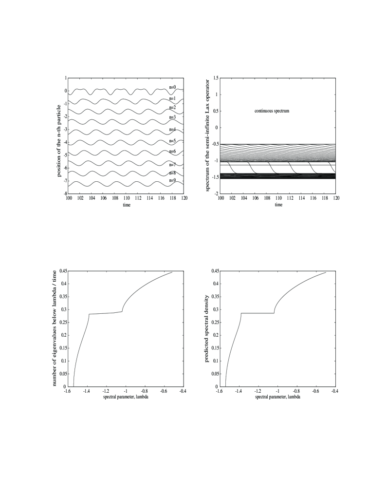
Figure C.12: Toda lattice with driver $x_{0}(t)=t+0.2\sin\gamma t+0.1\cos\gamma t,\gamma=1.8$, i.e. $\gamma_{1}>\gamma>\gamma_{2}$; see Section C.2 for detailed description.

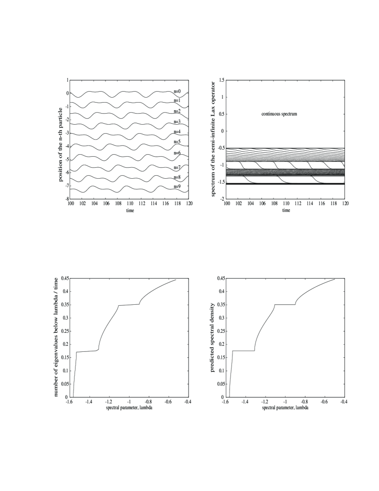
Figure C.13: Toda lattice with driver $x_{0}(t)=t+0.2\sin\gamma t+0.1\cos\gamma t,\gamma=1.1$, i.e. $\gamma_{2}>\gamma>\gamma_{3}$; see Section C.2 for detailed description.

Bibliography

• [A] N.I. Akhiezer, A continuous analogue to orthogonal polynomials on a system of intervals, Soviet Math. Dokl. 2 (1961), 1409-1412.
• [B] J. Bellisard, preprint.
• [BGGK] D.Battig, B. Grebert, J.-C. Guillot and T. Kappeler, Fibration of the phase space of the periodic Toda lattice, Preprint 1992.
• [BK] A. Bloch and T. Kodama, Dispersive regularization of the Whitham equation for the Toda lattice, SIAM J. Appl. Math., 52, (1992), 901-928.
• [BS] H.Behnke and F. Sommer, Theorie der analytischen Funktionen einer komplexen Veraenderlichen, Springer-Verlag, Berlin, 1965 (3).
• [CW] W. Craig and C. E. Wayne, Newton’s method and periodic solutions of nonlinear wave equations, Comm. Pure Appl. Math., 46, (1993), 1409-1498.
• [DT] E. Date and S. Tanaka, Analogue of Inverse Scattering Theory for the Discrete Hill’s Equation and Exact Solutions for the Periodic Toda Lattice, Prog. Theor. Phys. 55 (1976),457-465.
• [DMV] P. Deift, M. McDonald and S. Venakides, Renormalisation for the tau function for the Toda shock problem, in preparation.
• [D] B.A. Dubrovin, The inverse problem of scattering theory for periodic finite-zone potentials, Funct. Anal. Appl. 9:1 (1975), 65-66.
• [DMN] B.A. Dubrovin, V.B. Matveev and S.P. Novikov, Nonlinear equations of Korteweg-de Vries type, finite zone linear operators, and Abelian varieties, Russian Math. Surveys 31:1 (1976), 59-146.
• [FK] H. Farkas, I. Kra, Riemann Surfaces, Springer-Verlag, New York, 2nd ed., 1992.
• [F] H. Flaschka, The Toda lattice. I. Existence of integrals, Phys. Rev. B9, (1974), pp. 1924-1925. On the Toda lattice. II. Inverse scattering solution. Prog. Theor. Phys., 51, (1974), pp. 703-716.
• [FI] A. S. Fokas and A. R. Its, The linearization of the initial-boundary value problem of the nonlinear Schroedinger equation, Clarkson University, preprint 1993.
• [FW] G. Friesecke, J. A. D. Wattis, Existence Theorem for Solitary Waves on Lattices, preprint 1993.
• [G1] F. Gesztesy, Floquet Theory, private communication.
• [G2] F. Gesztesy, private communication.
• [GL] J. Goodman and P. D. Lax, On dispersive difference schemes I, Comm. Pure. Appl. Math., 41, (1988), 591-613.
• [GN] J. M. Greenberg and A. Nachman, Continuum limits for discrete gases with long and short range interactions, preprint 1993.
• [H] M. Henon, Integrals of the Toda lattice, Phys. Rev. B (3) , 9 (1974), 1921-1923.
• [HFM] B. L. Holian, H. Flaschka and D. W. McLaughlin, Shock waves in the Toda lattice: Analysis, Phys. Rev. A, 24, (1981), 2595-2623.
• [HS] B. L. Holian and G. K. Straub, Molecular dynamics of shock waves in one-dimensional chains, Phys. Rev. B 18, (1978), 1593-1608.
• [HL] T. Hou and P. D. Lax, Dispersive approximations in fluid dynamics, Comm. Pure. Appl. Math. 44, (1991), 1-40.
• [IM] A. R. Its and V. B. Matveev, On Hill operators with finitely many lacunae, Funct. Anal. Appl. 9:1 (1975), 69-70.
• [JM] R. Johnson and J. Moser, The rotation number for almost periodic potentials, Comm. Math. Phys. 84, (1982), pp. 403-438.
• [Kap] T. Kappeler, Fibration of the phase space for the Korteweg-de Vries equation, Ann. Inst. Fourier (Grenoble) 41 (1991), no. 3, 539-575.
• [Kam] S. Kamvissis, On the Long Time Behaviour of the Doubly Infinite Toda Lattice under Shock Initial Data, Ph.D. Thesis, Courant Institute (1991).
• [Kau] D. J. Kaup, The forced Toda lattice: An example of an almost integrable system, J. Math. Phys. 25 (2), (1984), 277-281.
• [KN] D. J. Kaup and D. H. Neuberger, The soliton birth rate in the forced Toda lattice, J. Math. Phys. 25 (2), (1984), 282-284.
• [Kr1] I.M. Krichever, Algebraic curves and nonlinear difference equations, Russian Math. Surveys 33:4 (1978), 255-256.
• [Kr2] I.M. Krichever, Algebro-geometric spectral theory of the Schroedinger difference operator and the Peierls model, Soviet Math. Dokl. 26 (1982), 194-198.
• [L] P.D. Lax, Integrals of nonlinear equations of evolution and solitary waves, Comm. Pure Appl. Math. 21 (1968), 467-490.
• [LL] P. D. Lax and C. D. Levermore, The small dispersion limit of the Korteweg-de Vries equation I, II, III, Comm. Pure Appl. Math. 36, (1983), pp. 253-290, 571-593, 809-829.
• [MW] W. Magnus, W. Winkler, Hill’s Equation, Interscience-Wiley, New York, 1966.
• [Man] S.V. Manakov, Complete integrability and stochastization of discrete dynamical systems, Zh. Eksper. Teoret. Fiz. 67 (1974), 543-555 (Russian); English trans. in Sov. Phys. JETP 40, (1975), pp. 269-274.
• [McKT] H.P. McKean and E. Trubowitz, Hill’s Operator and Hyperelliptic Function Theory in the Presence of Infinitely Many Branch Points, Comm. Pure Appl. Math. 29 (1976), 143-226.
• [Mos] J. Moser, Finitely many mass points on the line under the influence of an exponential potential-an integrable system, Dynamical Systems Theory and Applications, ed. J. Moser, Springer-Verlag, New York, 1975, 467-497.
• [RS1] M. Reed, B. Simon, Methods of modern mathematical physics I: Functional Analysis, Academic Press, New York, 1975.
• [RS2] M. Reed, B. Simon, Methods of modern mathematical physics IV: Analysis of Operators, Academic Press, New York, 1978.
• [S] B. Simon, preprint.
• [T1] M. Toda, Theory of nonlinear lattices, Springer-Verlag, Berlin, 1989, 2nd ed.
• [T2] M. Toda, J. Phys. Soc. Jpn. 22 (1967), 431.
• [V] S. Venakides, The Korteweg-de Vries equation with small dispersion: higher order Lax–Levermore theory, Comm. Pure Appl. Math. 43, (1990), pp. 335-361.
• [VDO] S. Venakides, P. Deift, R. Oba, The Toda Shock Problem, Comm. Pure Appl. Math. 44 (1991), 1171-1242.
• [WK] D. Wycoff and D. J. Kaup, Time evolution of the Scattering Data for the Forced Toda Lattice, Studies in Appl. Math. 81, (1989), 7-19.