Long term object drift forecast in the ocean with tide and wind

Abstract In this paper, we propose a new method to forecast the drift of objects in near coastal ocean on a period of several weeks. The proposed approach consists in estimating the probability of events linked to the drift using Monte Carlo simulations. It couples an averaging method which permits to decrease the computational cost and a statistical method in order to take into account the variability of meteorological loading factors.

Keywords Averaging method, Two scale modeling, Monte Carlo simulation, Wind time series, Ocean forecasting, Object drift

1 Introduction

Drift of things in the ocean is potentially dangerous for human activities and marine ecosystems. For instance, drifting containers may cause serious accidents in the event of collision with ships and oil spills may have very negative impacts especially in coastal areas. In this paper, we investigate a new method to forecast the drift of an object in near coastal ocean on a period of several weeks.

The motion of a drifting object on the sea surface is the net result of a number of forces acting upon it (water currents due to tide wave, atmospheric wind, wave motion, wave induced currents, gravitational force and buoyancy force). It is possible to estimate the drift trajectory given information on the local wind, the surface current, and the shape and the buoyancy of the object. For instance, in order to estimate the position of lost containers, the safety-and-rescue services generally use short-term meteorological forecasts as forcing of an hydrodynamic model of drift (see Daniel et al. [5]). It is usual in such problems to consider several possible buoyancy and drift properties for the object since these features are not known precisely in most cases. An uncertainty on the initial conditions (position and time) may also be taken into account (see Hackett et al. [13]).

Since we are interested in longer periods of time in the present study, we cannot directly use meteorological forecasts to estimate the object trajectory. Then the drift forecast has to be led out in terms of probability. This will be done using a Monte Carlo method, which makes it possible to estimate the probability of some scenarios linked to the object’s trajectory, like the probability of being in a given point at a given time or the probability of running aground in given areas, for example. It consists in computing the object trajectories corresponding to a large number of meteorological time series representative of the climatology on the considered area. Because of the variability of the meteorological conditions, it is necessary to compute a large number of trajectories in order to get reliable estimates of the quantities of interest. Hence we are faced with two problems.

At first, as the existing data sets describe the meteorological conditions only on the few last decades, it is necessary to be able to simulate new realistic meteorological time-series. For this, we have used stochastic models. More precisely, it is assumed that these time series can be decomposed as the sum of two components, the first one that describes the meteorological conditions at a synoptic scale and the second one that represents fluctuations at the smaller scale. Then, the synoptic component is simulated with a non-parametric resampling algorithm proposed by Monbet, Ailliot and Prevosto [15], and the short-term component with an Autoregressive model.

Secondly, we have to compute the corresponding object trajectories, which oscillate with tide, in a reasonable computational time. Indeed, the trajectory of a drifting object submitted to tide wave currents and currents generated by other meteorological factors, is essentially composed by a trend and oscillations due to the tide, which have a small period with respect to the time period of interest (several weeks). Due to these high frequency oscillations, the numerical integration of the considered system is generally time consuming. So that it is convenient to split the estimation of the displacement of the object in two steps: first, we calculate the trend which is of low computational cost thanks to the lack of oscillations and then we reconstruct the oscillation around the trend. For this, we apply the Averaging Method developed by Frénod [7] in order to identify the averaged fields governing the trend and the oscillating operators allowing the reconstruction of the real object trajectory from the trend. As far as we know, this method has never been used before in the metocean field.

In order to check the validity of the proposed methodology, we consider a situation with deterministic currents and negligible wave effects and we study a simplified model where the acceleration of the floating object is equal to the sum of the acceleration of the water (due to the wave tide and a perturbation of smaller order which represents other water currents) and the difference between the wind speed and the object velocity. This model is described more precisely in the second section. Then, in the third section, we present the basic ideas of the Averaging Method and we compare computational cost of this method with the one which consists in integrating the real trajectory directly. In Section 4, we validate our method using numerical experiments. First, the models of the meteorological forcing fields (tide wave, perturbation and wind) are specified. Then, the accuracy of the Averaging Method is checked on the basis of numerical comparisons. Finally, in Section 5 the methodology is illustrated with an example in which the probability of running aground is estimated for an academic domain.

2 Model

The model on which we shall implement the method evoked above is a very simplified model for large time drift in ocean, above continental shelf in strong tide zone, of an almost completely submerged object submitted to wind. This model is extracted from exhaustive scaling analysis for large time floating object drift which we shall present in a forthcoming paper.

In short, the evolution of the position $\mathbf{X}({t})=\mathbf{X}({t};{\mathbf{x}},{\mathbf{v}})$ $\in\mathbb{R}^{2}$ and the velocity $\mathbf{V}({t})=\mathbf{V}({t};{\mathbf{x}},{\mathbf{v}})$ $\in\mathbb{R}^{2}$ of the considered object, having ${\mathbf{x}}$ and ${\mathbf{v}}$ as initial position and velocity, is given by:

$$\displaystyle\frac{d\mathbf{X}}{d{t}} =\mathbf{V},$$ (2.1)

$$\displaystyle\frac{d\mathbf{V}}{d{t}} =\frac{d}{dt}\Big{[}\mathbf{m}({t},\mathbf{X}))\Big{]}+\Lambda(\mathbf{w}({t},\mathbf{X})-\mathbf{V})=\frac{\partial\mathbf{m}}{\partial{t}}({t},\mathbf{X})+\big{(}\nabla\mathbf{m}({t},\mathbf{X})\big{)}\mathbf{V}+\Lambda(\mathbf{w}({t},\mathbf{X})-\mathbf{V}),$$ (2.2)

where $\mathbf{m}\equiv\mathbf{m}({t},{\mathbf{x}})$ is the ocean velocity field and $\mathbf{w}\equiv\mathbf{w}({t},{\mathbf{x}})$ the wind velocity field. $\nabla\mathbf{m}$ stands for the Jacobian matrix of $\mathbf{m}$. This equation says nothing but that the object is submitted to the sea water acceleration and to the wind force quantified by a constant $\Lambda$.

The time scale ${\overline{t}}$ on which we want to observe the drift phenomenon is about 3 months and the object is submitted to tide oscillations whose period ${\overline{T}}$ is about 12.5 hours. Then a small parameter ${\varepsilon}$ appears in our problem: the ratio $\frac{{\overline{T}}}{{\overline{t}}}$ tide period on observation time scale. The magnitude of ${\varepsilon}$ is about $1/200$. We consider that the velocity measurement of the object, wind and water are all done with the same unit: ${\overline{v}}$. The observation length scale ${\overline{l}}$, which has to be the characteristic length of continental shelf, is about several hundred kilometers. This length has to be compared with the characteristic distance ${\overline{T}}{\overline{v}}$ the water covers during a tide period, which is of some kilometers. It seems then reasonable to consider that the ratio $\frac{{\overline{T}}{\overline{v}}}{{\overline{l}}}$ is also about ${\varepsilon}$.

Having those scale considerations at hand, we introduce the following rescaled variables $t^{\prime}$, ${\mathbf{x}}^{\prime}$ and ${\mathbf{v}}^{\prime}$ expressing time, position and velocity in unit ${\overline{t}}$, ${\overline{l}}$ and ${\overline{v}}$

$$t={\overline{t}}t^{\prime},{\mathbf{x}}={\overline{l}}{\mathbf{x}}^{\prime}\text{ and }{\mathbf{v}}={\overline{v}}{\mathbf{v}}^{\prime},$$ (2.3)

the rescaled trajectory $(\mathbf{X}^{\prime}(t^{\prime};{\mathbf{x}}^{\prime},{\mathbf{v}}^{\prime})$, $\mathbf{V}^{\prime}(t^{\prime};{\mathbf{x}}^{\prime},{\mathbf{v}}^{\prime}))$ defined by

$${\overline{l}}\mathbf{X}^{\prime}(t^{\prime};{\mathbf{x}}^{\prime},{\mathbf{v}}^{\prime})=\mathbf{X}({\overline{t}}t^{\prime};{\overline{l}}{\mathbf{x}}^{\prime},{\overline{v}}{\mathbf{v}}^{\prime}),~{}~{}~{}{\overline{v}}\mathbf{V}^{\prime}(t^{\prime};{\mathbf{x}}^{\prime},{\mathbf{v}}^{\prime})=\mathbf{V}({\overline{t}}t^{\prime};{\overline{l}}{\mathbf{x}}^{\prime},{\overline{v}}{\mathbf{v}}^{\prime}),$$ (2.4)

and the rescaled fields $\mathbf{m}^{\prime}$ and $\mathbf{w}^{\prime}$ defined by

$${\overline{v}}\mathbf{m}^{\prime}(t^{\prime},{\mathbf{x}}^{\prime})=\mathbf{m}({\overline{t}}t^{\prime},{\overline{l}}{\mathbf{x}}^{\prime}),~{}~{}~{}{\overline{v}}\mathbf{w}^{\prime}(t^{\prime},{\mathbf{x}}^{\prime})=\mathbf{w}({\overline{t}}t^{\prime},{\overline{l}}{\mathbf{x}}^{\prime}).$$ (2.5)

We consider that the sea velocity writes

$$\mathbf{m}^{\prime}(t^{\prime},{\mathbf{x}}^{\prime})=\mathbf{M}(t^{\prime},\frac{{\overline{t}}}{{\overline{T}}}t^{\prime},{\mathbf{x}}^{\prime})+{\varepsilon}\mathbf{N}(t^{\prime},\frac{{\overline{t}}}{{\overline{T}}}t^{\prime},{\mathbf{x}}^{\prime})=\mathbf{M}(t^{\prime},\frac{t^{\prime}}{{\varepsilon}},{\mathbf{x}}^{\prime})+{\varepsilon}\mathbf{N}(t^{\prime},\frac{t^{\prime}}{{\varepsilon}},{\mathbf{x}}^{\prime}),$$ (2.6)

where $\mathbf{M}({t}^{\prime},\frac{t^{\prime}}{{\varepsilon}},{\mathbf{x}}^{\prime})$ $\in\mathbb{R}^{2}$ is the rescaled sea water velocity exclusively due to the tide wave. It is supposed to be regular. Considering its dependency with respect to the oscillating time variable, we suppose that $\theta^{\prime}\mapsto\mathbf{M}({t}^{\prime},\theta^{\prime},{\mathbf{x}}^{\prime})$ is a $1-$periodic function satisfying $\displaystyle\int{\bf\diagup}\hskip 4.0pt\mathbf{M}({t}^{\prime},\theta^{\prime},{\mathbf{x}}^{\prime})\,d\theta^{\prime}=0$ where $\displaystyle\int{\bf\diagup}\hskip 4.0pt\mathbf{M}({t}^{\prime},\theta^{\prime},{\mathbf{x}}^{\prime})\,d\theta^{\prime}=\int_{0}^{1}\mathbf{M}({t}^{\prime},\theta^{\prime},{\mathbf{x}}^{\prime})\,d\theta^{\prime}$. The field ${\varepsilon}\mathbf{N}({t}^{\prime},\frac{t^{\prime}}{{\varepsilon}},{\mathbf{x}}^{\prime})$, where $\mathbf{N}({t}^{\prime},\theta^{\prime},{\mathbf{x}}^{\prime})$ is also $1-$periodic in $\theta^{\prime}$, is the sea water velocity perturbation induced by meteorological factors. As concerns the wind velocity field, we consider that $\mathbf{w}^{\prime}$ also involves two time scales, i.e.,

$$\mathbf{w}^{\prime}({t}^{\prime},{\mathbf{x}}^{\prime})=\mathbf{W}({t}^{\prime},\frac{t^{\prime}}{{\varepsilon}},{\mathbf{x}}^{\prime}).$$ (2.7)

Nonetheless, wind time series bring out as unrealistic considering a periodic dependency of $\mathbf{W}({t}^{\prime},\theta^{\prime},{\mathbf{x}}^{\prime})$ with respect to $\theta^{\prime}$. In practice, we only consider that, for any ${t}^{\prime}$ and ${\mathbf{x}}^{\prime}$, it admits an average value $\displaystyle\int{\bf\diagup}\hskip 4.0pt\mathbf{W}({t}^{\prime},\theta^{\prime},{\mathbf{x}}^{\prime})\,d\theta^{\prime}$ which actual definition is discussed later on.

Finally, we may deduce the equation satisfied by the rescaled trajectory and involving the rescaled fields. Removing the ^′, this equation, which is the model on which we shall implement our method, reads:

$$\frac{d\mathbf{X}}{d{t}}=\mathbf{V},$$ (2.8)

$$\begin{aligned} \frac{d\mathbf{V}}{d{t}}=\frac{1}{{\varepsilon}}\frac{\partial\mathbf{M}}{\partial\theta}({t},\frac{t}{{\varepsilon}},\mathbf{X})+\frac{\partial\mathbf{M}}{\partial{t}}({t},\frac{t}{{\varepsilon}},\mathbf{X})+\frac{\partial\mathbf{N}}{\partial\theta}({t},\frac{t}{{\varepsilon}},\mathbf{X})+\big{(}\nabla\mathbf{M}({t},\frac{t}{{\varepsilon}},\mathbf{X})\big{)}\mathbf{V}+\mathbf{W}({t},\frac{t}{{\varepsilon}},\mathbf{X})-\mathbf{V}~{}~{}~{}~{}&\\ +{\varepsilon}\Big{(}\frac{\partial\mathbf{N}}{\partial{t}}({t},\frac{t}{{\varepsilon}},\mathbf{X})+\big{(}\nabla\mathbf{N}({t},\frac{t}{{\varepsilon}},\mathbf{X})\big{)}\mathbf{V}\Big{)}.&\end{aligned}$$ (2.9)

Notice that system (2.8)-(2.9) is rescaled, and that, in it, every variable and field characteristic scale is of order 1.

Clearly, the model under consideration is too simplistic to be used for operational applications. Nevertheless, it contains most of the physical ingredients of drift of object in the ocean: joint action of sea and wind, two time scales, possibility of using not so unrealistic sea velocity fields. Moreover, it seems to be relatively straightforward to incorporate a realistic sea velocity in it, with a tide period that weakly evolves with time and to apply it in a real geographical geometry. Hence, the validity of the methodology we present in this paper is not limited by the simplifications we consider.

3 Asymptotic analysis

Having the goal of using the Monte Carlo Method to estimate the probability of events linked to the trajectory of the drifting object in mind, we need to compute the object trajectory for a large number of wind conditions. The solution $(\mathbf{X},\mathbf{V})$ contains $\frac{1}{{\varepsilon}}-$frequency oscillations. Then, solving (2.8)-(2.9) directly by numerical methods forces the use of a very small time step. For instance, if the explicit Euler scheme is used, since the characteristic size of the left hand side of (2.9) and of its gradient are about $\frac{1}{{\varepsilon}}$ and the size of its time derivative is about $\frac{1}{{\varepsilon}^{2}}$, the classical error estimate yields, for a time step $\Delta t$ small enough, an error about

$$\frac{\Delta t}{{\varepsilon}}\bigg{(}1+\frac{\Delta t}{{\varepsilon}}\bigg{)}^{\frac{1}{\Delta t}}\sim~{}\frac{\Delta t}{{\varepsilon}}e^{\frac{1}{{\varepsilon}}}.$$ (3.1)

Hence, if we want to obtain a precision about ${\varepsilon}^{2}$ a time step $\Delta t$ about ${\varepsilon}^{3}e^{-\frac{1}{{\varepsilon}}}$ is needed. This is really too small for operational applications. Hence we shall write an expansion of $(\mathbf{X},\mathbf{V})$ and find non oscillating equations satisfied by the terms of this expansion. This way, the previously evoked constraint imposed on the time step vanishes.

It is an easy game to see that system (2.8)-(2.9) enters the framework of an oscillatory-singularly perturbed dynamical system

$$\frac{d}{dt}\begin{pmatrix}\mathbf{X}\\ \mathbf{V}\end{pmatrix}=\mathbf{a}(t,\frac{t}{{\varepsilon}},\mathbf{X},\mathbf{V})+{\varepsilon}\mathbf{a}^{1}(t,\frac{t}{{\varepsilon}},\mathbf{X},\mathbf{V})+\frac{1}{{\varepsilon}}\mathbf{b}(t,\frac{t}{{\varepsilon}},\mathbf{X},\mathbf{V}),$$ (3.2)

very close to the one studied by Frénod [7] which originates from gyrokinetic plasma questions (see also Poincaré [17], Krylov and Bogoliubov [14], Bogoliubov and Mitropolsky [3], Sanders and Verhulst [19], Schochet [20], Frénod and Sonnendrücker [9, 10, 11], Frénod and Watbled [12] and Frénod, Raviart and Sonnendrücker [8] for presentations of methods allowing to remove time oscillations). With very little changes we may apply the results it contains to deduce that

$$\mathbf{X}(t)={\mathbf{X}^{0}}(t,\frac{t}{{\varepsilon}})+{\varepsilon}{\mathbf{X}^{1}}(t,\frac{t}{{\varepsilon}})+\dots,~{}~{}~{}~{}~{}~{}\mathbf{V}(t)=\mathbf{V}^{0}(t,\frac{t}{{\varepsilon}})+{\varepsilon}\mathbf{V}^{1}(t,\frac{t}{{\varepsilon}})+\dots,$$ (3.3)

where oscillating functions ${\mathbf{X}^{0}}$, $\mathbf{V}^{0}$, ${\mathbf{X}^{1}}$ and $\mathbf{V}^{1}$ are linked to non oscillating functions ${\mathbf{Y}^{0}}$, $\mathbf{U}^{0}$, ${\mathbf{Y}^{1}}$ and $\mathbf{U}^{1}$ by

$${\mathbf{X}^{0}}(t,\theta)={\mathbf{Y}^{0}}(t),$$ (3.4)

$$\mathbf{V}^{0}(t,\theta)=\mathbf{M}({t},\theta,{\mathbf{Y}^{0}}(t))+\mathbf{U}^{0}(t),$$ (3.5)

and

$${\mathbf{X}^{1}}(t,\theta)={\mathbf{Y}^{1}}(t)+\int_{0}^{\theta}\mathbf{M}({t},\sigma,{\mathbf{Y}^{0}}(t))\,d\sigma,$$ (3.6)

$$\begin{aligned} \mathbf{V}^{1}&(t,\theta)=\{\nabla\mathbf{M}({t},\theta,{\mathbf{Y}^{0}}(t))\}\{{\mathbf{Y}^{1}}(t)+\int_{0}^{\theta}\mathbf{M}({t},\sigma,{\mathbf{Y}^{0}}(t))\,d\sigma\}\\ \displaystyle&+\mathbf{U}^{1}(t)+\mathbf{N}({t},\theta,{\mathbf{Y}^{0}}(t))-\mathbf{N}({t},0,{\mathbf{Y}^{0}}(t))+\int_{0}^{\theta}\Big{(}\mathbf{W}({t},\sigma,{\mathbf{Y}^{0}}(t))-\int{\bf\diagup}\hskip 4.0pt\mathbf{W}({t},\varsigma,{\mathbf{Y}^{0}}(t))\,d\varsigma\Big{)}\,d\sigma\\ &-\int_{0}^{\theta}\mathbf{M}({t},\sigma,{\mathbf{Y}^{0}}(t))\,d\sigma.\end{aligned}$$ (3.7)

Then ${\mathbf{Y}^{0}}$, $\mathbf{U}^{0}$, ${\mathbf{Y}^{1}}$ and $\mathbf{U}^{1}$ are the solution to

$$\frac{d{\mathbf{Y}^{0}}}{dt}=\mathbf{U}^{0},$$ (3.8)

$$\frac{d\mathbf{U}^{0}}{dt}=\int{\bf\diagup}\hskip 4.0pt\mathbf{W}({t},\theta,{\mathbf{Y}^{0}})\,d\theta-\mathbf{U}^{0},$$ (3.9)

$$\begin{aligned} \frac{d{\mathbf{Y}^{1}}}{dt}&=\displaystyle\int{\bf\diagup}\hskip 4.0pt\{\nabla\mathbf{M}({t},\theta,{\mathbf{Y}^{0}})\}\{\int_{0}^{\theta}\mathbf{M}({t},\sigma,{\mathbf{Y}^{0}})\,d\sigma\}\,d\theta\\ \displaystyle&+\mathbf{U}^{1}+\int{\bf\diagup}\hskip 4.0pt\mathbf{N}({t},\theta,{\mathbf{Y}^{0}})\,d\theta-\mathbf{N}({t},0,{\mathbf{Y}^{0}})+\int{\bf\diagup}\hskip 4.0pt\int_{0}^{\theta}\Big{(}\mathbf{W}({t},\sigma,{\mathbf{Y}^{0}})-\int{\bf\diagup}\hskip 4.0pt\mathbf{W}({t},\varsigma,{\mathbf{Y}^{0}})\,d\varsigma\Big{)}d\sigma\,d\theta\\ &-\int{\bf\diagup}\hskip 4.0pt\int_{0}^{\theta}\mathbf{M}({t},\sigma,{\mathbf{Y}^{0}})\,d\sigma d\theta-\Big{\{}\int{\bf\diagup}\hskip 4.0pt\int_{0}^{\theta}\nabla\mathbf{M}({t},\sigma,\mathbf{y}^{0})\,d\sigma d\theta\Big{\}}\{\mathbf{U}^{0}\}-\int{\bf\diagup}\hskip 4.0pt\int_{0}^{\theta}\frac{\partial\mathbf{M}}{\partial{t}}({t},\sigma,\mathbf{y}^{0})\,d\sigma d\theta,\end{aligned}$$ (3.10)

$$\begin{aligned} \frac{d\mathbf{U}^{1}}{dt}&=\displaystyle\big{\{}\int{\bf\diagup}\hskip 4.0pt\nabla\mathbf{W}({t},\theta,{\mathbf{Y}^{0}})d\theta\big{\}}\{{\mathbf{Y}^{1}}\}+\int{\bf\diagup}\hskip 4.0pt\big{\{}\nabla\mathbf{W}({t},\theta,{\mathbf{Y}^{0}})\big{\}}\big{\{}\int_{0}^{\theta}\mathbf{M}({t},\sigma,{\mathbf{Y}^{0}})\,d\sigma\big{\}}d\theta\\ &-\Big{\{}\int{\bf\diagup}\hskip 4.0pt\{\nabla\mathbf{M}({t},\theta,{\mathbf{Y}^{0}})\}\{\int_{0}^{\theta}\mathbf{M}({t},\sigma,{\mathbf{Y}^{0}})\,d\sigma\}d\theta+\mathbf{U}^{1}+\int{\bf\diagup}\hskip 4.0pt\mathbf{N}({t},\theta,{\mathbf{Y}^{0}})\,d\theta-\mathbf{N}({t},0,{\mathbf{Y}^{0}})\\ &+\int{\bf\diagup}\hskip 4.0pt(\int_{0}^{\theta}\mathbf{W}({t},\sigma,{\mathbf{Y}^{0}})\,d\sigma-\theta\int{\bf\diagup}\hskip 4.0pt\mathbf{W}({t},\sigma,{\mathbf{Y}^{0}})\,d\sigma)\,d\theta-\int{\bf\diagup}\hskip 4.0pt\int_{0}^{\theta}\mathbf{M}({t},\sigma,{\mathbf{Y}^{0}})\,d\sigma d\theta\Big{\}}\\ \displaystyle&+\Big{\{}\nabla\mathbf{N}({t},0,{\mathbf{Y}^{0}})\\ \displaystyle&-\int{\bf\diagup}\hskip 4.0pt\nabla\Big{(}\int_{0}^{\theta}\mathbf{W}(\cdot,\sigma,\cdot)\,d\sigma-\theta\int{\bf\diagup}\hskip 4.0pt\mathbf{W}(\cdot,\sigma,\cdot)\,d\sigma\Big{)}({t},{\mathbf{Y}^{0}})\,d\theta+\int{\bf\diagup}\hskip 4.0pt\int_{0}^{\theta}\mathbf{M}({t},\sigma,{\mathbf{Y}^{0}})\,d\sigma d\theta\Big{\}}\{\mathbf{U}^{0}\}\\ \displaystyle&+\frac{\partial\mathbf{N}}{\partial t}({t},0,{\mathbf{Y}^{0}})-\int{\bf\diagup}\hskip 4.0pt\frac{\partial\displaystyle\Big{(}\int_{0}^{\theta}\mathbf{W}(\cdot,\sigma,\cdot)\,d\sigma-\theta\int{\bf\diagup}\hskip 4.0pt\mathbf{W}(\cdot,\sigma,\cdot)\,d\sigma\Big{)}}{\partial t}({t},{\mathbf{Y}^{0}})\,d\theta\\ \displaystyle&~{}~{}~{}~{}~{}~{}~{}~{}~{}~{}~{}~{}~{}~{}~{}~{}~{}~{}~{}~{}~{}~{}~{}~{}~{}~{}~{}~{}~{}~{}~{}~{}~{}~{}~{}~{}~{}~{}~{}~{}~{}~{}~{}~{}~{}~{}~{}~{}~{}~{}~{}~{}~{}~{}~{}~{}~{}~{}~{}~{}~{}~{}~{}~{}~{}~{}~{}~{}~{}~{}~{}~{}~{}~{}~{}~{}~{}~{}~{}~{}~{}~{}+\int{\bf\diagup}\hskip 4.0pt\int_{0}^{\theta}\frac{\partial\mathbf{M}}{\partial t}({t},\sigma,{\mathbf{Y}^{0}})\,d\sigma d\theta,\end{aligned}$$ (3.11)

equipped with initial conditions ${\mathbf{Y}^{0}}(0)={\mathbf{x}}$, $\mathbf{U}^{0}(0)={\mathbf{v}}$, ${\mathbf{Y}^{1}}(0)=0$ and $\mathbf{U}^{1}(0)=0$.

As said previously, this result may be inferred from [7]. It may also be deduced by expanding fields and functions in (2.8) and (2.9) in a correct way. This is done formally in the Appendix.

Equations (3.4) and (3.5) mean that the order 0 trajectory does not oscillate and that the 0 order velocity is the tide velocity added with a non oscillating velocity $\mathbf{U}^{0}$ which is generated by wind. Wind acts on $\mathbf{U}^{0}$ only through its averaged value. This is translated in (3.9). By the way, notice that since the average value of $\mathbf{M}$ is $0$, equations (3.8)-(3.9) only involve the average wind. As concerns order 1 terms, the situation is more complex. First since $\int_{0}^{\theta}\mathbf{M}({t},\sigma,{\mathbf{Y}^{0}}(t))\,d\sigma$ may be interpreted as the position of a sea water particle placed in ${\mathbf{Y}^{0}}(t)$ at the beginning of a tide cycle ($\theta=0$), equation (3.6) means that the order 1 position is this water particle position plus a non oscillating function ${\mathbf{Y}^{1}}(t)$. Regarding the terms (3.7) contains, the first one describes the way the space variation of the tide velocity acts, the second one is the non oscillating part of the velocity. The third and fourth terms quantify the action of the sea velocity perturbation. Concerning the next term, we need to remember that the action of the averaged value of the wind velocity is taken into account in order 0 equation (3.9). Then we notice that $\mathbf{W}({t},\sigma,{\mathbf{Y}^{0}}(t))-\int{{\scriptscriptstyle\bf\diagup}}\hskip 4.0pt\mathbf{W}({t},\varsigma,{\mathbf{Y}^{0}}(t))$ quantifies the wind action around its averaged value at each time of a tide cycle. Hence $\int_{0}^{\theta}\Big{(}\mathbf{W}({t},\sigma,{\mathbf{Y}^{0}}(t))-\int{{\scriptscriptstyle\bf\diagup}}\hskip 4.0pt\mathbf{W}({t},\varsigma,{\mathbf{Y}^{0}}(t)))\,d\varsigma\Big{)}\,d\sigma$ is the cumulated action of the wind around its averaged value. This quantity acts at order 1. The last term of (3.7) can be interpreted as the previous one recalling that the mean value of the sea velocity is 0. It is hard to give intuitive explanations for the evolution equations (3.10)-(3.11). We only notice that they involve mean value of non-linear interactions between fields which quantify the mean joint action of sea and wind. This non intuitive quantification is made possible thanks to the asymptotic analysis presented in [7] and in the Appendix.

The characteristic size of the right hand sides in (3.8)-(3.11) are 1. Hence, to get the same precision about ${\varepsilon}^{2}$, with the same Euler scheme using (3.3)-(3.11) to compute $(\mathbf{X},\mathbf{V})$, in place of using (2.8)-(2.9) as evoked in the beginning of this section, the needed time step $\Delta t$ is about ${\varepsilon}^{2}$. Comparing this with the value ${\varepsilon}^{3}e^{-\frac{1}{{\varepsilon}}}$ found in the beginning of the section, despite the heavy form of (3.8)-(3.11), this is an appreciable gain even more so given that our probabilistic forecast method needs numbers of simulations for numbers of wind time series.

Concerning the validity of the expansion (3.3), if $\mathbf{W}({t},\theta,{\mathbf{x}})$ was a regular function, periodic with respect to $\theta$, asymptotic expansion (3.3) could be rigorously justified, applying [7], by the following inequality

$$\sup_{t\in[0,1]}\|\mathbf{X}(t)-{\mathbf{X}^{0}}(t,\frac{t}{{\varepsilon}})\|\leq c{\varepsilon},~{}\sup_{t\in[0,1]}\|\mathbf{X}(t)-{\mathbf{X}^{0}}(t,\frac{t}{{\varepsilon}})-{\varepsilon}{\mathbf{X}^{1}}(t,\frac{t}{{\varepsilon}})\|\leq c{\varepsilon}^{2},$$ (3.12)

$$\sup_{t\in[0,1]}\|\mathbf{V}(t)-\mathbf{V}^{0}(t,\frac{t}{{\varepsilon}})\|\leq c{\varepsilon},~{}\sup_{t\in[0,1]}\|\mathbf{V}(t)-\mathbf{V}^{0}(t,\frac{t}{{\varepsilon}})-{\varepsilon}\mathbf{V}^{1}(t,\frac{t}{{\varepsilon}})\|\leq c{\varepsilon}^{2},$$ (3.13)

which would be true for ${\varepsilon}$ small enough and for a constant $c$ independent of ${\varepsilon}$, where $\|\cdot\|$ stands for the Euclidean norm in $\mathbb{R}^{2}$.

As we cannot consider the wind time series to have this form, we will estimate the error using numerical experiments. This is done in the next section: several realistic wind time series are simulated using a method described in Monbet et al. [15] and the corresponding error is calculated for each of them. For this, we have to decide how the average values are to be computed. If the way is clear for fields linked to $\mathbf{M}$ or $\mathbf{N}$, for which we simply take $\int{{\scriptscriptstyle\bf\diagup}}\hskip 4.0ptd\theta=\int_{0}^{1}d\theta$, the situation is more obscure for wind linked fields. For them, we will take as averaged value at time $t$ the mean value on the interval centered in $t$ and with length $p$, i.e.

$$\int{\bf\diagup}\hskip 4.0pt\mathbf{W}({t},\theta,{\mathbf{x}})\,d\theta=\frac{1}{p}\int_{t-p/2}^{t+p/2}\mathbf{W}(s,\frac{s}{{\varepsilon}},{\mathbf{x}})\,ds,$$ (3.14)

for a parameter $p$ that has to be adjusted experimentally. As concerns the integrals in $\theta$ of the wind linked fields, they have to be replaced by integrals respecting $\mathbf{V}_{1}(t,\frac{t}{{\varepsilon}})=\mathbf{U}_{1}(t)$ when $\frac{t}{{\varepsilon}}$ is an integer, which is a constraint imposed by the Averaging Method. Hence, we replace

$$\bigg{(}\int_{0}^{\theta}\mathbf{W}({t},\sigma,{\mathbf{x}})\,d\sigma\bigg{)}_{|\theta=\frac{t}{{\varepsilon}}}\text{ ~{} by ~{} }\int_{{\varepsilon}[\frac{t}{{\varepsilon}}]}^{t}\mathbf{W}(s,\frac{s}{{\varepsilon}},{\mathbf{x}})\,ds,$$ (3.15)

where $[\frac{t}{{\varepsilon}}]$ stands for the integer part of $\frac{t}{{\varepsilon}}$. Those choices have also to be experimentally validated.

4 Numerical validation

We begin this section by introducing the sea velocity fields and briefly presenting the stochastic method used to generate the wind time series. Then, the expansion (3.3) is validated by numerical experiments. More precisely, several wind time series are generated. Then, for each of them, we compute the real trajectory using (2.8)-(2.9) and compare it to the trajectory obtained with expansion (3.3) and the following equations.

4.1 Metocean fields

Let us first describe the metocean fields that have been used in our numerical experiments. Regarding the rescaled ocean velocity induced by the tide wave and its perturbation, we have chosen the following simple parametric fields:

$$\mathbf{M}(t,\theta,{\mathbf{x}})=(2+\sin(6\pi t))~{}x_{1}\begin{pmatrix}\sin(2\pi\theta)+\frac{1}{4}\sin(4\pi\theta)\\ \frac{1}{2}\sin(2\pi\theta)\end{pmatrix},$$ (4.1)

$$\mathbf{N}(t,\theta,{\mathbf{x}})=(2+\cos(6\pi t))~{}x_{2}\begin{pmatrix}\sin(2\pi\theta)\\ \sin(2\pi\theta)\end{pmatrix},$$ (4.2)

where $x_{1}$ and $x_{2}$ are the first and second components of ${\mathbf{x}}$.

The trajectories associated with the field $\begin{pmatrix}\sin(2\pi\theta)+\frac{1}{4}\sin(4\pi\theta)\\ \frac{1}{2}\sin(2\pi\theta)\end{pmatrix}$ are non circular loops which remind those we can observe in Nihoul [16] or Salomon and Breton [18]. The velocity field $\mathbf{M}$ is this simple vector field modulated by a time and position dependency in order to see the influence of time derivative and gradient on the object trajectory. $\mathbf{N}$ is also a simple field which gradient is orthogonal to the one of $\mathbf{M}$.

In order to simulate realistic wind time series, we have assumed that they can be decomposed as the sum of two components, e.g $\mathbf{W}(t,\frac{t}{{\varepsilon}},{\mathbf{x}})=\mathbf{W}_{Lt}(t,{\mathbf{x}})+\mathbf{W}_{st}(\frac{t}{{\varepsilon}},{\mathbf{x}})$ where

• $\mathbf{W}_{Lt}(t,{\mathbf{x}})$ represents the wind evolution at a synoptic-scale, e.g at the scale of the high- and low-pressure systems. The typical dimension of these systems ranges approximately from 1000km and 2500km and their duration is a couple of days to at most a couple of weeks.

• $\mathbf{W}_{st}(\frac{t}{{\varepsilon}},{\mathbf{x}})$ represents the small scale evolution of the wind (e.g mesoscale and microscale winds). This scale includes phenomena such as thunderstorms, squall lines, land and sea breezes…

Such a decomposition is discussed more precisely by Breckling (see Breckling [4] and [1]). Different methods have been proposed in the literature to simulate realistic wind time-series at the synoptic scale (see Monbet, Ailliot and Prevosto [15] and references therein). In this study, we have first assumed that the wind $\mathbf{W}_{Lt}(t,x)$ is homogeneous in space; i.e. $\mathbf{W}_{Lt}(t,x)=\mathbf{W}_{Lt}(t)$ for all ${\mathbf{x}}$ and $t$, what seems realistic according the size of the domain which is supposed to be about some hundred kilometers. Then, we have used a non-parametric resampling method to simulate the process $\mathbf{W}_{Lt}(t)$, namely the Local Grid Bootstrap algorithm proposed by Monbet, Ailliot and Prevosto [15]. This method has already been validated on various datasets, and it was found that it can successfully be used to simulate realistic wind time series. In the present study, it has been calibrated on a dataset which describes the wind condition during the summer at a point of coordinates $(46.25\,N,1.67\,W)$, located near the French Atlantic coast. It describes the synoptic wind conditions during the last 20 years recorded every $\Delta t_{1}=6$ hours.

Then, in order to simulate the small scale variations, we have used an Autoregressive model. More precisely, for simplicity reasons, we have first assumed that this field is homogeneous in space. This assumption is unrealistic and could be refined later on. Then, we have assumed that, for $k\in\mathbb{N}^{*}$,

$$\mathbf{W}_{st}(k\Delta t_{2})=a\mathbf{W}_{st}((k-1)\Delta t_{2})+E(k\Delta t_{2})$$ (4.3)

where $\{E(k\Delta t_{2})\}_{k\in\mathbb{N}^{*}}$ denotes a zero-mean Gaussian white noise with covariance matrix $\sigma^{2}I_{2}$. In practice, we have simulated this small-scale component with a time-step $\Delta t_{2}={\varepsilon}/100$. This consists in giving the wind value every $4$ min approximately, and the parameters $a$ and $\sigma$ have been chosen such that the process $\mathbf{W}_{st}$ has a memory of a few hours and such that the standard deviation of its marginal distribution represents approximately $10\%$ of the one of the process $\mathbf{W}$.

Finally, the procedure described above makes it possible to simulate the processes $\mathbf{W}_{Lt}(t)$ and $\mathbf{W}_{st}(\frac{t}{{\varepsilon}})$ for $t\in k\Delta t_{1}$ and $\frac{t}{{\varepsilon}}\in k\Delta t_{2}$, respectively. The values of these processes for other values of $t$ have been calculated by linear extrapolation. An example of simulated wind time-series is given in Figure 2.

4.2 Numerical results

In order to validate the asymptotic expansion given in the previous section, we have computed the solutions of (2.8)-(2.9) and of (3.3)-(3.11) for $N=100$ artificial wind time series. Let us denote $\hat{\mathbf{X}}_{i}$, $\hat{\mathbf{V}}_{i}$, $\hat{\mathbf{X}}_{i}^{0}$, $\hat{\mathbf{V}}_{i}^{0}$, $\hat{\mathbf{X}}_{i}^{1}$, $\hat{\mathbf{V}}_{i}^{1}$, for $i\in\{1,...,N\}$, the corresponding numerical approximations of $\mathbf{X}$, $\mathbf{V}$, $\mathbf{X}^{0}$, $\mathbf{V}^{0}$, $\mathbf{X}^{1}$ and $\mathbf{V}^{1}$, respectively. We have tested different algorithms to solve these ODEs, and the best results have been obtained with an explicit Runge-Kutta (4,5) formula. In practice, we have used the Maltlab’s function ode45 which is based on an explicit Runge-Kutta (4,5) formula, the Dormand-Prince pair [6]. In the numerical results given hereafter, we have used ${\varepsilon}=1/50$. This choice makes it possible to compute the solutions of the system (2.8)-(2.9) with a good precision in a reasonable computational time, and permits also easier graphics representations. We have used ${\mathbf{x}}_{i}=(1,1)$ and ${\mathbf{v}}_{i}=(0,0)$ as initial values.

In Table 1, the norms of error in object position and velocity for order 0 and 1 expansions are given. Let us discuss more precisely the results obtained with $\epsilon=1/50$. It shows that the asymptotic expansions obtained with $p={\varepsilon}/10$ (corresponding to an interval of $40$ min), $p={\varepsilon}/2$ (corresponding to an interval of $6\textrm{h}15\textrm{min}$) and $p={\varepsilon}$ (corresponding to an interval of $12\textrm{h}30\textrm{min}$) are about $5{\varepsilon}^{2}$ worth, and close to each other. For comparison, we also compute the solution to system (3.3)-(3.11) when the wind is null, and we also found an error equal to $0.0022\approx 5{\varepsilon}^{2}$. For $p=4{\varepsilon}$ (corresponding to an interval of $2$ days), the error is significantly higher. As concerns the computational coast, it decreases as $p$ increases, so that a good compromise seems to use ${\varepsilon}/2\leq p\leq{\varepsilon}$; i.e. the wind at a synoptic scale. Such a value of $p$ permits to compute the solutions of the system (3.3)-(3.11) with a good precision in a computational time significantly lower than the one corresponding to the system (2.8)-(2.9). For instance, if an Euler scheme is used, the exact system (2.8)-(2.9) requires about 1000 more iterations than the approximate system (3.3)-(3.11) to achieve the same accuracy. And, for the problem considered in this paper, an iteration of the exact system is 20 less expensive in terms of computational time. But this last remark is not general since the computational time highly depends on the nature of the tide and current fields $M$ and $N$ : here they are modeled by a quite simple analytical formula.

In Figure 1, we have plotted the object trajectory associated with the wind time series shown on the top of Figure 2, using $p={\varepsilon}/2$. More precisely, the solid line represent $\hat{\mathbf{X}}$ computed by directly solving (2.8)-(2.9). The dashed line represents the average trajectory $\hat{\mathbf{Y}}^{0}+{\varepsilon}\hat{\mathbf{Y}}^{1}$ obtained solving (3.8) and (3.10). We can see that this averaged trajectory follows nicely the trend of $\hat{\mathbf{X}}$. Then reconstructing $\hat{\mathbf{X}}^{0}$ and $\hat{\mathbf{X}}^{1}$ using (3.4) and (3.6), we have represented the trajectory $\hat{\mathbf{X}}^{0}+{\varepsilon}\hat{\mathbf{X}}^{1}$ in dotted line. The superimposition with $\hat{\mathbf{X}}$ seems to be almost perfect. In order to go further in the result analysis, we turn to Figure 2. On the top of this figure, we have shown the wind as a function of time. The second figure represents, in dashed line, the average trajectory of the position of the first component and, in solid line, the first component of the trajectory itself. We can see on this trajectory not only the long term trend but also the two time periodic phenomena in game: tide oscillations (rapid oscillations) and tide coefficient amplitude (modulated amplitude). Finally, the last plot exhibit ${\varepsilon}^{2}-$order error (here ${\varepsilon}=1/50=2.\,10^{-2}$, then $10^{-3}=2.5\,{\varepsilon}^{2}$). Moreover, we can see that this error function is a periodic function with modulated amplitude. This spurs us thinking that we could improve the accuracy of the reconstructed trajectory, if it is needed, considering the next terms in the expansion of $\mathbf{X}$ and $\mathbf{V}$. Figure 3 shows the first component of the average wind, the average velocity (dashed line) and the velocity itself (solid line). The third plot shows the error on the velocity. This figure permits to visualize the action of the wind on the averaged velocity, which first increases and then decreases.

In order to make our numerical validation more convincing, we also made simulations for varying ${\varepsilon}$. In Table 2, the norms of the error on object position and velocity for order 0 and 1 expansions are given for ${\varepsilon}=1/100$ and ${\varepsilon}=1/25$ . The errors are proportional to ${\varepsilon}$ for order 0 and to ${\varepsilon}^{2}$ for order 1 as it was expected from the theory.

${\varepsilon}=\frac{1}{50}$ Speed (order 0) Speed (order 1) Position (order 0) Position (order 1) $p=\frac{{\varepsilon}}{10}$ 0.1115 [0.1115,0.1116] 0.0460 [0.0454,0.0467] 0.0174 [0.0173,0.0174] 0.0023 [0.0021,0.0029] $p=\frac{{\varepsilon}}{2}$ 0.1118 [0.1113,0.1134] 0.0460 [0.0448,0.0473] 0.0174 [0.0173,0.0174] 0.0024 [0.0021,0.0032] $p={\varepsilon}$ 0.1125 [0.1108,0.1168] 0.0460 [0.0441,0.0488] 0.0173 [0.0171,0.0174] 0.0026 [0.0020,0.0047] $p=4{\varepsilon}$ 0.1192 [0.1102,0.1280] 0.0542 [0.0438,0.0691] 0.0174 [0.0166,0.0196] 0.0065 [0.0024,0.0144] $W\equiv 0$ 0.1115 0.0096 0.0174 0.0022

Table 1: Mean value, minimum and maximum values (mean [min, max]) of the errors $\sup_{t\in[0,1]}\|\hat{\mathbf{V}}_{i}(t)-\hat{\mathbf{V}}_{i}^{0}(t)\|$ (second column), $\sup_{t\in[0,1]}\|\hat{\mathbf{V}}_{i}(t)-\hat{\mathbf{V}}_{i}^{0}(t)-{\varepsilon}\hat{\mathbf{V}}_{i}^{1}(t)\|$ (third column), $\sup_{t\in[0,1]}\|\hat{\mathbf{X}}_{i}(t)-\hat{\mathbf{X}}_{i}^{0}(t)\|$ (forth column) and $\sup_{t\in[0,1]}\|\hat{\mathbf{X}}_{i}(t)-\hat{\mathbf{X}}_{i}^{0}(t)-{\varepsilon}\hat{\mathbf{X}}_{i}^{1}(t)\|$ (fifth column) for different values of $p$. The last line for ${\varepsilon}=\frac{1}{50}$ gives the error for a zero wind field.

$\epsilon=\frac{1}{100}$ Speed (order 0) Speed (order 1) Position (order 0) Position (order 1) $p=\frac{{\varepsilon}}{10}$ 0.0557 [0.0557,0.0557] 0.0292 [0.0270,0.0358] 0.0086 [0.0085,0.0086] 0.0011 [ 0.0011,0.0014] $p=\frac{{\varepsilon}}{2}$ 0.0558 [0.0554,0.0563] 0.0294 [0.0270,0.0362] 0.0086 [0.0085,0.0086] 0.0012 [0.0010,0.0015] $p={\varepsilon}$ 0.0560 [0.0552,0.0574] 0.0296 [0.0273,0.0363] 0.0085 [0.0084,0.0086] 0.0013 [0.0010,0.0020] $p=4{\varepsilon}$ 0.0595 [0.0552,0.680] 0.0355 [0.0304,0.0516] 0.0086 [0.0082,0.0098] 0.0026 [0.0010,0.0072] ${\varepsilon}=\frac{1}{25}$ Speed (order 0) Speed (order 1) Position (order 0) Position (order 1) $p=\frac{{\varepsilon}}{10}$ 0.2254 [0.2249, 0.2257] 0.1143 [0.1022 ,0.1418] 0.0358 [0.0358,0.0359] 0.0046 [0.0040,0.0057] $p=\frac{{\varepsilon}}{2}$ 0.2254 [0.2226,0.2277] 0.1142 [0.1017,0.1410] 0.0358 [0.0357,0.0359] 0.0045 [0.0039,0.0058] $p={\varepsilon}$ 0.2257 [0.2201,0.2310] 0.1142 [0.1011,0.1379] 0.0358 [0.0356,0.0360] 0.0044 [0.0037,0.0069]

Table 2: Mean value, minimum and maximum values (mean [min, max]) of the errors $\sup_{t\in[0,1]}\|\hat{\mathbf{V}}_{i}(t)-\hat{\mathbf{V}}_{i}^{0}(t)\|$ (second column), $\sup_{t\in[0,1]}\|\hat{\mathbf{V}}_{i}(t)-\hat{\mathbf{V}}_{i}^{0}(t)-{\varepsilon}\hat{\mathbf{V}}_{i}^{1}(t)\|$ (third column), $\sup_{t\in[0,1]}\|\hat{\mathbf{X}}_{i}(t)-\hat{\mathbf{X}}_{i}^{0}(t)\|$ (forth column) and $\sup_{t\in[0,1]}\|\hat{\mathbf{X}}_{i}(t)-\hat{\mathbf{X}}_{i}^{0}(t)-{\varepsilon}\hat{\mathbf{X}}_{i}^{1}(t)\|$ (fifth column) for different values of $p$.

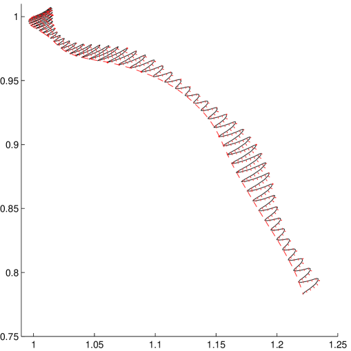
Figure 1: Example of object’s trajectory (two-dimensional phase plane plot). Solid line: $\hat{\mathbf{X}}$, Dotted line: $\hat{\mathbf{X}}^{0}+{\varepsilon}\hat{\mathbf{X}}^{1}$, Dashed line: $\hat{\mathbf{Y}}^{0}+{\varepsilon}\hat{\mathbf{Y}}^{1}$. ${\varepsilon}=1/50,p={\varepsilon}/2$.

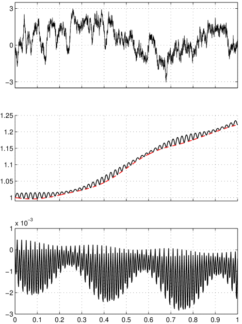
Figure 2: Example of object’s trajectory (time series plot)(Top: zonal wind first component, Second: first component of zonal object position (Solid line: $\hat{\mathbf{X}}$, Dashed line: $\hat{\mathbf{Y}}^{0}+{\varepsilon}\hat{\mathbf{Y}}^{1}$), Third: zonal error $\|\hat{\mathbf{X}}-\hat{\mathbf{X}}^{0}-{\varepsilon}\hat{\mathbf{X}}^{1}\|$). ${\varepsilon}=1/50,p={\varepsilon}/2$

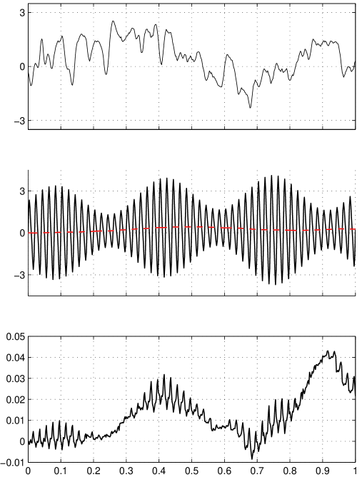
Figure 3: Example of object’s speed (time series plot)(Top: smoothed zonal wind component ($p=\epsilon/2$), Second: first component of zonal object’s speed (Solid line: $\hat{\mathbf{V}}$, Dashed line: $\hat{\mathbf{U}}^{0}+{\varepsilon}\hat{\mathbf{U}}^{1}$), Third: zonal error $\|\hat{\mathbf{V}}-\hat{\mathbf{V}}^{0}-{\varepsilon}\hat{\mathbf{V}}^{1}\|$). ${\varepsilon}=1/50,p={\varepsilon}/2$

5 Application: long term forecast of an object’s drift with Monte Carlo Method

In the previous section, we have shown that the expansion of the trajectories of an object in near coastal ocean submitted to wind makes it possible for us to compute quickly good approximation of this trajectory. It is then possible to make this computation for a large number of synthetic wind time series, and thus deduce the probability of a given scenario (this may be the probability of presence in a given area, of collision or of running aground, for example).

As an example, in this section we compute a running aground probability. More precisely, we have fixed an arbitrary coast line, e.g. the circle of center $(1,1)$ and radius $0.3$ and we have focused on the running aground of the object on this coast. We have generated one thousand wind time series with the same stochastic model as in the previous section and have also used the same sea velocity fields. We have computed the thousand associated trajectory. For this, we have used the method described in the previous sections, based on asymptotic expansion (3.3). The methodology is illustrated in Figure 4 where one hundred of the thousand trajectories are drawn. Proceeding this way, we have obtained enough trajectories to get reliable estimates of the quantities of interest. First we can deduce an estimation of the probability of running aground by calculating the percentage of trajectories that reach the circle in the time interval $[0,1]$. We found $64.3\%$. Then we can estimate the probability that the object runs aground in a given area. The obtained results are shown in Figure 5. On the left, we have plotted a wind rose which shows the joint repartition of direction and intensity. The length of each bar is proportional to the proportion of wind having a direction around the direction the bar indicates. The bars are then shared into four subbars which lengths are proportional to the proportion of wind having the corresponding magnitude. We can see that the wind is generally blowing from the north. The second histogram must be read in the following way. The length of each bar is proportional to the proportion of trajectories that run aground around the point of the coast which is in the bar direction. We then see that the proportion of running aground trajectories has a maximum around the South-South-West of the coast line.

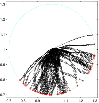
Figure 4: Object’s trajectory corresponding to 100 synthetic wind time series and corresponding running aground points(*)

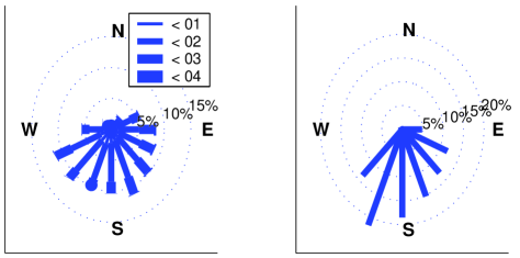
Figure 5: Repartition of the wind (left) and of the running aground points (right)

6 Conclusion

In this paper, we have explored a method to make probabilistic forecasts of long term drift, in near coastal ocean, of object submitted to tide and wind. The method is based on generating a large number of realistic wind time series and, for each of them, to compute the associated object trajectory. The probabilities of trajectory linked events may then be estimated using this large number of trajectory realizations. In order to achieve this goal, we have used a method proposed by Monbet, Ailliot and Prevosto [15] to generate realistic wind time series and the Averaging Method based on an asymptotic expansion of trajectory of Frénod [7] to remove tide oscillations and compute quickly the object’s trajectory. This method has allowed us to compute the probability for an object to run aground on an academic domain.

The quality of the results are good enough for us to contemplate going further in exploring this new methodology. Among the things to do in order to achieve the objective of computing operationally events probabilities in real coastal areas we wish to broach the following.

First, we will present a complete scale analysis of a coupled system Shallow Water Equations - Newton Principle modeling the joint running of ocean and drifting object. The aim is to identify several regimes under interest such as “storm regime in coastal zone” or “stillness above continental shelf” and so on, and the corresponding equations. This would give a way to compute the sea velocity fields $\mathbf{M}$ and $\mathbf{N}$, $\mathbf{M}$ being exclusively due to tide wave and $\mathbf{N}$ to meteorological factors. Notice also that $\mathbf{N}$ could be divided into two parts: one linked to pressure variations and another linked to wind. Those aspects would then have to be incorporated in a software in order to access the fields $\mathbf{M}$ and $\mathbf{N}$. Then we shall study the abilities of the method presented in the present paper to fit to pseudo-periodic fields $\mathbf{M}$ and $\mathbf{N}$. We are optimistic because the method already works well with pseudo-periodic wind fields. The realism of the synthetic wind time series used as input of the numerical model could also be improved. In particular, the space-time model proposed by Ailliot, Monbet and Prevosto [2] could be used to simulate non-homogeneous wind fields. Finally, the method could be implemented on real coastal areas.

Acknowledgements

We would like to thank the referees for their pertinent comments and suggestions. We would also like to thank Junko Murakami who has kindly accepted the task of proofreading the manuscript and improving our poor english.

Appendix A Appendix : Computations leading (3.4) - (3.11)

In this Appendix we formally lead the asymptotic expansion that gives equations (3.4) - (3.11).

First, if we define $\mathbf{Y}(t)$ and $\mathbf{U}(t)$ so that

$$\mathbf{X}(t)=\mathbf{Y}(t),$$ (A.1)

$$\mathbf{V}(t)=\mathbf{M}({t},\frac{t}{{\varepsilon}},\mathbf{Y}(t))+\mathbf{U}(t),$$ (A.2)

and inserting those in (2.8) and (2.9), we deduce

$$\frac{d\mathbf{Y}}{d{t}}=\mathbf{M}({t},\frac{t}{{\varepsilon}},\mathbf{Y})+\mathbf{U},$$ (A.3)

$$\begin{aligned} \frac{d\mathbf{U}}{d{t}}=\frac{\partial\mathbf{N}}{\partial\theta}({t},\frac{t}{{\varepsilon}},\mathbf{Y})+{\varepsilon}\frac{\partial\mathbf{N}}{\partial{t}}({t},\frac{t}{{\varepsilon}},\mathbf{Y})+{\varepsilon}\big{(}\nabla\mathbf{N}({t},\frac{t}{{\varepsilon}},\mathbf{Y})\big{)}\big{(}\mathbf{M}({t},\frac{t}{{\varepsilon}},\mathbf{Y})+\mathbf{U}\big{)}~{}~{}~{}~{}~{}~{}~{}~{}~{}~{}~{}~{}&\\ +\mathbf{W}({t},\frac{t}{{\varepsilon}},\mathbf{Y})-\mathbf{M}({t},\frac{t}{{\varepsilon}},\mathbf{Y})-\mathbf{U}.&\end{aligned}$$ (A.4)

Then, we assume that $\mathbf{Y}$ and $\mathbf{U}$ may be expanded in the following way:

$$\mathbf{Y}(t)={\mathbf{Y}^{0}}(t)+{\varepsilon}({\mathbf{Y}^{1}}(t)+\mathbf{A}^{1}({t},\frac{t}{{\varepsilon}},{\mathbf{Y}^{0}}(t)))+{\varepsilon}(\mathbf{Y}^{2}(t)+\mathbf{A}^{2}({t},\frac{t}{{\varepsilon}},{\mathbf{Y}^{0}}(t),{\mathbf{Y}^{1}}(t)))+\cdots,$$ (A.5)

$$\mathbf{U}(t)=\mathbf{U}^{0}(t)+{\varepsilon}(\mathbf{U}^{1}(t)+\mathbf{B}^{1}({t},\frac{t}{{\varepsilon}},{\mathbf{Y}^{0}}(t)))+{\varepsilon}(\mathbf{U}^{2}(t)+\mathbf{B}^{2}({t},\frac{t}{{\varepsilon}},{\mathbf{Y}^{0}}(t),{\mathbf{Y}^{1}}(t)))+\cdots,$$ (A.6)

for functions $\mathbf{A}^{0}({t},\theta,{\mathbf{Y}^{0}})$, $\mathbf{A}^{1}({t},\theta,{\mathbf{Y}^{0}},{\mathbf{Y}^{1}})$, $\mathbf{B}^{0}({t},\theta,{\mathbf{Y}^{0}})$ and $\mathbf{B}^{1}({t},\theta,{\mathbf{Y}^{0}},{\mathbf{Y}^{1}})$ being $1-$ periodic with respect to $\theta$ to be defined latter. Using those asymptotic expansions in (A.1) and (A.2) yields (3.4) and (3.5). Using again (A.5) and (A.6) in (A.3) and (A.4), expanding every functions using a Taylor expansion yields

$$\frac{d{\mathbf{Y}^{0}}}{dt}+{\varepsilon}\frac{d{\mathbf{Y}^{1}}}{dt}+{\varepsilon}\frac{\partial\mathbf{A}^{1}}{\partial t}({\mathbf{Y}^{0}})+\frac{\partial\mathbf{A}^{1}}{\partial\theta}({\mathbf{Y}^{0}})+{\varepsilon}\big{(}\nabla\mathbf{A}^{1}({\mathbf{Y}^{0}})\big{)}\big{(}\frac{d{\mathbf{Y}^{0}}}{dt}\big{)}+{\varepsilon}\frac{\partial\mathbf{A}^{2}}{\partial\theta}({\mathbf{Y}^{0}},{\mathbf{Y}^{1}})+\cdots\,,\\ =\mathbf{M}({\mathbf{Y}^{0}})+{\varepsilon}\big{(}\nabla\mathbf{M}({\mathbf{Y}^{0}})\big{)}\big{(}{\mathbf{Y}^{1}}+\mathbf{A}^{1}({\mathbf{Y}^{0}})\big{)}+\mathbf{U}^{0}+{\varepsilon}(\mathbf{U}^{1}+\mathbf{B}^{1}({\mathbf{Y}^{0}}))+\cdots$$ (A.7)

$$\frac{d\mathbf{U}^{0}}{dt}+{\varepsilon}\frac{d\mathbf{U}^{1}}{dt}+{\varepsilon}\frac{\partial\mathbf{B}^{1}}{\partial t}({\mathbf{Y}^{0}})+\frac{\partial\mathbf{B}^{1}}{\partial\theta}({\mathbf{Y}^{0}})+{\varepsilon}\big{(}\nabla\mathbf{B}^{1}({\mathbf{Y}^{0}})\big{)}\big{(}\frac{d{\mathbf{Y}^{0}}}{dt}\big{)}+{\varepsilon}\frac{\partial\mathbf{B}^{2}}{\partial\theta}({\mathbf{Y}^{0}},{\mathbf{Y}^{1}})+\cdots\\ =\frac{\partial\mathbf{N}}{\partial\theta}({\mathbf{Y}^{0}})+{\varepsilon}\big{(}\frac{\partial\nabla\mathbf{N}}{\partial\theta}({\mathbf{Y}^{0}})\big{)}\big{(}{\mathbf{Y}^{1}}+\mathbf{A}^{1}({\mathbf{Y}^{0}})\big{)}+{\varepsilon}\frac{d\mathbf{N}}{dt}({\mathbf{Y}^{0}})+{\varepsilon}\big{(}\nabla\mathbf{N}({\mathbf{Y}^{0}})\big{)}\big{(}\mathbf{M}({\mathbf{Y}^{0}})+\mathbf{U}^{0}\big{)}~{}~{}~{}~{}~{}~{}~{}~{}~{}\\ +\mathbf{W}({\mathbf{Y}^{0}})+{\varepsilon}\big{(}\nabla\mathbf{W}({\mathbf{Y}^{0}})\big{)}\big{(}{\mathbf{Y}^{1}}+\mathbf{A}^{1}({\mathbf{Y}^{0}})\big{)}-\mathbf{M}({\mathbf{Y}^{0}})-{\varepsilon}\big{(}\nabla\mathbf{M}({\mathbf{Y}^{0}})\big{)}\big{(}{\mathbf{Y}^{1}}+\mathbf{A}^{1}({\mathbf{Y}^{0}})\big{)}~{}~{}~{}~{}~{}~{}~{}~{}~{}\\ -\mathbf{U}^{0}-{\varepsilon}(\mathbf{U}^{1}+\mathbf{B}^{1}({\mathbf{Y}^{0}}))+\cdots\,,$$ (A.8)

where $+\cdots$ contains every terms being of order greater than 1 in ${\varepsilon}$.

Identifying the terms of order 0 in ${\varepsilon}$ gives

$$\frac{d{\mathbf{Y}^{0}}}{dt}+\frac{\partial\mathbf{A}^{1}}{\partial\theta}({\mathbf{Y}^{0}})=\mathbf{M}({\mathbf{Y}^{0}})+\mathbf{U}^{0},$$ (A.9)

$$\frac{d\mathbf{U}^{0}}{dt}+\frac{\partial\mathbf{B}^{1}}{\partial\theta}({\mathbf{Y}^{0}})=\frac{\partial\mathbf{N}}{\partial\theta}({\mathbf{Y}^{0}})+\mathbf{W}({\mathbf{Y}^{0}})-\mathbf{M}({\mathbf{Y}^{0}})-\mathbf{U}^{0}.$$ (A.10)

Integrating those equations with respect to $\theta$ from $0$ to $1$, we obtain (3.8) and (3.9). Once this is done, equations (A.9) and (A.10) yield

$$\mathbf{A}^{1}({t},\theta,{\mathbf{Y}^{0}})=\int_{0}^{\theta}\mathbf{M}({t},\sigma,{\mathbf{Y}^{0}}(t))\,d\sigma,$$ (A.11)

$$\begin{aligned} \mathbf{B}^{1}({t},\theta,{\mathbf{Y}^{0}})&=\mathbf{U}^{1}(t)+\mathbf{N}({t},\theta,{\mathbf{Y}^{0}}(t))-\mathbf{N}({t},0,{\mathbf{Y}^{0}}(t))\\ &+\int_{0}^{\theta}\Big{(}\mathbf{W}({t},\sigma,{\mathbf{Y}^{0}}(t))-\int{\bf\diagup}\hskip 4.0pt\mathbf{W}({t},\varsigma,{\mathbf{Y}^{0}}(t))\,d\varsigma\Big{)}\,d\sigma-\int_{0}^{\theta}\mathbf{M}({t},\sigma,{\mathbf{Y}^{0}}(t))\,d\sigma,\end{aligned}$$ (A.12)

and then (3.6) and (3.7).

Looking now at the terms of order $1$ in ${\varepsilon}$ in (A.7) and (A.8), after replacing $\mathbf{A}^{1}$, $\mathbf{B}^{1}$, $d{\mathbf{Y}^{0}}/dt$ and $d\mathbf{U}^{0}/dt$ by their expressions, results in two equations. Those equations, when integrated in $\theta$, lead in a heavy but straightforward way (3.10) and (3.11).

References

- [1] P. Ailliot. Modèles autorégréssifs a changements de régimes makovien. Application aux séries temporelles de vent. PhD thesis, Université de Rennes 1, 2004.
- [2] P. Ailliot, V. Monbet, and Prevosto M. An autoregressive model with time-varying coefficients for wind fields. Environmetrics, In press.
- [3] N. N. Bogoliubov and J. A. Mitropolsky. Asymptotical Methods in the Theory of Nonlinear Oscillations. State Press for Phys. and Math. Literature,Moscow (In Russian). English translation: Hindustan Publishing Co., Delhi, India, 1963.
- [4] J. Breckling. The Analysis of Directional Time Series: Applications to Wind Speed and Direction. Lecture Notes in Statistics, Springer-Verlag, Berlin, 1989.
- [5] P. Daniel, G. Jan, F. Cabioc’h, Y. Landau, and E. Loiseau. Drift modeling of cargo containers. Spill Science & Technology Bulletin, 7(5-6):279–288, 2002.
- [6] J. R. Dormand and P. J. Prince. A family of embedded runge-kutta formulae. J. Comp. Appl. Math., 6:19–26, 1980.
- [7] E. Frénod. Application of the averaging method to the gyrokinetic plasma. Asymp. Anal., 46(1):1–28, 2006.
- [8] E. Frénod, P. A. Raviart, and E. Sonnendrücker. Asymptotic expansion of the Vlasov equation in a large external magnetic field. J. Math. Pures et Appl., 80(8):815–843, 2001.
- [9] E. Frénod and E. Sonnendrücker. Homogenization of the Vlasov equation and of the Vlasov-Poisson system with a strong external magnetic field. Asymp. Anal., 18(3,4):193–214, Dec. 1998.
- [10] E. Frénod and E. Sonnendrücker. Long time behavior of the two dimensionnal Vlasov equation with a strong external magnetic field. Math. Models Methods Appl. Sci., 10(4):539–553, 2000.
- [11] E. Frénod and E. Sonnendrücker. The Finite Larmor Radius Approximation. SIAM J. Math. Anal., 32(6):1227–1247, 2001.
- [12] E. Frénod and F. Watbled. The Vlasov equation with strong magnetic field and oscillating electric field as a model for isotop resonant separation. Elec. J. Diff. Eq., 2002(6):1–20, 2002.
- [13] B. Hackett, O/. Breivik, and C. Wettre. Forecasting the drift of things in the ocean. In Proceedings of the Second Symposium on the Global Ocean Data Assimilation Experiment, St Petersburg, Florida, 2004.
- [14] N. Krylov and N. N. Bogoliubov. Introduction to Nonlinear Mechanics. Princetown University Press, Princetown, NJ, 1943.
- [15] V. Monbet, P. Ailliot, and M. Prevosto. A survey of stochastic models for sea state parameters. Probabilistic Engineering Mechanics, Submitted.
- [16] C. J. Nihoul. Modelling of marine system, volume 10 of Elsevier Oceanography serie. Elsevier scientific publishing company, 1975.
- [17] H. Poincaré. Méthodes Nouvelles de la Mecanique Céleste. Gautier-Villars, Paris, 1889.
- [18] J.C. Salomon and M. Breton. An atlas of long-term currents in the Chanel. Oceao. Acta, 16(5 - 6):439–448, 1993.
- [19] J.A. Sanders and F. Verhulst. Averaging methods in nonlinear dynamical systems, volume 59 of Applied Mathematical Sciences. Springer-Verlag, 1985.
- [20] S. Schochet. Fast singular limit of hyperbolic PDEs. J. Diff. Equ., 114:476–512, 1994.