Uniform stabilization for linear systems with persistency of excitation. The neutrally stable and the double integrator cases.

Abstract

a Consider the controlled system $dx/dt=Ax+\alpha(t)Bu$ where the pair $(A,B)$ is stabilizable and $\alpha(t)$ takes values in $[0,1]$ and is persistently exciting, i.e., there exist two positive constants $\mu,T$ such that, for every $t\geq 0$, $\int_{t}^{t+T}\alpha(s)ds\geq\mu$. In particular, when $\alpha(t)$ becomes zero the system dynamics switches to an uncontrollable system. In this paper, we address the following question: is it possible to find a linear time-invariant state-feedback $u=Kx$, with $K$ only depending on $(A,B)$ and possibly on $\mu,T$, which globally asymptotically stabilizes the system? We give a positive answer to this question for two cases: when $A$ is neutrally stable and when the system is the double integrator.

Notation. A continuous function $\phi:\mathbb{R}_{\geq 0}\to\mathbb{R}_{\geq 0}$ is of class ${\cal K}$ ($\phi\in{\cal K}$), if it is strictly increasing and $\phi(0)=0$. $\psi:\mathbb{R}_{\geq 0}\to\mathbb{R}_{\geq 0}$ is of class $\cal L$ ($\psi\in\cal L$) if it is continuous, non-increasing and tends to zero as its argument tends to infinity. A function $\beta:\mathbb{R}_{\geq 0}\times\mathbb{R}_{\geq 0}\to\mathbb{R}_{\geq 0}$ is said to be a class $\cal{KL}$-function if, $\beta(\cdot,t)\in\cal K$ for any $t\geq 0$, and $\beta(s,\cdot)\in\cal L$ for any $s\geq 0$. We use $\left|{\cdot}\right|$ for the Euclidean norm of vectors and the induced $L_{2}$-norm of matrices.

1 Introduction

In the paper [9] we posed the following problem: consider the system $\dot{x}=f(t,x)+u$ with $x\in\mathbb{R}^{n}$ and the stabilizing control $u=u^{*}$. Consider now the system

$$\dot{x}=f(t,x)+\alpha(t)u\,,$$ (1)

where rank$\{\alpha(t)\}\neq n$ for certain times $t$ (i.e. $\alpha$ may be rank-deficient over possibly “large” intervals of time). Under which conditions imposed on $\alpha$ does the closed-loop system (1) with the same control $u^{*}$ is asymptotically stable? It must be stressed that a complete knowledge of $\alpha$ (and, in particular, precise information on the set of times where it is rank deficient) would be a too restrictive condition to impose on $\alpha$. We are rather looking for a condition valid for a whole class $\cal{G}$ of functions $\alpha$ and, therefore, we expect the closed-loop systems (1) with $u^{*}$ to be asymptotically stable for every $\alpha\in{\cal{G}}$.

In order to characterize such a condition, let us consider a similar problem stemming from identification and adaptive control. It concerns the linear system $\dot{x}=-P(t)u$, where the matrix $P(\cdot)$ is symmetric non-negative and now plays the role of $\alpha$. If $P\equiv I$ then $u^{*}=x$ stabilizes the system exponentially. But what if $P(t)$ is only semidefinite for all $t$? Under which conditions does $u^{*}=x$ still stabilize the system? For this particular case the answer to this question can be found in the literature: from the seminal paper [10] we know that for the system

$$\dot{x}=-P(t)x$$ (2)

with $x\in\mathbb{R}^{n}$, $P\geq 0$ bounded and with bounded derivative, it is necessary and sufficient, for global exponential stability, that $P$ be also persistently exciting (PE), i.e., that there exist $\mu>0$ and $T>0$ such that

$$\int_{t}^{t+T}\xi^{\top}P(\tau)\xi\geq\mu$$ (3)

for all unitary vectors $\xi\in\mathbb{R}^{n}$ and all $t\geq 0$. Therefore, as regards the stabilization of (1), the notion of persistent excitation seems to be a reasonable additional assumption to consider for the signals $\alpha$.

In this paper, we focus on $n$-dimensional linear time-invariant systems

$$\dot{x}=Ax+\alpha(t)Bu\,,$$ (4)

where the input perturbation $\alpha$ is a scalar PE signal, i.e., $\alpha$ takes values in $[0,1]$ and there exist two positive constants $\mu,T$ such that, for every $t\geq 0$,

$$\int_{t}^{t+T}\alpha(s)ds\geq\mu.$$ (5)

Given two positive real numbers $\mu\leq T$, we denote by ${\cal{G}}(T,\mu)$ the class of all PE signals verifying (5). Note that we do not consider here any extra assumption on the regularity of the PE signal $\alpha$ (e.g. having a bounded derivative).

An interpretation of the stabilization mechanism can be given, in the case of scalar systems of type (2), in terms of “average”. Roughly speaking, one can dare say that, even though it is not the control action $u^{*}$ that enters the system for each $t$, this “ideal” control does drive the system “in average”. Indeed, for $t\geq 0$, set $\left\langle\alpha\right\rangle\!\!(t):=\frac{1}{T}\int_{t}^{t+T}\alpha(s)ds$ for any PE signal $\alpha$. Then, along non-trivial trajectories of $\dot{x}(t)=-\alpha(t)x(t)$, one has for every $t\geq 0$,

$$\frac{1}{T}\ln\left(\frac{x(t+T)}{x(t)}\right)=\frac{1}{T}\int_{t}^{t+T}\frac{\dot{x}(s)}{x(s)}ds=-\left\langle\alpha\right\rangle(t).$$

The control action $u=-\alpha(t)x$ which, in average, corresponds to $u=-\left\langle\alpha\right\rangle\!\!(t)x$, is tantamount to applying $u^{*}=-x$, modulo a gain-scale that only affects the rate of convergence but not the stabilization property of $u^{*}$. Of course the previous naive thinking largely relies on the fact that we are dealing with a scalar system. Indeed, persistency of excitation does not guarantee the existence of an averaged system in the sense of e.g. [14]. This observation makes all the related techniques unapplicable.

Our main goal in this paper consists of stabilizing (4) to the origin with a linear feedback. Therefore, we will assume in the sequel that $(A,B)$ is a stabilizable pair. It is obvious that if $\alpha\equiv 1$, for a proper choice of $K$, we have that the control $u=u^{*}$ with $u^{*}=Kx$ renders the closed-loop system globally exponentially stable. If $\alpha$ is not constant, consider the following question:

(Q1-0)  Does $u=\alpha(t)u^{*}$, with $\alpha$ an arbitrary PE signal, stabilize (4)?

For systems of the type (4), the answer to Question ($Q$1-0) is negative in general. Indeed, the scalar case essentially corresponds to stabilizing $\dot{x}(t)=\lambda x(t)+\alpha(t)u$. Using the linear feedback $u^{*}=kx$ for some $k<0$, one gets, after simple computations, that for $t\geq 0$,

$$\frac{1}{T}\ln\left(\frac{x(t+T)}{x(t)}\right)=\lambda+\left\langle\alpha\right\rangle\!(t)k\leq\lambda+\frac{\mu}{T}k,$$ (6)

if $\alpha$ is a PE-signal verifying (5) for some fixed positive constants $\mu\leq T$. One deduces from (6) that global exponential stabilization occurs if the negative constant $k$ is chosen so that $k<-\frac{T}{\mu}\lambda$. If $\lambda>0$, then the choice of $u^{*}=kx$ depends on $\mu,T$, the parameters of the PE-signal. Therefore, question ($Q$1-0) may only receive a positive answer for systems (4) with $A$ marginally stable, i.e. all the eigenvalues of $A$ have non-positive real part:

(Q1)  Given $A$ marginally stable, does $u=\alpha(t)u^{*}$, with $\alpha$ an arbitrary PE signal, stabilize (4)?

Intuitively one may think that the global exponential stability of the closed-loop system is guaranteed, at least, for a particular choice of $K$ and a particular class of PE functions $\alpha$. In that spirit, consider the following question:

(Q2)  Given a class ${\cal{G}}(T,\mu)$ of PE signals, can one determine a linear feedback $u^{*}=Kx$ such that $u=\alpha(t)u^{*}$ stabilizes (4), for all PE signal $\alpha$ in ${\cal{G}}(T,\mu)$?

While, for the scalar case, the answer is clearly positive (as shown previously), the general case $n>1$ is fundamentally different and, in view of the available tools from the literature of adaptive control, a proof (or disproof) of the conjecture above is far from evident. A first step in the solution of $(Q2)$ for the case $n=2$ has been undertaken in [9] where we showed that, for certain persistently exciting functions $\alpha$ and certain values of $K$, exponential stability follows. We underline the fact that, in Question $(Q2)$, the gain $K$ is required to be valid for all signals in the considered class.

A particular case of this problem may be re-casted in the context of switched systems –cf.  [7]. Indeed, consider the particular case in which the PE signal $\alpha$ takes only the values $0$ and $1$. In this setting, the system (4) after the choice $u=u^{*}=Kx$, switches between the uncontrolled system $\dot{x}=Ax$ and the exponentially stable system $\dot{x}=(A+BK)x$. At this point, it is worth emphasizing that since switches occur between a possibly unstable dynamics and a stable one, Lyapunov-based conditions for switched system between stable dynamics are inapplicable; see for instance [12] for results using common quadratic Lyapunov functions, [2, 4] for theorems relying on multiple Lyapunov functions and also [1] for a more geometric approach.

The first issue we address in this paper regards the controllability of (4) uniformly with respect to $\alpha\in{\cal{G}}(T,\mu)$. If the pair $(A,B)$ is controllable, we prove that (4) is (completely) controllable in time $t$ if and only if $t>T-\mu$.

We next focus on the stabilization of (4) by a linear feedback $u=Kx$, that is, we address Question $(Q2)$ for system (4). Namely, we look for the existence of a matrix $K$ of size $m\times n$ such that, for every $\alpha\in{\cal{G}}(T,\mu)$, the origin of the system

$$\dot{x}=(A+\alpha(t)BK)x$$

is globally asymptotically stable. It is of course assumed that $(A,B)$ is stabilizable. We first treat the case where $A$ is neutrally stable. We actually determine a feedback $K$ as required, which in addition provides a positive answer to Question $(Q1)$ posed for system (4).

Finally, we consider the case of the double integrator , that is,

$$A=\begin{pmatrix}0&1\\ 0&0\end{pmatrix},\ \ \ B=\begin{pmatrix}0\\ 1\end{pmatrix}\,.$$

In [9] we already studied such a system under the assumption that $\alpha$ is PE. The solutions given in that paper, however, do not bring a complete answer to the questions posed above: the first solution relies on backstepping and, therefore, requires a bound on the derivative of $\alpha$ while the second is based on a normalization of $\alpha$ and imposes a relationship between the parameters $T$ and $\mu$ involved in the persistency of excitation. In the present paper, we bring a positive answer to Question $(Q2)$ for every class ${\cal{G}}(T,\mu)$ of PE signals and a negative answer to Question ($Q$1).

The rest of the paper is organized as follows. In coming section we provide the main notations and the result on the controllability of multi-input linear systems subject to PE signals. We discuss stabilization issues in Section 3 for $A$ neutrally stable and in Section 4 for the double integrator, first in case of a scalar control and then in a more general setup. We close the paper with an Appendix which contains the proof of a crucial technical result.

2 Notations and basic result on controllability

In this paper, we are concerned with linear systems subject to a scalar persistently exciting signal, i.e., systems of the type (4) where $\alpha$ is a PE signal. The latter is defined as follows.

Definition 1 ($(T,\mu)$-signal)

Let $\mu\leq T$ be positive constants. A $(T,\mu)$-signal is a measurable function $\alpha:{\mathbb{R}_{\geq 0}}\to[0,1]$ satisfying

$$\int_{t}^{t+T}\alpha(s)ds\geq\mu\,,\quad\forall t\in\mathbb{R}_{\geq 0}\,.$$ (7)

We use ${\cal{G}}(T,\mu)$ to denote the set of all $(T,\mu)$-signals.

Notice that, for any such signal $\alpha$, existence and uniqueness of the solutions of (4) is guaranteed.

Remark 2

If $\alpha(\cdot)$ is a $(T,\mu)$-signal, then, for every $t_{0}\geq 0$, $\alpha(t_{0}+\cdot)$ is again a $(T,\mu)$-signal.

Our first result studies the following property for (4).

Definition 3 (Controllability in time $t$)

We say that system (4) is controllable in time $t>0$ for ${\cal{G}}(T,\mu)$ if, for every $\alpha\in{\cal{G}}(T,\mu)$, the time-varying linear controlled system defined by (4) is completely controllable in time $t$.

More precisely, we establish the following result on the controllability of system (4).

Proposition 4

Let $\mu\leq T$ be two positive constants and $(A,B)$ a controllable pair of matrices of size $n\times n$ and $n\times m$ respectively. Then, system (4) is controllable in time $t$ for ${\cal{G}}(T,\mu)$ if and only if $t>T-\mu$.

Proof of Proposition 4. Following the classical proof of the Kalman condition for the controllability of autonomous linear systems (cf.e.g [13]), it is easy to see that the conclusion does not hold if and only if there exists a non-zero vector $p\in\mathbb{R}^{n}$ and a $(T,\mu)$-signal $\alpha$ such that the function

$$\alpha(s)p^{\top}e^{A(t-s)}B=0,\ \ \hbox{a.e. in }[0,t].$$ (8)

If $t>T-\mu$, there exists a subset $J$ of $[0,T]$ of positive measure such that $\alpha(s)>0$ for $s\in J$. Therefore, the real-analytic function $s\mapsto p^{\top}e^{A(t-s)}B$ is equal to zero on $J\subset[0,T]$. It must then be identically equal to zero, which implies that $(A,B)$ is not controllable. We reach a contradiction and one part of the equivalence is proved. If $t\leq T-\mu$, ${\cal{G}}(T,\mu)$ contains a PE-signal identically equal to zero on time intervals of lengtht $t$ and any non-zero vector $p$ verifies (8).   

The rest of the paper is concerned with the stabilization of (4). We address the following problem. Given $T\geq\mu>0$, we want to find a matrix $K$ of size $m\times n$ which makes the origin of

$$\dot{x}=(A+\alpha(t)BK)x$$ (9)

globally asymptotically stable, uniformly with respect to every $(T,\mu)$-signal $\alpha$ (i.e., $K$ is required to depend only on $A$, $B$, $T$ and $\mu$ and to be valid for all signals $\alpha$ in the class $\mathcal{G}(T,\mu)$). Referring to

$$x(\cdot\,;t_{0},x_{0},K,\alpha)=(x_{1}(\cdot\,;t_{0},x_{0},K,\alpha),\dots,x_{n}(\cdot\,;t_{0},x_{0},K,\alpha))^{\top},$$

as the solution of (9) with initial condition $x(t_{0};t_{0},x_{0},K,\alpha)=x_{0}$, we introduce the following definition.

Definition 5 ($(T,\mu)$-stabilizer)

Let $\mu\leq T$ be positive constants. The gain $K$ is said to be a $(T,\mu)$-stabilizer for (4) if there exists a class $\mathcal{KL}$-function $\beta$ such that, for every $\alpha\in{\cal{G}}(T,\mu)$, $x_{0}\in\mathbb{R}^{n}$, and $t_{0}\in\mathbb{R}_{\geq 0}$, the solution of (9) satisfies

$$\left|{x(t;t_{0},x_{0},K,\alpha)}\right|\leq\beta(\left|{x_{0}}\right|,t-t_{0})\,,\quad\forall t\geq t_{0}\,.$$

Remark 6

Since we are dealing with linear systems (in the state), it is a standard fact that one can rephrase the above definition as follows: the gain $K$ is said to be a $(T,\mu)$-stabilizer for (4) if (9) is exponentially stable, uniformly with respect to every $(T,\mu)$-signal $\alpha$. Here, uniformity means that the rate of (exponential) decrease only depends on $(A,B)$ and $\mu,T$.

3 The neutrally stable case

The purpose of this section consists of proving the following theorem.

Theorem 7

Assume that the pair $(A,B)$ is stabilizable and that the matrix $A$ is neutrally stable. Then there exists a matrix $K$ of size $m\times n$ such that, for every $0<\mu\leq T$, the gain $K$ is a $(T,\mu)$-stabilizer for (4).

Since the feedback $K$ determined above does not depend on the particular class ${\cal{G}}(T,\mu)$, we bring a positive answer to Question $(Q1)$ in the case where $A$ is neutrally stable.

Remark 8

It can be seen along the proof below that the gain $K=-rB^{\top}$, with an arbitrary $r>0$, does the job in the case where $A$ is skew-symmetric and $(A,B)$ is controllable.

Proof of Theorem 7. Recall that a matrix is said to be neutrally stable if its eigenvalues have non-positive real part and those with zero real part have trivial corresponding Jordan blocks. The proof of Theorem 7 is based on the following equivalence result.

Lemma 9

It is enough to prove Theorem 7 in the case where $A$ is skew-symmetric and $(A,B)$ controllable.

Proof of Lemma 9. Let $(A,B)$ be a stabilizable pair with $A$ neutrally stable. Since the non-controlled part of the linear system $\dot{x}=Ax+Bu$ is already stable, it is enough to focus on the controllable part of $(A,B)$. Hence, we assume that $(A,B)$ is controllable. Up to a linear change of variable, $A$ and $B$ can be written as

$$A=\begin{pmatrix}A_{1}&A_{2}\\ 0&A_{3}\end{pmatrix},\ \ \ B=\begin{pmatrix}B_{1}\\ B_{3}\end{pmatrix},$$

where $A_{1}$ is Hurwitz and all the eigenvalues of $A_{3}$ have zero real part. From the neutral stability assumption, we deduce that $A_{3}$ is similar to a skew-symmetric matrix. Up to a further linear change of coordinates, we may assume that $A_{3}$ is indeed skew-symmetric. From the controllability assumption, we deduce that $(A_{3},B_{3})$ is controllable. Setting $x=(x_{1}^{\top},x_{3}^{\top})^{\top}$ according to the above decomposition, the system (4) can be written as

$$\dot{x}_{1} = A_{1}x_{1}+A_{2}x_{3}+\alpha(t)B_{1}u,$$ (10)

$$\dot{x}_{3} = A_{3}x_{3}+\alpha(t)B_{3}u.$$ (11)

Assume that Theorem 7 holds for (11), i.e., there exists $K_{3}$ such that, for every $0<\mu\leq T$, the gain $K_{3}$ is a $(T,\mu)$-stabilizer for (11). Take

$$K=\left(\begin{array}[]{c}{\bf 0}\\ K_{3}\end{array}\right),$$

where all entries of ${\bf 0}$ are null. Then the conclusion for system (4) follows, since an autonomous linear Hurwitz system subject to a perturbation whose norm converges exponentially (with respect to time) to zero is still asymptotically stable at the origin.    

Based on Lemma 9, we assume that $A$ is skew-symmetric and $(A,B)$ is controllable for the rest of the argument. We will prove that the gain $K=-B^{\top}$ does the job.

We consider the time derivative of the Lyapunov function $V(x)=\left|{x}\right|^{2}/2$ along non-trivial solutions of the closed-loop system

$$\dot{x}=\left(A-\alpha(t)BB^{\top}\right)x\,,$$ (12)

and get $\dot{V}=-\alpha(t)\left|{B^{\top}x}\right|^{2}$, which can be also written

$$\frac{\dot{V}}{V}=-\alpha(t)\frac{\left|{B^{\top}x}\right|^{2}}{V}\,.$$

Integrating both parts and defining $x(\cdot)$ as $x(\cdot\,;t_{0},x_{0},K,\alpha)$ and $v(\cdot)=V(x(\cdot))$, where $(t_{0},x_{0})$ and $\alpha$ denote, respectively, an arbitrary initial condition and an arbitrary $(T,\mu)$-signal given arbitrary $T\geq\mu>0$, we get that

$$\int_{t_{0}}^{t_{0}+T}\frac{\dot{v}(t)}{v(t)}dt=-\int_{t_{0}}^{t_{0}+T}\alpha(t)\frac{\left|{B^{\top}x(t)}\right|^{2}}{v(t)}dt\,.$$ (13)

Lemma 10

For every $0<\mu\leq T$, there exists a positive constant $\eta$ such that, for any $(T,\mu)$-signal $\alpha$ and any initial state $\left|{x_{0}}\right|=1$, it holds that

$$\int_{t_{0}}^{T+t_{0}}\alpha(t)\frac{\left|{B^{\top}x(t)}\right|^{2}}{v(t)}dt\geq\eta\,.$$

Proof of Lemma 10. Because of Remark 2 we take, without loss of generality, $t_{0}=0$. We fix $0<\mu\leq T$ and reason by contradiction, i.e., we assume that there exist a sequence $\{x_{0i}\}_{i\in\mathbb{N}}$ such that $\left|{x_{0i}}\right|=1$ for all $i\in\mathbb{N}$ and a sequence of $(T,\mu)$-signals $\alpha_{i}$ such that

$$\lim_{i\to\infty}\int_{0}^{T}\alpha_{i}(t)\frac{\left|{B^{\top}x_{i}(t)}\right|^{2}}{v_{i}(t)}dt=0\,,$$ (14)

where $x_{i}(\cdot)$ denotes $x(\cdot\,;0,x_{0i},K,\alpha_{i})$ and $v_{i}(\cdot)=V(x_{i}(\cdot))$. Since $\{x_{0i}\}_{i\in\mathbb{N}}$ belongs to a compact set, there exists a subsequence $\{x_{0i_{j}}\}_{j\in\mathbb{N}}$ such that

$$\lim_{j\to\infty}x_{0i_{j}}=x_{0\star}\,,\quad\textrm{with}\quad\left|{x_{0\star}}\right|=1\,.$$

On the other hand, recall that the space $L^{\infty}(\mathbb{R}_{\geq 0},[0,1])$ is sequentially weakly-$\star$ compact (see, for instance, [3, Chapter IV]), that is, for every sequence $\{\beta_{i}\}_{i\in\mathbb{N}}\subset L^{\infty}(\mathbb{R}_{\geq 0},[0,1])$ there exist $\beta_{\star}\in L^{\infty}(\mathbb{R}_{\geq 0},[0,1])$ and a subsequence $\{\beta_{i_{j}}\}_{j\in\mathbb{N}}$ such that for every $\varphi\in L^{1}(\mathbb{R}_{\geq 0},\mathbb{R})$ the following holds

$$\lim_{j\to\infty}\int_{0}^{\infty}\beta_{i_{j}}(s)\varphi(s)ds=\int_{0}^{\infty}\beta_{\star}(s)\varphi(s)ds\,.$$ (15)

Therefore, we can extract a subsequence $\{\alpha_{i^{\prime}_{j}}\}_{j\in{\mathbb{N}}}$ of $\{\alpha_{i_{j}}\}_{j\in{\mathbb{N}}}$ which converges weakly-$\star$ to a measurable function $\alpha_{\star}$. Note that $\alpha_{\star}$ is itself a $(T,\mu)$-signal.

The convergence of $\alpha_{i^{\prime}_{j}}$ to $\alpha_{\star}$ implies a convergence of the solutions of their corresponding non-autonomous linear dynamical systems in the form (12): this is a particular case of the classical Gihman convergence with respect to time-varying parameters for ordinary differential equations (see [5] and also [8] for a general discussion in the framework of control theory). For the sake of completeness, and because the situation faced here can be handled with a specific and simpler approach, we include in the Appendix the proof of Proposition 21, whose statement allows to conclude that $\{x_{i^{\prime}_{j}}(\cdot)\}_{j\in\mathbb{N}}$ converges, uniformly on compact time intervals, to $x_{\star}(\cdot):=x(\cdot\,;0,x_{0\star},K,\alpha_{\star})$ as $j$ tends to infinity. Letting $v_{\star}(\cdot)=V(x_{\star}(\cdot))$, one has, for every $j\in\mathbb{N}$,

$$\int_{0}^{T}\alpha_{i^{\prime}_{j}}(t)\frac{\left|{B^{\top}x_{i^{\prime}_{j}}(t)^{2}}\right|}{v_{i^{\prime}_{j}}(t)}dt-\int_{0}^{T}\alpha_{\star}(t)\frac{\left|{B^{\top}x_{\star}(t)}\right|^{2}}{v_{\star}(t)}dt=$$

$$\int_{0}^{T}\big{(}\alpha_{i^{\prime}_{j}}(t)-\alpha_{\star}(t)\big{)}\frac{\left|{B^{\top}x_{\star}(t)}\right|^{2}}{v_{\star}(t)}dt+\int_{0}^{T}\alpha_{i_{j}^{\prime}}(t)\left(\frac{\left|{B^{\top}x_{i^{\prime}_{j}}(t)^{2}}\right|}{v_{i^{\prime}_{j}}(t)}-\frac{\left|{B^{\top}x_{\star}(t)}\right|^{2}}{v_{\star}(t)}\right)dt.$$

Letting $j$ tend to infinity, taking into account the weak-$\star$ convergence of $\alpha_{i^{\prime}_{j}}$ to $\alpha_{\star}$, and applying (14), we get that

$$\int_{0}^{T}\alpha_{\star}(t)\frac{\left|{B^{\top}x_{\star}(t)}\right|^{2}}{v_{\star}(t)}dt \leq \liminf_{j\to\infty}\int_{0}^{T}\alpha_{i^{\prime}_{j}}(t)\left|\frac{\left|{B^{\top}x_{i^{\prime}_{j}}(t)^{2}}\right|}{v_{i^{\prime}_{j}}(t)}-\frac{\left|{B^{\top}x_{\star}(t)}\right|^{2}}{v_{\star}(t)}\right|dt$$

$$\leq \liminf_{j\to\infty}\int_{0}^{T}\left|\frac{\left|{B^{\top}x_{i^{\prime}_{j}}(t)^{2}}\right|}{v_{i^{\prime}_{j}}(t)}-\frac{\left|{B^{\top}x_{\star}(t)}\right|^{2}}{v_{\star}(t)}\right|dt$$

$$= 0\,,$$

where the last equality follows from the uniform convergence of $x_{i^{\prime}_{j}}(\cdot)$ to $x_{\star}(\cdot)$ on the interval $[0,T]$. Hence, we conclude that

$$\alpha_{\star}(t)B^{\top}x_{\star}(t)=0$$ (16)

for almost every $t\in[0,T]$. Furthermore, since $x_{\star}$ is a solution of (12), we get from (16) that $x_{\star}(t)=e^{At}x_{0\star}$ for $t\in[0,T]$. Moreover, since $\alpha_{\star}$ is a $(T,\mu)$-signal, it is strictly positive on a subset $J$ of $[0,T]$ of positive measure, and then, according to (16), $B^{\top}e^{At}x_{0\star}$ must be equal to zero on $J$. Since the latter is real-analytic, it must be identically equal to zero on $[0,T]$, and therefore the pair $(A,B)$ is not controllable. This is a contradiction and thus Lemma 10 is proved.    

By standard homogeneity arguments Lemma 10 together with (13) imply uniform exponential convergence of $V$ to zero along every trajectory corresponding to a $(T,\mu)$-signal. Theorem 7 is therefore proved.    

4 The double integrator

4.1 Scalar control

This section addresses the same problem as above for the double integrator. For this, let

$$A=\left(\begin{array}[]{cc}0&1\\ 0&0\end{array}\right),\ \ \ {\color[rgb]{0,0,0}B}=\left(\begin{array}[]{c}0\\ 1\end{array}\right),$$ (17)

so that system (4) becomes

$$\left\{\begin{array}[]{lcl}\dot{x}_{1}&=&x_{2},\\ \dot{x}_{2}&=&\alpha u,\end{array}\right.$$ (18)

while, by considering $K=(-k_{1},-k_{2})$, the closed-loop system (9) reads

$$\left\{\begin{array}[]{lcl}\dot{x}_{1}&=&x_{2},\\ \dot{x}_{2}&=&-\alpha(k_{1}x_{1}+k_{2}x_{2})\,.\end{array}\right.$$ (19)

Throughout the section we prove the following fact.

Theorem 11

For every $0<\mu\leq T$ there exists a $(T,\mu)$-stabilizer for (18).

Again, we stress that, given any $T\geq\mu>0$, the above result establishes the existence of a static linear feedback that globally asymptotically stabilizes (4) for the case that $A$ and $B$ are given by (17), for all $(T,\mu)$-signal $\alpha$. Theorem 11 therefore gives a positive answer to Question $(Q2)$ for this particular case.

Proof of Theorem 11. We first show how to exploit the symmetries of system (18) in order to identify a one-parameter family of problems which are equivalent to the research of a $(T,\mu)$-stabilizer.

Lemma 12

Let $\lambda$ be a positive real number. Then (18) admits a $(T,\mu)$-stabilizer if and only if it admits a $(T/\lambda,\mu/\lambda)$-stabilizer. More precisely, $(-k_{1},-k_{2})$ is a $(T,\mu)$-stabilizer if and only if $(-\lambda^{2}k_{1},-\lambda k_{2})$ is a $(T/\lambda,\mu/\lambda)$-stabilizer.

Proof of Lemma 12. Let $K=(-k_{1},-k_{2})$ be a $(T,\mu)$-stabilizer and fix an arbitrary $\lambda>0$. It suffices to prove that $(-\lambda^{2}k_{1},-\lambda k_{2})$ is a $(T/\lambda,\mu/\lambda)$-stabilizer, the converse part of the statement being equivalent (just making $1/\lambda$ play the role of $\lambda$).

Applying to $x(\cdot):=x(\cdot\,;t_{0},x_{0},K,\alpha)$ a time-rescaling and an anisotropic dilation, we define

$$x_{\lambda}(t)=\left(\begin{array}[]{cc}1&0\\ 0&\lambda\end{array}\right)x(\lambda t)\,,\quad\forall t\geq 0\,.$$

Then

$$\frac{d}{dt}x_{\lambda}(t) = \lambda\left(\begin{array}[]{cc}1&0\\ 0&\lambda\end{array}\right)\dot{x}(\lambda t)=\lambda\left(\begin{array}[]{cc}1&0\\ 0&\lambda\end{array}\right)\left(\begin{array}[]{cc}0&1\\ -k_{1}\alpha(\lambda t)&-k_{2}\alpha(\lambda t)\end{array}\right)x(\lambda t)$$

$$= \left(\begin{array}[]{cc}0&1\\ -\lambda^{2}k_{1}\alpha(\lambda t)&-\lambda k_{2}\alpha(\lambda t)\end{array}\right)x_{\lambda}(t)=Ax_{\lambda}(t)-\alpha(\lambda t)b(\lambda^{2}k_{1},\lambda k_{2})x_{\lambda}(t)\,,$$

that is,

$$x_{\lambda}(\cdot)=x(\cdot\,;t_{0},\mathrm{Diag}(1,\lambda)x_{0},(-\lambda^{2}k_{1},-\lambda k_{2}),\alpha(\lambda\cdot)).$$

It is clear that $\alpha(\lambda\cdot)$ is a $\left(T/\lambda,\mu/\lambda\right)$-signal if and only if $\alpha(\cdot)$ is a $(T,\mu)$-signal. Therefore, if $\beta$ is a class $\mathcal{KL}$ function such that, for every $\alpha\in{\cal{G}}(T,\mu)$, $x_{0}\in\mathbb{R}^{2}$ and $t_{0}\in\mathbb{R}_{\geq 0}$,

$$\left|{x(t;t_{0},x_{0},K,\alpha)}\right|\leq\beta(\left|{x_{0}}\right|,t-t_{0})\,,\quad\forall t\geq t_{0}\,,$$

then, for every $\alpha_{\lambda}\in{\cal{G}}(T/\lambda,\mu/\lambda)$, $x_{0}\in\mathbb{R}^{2}$ and $t\geq t_{0}\geq 0$,

$$\left|{x(t;t_{0},x_{0},(-\lambda^{2}k_{1},-\lambda k_{2}),\alpha_{\lambda}(\cdot))}\right|=\left|{x(t;t_{0},\mathrm{Diag}(1,1/\lambda)x_{0},K,\alpha(\cdot/\lambda)}\right|\leq\beta(\max\{1,1/\lambda\}\left|{x_{0}}\right|,t-t_{0})\,.$$

Since $(s,t)\mapsto\beta(\max\{1,1/\lambda\}s,t)$ is a class $\mathcal{KL}$ function, the lemma is proved.    

We prove below Theorem 11 by fixing a gain $K=(-k_{1},-k_{2})$ and showing that there exists $\lambda>0$ such that $(-\lambda^{2}k_{1},-\lambda k_{2})$ is a $(T,\mu)$-stabilizer for (18). According to Lemma 12, this is equivalent to proving that there exists $\lambda>0$ such that $K$ is a $(T/\lambda,\mu/\lambda)$-stabilizer.

The first, obliged, choice is on the sign of the entries of $K$: a necessary (and sufficient) condition for the matrix $A+bK$ to be Hurwitz is that $k_{1},k_{2}>0$.

The choice of $K$ will be determined by the following request: we ask that each matrix $A+\alpha bK$, with $\alpha\in[\mu/T,1]$ constant, has real negative eigenvalues. Since the discriminant of

$$\det\left(\begin{array}[]{cc}-\sigma&1\\ -\alpha k_{1}&-\sigma-\alpha k_{2}\end{array}\right)=\sigma^{2}+\alpha k_{2}\sigma+\alpha k_{1}$$

is given by $\alpha(\alpha k_{2}^{2}-4k_{1})$, this sums up to imposing that

$$k_{1}<\frac{\mu}{4T}k_{2}^{2}.$$ (22)

We fix for the rest of the argument a positive $\rho<\mu/2T$ and take $K=(-\rho k^{2}/2,-k)$ for $k>0$ to be fixed later. The choice of $\rho$ and $K$ is such that inequality (22) is automatically verified. For $\bar{\alpha}\in\{\mu/T,1\}$, define $\xi^{\bar{\alpha}}_{\pm}$ as the roots of

$$\xi^{2}+\bar{\alpha}k\xi+\bar{\alpha}\frac{\rho k^{2}}{2}=0,$$

with $\xi^{\bar{\alpha}}_{+}<\xi^{\bar{\alpha}}_{-}$. In addition, let $\xi^{s}_{+}$ and $\xi^{s}_{-}$ be given by

$$\xi^{s}_{+}:=-\frac{k}{2}(1+\sqrt{1-\rho}),\ \ \ \xi^{s}_{-}:=-\frac{k}{2}\left(1-\sqrt{1-\left(2-\frac{\rho}{2}\right)\rho}\right).$$

A simple calculation shows that

$$\xi^{s}_{+}<\xi^{1}_{+}<\xi^{\mu/T}_{+}<\xi^{\mu/T}_{-}<\xi^{1}_{-}<\xi^{s}_{-}<0.$$ (23)

We next define a set of half-lines of the plane. Let $D_{1}$ and $D_{2}$ be the half-lines defined, respectively, by $x_{2}=0,x_{1}<0$ and $x_{2}=0,x_{1}>0$. Let, moreover, $D^{s}_{\pm}$ and $D^{\bar{\alpha}}_{\pm}$ be the half-lines of the open upper half-plane defined, respectively, by the equations

$$D^{s}_{\pm}:\ \ x_{2}=\xi^{s}_{\pm}x_{1},\ \ \ D^{\bar{\alpha}}_{\pm}:\ \ x_{2}=\xi^{\bar{\alpha}}_{\pm}x_{1}.$$ (24)

Finally, we define ${\cal{C}}_{1}$, ${\cal{C}}^{s}$, and ${\cal{C}}_{2}$ as the closed cones contained in the upper half-plane and delimited, respectively, by $D_{1}$, $D^{s}_{-}$, then $D^{s}_{-}$, $D^{s}_{+}$, and $D^{s}_{+}$, $D_{2}$: see Figure 1.

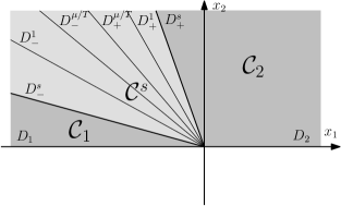
Figure 1: The cones ${\cal{C}}_{1}$, ${\cal{C}}^{s}$, ${\cal{C}}_{2}$.

A key step in the proof of Theorem 11 is to evaluate for how much time a trajectory of (19) stays in each of the three cones.

Lemma 13

There exists a positive constant $C_{1}=C_{1}(\rho,T,\mu)$ (i.e., only depending on $\rho$, $T$, and $\mu$) such that, for every $\lambda\geq k$, every $(T/\lambda,\mu/\lambda)$-signal $\alpha$, every $x_{*}\in\mathbb{R}^{2}\setminus\{0\}$, and every $t_{0}\geq 0$, if an interval $I\subset\mathbb{R}$ is such that the trajectory $t\mapsto x(t;t_{0},x_{*},K,\alpha)$ stays in ${\cal{C}}_{1}\cup{\cal{C}}_{2}$ for every $t\in I$ then the length of $I$ is smaller than $C_{1}/k$.

Proof of Lemma 13. Consider $\alpha\in L^{\infty}(\mathbb{R}_{\geq 0},[0,1])$ and a trajectory $x(\cdot):=x(\cdot\,;t_{0},x_{*},K,\alpha)$ of (19) with $x_{*}\in\mathbb{R}^{2}\setminus\{0\}$ and $t_{0}\geq 0$. Let $I=[t_{1},t_{2}]$ be a time-interval such that $x(t)$ belongs to ${\cal{C}}_{1}\cup{\cal{C}}_{2}$ for every $t\in I$.

Using polar coordinates, $x(\cdot)$ can be represented as $t\mapsto(r(t)\cos\theta(t),r(t)\sin\theta(t))$ and one has

$$\dot{\theta}=\frac{\dot{x}_{1}\sin\theta-\dot{x}_{2}\cos\theta}{r}=-\sin^{2}\theta+\alpha\cos\theta\left(\frac{\rho k^{2}}{2}\cos\theta+k\sin\theta\right)$$

almost everywhere in $I$. Therefore,

$$\dot{\theta}\leq-\alpha\left(\sin^{2}\theta+k\cos\theta\sin\theta+\frac{\rho k^{2}}{2}\cos^{2}\theta\right).$$

We next show that there exists a positive constant $c(\rho)$ such that

$$\dot{\theta}\leq-\alpha c(\rho)(\sin^{2}\theta+k^{2}\cos^{2}\theta),$$ (25)

almost everywhere in $I$. The claim can be proved by taking $\tau:=\tan(\theta)$ and noticing that there exists $c(\rho)>0$ small enough such that if $\tau<\xi^{s}_{+}$ or $\tau>\xi^{s}_{-}$ then

$$\tau^{2}+k\tau+\frac{\rho k^{2}}{2}\geq c(\rho)(\tau^{2}+k^{2}).$$

Define now

$$F(\theta)=\left\{\begin{array}[]{ll}\arctan\left(\frac{\tan\theta}{k}\right)&\mbox{if }0\leq\theta<\pi/2,\\ \pi/2&\mbox{if }\theta=\pi/2,\\ \arctan\left(\frac{\tan\theta}{k}\right)+\pi&\mbox{if }\pi/2<\theta\leq\pi.\end{array}\right.$$

Notice that $F$ is a continuous reparameterization of the interval $[0,\pi]$. From (25), we get

$$\frac{d}{dt}(F(\theta))\leq-c(\rho)k\alpha.$$ (26)

Therefore, $F(\theta)$ is monotone non-increasing as long as $x(\cdot)$ stays in ${\cal{C}}_{1}\cup{\cal{C}}_{2}$. If $\alpha$ is a $(T/\lambda,\mu/\lambda)$-signal, then

$$F\left(\theta\left(t+\frac{T}{\lambda}\right)\right)-F(\theta(t))\leq-\frac{c(\rho)\mu k}{\lambda}$$ (27)

for every $t$ with $[t,t+T/\lambda]\subset I$. Let $l^{\max}$ be the largest integer such that $I$ contains $l^{\max}$ disjoint sub-intervals of length $T/\lambda$. Then (27) yields

$$\pi\geq F(\theta(t_{1}))-F(\theta(t_{2}))\geq l^{\max}\frac{c(\rho)\mu k}{\lambda}$$

and thus

$$l^{\max}\leq\frac{\lambda\pi}{c(\rho)\mu k}.$$

Hence

$$t_{2}-t_{1}\leq(l^{\max}+1)\frac{T}{\lambda}\leq\frac{T\pi}{c(\rho)\mu k}+\frac{T}{\lambda}.$$

The lemma is concluded by recalling the hypothesis $\lambda\geq k$.    

From now until the end of the proof, let $x_{0}\neq 0$ belong to the cone defined by $D_{1}$ and $D^{s}_{+}$, i.e., to ${\cal{C}}_{1}\cup{\cal{C}}^{s}$. Let, moreover, $t_{0}\geq 0$, $\lambda\geq k$, $\alpha\in{\cal G}(T/\lambda,\mu/\lambda)$, and define $x(\cdot):=x(\cdot\,;t_{0},x_{0},K,\alpha)$. Then the following alternative occurs for $x(\cdot)$:

$(i)$

for every $t\geq t_{0}$, $x(t)$ remains in ${\cal{C}}_{1}\cup{\cal{C}}^{s}$;

$(ii)$

$x(\cdot)$ reaches $D^{s}_{+}$ in finite time.

In both cases, let $[t_{0},t_{1}]$ be the time-interval needed by $x(\cdot)$ to reach ${\cal C}^{s}$. Recall that, by Lemma 13, one has $0\leq t_{1}-t_{0}<C_{1}/k$. We notice the following fact, which results from a trivial computation.

Lemma 14

The positive definite function $V(x):=x_{1}^{2}+2x_{2}^{2}/\rho k^{2}$, evaluated along $x(\cdot)$, is non-increasing as long as $x(\cdot)$ remains in the fourth quadrant, i.e. $\{x\in\mathbb{R}^{2}:x_{1}\leq 0,x_{2}\geq 0\}$.

The following lemma provides an exponential decay result for trajectories staying in ${\cal C}^{s}$ (in particular, for trajectories satisfying ($i$)).

Lemma 15

There exist $C_{2}=C_{2}({\color[rgb]{0,0,0}\rho,k},T,\mu)>0$ and $\gamma=\gamma(\rho,T,\mu)>0$ such that, for every $t\geq t_{1}$ such that $x(\cdot)$ stays in ${\cal C}^{s}$ along the interval $[t_{1},t]$, it holds that

$$|x(t)|\leq C_{2}e^{-k\gamma(t-t_{1})}|x_{0}|.$$ (28)

Moreover, $C_{2}=O(k)$ as a function of $k$ as $k$ tends to infinity.

Proof of Lemma 15. Let $t$ be as in the statement of the lemma. We deduce that, for $\tau\in(t_{1},t)$,

$$\dot{x}_{2}(\tau)=-k\alpha(\tau)w(\tau)x_{2}(\tau),$$

where $w(\cdot)$ is a continuous function verifying

$$0<1+\frac{\rho k}{2\xi^{s}_{-}}\leq w(\tau)\leq 1+\frac{\rho k}{2\xi^{s}_{+}}.$$

Notice that the bounds on $w$ do not depend on $k$, due to the definition of $\xi^{s}_{\pm}$. We are back to the (PE) one-dimensional case studied in the introduction. We deduce that there exist $C_{*}=C_{*}(\rho,T,\mu)>0$ and $\gamma=\gamma(\rho,T,\mu)>0$ such that

$$x_{2}(t)\leq C_{*}e^{-k\gamma(t-t_{1})}x_{2}(t_{1}).$$ (29)

Notice now that, for every $x\in{\cal C}^{s}$,

$$|x|\leq x_{2}\sqrt{1+\frac{1}{(\xi_{+}^{s})^{2}}},\ \ \ \ \ \ x_{2}\leq k\sqrt{\frac{\rho}{2}}\sqrt{V(x)},\ \ \ \ \ \ \sqrt{V(x)}\leq\max\left\{1,{\color[rgb]{0,0,0}\frac{1}{k}\sqrt{\frac{2}{\rho}}}\right\}|x|.$$

The proof of the lemma is concluded by recalling that $V(x(t_{1}))\leq V(x_{0})$ and plugging the above estimates in (29).    

Let us now establish a lower bound on the time needed to go across the cone ${\cal C}^{s}$.

Lemma 16

There exists $\lambda_{0}>0$ such that if $\lambda\geq\lambda_{0}$ and $x_{0}\in D^{s}_{-}$ then $x(\cdot)$ stays in ${\cal C}^{s}$ for all $t\in[t_{0},t_{0}+1]$.

Proof of Lemma 16. Fix $x_{0}\in D^{s}_{-}$. Reasoning by contradiction (and exploiting the homogeneity of (19)) we assume that there exist a strictly increasing unbounded sequence $\{\lambda_{i}\}_{i\in\mathbb{N}}$ and a sequence $\{\alpha_{i}\}_{i\in\mathbb{N}}\subset L^{\infty}(\mathbb{R}_{\geq 0},[0,1])$ with $\alpha_{i}\in{\cal{G}}(T/\lambda_{i},\mu/\lambda_{i})$ such that each $x_{i}(\cdot):=x(\cdot\,;t_{0},x_{0},K,\alpha_{i})$, $i\in\mathbb{N}$, reaches $D^{s}_{+}$ in time smaller than one. Because of the sequential weak-$\star$ compactness of $L^{\infty}(\mathbb{R}_{\geq 0},[0,1])$, there exists $\alpha_{\star}\in L^{\infty}(\mathbb{R}_{\geq 0},[0,1])$ and a subsequence of $\{\lambda_{i}\}_{i\in\mathbb{N}}$ (still denoted by $\{\lambda_{i}\}_{i\in\mathbb{N}}$) such that $\{\alpha_{i}\}_{i\in\mathbb{N}}$ converges weakly-$\star$ to $\alpha_{\star}$.

By Proposition 21, we deduce that the sequence $\{x_{i}\}_{i\in\mathbb{N}}$ converges, uniformly on compact time-intervals, and in particular on $[t_{0},t_{0}+1]$, to $x_{\star}(\cdot):=x(\cdot\,;t_{0},x_{0},K,\alpha_{\star})$. Since, for every $i\in\mathbb{N}$, $x_{i}(\cdot)$ reaches $D^{s}_{+}$ in time smaller than one, we deduce that $x_{\star}(t_{0}+t_{\star})\in D^{s}_{+}$ for some $t_{\star}\in(0,1]$.

Let us show that $\alpha_{\star}\geq\mu/T$ almost everywhere on $\mathbb{R}_{\geq 0}$. For every interval $J\subset\mathbb{R}_{\geq 0}$ of finite length $\ell>0$, apply (15) to the characteristic function of $J$. Since each $\alpha_{\lambda_{i}}$ is a $(T/{\lambda_{i}},\mu/{\lambda_{i}})$-signal, it follows that

$$\frac{1}{\ell}\int_{J}\alpha_{\star}(s)ds=\lim_{i\to\infty}\frac{1}{\ell}\int_{J}\alpha_{i}(s)ds\geq\liminf_{i\to\infty}\frac{\mu}{\ell\lambda_{i}}{\cal I}\left(\frac{\ell\lambda_{i}}{T}\right)=\frac{\mu}{T}\,,$$

where ${\cal I}(\cdot)$ denotes the integer part. Recall that since $\alpha_{\star}$ is measurable and bounded (actually, $L^{1}$ would be enough), almost every $t>0$ is a Lebesgue point for $\alpha_{\star}$, i.e., the limit

$$\lim_{\varepsilon\to 0+}\frac{1}{2\varepsilon}\int_{t-\varepsilon}^{t+\varepsilon}\alpha_{\star}(s)ds$$

exists and is equal to $\alpha_{\star}(t)$ (see, for instance, [11]). We conclude that, as claimed, $\alpha_{\star}(t)\geq\mu/T$ almost everywhere.

Therefore, $x_{\star}(\cdot)$ is actually a trajectory of the switching system

$$\dot{x}=\left[u(A+bK^{\top})+(1-u)\left(A+\frac{\mu}{T}bK^{\top}\right)\right]x,$$ (30)

where $u$ is a measurable function defined on $\mathbb{R}_{\geq 0}$ and taking values in $[0,1]$ (see [1] and references therein for more on switching systems). According to the taxonomy and the results in [1, page 93], (30) is a switching system of type $(RR.2.2.A)$ and, as a consequence, the curve $x_{\star}$ stays below the trajectory $\bar{x}$ of (30) starting from $x_{0}$ at time $t_{0}$ and corresponding to the input $u\equiv 0$. Since $\bar{x}$ converges to zero in the cone delimited by $D^{s}_{-}$ and $D^{\mu/T}_{-}$, $x_{\star}$ must stay in the same cone, contradicting the fact that $x_{\star}$ reaches $D^{s}_{+}$ in finite time. Lemma 16 is proved.    

Let us now focus on the behavior of trajectories exiting ${\cal C}^{s}$ or, equivalently, such that $x_{0}\in D^{s}_{+}$.

Lemma 17

There exists $\lambda_{1}\geq k$ such that if $\lambda\geq\lambda_{1}$ and $x_{0}\in D^{s}_{+}$ then there exists a finite time $t_{f}>0$ such that $x(\cdot)$ satisfies

$$|x(t_{f})|\leq|x_{0}|,$$ (31)

with $x(t_{f})\in D_{2}$ and $x(t)\in{\cal C}_{2}$ for all $t\in[t_{0},t_{f}]$.

Proof of Lemma 17. Fix $x_{0}\in D^{s}_{+}$. We reason again by contradiction and follow the same procedure as in Lemma 16. This is possible since, according to Lemma 15, the time needed by any trajectory of (19) to go across in ${\cal{C}}_{2}$ is bounded (uniformly with respect to $\lambda\geq k$ and $\alpha\in{\cal{G}}(T/\lambda,\mu/\lambda)$) by $C_{1}/k$. We obtain that, for some $t_{0}<t^{\prime}_{f}\leq C_{1}/k$, the limit trajectory $x_{\star}$ is contained in ${\cal C}_{2}$ on $[t_{0},t_{f}^{\prime}]$, reaches $D_{2}$ at time $t_{f}^{\prime}$, and satisfies $|x_{\star}(t^{\prime}_{f})|\geq|x_{0}|$. According to [1], the trajectory $x_{\star}$ is, inside ${\cal{C}}_{2}$, below the integral curve $x_{\mu/T}$ of $\dot{x}=(A+\frac{\mu}{T}bK^{\top})x$ with initial condition $x_{\mu/T}(t_{0})=x_{0}$. That means in particular that $|x_{\star}(t^{\prime}_{f})|\leq|x_{\mu/T}(t^{\prime\prime}_{f})|$, where $t^{\prime\prime}_{f}$ is the first time larger than $t_{0}$ such that $x_{\mu/T}(t^{\prime\prime}_{f})\in D_{2}$. However, a lengthy but straightforward computation shows that $|x_{\mu/T}(t^{\prime\prime}_{f})|<|x_{0}|$ and we reach a contradiction.    

Define $\lambda_{*}=\max\{\lambda_{0},\lambda_{1}\}$ where $\lambda_{0}$ and $\lambda_{1}$ are the quantities appearing in the statements of Lemmas 16 and 17. Whenever $x(\cdot)$ satisfies ($ii$) we let $(t_{1}\leq)t_{2}<t_{f}$ be such that $x(t)\in{\cal C}^{s}$ for $t\in[t_{1},t_{2}]$, $x(t)\in{\cal C}_{2}$ for $t\in[t_{2},t_{f}]$, and $x(t_{f})\in D_{2}$.

As a final technical result for the completion of the argument, we need the following lemma.

Lemma 18

There exist $k_{*}=k_{*}(\rho,T,\mu)>0$ and $\gamma_{*}=\gamma_{*}(\rho,T,\mu)>0$ such that if $x(\cdot)$ satisfies $(ii)$, $t_{f}-t_{0}\geq 1$, $k\geq k_{*}$, and $\lambda\geq\lambda_{*}$, then

$$|x(t_{f})|\leq\frac{1}{2}e^{-k\gamma_{*}(t_{f}-t_{0})}|x_{0}|.$$ (32)

Proof of Lemma 18. Applying estimates (28) and (31) we get that

$$|x(t_{f})|\leq|x(t_{2})|\leq C_{2}e^{-k\gamma(t_{2}-t_{1})}|x_{0}|\,.$$

Moreover, according to Lemma 13 and the hypothesis $t_{f}-t_{0}\geq 1$,

$$|x(t_{f})|\leq C_{2}e^{2\gamma C_{1}}e^{-k\gamma(t_{f}-t_{0})}|x_{0}|\leq C_{2}e^{2\gamma C_{1}-k\gamma/2}e^{-k\gamma(t_{f}-t_{0})/2}|x_{0}|\,.$$

The lemma is proved by taking $\gamma_{*}=\gamma/2$ and $k_{*}$ large enough in order to have $C_{2}e^{2\gamma C_{1}-k\gamma/2}\leq 1/2$. Such a $k_{*}$ does exist because, in view of Lemmas 13 and 15, neither $C_{1}$ nor $\gamma$ depend on $k$, while $C_{2}=O(k)$ as $k$ tends to infinity.    

We have developed enough tools to conclude the proof of Theorem 11. Take $k\geq k_{*}$ and $\lambda\geq\lambda_{*}$. Let $\xi_{0}\in\mathbb{R}^{2}\setminus\{0\}$, $t_{0}\geq 0$, $\alpha\in{\cal G}(T/\lambda,\mu/\lambda)$, and denote by ${\cal T}$ the set of times such that $\xi(\cdot)=x(\cdot\,;t_{0},\xi_{0},\alpha)$ belongs to the $x_{1}$-axis. Choose one representative for every connected component of ${\cal T}$. Denote by ${\cal T}^{\prime}$ the set of such representatives and by $j\in\mathbb{N}\cup\{+\infty\}$ its cardinality. By monotonically enumerating the elements of ${\cal T}^{\prime}$, we have ${\cal T}^{\prime}=\{\tau_{i}\mid 0\leq i<j\}$ with $\tau_{i-1}<\tau_{i}$ for $0<i<j$. Let, moreover, $\tau_{-1}=t_{0}$ and $\tau_{j}=+\infty$. Since, for every $-1\leq i<j$, either $\xi(\cdot)$ or $-\xi(\cdot)$, restricted to $(\tau_{i},\tau_{i+1})$, is contained in the upper half-plane, then the previously established estimates apply to it.

Take $-1\leq i<j$ and $t\in[\tau_{i},\tau_{i+1})$. Then there exists $C_{3}=C_{3}(K,T,\mu)>1$ such that

$$|\xi(t)|\leq C_{3}e^{-k\gamma_{*}(t-\tau_{i})}|\xi(\tau_{i})|.$$ (33)

Indeed, let

$$s_{1} = \sup\{s\in[\tau_{i},t]\mid\xi([\tau_{i},s])\subset{\cal C}_{1}\mbox{ or }-\xi([\tau_{i},s])\subset{\cal C}_{1}\},$$

$$s_{2} = \inf\{s\in[\tau_{i},t]\mid\xi([s,t])\subset{\cal C}_{2}\mbox{ or }-\xi([s,t])\subset{\cal C}_{2}\},$$

and notice that $\max\{s_{1}-\tau_{i},t-s_{2}\}<C_{1}/k$. Then (33) immediately follows from Lemma 15.

In particular, if $j>0$ then

$$|\xi(\tau_{0})|\leq C_{3}e^{-k\gamma_{*}(\tau_{0}-t_{0})}|\xi_{0}|.$$

Moreover, for every $0<i<j$, Lemma 18 yields

$$|\xi(\tau_{i})|\leq\frac{1}{2}e^{-k\gamma_{*}(\tau_{i}-\tau_{i-1})}|\xi(\tau_{i-1})|,$$

which implies, by recurrence, that

$$|\xi(\tau_{i})|\leq\frac{1}{2}e^{-k\gamma_{*}(\tau_{i}-\tau_{0})}|\xi(\tau_{0})|.$$

Therefore, independently of $j$, for every $-1\leq i<j$ we have

$$|\xi(\tau_{i})|\leq C_{3}e^{-k\gamma_{*}(\tau_{i}-t_{0})}|\xi_{0}|.$$

Applying again (33) we obtain that for every $t\in[t_{0},+\infty)=\bigcup_{i=1}^{j-1}[\tau_{i-1},\tau_{i})$,

$$|\xi(t)|\leq C_{3}^{2}e^{-k\gamma_{*}(t-t_{0})}|\xi_{0}|\,,$$

which proves Theorem 11.    

Let us go back to the natural question posed in $(Q1)$, that is, whether the choice of a stabilizer $K$ can be made independently of $T$ and $\mu$. Unlike the case when $A$ is neutrally stable, we prove below that the answer is negative when the double integrator is considered.

Proposition 19

For every $K\in\mathbb{R}^{2}$, there exist $T\geq\mu>0$ such that $K$ is not a $(T,\mu)$-stabilizer for system (18).

Proof of Proposition 19. Let $K=(-k_{1},-k_{2})\in\mathbb{R}^{2}$. If $k_{1}\leq 0$ or $k_{2}\leq 0$ then $A+bK$ is not Hurwitz and thus $K$ is not a $(T,\mu)$-stabilizer for system (18), whatever $\mu$ and $T$. Let now $k_{1},k_{2}>0$. Among the possible configurations of the right-hand side of (19), we focus our attention on the linear vector fields $L_{0}$ and $L_{1}$, corresponding to $\alpha(t)=0$ and to $\alpha(t)=1$ respectively, that is,

$$L_{0}(x):=A\,x\,,\quad L_{1}(x):=\left(\begin{array}[]{cc}0&1\\ -k_{1}&-k_{2}\end{array}\right)x\,.$$

Consider the set where $L_{0}$ and $L_{1}$ are collinear, i.e., the union of the axis $\{x_{2}=0\}$ and the line $D$ defined by

$$D:=\{(x_{1},x_{2})\in\mathbb{R}^{2}\mid x_{2}=-(k_{1}/k_{2})x_{1}\}\,.$$

We denote by $Q_{1},Q_{2},Q_{3},$ and $Q_{4}$ the four regions of the plane delimited by these two lines and defined as follows

$$Q_{1} := \{(x_{1},x_{2})\in\mathbb{R}^{2}\mid x_{2}\geq-(k_{1}/k_{2})x_{1}\,,x_{2}>0\},$$

$$Q_{2} := \{(x_{1},x_{2})\in\mathbb{R}^{2}\mid x_{2}>-(k_{1}/k_{2})x_{1}\,,x_{2}\leq 0\},$$

$$Q_{3} := \{(x_{1},x_{2})\in\mathbb{R}^{2}\mid x_{2}\leq-(k_{1}/k_{2})x_{1}\,,x_{2}<0\},$$

$$Q_{4} := \{(x_{1},x_{2})\in\mathbb{R}^{2}\mid x_{2}<-(k_{1}/k_{2})x_{1}\,,x_{2}\geq 0\}.$$

Roughly speaking, on $Q_{2}\cup Q_{4}$ the vector field $L_{1}$ points “more outwards” than $L_{0}$ (with respect to the origin). Therefore, on $Q_{2}\cup Q_{4}$ the excitation ($\alpha=1$) is not helping the stability towards the origin (see Figure 2).

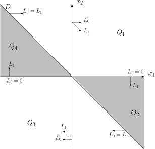
Figure 2: Partition of the state-space into the four regions $Q_{1},Q_{2},Q_{3},Q_{4}$.

We look for a “destabilizing” $\alpha$ in the form $\zeta(x(\cdot))$, where $x(\cdot)$ is an unbounded solution corresponding to the feedback

$$\zeta(x)=\left\{\begin{array}[]{ll}1&\mbox{if }x\in Q_{2}\cup Q_{4},\\ \mu/T&\mbox{if }x\in Q_{1}\cup Q_{3},\end{array}\right.$$

$\mu$ and $T$ to be chosen. Clearly, any $\alpha$ obtained in such a way is a $(T,\mu)$-signal. (It should be stressed that although $\zeta$ is a discontinuous feedback, its solutions are anyway well-defined because all trajectories of (18) are rotating around the origin).

Let $\bar{x}$ be the first intersection with $D$ of the trajectory of (19) starting from $(-1,0)$ and corresponding to $\alpha\equiv 1$. Notice that there exists $\nu>0$ small enough such that the trajectory of (19) starting from $\bar{x}$ and corresponding to $\alpha\equiv\nu$ crosses the $x_{1}$-axis at a point $(\xi,0)$ such that $\xi>1$. This is because as $\nu\to 0$ such trajectories converge uniformly on compact intervals to the horizontal curve $t\mapsto e^{tA}\bar{x}$.

Fix $T\geq\mu>0$ such that $\mu/T\geq\nu$. Then the trajectory $x(\cdot)$ of (19) starting from $(-1,0)$ and corresponding to the feedback $\zeta$ first leaves the upper half-plane through $[\xi,+\infty)\times\{0\}$. Then, by symmetry and homogeneity of the system, $|x(t)|$ goes to infinity as $t\to\infty$. Thus, $\alpha(t)=\zeta(x(t))$ is the required destabilizing signal.    

4.2 Non-scalar control

It makes sense to consider the stability properties of the system whose linear dynamics is the same as that of the double integrator, but which has a different controlled part. That is, we study system

$$\dot{x}=\left(\begin{array}[]{cc}0&1\\ 0&0\end{array}\right)x+\alpha Bu,\ \ \ \ \ x\in\mathbb{R}^{2},\ \ \ \ \ u\in\mathbb{R}^{m},$$ (34)

where $B$ is a general $2\times m$ matrix such that the pair $(A,B)$ is controllable ($A$ denotes the nilpotent $2\times 2$ matrix appearing in (34)). Since the image of $A$ is one-dimensional, the controllability of $(A,B)$ implies the existence of a column $b$ of $B$ such that $(A,b)$ is controllable. Moreover, by a linear change of coordinates, we can transform $(A,b)$ into its Brunovsky normal form, that is, into the matrix $A$ and the vector $b=(0,1)^{\top}$ as in (17). Therefore Theorem 11 guarantees that for every pair of positive constants $\mu\leq T$ there exists a $(T,\mu)$-stabilizer for (4).

The difference with respect to the scalar case is that Proposition 19 is not valid anymore when the rank of $B$ equals two, that is, the answer to question $(Q1)$ becomes positive.

Proposition 20

If $\mathrm{rank}(B)=2$, then there exists $K$ of size $m\times 2$ such that for every $T\geq\mu>0$ the gain $K$ is a $(T,\mu)$-stabilizer for system (34).

Proof of Proposition 19. Let us remark that, up to a reparameterization of $\mathbb{R}^{m}$ of the type $u^{\prime}=Mu$, $M$ invertible, we can rewrite $B$ as $(\mathrm{Id}\ {\bf 0})$, where $\mathrm{Id}$ is the $2\times 2$ identity matrix and all the entries of the $2\times(m-2)$ matrix ${\bf 0}$ are null. That is, (34) is equivalent to

$$\dot{x}=Ax+\alpha u,\ \ \ \ \ x\in\mathbb{R}^{2},\ \ \ \ \ u\in\mathbb{R}^{2}.$$ (35)

Fix $k>0$ and take $u=-kx$. If $t\mapsto x(t)$ is a solution of

$$\dot{x}=(A-\alpha k\mathrm{Id})x,$$

then $t\mapsto y(t):=e^{-At}x(t)$ satisfies $\dot{y}=-k\alpha y$. Therefore

$$y(t)=\exp\left(-k\int_{0}^{t}\alpha(\tau)d\tau\right)y(0)\,,$$

which implies that

$$\left|{x(t)}\right|\leq\left|{e^{At}}\right|\exp\left(-k\int_{0}^{t}\alpha(\tau)d\tau\right)\left|{x(0)}\right|.$$

Since $e^{At}=\mathrm{Id}+tA$ is linear in $t$, we have proved that for every $T\geq\mu>0$ and for every $k>0$ the gain $K=-k\mathrm{Id}$ is a $(T,\mu)$-stabilizer for system (35).    

5 Appendix

We first provide a simple result used several times in the paper.

Proposition 21

Consider system (9), where $A,B,K$ are matrices of size $n\times n$, $n\times m$ and $m\times n$ respectively, and $\alpha$ is a $(T,\mu)$-signal. Take a sequence $x_{0i}$ of norm-one vectors converging to $x_{0*}$ and a bounded sequence $\alpha_{i}$ in $L^{\infty}({\mathbb{R}})$ which converges weakly-$\star$ (in $L^{\infty}({\mathbb{R}})$) to a measurable function $\alpha_{\star}$. Then the sequence $\{x_{i}(\cdot):=x(\cdot,0,x_{0i},K,\alpha_{i})\}_{i\in\mathbb{N}}$ converges, uniformly on compact time intervals, to $x_{\star}(\cdot):=x(\cdot,0,x_{0\star},K,\alpha_{\star})$ as $i$ tends to infinity.

Proof of Proposition 21. Recall that the weakly-$\star$ convergence of $\alpha_{i}$ to $\alpha_{\star}$ means that, for every $\varphi\in L^{1}(\mathbb{R}_{\geq 0},\mathbb{R})$, it holds that

$$\lim_{i\to\infty}\int_{0}^{\infty}\alpha_{i}(s)\varphi(s)ds=\int_{0}^{\infty}\alpha_{\star}(s)\varphi(s)ds\,.$$

Taking as $\varphi$ the characteristic function of an arbitrary interval of length $T$ shows that $\alpha_{\star}$ is a $(T,\mu)$-signal. Moreover, the norm of $x_{0*}$ is equal to one. For $i\in\mathbb{N}$, set

$$e_{i}(\cdot)=x_{i}(\cdot)-x_{\star}(\cdot),\ \ e_{0i}=x_{0i}-x_{0*},$$

$$A_{i}(\cdot)=A+\alpha_{i}(\cdot)BK,$$

and let $\phi_{i}(\cdot,\cdot)$ be the fundamental solution of $\dot{x}=A_{i}(t)x$. Integrating the differential equation verified by $e_{i}$, one gets, for $t\geq 0$,

$$e_{i}(t)=\int_{0}^{t}A_{i}(s)e_{i}(s)ds+h_{i}(t),$$

where $h_{i}(t)=\phi_{i}(t,0)e_{0i}+\int_{0}^{t}(\alpha_{i}(s)-\alpha_{\star}(s))BKx_{\star}(s)ds$. Note that the functions $h_{i}$ are uniformly bounded over compact time-intervals and the sequence they define converges point-wise to zero as $i$ tends to infinity. Therefore, by combining Gronwall Lemma and the bounded convergence theorem, it follows that the sequence $\{e_{i}(\cdot)\}_{i\in\mathbb{N}}$ converges point-wise to zero as $i$ tends to infinity. The uniform convergence on compact time intervals results from the above combined with Ascoli theorem.

References

- [1] U. Boscain, “Stability of planar switched systems: the linear single input case”, SIAM J. Control Optim., vol. 41, pp. 89–112, 2002.
- [2] M. S. Branicky, “Multiple Lyapunov functions and other analysis tools for switched and hybrid systems”, IEEE Trans. Automat. Control, vol. 43, pp. 475–482, 1998.
- [3] H. Brezis, Analyse fonctionnelle, Théorie et applications. Collection Mathématiques Appliquées pour la Maîtrise, Masson, 1983.
- [4] P. Colaneri, J. C. Geromel, and A. Astolfi, “Stabilization of continuous-time nonlinear switched systems”, in Proc. 44th IEEE Conf. Decision Contr., (Sevilla, Spain), December 2005.
- [5] I. I. Gihman, “Concerning a theorem of N. N. Bogolyubov” (Russian), Ukrain. Mat. Ž., vol. 4, pp. 215–219, 1952.
- [6] J. P. Hespanha, D. Liberzon, D. Angeli, and E. D. Sontag, “Nonlinear norm-observability notions and stability of switched systems”, IEEE Trans. Automat. Control, vol. 50, pp. 154–168, 2005.
- [7] D. Liberzon, Switching in Systems and Control. Systems and Control: Foundations and Applications, Boston, MA, Birkhäuser, 2003.
- [8] W. Liu and H. J. Sussmann, “Continuous dependence with respect to the input of trajectories of control-affine systems”, SIAM J. Control Optim., vol. 37, pp. 777–803, 1999.
- [9] A. Loría, A. Chaillet, G. Besancon, and Y. Chitour, “On the PE stabilization of time-varying systems: open questions and preliminary answers”, in Proc. 44th IEEE Conf. Decision Contr., (Sevilla, Spain), pp. 6847–6852, December 2005.
- [10] A. P. Morgan and K. S. Narendra, “On the stability of nonautonomous differential equations with skew-symmetric matrix ”, SIAM J. Control Optim., vol. 15, pp. 163–176, 1977.
- [11] I. E. Segal and R. A. Kunze, Integrals and operators. Berlin-New York: Springer-Verlag, 1978.
- [12] R. Shorten, F. Wirth, O. Mason, K. Wulff, and C. King, “Stability criteria for switched and hybrid systems”, to appear in SIAM Review, 2007.
- [13] E. Sontag, Mathematical Control Theory: Deterministic Finite Dimensional Systems. New York: Springer-Verlag, 1998.
- [14] A. R. Teel, J. Peuteman, and D. Aeyels, Semi-global practical stability and averaging, Systems and Control Letters, vol. 37, pp. 329–334, 1999.