A randomized Kaczmarz algorithm with exponential convergence

Abstract

The Kaczmarz method for solving linear systems of equations is an iterative algorithm that has found many applications ranging from computer tomography to digital signal processing. Despite the popularity of this method, useful theoretical estimates for its rate of convergence are still scarce. We introduce a randomized version of the Kaczmarz method for consistent, overdetermined linear systems and we prove that it converges with expected exponential rate. Furthermore, this is the first solver whose rate does not depend on the number of equations in the system. The solver does not even need to know the whole system, but only a small random part of it. It thus outperforms all previously known methods on general extremely overdetermined systems. Even for moderately overdetermined systems, numerical simulations as well as theoretical analysis reveal that our algorithm can converge faster than the celebrated conjugate gradient algorithm. Furthermore, our theory and numerical simulations confirm a prediction of Feichtinger et al. in the context of reconstructing bandlimited functions from nonuniform sampling.

1 Introduction and state of the art

We study a consistent linear system of equations

$$Ax=b,$$ (1)

where $A$ is a full rank $m\times n$ matrix with $m\geq n$, and $b\in\mathbb{C}^{m}$. One of the most popular solvers for such overdetermined systems is Kaczmarz’s method [28], which is a form of alternating projection method. This method is also known under the name Algebraic Reconstruction Technique (ART) in computer tomography [24, 30], and in fact, it was implemented in the very first medical scanner [27]. It can also be considered as a special case of the POCS (Projection onto Convex Sets) method, which is a prominent tool in signal and image processing [34, 4].

We denote the rows of $A$ by $a_{1}^{\ast},\dots,a_{m}^{\ast}$ and let $b=(b_{1},\dots,b_{m})^{T}$. The classical scheme of Kaczmarz’s method sweeps through the rows of $A$ in a cyclic manner, projecting in each substep the last iterate orthogonally onto the solution hyperplane of $\langle a_{i},x\rangle=b_{i}$ and taking this as the next iterate. Given some initial approximation $x_{0}$, the algorithm takes the form

$$x_{k+1}=x_{k}+\frac{b_{i}-\langle a_{i},x_{k}\rangle}{\|a_{i}\|_{2}^{2}}a_{i},$$ (2)

where $i=k\mod m+1$ and $\|\cdot\|$ denotes the Euclidean norm in $\mathbb{C}^{n}$. Note that we refer to one projection as one iteration, thus one sweep in (2) through all $m$ rows of $A$ consists of $m$ iterations.

While conditions for convergence of this method are readily established, useful theoretical estimates of the rate of convergence of the Kaczmarz method (or more generally of the alternating projection method for linear subspaces) are difficult to obtain, at least for $m>2$. Known estimates for the rate of convergence are based on quantities of the matrix $A$ that are hard to compute and difficult to compare with convergence estimates of other iterative methods (see e.g. [7, 8, 15] and the references therein).

What numerical analysts would like to have is estimates of the convergence rate in terms of a condition number of $A$. No such estimates have been known prior to this work. The difficulty stems from the fact that the rate of convergence of (2) depends strongly on the order of the equations in (1), while condition numbers do not depend on the order of the rows of a matrix.

It has been observed several times in the literature that using the rows of $A$ in Kaczmarz’s method in random order, rather than in their given order, can greatly improve the rate of convergence, see e.g. [30, 4, 26]. While this randomized Kaczmarz method is thus quite appealing for applications, no guarantees of its rate of convergence have been known.

In this paper, we propose the first randomized Kaczmarz method with exponential expected rate of convergence, cf. Section 2. Furthermore, this rate depends only on the scaled condition number of $A$ and not on the number of equations $m$ in the system. The solver does not even need to know the whole system, but only a small random part of it. Thus our solver outperforms all previously known methods on general extremely overdetermined systems.

We analyze the optimality of the proposed algorithm as well as of the derived estimate, cf. Section 3. Section 4 contains various numerical simulations. In one set of experiments we apply the randomized Kaczmarz method to the reconstruction of bandlimited functions from non-uniformly spaced samples. In another set of numerical simulations, accompanied by theoretical analysis, we demonstrate that even for moderately overdetermined systems, the randomized Kaczmarz method can outperform the celebrated conjugate gradient algorithm.

Condition numbers. For a matrix $A$, its spectral norm is denoted by $\|A\|_{2}$, and its Frobenius norm by $\|A\|_{F}$. Thus the spectral norm is the largest singular value of $A$, and the Frobenius norm is the square root of the sum of the squares of all singular values of $A$.

The left inverse of $A$ (which we always assume to exist) is denoted by $A^{-1}$. Thus $\|A^{-1}\|_{2}$ is the smallest constant $M$ such that the inequality $\|Ax\|_{2}\geq\frac{1}{M}\|x\|_{2}$ holds for all vectors $x$.

The usual condition number of $A$ is

$$k(A):=\|A\|_{2}\|A^{-1}\|_{2}.$$

A related version is the scaled condition number introduced by Demmel [6]:

$$\kappa(A):=\|A\|_{F}\|A^{-1}\|_{2}.$$

One easily checks that

$$1\leq\frac{\kappa(A)}{\sqrt{n}}\leq k(A).$$ (3)

Estimates on the condition numbers of some typical (i.e. random or Toeplitz-type ) matrices are known from a big body of literature, see [1, 6, 9, 10, 11, 32, 33, 37, 38] and the references therein.

2 Randomized Kaczmarz algorithm and its rate of convergence

It has been observed in numerical simulations [30, 4, 26] that the convergence rate of the Kaczmarz method can be significantly improved when the algorithm (2) sweeps through the rows of $A$ in a random manner, rather than sequentially in the given order. In fact, the improvement in convergence can be quite dramatic. Here we propose a specific version of this randomized Kaczmarz method, which chooses each row of $A$ with probability proportional to its relevance – more precisely, proportional to the square of its Euclidean norm. This method of sampling from a matrix was proposed in [14] in the context of computing a low-rank approximation of $A$, see also [31] for subsequent work and references. Our algorithm thus takes the following form:

Algorithm 1 (Random Kaczmarz algorithm).

Let $Ax=b$ be a linear system of equations as in (1) and let $x_{0}$ be arbitrary initial approximation to the solution of (1). For $k=0,1,\dots$ compute

$$x_{k+1}=x_{k}+\frac{b_{r(i)}-\langle a_{r(i)},x_{k}\rangle}{\|a_{r(i)}\|_{2}^{2}}a_{r(i)},$$ (4)

where $r(i)$ is chosen from the set $\{1,2,\dots,m\}$ at random, with probability proportional to $\|a_{r(i)}\|_{2}^{2}$.

Our main result states that $x_{k}$ converges exponentially fast to the solution of (1), and the rate of convergence depends only on the scaled condition number $\kappa(A)$.

Theorem 2.

Let $x$ be the solution of (1). Then Algorithm 1 converges to $x$ in expectation, with the average error

$$\mathbb{E}\|x_{k}-x\|_{2}^{2}\leq\bigl{(}1-\kappa(A)^{-2}\bigr{)}^{k}\cdot\|x_{0}-x\|_{2}^{2}.$$ (5)

Proof.   There holds

$$\sum_{j=1}^{m}|\langle z,a_{j}\rangle|^{2}\geq\frac{\|z\|_{2}^{2}}{\|A^{-1}\|_{2}^{2}}\qquad\text{for all $z\in\mathbb{C}^{n}$.}$$ (6)

Using the fact that $\|A\|_{F}^{2}=\sum_{j=1}^{m}\|a_{j}\|_{2}^{2}$ we can write (6) as

$$\sum_{j=1}^{m}\frac{\|a_{j}\|_{2}^{2}}{\|A\|_{F}^{2}}\;\Bigl{|}\Big{\langle}z,\frac{a_{j}}{\|a_{j}\|_{2}}\Big{\rangle}\Big{|}^{2}\geq\kappa(A)^{-2}\|z\|^{2}\ \ \ \text{for all $z\in\mathbb{C}^{n}$}.$$ (7)

The main point of the proof is to view the left hand side in (7) as an expectation of some random variable. Namely, recall that the solution space of the $j$-th equation of (1) is the hyperplane $\{y:\langle y,a_{j}\rangle=b_{j}\}$, whose normal is $\frac{a_{j}}{\|a_{j}\|_{2}}$. Define a random vector $Z$ whose values are the normals to all the equations of (1), with probabilities as in our algorithm:

$$Z=\frac{a_{j}}{\|a_{j}\|_{2}}\ \ \ \text{with probability}\ \ \ \frac{\|a_{j}\|_{2}^{2}}{\|A\|_{F}^{2}},\ \ \ j=1,\ldots,m.$$ (8)

Then (7) says that

$$\mathbb{E}|\langle z,Z\rangle|^{2}\geq\kappa(A)^{-2}\|z\|_{2}^{2}\ \ \ \text{for all $z\in\mathbb{C}^{n}$.}$$ (9)

The orthogonal projection $P$ onto the solution space of a random equation of (1) is given by $Pz=z-\langle z-x,Z\rangle\,Z$.

Now we are ready to analyze our algorithm. We want to show that the error $\|x_{k}-x\|_{2}^{2}$ reduces at each step in average (conditioned on the previous steps) by at least the factor of $(1-\kappa(A)^{-2})$. The next approximation $x_{k}$ is computed from $x_{k-1}$ as $x_{k}=P_{k}x_{k-1}$, where $P_{1},P_{2},\ldots$ are independent realizations of the random projection $P$. The vector $x_{k-1}-x_{k}$ is in the kernel of $P_{k}$. It is orthogonal to the solution space of the equation onto which $P_{k}$ projects, which contains the vector $x_{k}-x$ (recall that $x$ is the solution to all equations). The orthogonality of these two vectors then yields

$$\|x_{k}-x\|_{2}^{2}=\|x_{k-1}-x\|_{2}^{2}-\|x_{k-1}-x_{k}\|_{2}^{2}.$$

To complete the proof, we have to bound $\|x_{k-1}-x_{k}\|_{2}^{2}$ from below. By the definition of $x_{k}$, we have

$$\|x_{k-1}-x_{k}\|_{2}=\langle x_{k-1}-x,Z_{k}\rangle$$

where $Z_{1},Z_{2},\ldots$ are independent realizations of the random vector $Z$. Thus

$$\|x_{k}-x\|_{2}^{2}\leq\Big{(}1-\Big{|}\Big{\langle}\frac{x_{k-1}-x}{\|x_{k-1}-x\|_{2}},Z_{k}\Big{\rangle}\Big{|}^{2}\Big{)}\;\|x_{k-1}-x\|_{2}^{2}.$$

Now we take the expectation of both sides conditional upon the choice of the random vectors $Z_{1},\ldots,Z_{k-1}$ (hence we fix the choice of the random projections $P_{1},\ldots,P_{k-1}$ and thus the random vectors $x_{1},\ldots,x_{k-1}$, and we average over the random vector $Z_{k}$). Then

$$\mathbb{E}_{\{Z_{1},\ldots,Z_{k-1}\}}\|x_{k}-x\|_{2}^{2}\leq\Big{(}1-\mathbb{E}_{\{Z_{1},\ldots,Z_{k-1}\}}\Big{|}\Big{\langle}\frac{x_{k-1}-x}{\|x_{k-1}-x\|_{2}},Z_{k}\Big{\rangle}\Big{|}^{2}\Big{)}\;\|x_{k-1}-x\|_{2}^{2}.$$

By (9) and the independence,

$$\mathbb{E}_{\{Z_{1},\ldots,Z_{k-1}\}}\|x_{k}-x\|_{2}^{2}\leq\big{(}1-\kappa(A)^{-2}\big{)}\;\|x_{k-1}-x\|_{2}^{2}.$$

Taking the full expectation of both sides, we conclude that

$$\mathbb{E}\|x_{k}-x\|_{2}^{2}\leq\big{(}1-\kappa(A)^{-2}\big{)}\;\mathbb{E}\|x_{k-1}-x\|_{2}^{2}.$$

By induction, we complete the proof.  

2.1 Quadratic time

Theorem 2 yields a simple bound on the expected computational complexity of the randomized Kaczmarz Algorithm 1 to compute the solution within error ${\varepsilon}$, i.e.

$$\mathbb{E}\|x_{k}-x\|_{2}^{2}\leq\varepsilon^{2}\|x_{0}-x\|_{2}^{2}.$$ (10)

The expected number of iterations (projections) $k_{\varepsilon}$ to achieve an accuracy ${\varepsilon}$ is

$$\mathbb{E}\,k_{\varepsilon}\leq\frac{2\log\varepsilon}{\log(1-\kappa(A)^{-2})}\approx 2\kappa(A)^{2}\log\frac{1}{\varepsilon},$$ (11)

where $f(n)\sim g(n)$ means $f(n)/g(n)\to 1$ as $n\to\infty$. (Note that $\kappa(A)^{2}\geq n$ by (3), so the approximation in (11) becomes tight as the number of equation $n$ grows).

Since each projection can be computed in $O(n)$ time, and $\kappa(A)^{2}=O(n)$ by (3), the algorithm takes $O(n^{2})$ operations to converge to the solution. This should be compared to the Gaussian elimination, which takes $O(mn^{2})$ time. Strassen’s algorithm and its improvements reduce the exponent in Gaussian elimination, but these algorithms are, as of now, of no practical use.

Of course, we have to know the (approximate) Euclidean lengths of the rows of $A$ before we start iterating; computing them takes $O(nm)$ time. But the lengths of the rows may in many cases be known a priori. For example, all of them may be equal to one (as is the case for Vandermonde matrices arising in trigonometric approximation) or tightly concentrated around a constant value (as is the case for random matrices).

The number $m$ of the equations is essentially irrelevant for our algorithm. The algorithm does not even need to know the whole matrix, but only $O(n)$ random rows. Such Monte-Carlo methods have been successfully developed for many problems, even with precisely the same model of selecting a random submatrix of $A$ (proportional to the squares of the lengths of the rows), see [14] for the original discovery and [31] for subsequent work and references.

3 Optimality

We discuss conditions under which our algorithm is optimal in a certain sense, as well as the optimality of the estimate on the expected rate of convergence.

3.1 General lower estimate

For any system of linear equations, our estimate can not be improved beyond a constant factor, as shown by the following theorem.

Theorem 3.

Consider the linear system of equations (1) and let $x$ be its solution. Then there exists an initial approximation $x_{0}$ such that

$$\mathbb{E}\|x_{k}-x\|_{2}^{2}\geq\big{(}1-2k/\kappa(A)^{2}\big{)}\cdot\|x_{0}-x\|_{2}^{2}$$ (12)

for all $k=1,2,\ldots$

Proof.  For this proof we can assume without loss of generality that the system (1) is homogeneous: $Ax=0$. Let $x_{0}$ be a vector which realizes $\kappa(A)$, that is $\kappa(A)=\|A\|_{F}\|A^{-1}x_{0}\|_{2}$ and $\|x_{0}\|_{2}=1$. As in the proof of Theorem 2, we define the random normal $Z$ associated with the rows of $A$ by (8). Similar to (9), we have $\mathbb{E}|\langle x_{0},Z\rangle|^{2}=\kappa(A)^{-2}$. We thus see ${\rm span}(x_{0})$ as an “exceptional” direction, so we shall decompose $\mathbb{R}^{n}={\rm span}(x_{0})\oplus(x_{0})^{\perp}$, writing every vector $x\in\mathbb{R}^{n}$ as

$$x=x^{\prime}\cdot x_{0}+x^{\prime\prime},\ \ \ \text{where}\ \ \ x^{\prime}\in\mathbb{R},\ \ x^{\prime\prime}\in(x_{0})^{\perp}.$$

In particular,

$$\mathbb{E}|Z^{\prime}|^{2}=\kappa(A)^{-2}.$$ (13)

We shall first analyze the effect of one random projection in our algorithm. To this end, let $x\in\mathbb{R}^{n}$, $\|x\|_{2}\leq 1$, and let $z\in\mathbb{R}^{n}$, $\|z\|_{2}=1$. (Later, $x$ will be the running approximation $x_{k-1}$, and $z$ will be the random normal $Z$). The projection of $x$ onto the hyperplane whose normal is $z$ equals

$$x_{1}=x-\langle x,z\rangle z.$$

Since

$$\langle x,z\rangle=x^{\prime}z^{\prime}+\langle x^{\prime\prime},z^{\prime\prime}\rangle,$$ (14)

we have

$$|x^{\prime}_{1}-x^{\prime}|=|\langle x,z\rangle z^{\prime}|\leq|x^{\prime}||z^{\prime}|^{2}+|\langle x^{\prime\prime},z^{\prime\prime}\rangle z^{\prime}|\leq|z^{\prime}|^{2}+|\langle x^{\prime\prime},z^{\prime\prime}\rangle z^{\prime}|$$ (15)

because $|x^{\prime}|\leq\|x\|_{2}\leq 1$. Next,

$$\|x^{\prime\prime}_{1}\|^{2}-\|x^{\prime\prime}\|^{2} =\|x^{\prime\prime}-\langle x,z\rangle z^{\prime\prime}\|_{2}^{2}-\|x^{\prime\prime}\|_{2}^{2}$$

$$=-2\langle x,z\rangle\langle x^{\prime\prime},z^{\prime\prime}\rangle+\langle x,z\rangle^{2}\|z^{\prime\prime}\|_{2}^{2}\leq-2\langle x,z\rangle\langle x^{\prime\prime},z^{\prime\prime}\rangle+\langle x,z\rangle^{2}$$

because $\|z^{\prime\prime}\|_{2}\leq\|z\|_{2}=1$. Using (14), we decompose $\langle x,z\rangle$ as $a+b$, where $a=x^{\prime}z^{\prime}$ and $b=\langle x^{\prime\prime},z^{\prime\prime}\rangle$ and use the identity $-2(a+b)b+(a+b)^{2}=a^{2}-b^{2}$ to conclude that

$$\|x^{\prime\prime}_{1}\|_{2}^{2}-\|x^{\prime\prime}\|_{2}^{2}\leq|x^{\prime}|^{2}|z^{\prime}|^{2}-\langle x^{\prime\prime},z^{\prime\prime}\rangle^{2}\leq|z^{\prime}|^{2}-\langle x^{\prime\prime},z^{\prime\prime}\rangle^{2}$$ (16)

because $|x^{\prime}|\leq\|x\|_{2}\leq 1$.

Now we apply (15) and (16) to the running approximation $x=x_{k-1}$ and the next approximation $x_{1}=x_{k}$ obtained with a random $z=Z_{k}$. Denoting $p_{k}=\langle x^{\prime\prime}_{k},Z^{\prime\prime}_{k}\rangle$, we have by (15) that $|x^{\prime}_{k}-x^{\prime}_{k-1}|\leq|Z^{\prime}_{k}|^{2}+|p_{k}Z^{\prime}_{k}|$ and by (16) that $\|x^{\prime\prime}_{k}\|_{2}^{2}-\|x^{\prime\prime}_{k-1}\|_{2}^{2}\leq|Z^{\prime}_{k}|^{2}-|p_{k}|^{2}$. Since $x^{\prime}_{0}=1$ and $x^{\prime\prime}_{0}=0$, we have

$$|x^{\prime}_{k}-1|\leq\sum_{j=1}^{k}|x^{\prime}_{j}-x^{\prime}_{j-1}|\leq\sum_{j=1}^{k}|Z^{\prime}_{j}|^{2}+\sum_{j=1}^{k}|p_{j}Z^{\prime}_{j}|$$ (17)

and

$$\|x^{\prime\prime}_{k}\|_{2}^{2}=\sum_{j=1}^{k}\big{(}\|x^{\prime\prime}_{j}\|_{2}^{2}-\|x^{\prime\prime}_{j-1}\|_{2}^{2}\big{)}\leq\sum_{j=1}^{k}|Z^{\prime}_{j}|^{2}-\sum_{j=1}^{k}|p_{j}|^{2}.$$

Since $\|x^{\prime\prime}_{k}\|_{2}^{2}\geq 0$, we conclude that $\sum_{j=1}^{k}|p_{j}|^{2}\leq\sum_{j=1}^{k}|Z^{\prime}_{j}|^{2}$. Using this, we apply Cauchy-Schwartz inequality in (17) to obtain

$$|x^{\prime}_{k}-1|\leq\sum_{j=1}^{k}|Z^{\prime}_{j}|^{2}+\Big{(}\sum_{j=1}^{k}|Z^{\prime}_{j}|^{2}\Big{)}^{1/2}\Big{(}\sum_{j=1}^{k}|Z^{\prime}_{j}|^{2}\Big{)}^{1/2}=2\sum_{j=1}^{k}|Z^{\prime}_{j}|^{2}.$$

Since all $Z_{j}$ are copies of the random vector $Z$, we conclude by (13) that $\mathbb{E}|x^{\prime}_{k}-1|\leq 2k\,\mathbb{E}|Z^{\prime}|^{2}\leq 2k/\kappa(A)^{2}$. Thus $\mathbb{E}\|x_{k}\|\geq\mathbb{E}|x^{\prime}_{k}|\geq 1-2k/\kappa(A)^{2}$. This proves the theorem, actually with the stronger conclusion

$$\mathbb{E}\|x_{k}-x\|_{2}\geq\big{(}1-2k/\kappa(A)^{2}\big{)}\cdot\|x_{0}-x\|_{2}.$$

The actual conclusion follows by Jensen’s inequality.  

3.2 The upper estimate is attained

If $k(A)=1$ (equivalently, if $\kappa(A)=\sqrt{n}$ by (3)), then the estimate in Theorem 2 becomes an equality. This follows directly from the proof of Theorem 2.

Furthermore, there exist arbitrarily large systems and with arbitrarily large condition numbers $k(A)$ for which the estimate in Theorem 2 becomes an equality. Indeed, let $n$ and $m\geq n$ be arbitrary numbers. Let also $\kappa\geq\sqrt{n}$ be any number such that $m/\kappa^{2}$ is an integer. Then there exists a system (1) of $m$ equations in $n$ variables and with $\kappa(A)=\kappa$, for which the estimate in Theorem 2 becomes an equality for every $k$.

To see this, we define the matrix $A$ with the help of any orthogonal set $e_{1},\ldots,e_{n}$ in $\mathbb{R}^{n}$. Let the first $m/\kappa^{2}$ rows of $A$ be equal to $e_{1}$, the other rows of $A$ be equal to one of the vectors $e_{j}$, $j>1$, so that every vector from this set repeats at least $m/\kappa^{2}$ times as a row (this is possible because $\kappa^{2}\geq n$). Then $\kappa(A)=\kappa$ (note that (6) is attained for $z=e_{1}$).

Let us test our algorithm on the system $Ax=0$ with the initial approximation $x_{0}=e_{1}$ to the solution $x=0$. Every step of the algorithm brings the running approximation to $0$ with probability $\kappa^{-2}$ (the probability of picking the row of $A$ equal to $e_{1}$ in uniform sampling), and leaves the running approximation unchanged with probability $1-\kappa^{-2}$. By the independence, for all $k$ we have

$$\mathbb{E}\|x_{k}-x_{0}\|_{2}^{2}=\bigl{(}1-\kappa^{-2}\bigr{)}^{k}\cdot\|x_{0}-x\|_{2}^{2}.$$

4 Numerical experiments and comparisons

4.1 Reconstruction of bandlimited signals from nonuniform sampling

The reconstruction of a bandlimited function $f$ from its nonuniformly spaced sampling values $\{f(t_{k})\}$ is a classical problem in Fourier analysis, with a wide range of applications [2]. We refer to [12, 13] for various efficient numerical algorithms. Staying with the topic of this paper, we focus on the Kaczmarz method, also known as POCS (Projection Onto Convex Sets) method in signal processing [40].

As efficient finite-dimensional model, appropriate for a numerical treatment of the nonuniform sampling problem, we consider trigonometric polynomials [20]. In this model the problem can be formulated as follows: Let $f(t)=\sum_{l=-r}^{r}x_{l}e^{2\pi ilt}$, where $x=\{x_{l}\}_{l=-r}^{r}\in\mathbb{C}^{2r+1}$. Assume we are given the nonuniformly spaced nodes $\{t_{k}\}_{k=1}^{m}$ and the sampling values $\{f(t_{k})\}_{k=1}^{m}$. Our goal is to recover $f$ (or equivalently $x$).

The solution space for the $j$-the equation is given by the hyperplane

$$\{y:\langle y,D_{r}(\cdot-t_{j})\rangle=f(t_{j})\},$$

where $D_{r}$ denotes the Dirichlet kernel $D_{r}(t)=\sum_{k=-r}^{r}e^{2\pi ikt}$. Feichtinger and Gröchenig argued convincingly (see e.g. [12]) that instead of $D_{r}(\cdot-t_{j})$ one should consider the weighted Dirichlet kernels $\sqrt{w_{j}}D_{r}(\cdot-t_{j})$, where the weight $w_{j}=\frac{t_{j+1}-t_{j-1}}{2},j=1,\dots,m$. The weights are supposed to compensate for varying density in the sampling set.

Formulating the resulting conditions in the Fourier domain, we arrive at the linear system of equations [20]

$$Ax=b,\qquad\text{where $A_{j,k}=\sqrt{w_{j}}e^{2\pi ikt_{j}}$, \,\,\, $b_{j}=\sqrt{w_{j}}f(t_{j})$},$$ (18)

with $j=1,\dots,m$; $k=-r,\dots,r$. Let use denote $n:=2r+1$ then $A$ is an $m\times n$ matrix.

Applying the standard Kaczmarz method (the POCS method as proposed in [40]) to (18) means that we sweep through the projections in the natural order, i.e., we first project on the hyperplane associated with the first row of $A$, then proceed to the second row, the third row, etc. As noted in [12] this is a rather inefficient way of implementing the Kaczmarz method in the context of the nonuniform sampling problem. It was suggested in [4] that the convergence can be improved by sweeping through the rows of $A$ in a random manner, but no proof of the (expected) rate of convergence was given. [4] also proposed another variation of the Kaczmarz method in which one projects in each step onto that hyperplane that provides the largest decrease of the residual error. This strategy of maximal correction turned out to provide very good convergence, but was found to be impractical due to the enormous computational overhead, since in each step all $m$ projections have to be computed in order to be able to select the best hyperplane to project on. It was also observed in [4] that this maximal correction strategy tends to select the hyperplanes associated with large weights more frequently than hyperplanes associated with small weights.

Equipped with the theory developed in Section 2 we can shed light on the observations mentioned in the previous paragraph. Note that the $j$-th row of $A$ in (18) has squared norm equal to $nw_{j}$. Thus our Algorithm 1 chooses the $j$-th row of $A$ with probability $w_{j}$. Hence Algorithm 1 can be interpreted as a probabilistic, computationally very efficient implementation of the maximal correction method suggested in [4].

Moreover, we can give a bound on the expected rate of convergence of the algorithm. Theorem 2 states that this rate depends only on the scaled condition number $\kappa(A)$, which is bounded by $k(A)\sqrt{n}$ by (3). The condition number $k(A)$ for the trigonometric system (18) has been estimated by Gröchenig [19]. For instance we have the following

Theorem 4 (Gröchenig).

If the distance of every sampling point $t_{j}$ to its neighbor on the unit torus is at most $\delta<\frac{1}{2r}$, then $k(A)\leq\frac{1+2\delta r}{1-2\delta r}$. In particular, if $\delta\leq\frac{1}{4r}$ then $k(A)\leq 3$.

Furthermore we note that our algorithm can be straightforward applied to the approximation of multivariate trigonometric polynomials. We refer to [1] for condition number estimates for this case.

In our numerical simulation, we let $r=50,m=700$ and generate the sampling points $t_{j}$ by drawing them randomly from a uniform distribution in $[0,1]$ and ordering them by magnitude. We apply the standard Kaczmarz method, the randomized Kaczmarz method, where the rows of $A$ are selected at random with equal probability (labeled as simple randomized Kaczmarz in Figure 1), and the randomized Kaczmarz method of Algorithm 1 (where the rows of $A$ are selected at random with probability proportional to the $2$-norm of the rows). We plot the least squares error $\|x-x_{k}\|_{2}$ versus the number of projections, cf. Figure 1. Clearly, Algorithm 1 significantly outperforms the other Kaczmarz methods, demonstrating not only the power of choosing the projections at random, but also the importance of choosing the projections according to their relevance.

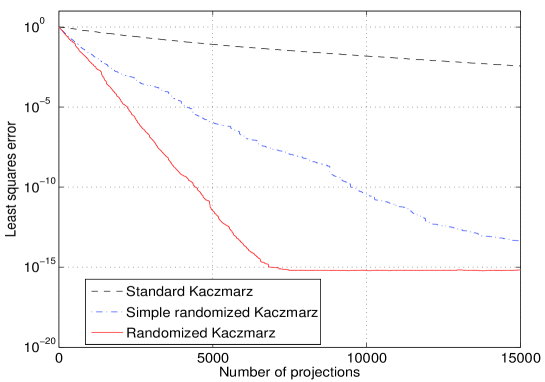
Figure 1: Comparison of rate of convergence for the randomized Kaczmarz method described in Algorithm 1 and other Kaczmarz methods applied to the nonuniform sampling problem described in the main text.

4.2 Comparison to conjugate gradient algorithm

In recent years conjugate gradient (CG) type methods have emerged as the leading iterative algorithms for solving large linear systems of equations, since they often exhibit remarkably fast convergence [17, 21]. How does Algorithm 1 compare to the CG algorithms?

The rate of convergence of CGLS applied to $Ax=b$ is bounded by [17]

$$\|x_{k}-x\|_{A^{\ast}A}\leq 2\|x_{0}-x\|_{A^{\ast}A}\Big{(}\frac{k(A)-1}{k(A)+1}\Big{)}^{k},$$ (19)

where $\|y\|_{A^{\ast}A}:=\sqrt{\langle Ay,Ay\rangle}$.

It is known that the CG method may converge faster when the singular values of $A$ are clustered [36]. For instance, take a matrix whose singular values, all but one, are equal to one, while the remaining singular value is very small, say $10^{-8}$. While this matrix is far from being well-conditioned, CGLS will nevertheless converge in only two iterations, due to the clustering of the spectrum of $A$, cf. [36]. In comparison, the proposed Kaczmarz method will converge extremely slowly in this example by Theorem 3, since $\kappa(A)\approx 10^{8}$.

On the other hand, Algorithm 1 can outperform CGLS on problems for which CGLS is actually quite well suited, in particular for random Gaussian matrices $A$, as we show below.

Solving random linear systems

Let $A$ be a $m\times n$ matrix whose entries are independent $N(0,1)$ random variables. Condition numbers of such matrices are well studied, when the aspect ratio $y:=n/m<1$ is fixed and the size $n$ of the matrix grows to infinity. Then the following almost sure convergence was proved by Geman [16] and Silvestein [35] respectively:

$$\frac{\|A\|_{2}}{\sqrt{m}}\to 1+\sqrt{y};\qquad\frac{1/\|A^{-1}\|_{2}}{\sqrt{m}}\to 1-\sqrt{y}.$$

Hence

$$k(A)\to\frac{1+\sqrt{y}}{1-\sqrt{y}}.$$ (20)

Also, since $\frac{\|A\|_{F}}{\sqrt{mn}}\to 1$, we have

$$\frac{\kappa(A)}{\sqrt{n}}\to\frac{1}{1-\sqrt{y}}.$$ (21)

For estimates that hold for each finite $n$ rather than in the limit, see e.g. [11] and [10].

Now we compare the expected computation complexities of the randomized Kaczmarz algorithm proposed in Algorithm 1 and CGLS to compute the solution within error ${\varepsilon}$ for the system (1) with a random Gaussian matrix $A$.

We estimate the expected number of iterations (projections) $k_{\varepsilon}$ for Algorithm 1 to achieve an accuracy ${\varepsilon}$ in (11). Using bound (21), we have

$$\mathbb{E}\,k_{\varepsilon}\approx\frac{2n}{(1-\sqrt{y})^{2}}\log\frac{1}{\varepsilon}$$

as $n\to\infty$. Since each iteration (projection) requires $n$ operations, the total expected number of operations is

$$\text{Complexity of randomized Kaczmarz}\approx\frac{2n^{2}}{(1-\sqrt{y})^{2}}\log\frac{1}{\varepsilon}.$$ (22)

The expected number of iterations $k^{\prime}_{\varepsilon}$ for CGLS to achieve the accuracy ${\varepsilon}$ can be estimated using (19). First note that the norm $\|\cdot\|_{A^{*}A}$ is on average proportional to the Euclidean norm $\|z\|_{2}$. Indeed, for any fixed vector $z$ one has $\mathbb{E}\|z\|_{A^{*}A}^{2}=\mathbb{E}\|Az\|_{2}^{2}=m\|z\|_{2}^{2}$. Thus, when using CGLS for a random matrix $A$, we can expect that the bound (19) on the convergence also holds for the Euclidean norm.

Consequently, the expected number of iterations $k^{\prime}_{\varepsilon}$ in CGLS to compute the solution within accuracy $\varepsilon$ as in (10) is

$$\mathbb{E}k_{\varepsilon}\approx\frac{\log\frac{2}{\varepsilon}}{\log K(A)}\qquad\text{where}\quad K(A)=\frac{k(A)+1}{k(A)-1}.$$

By (20), for random matrices $A$ of growing size we have $K\to 1/\sqrt{y}$ almost surely. Thus

$$\mathbb{E}k_{\varepsilon}\approx\frac{2\log\frac{2}{\varepsilon}}{\log\frac{1}{y}}.$$

The main computational task in each iteration of CGLS consists of two matrix vector multiplications, one with $A$ and one with $A^{\ast}$, each requiring $m\times n=n^{2}/y$ operations. Hence the total expected number of operations is

$$\text{Complexity of CGLS}\approx\frac{4n^{2}}{y\log\frac{1}{y}}\cdot\log\frac{2}{\varepsilon}.$$ (23)

It is easy to compare the complexities (22) and (23) as functions of $y$, since $n^{2}$ and $\log(1/{\varepsilon})$ are common terms in both (using the approximation $\log(2/{\varepsilon})\approx\log(1/{\varepsilon})$ for small ${\varepsilon}$), cf. also Figure 2. A simple computation shows that (22) and (23) are essentially equal when $y\approx\frac{1}{3}$. Hence for Gaussian matrices our analysis predicts that Algorithm 1 outperforms CGLS in terms of computational efficiency when $m>3n$.

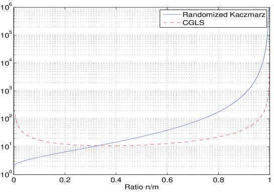
Figure 2: Comparison of the computational complexities (22) (randomized Kaczmarz method) and (23) (conjugate gradient algorithm) as functions of the ratio $y=\frac{n}{m}$ (the common factors $n^{2}$ and $\log(1/{\varepsilon})$ in (22) and (23) are ignored in the two curves).

While the computational cost of Algorithm 1 decreases as $\frac{n}{m}$ decreases, this is not the case for CGLS. Therefore it is natural to ask for the optimal ratio $\frac{n}{m}$ for CGLS for Gaussian matrices that minimizes its overall computational complexity. It is easy to see that for given ${\varepsilon}$ the expression in (23) is minimized if $y=1/e$, where $e$ is Euler’s number. Thus if we are given an $m\times n$ Gaussian matrix (with $m>en$), the most efficient strategy to employ CGLS is to first select a random submatrix $A^{(e)}$ of size $en\times n$ from $A$ (and the corresponding subvector $b^{(e)}$ of $b$) and apply CGLS to the subsystem $A^{(e)}x=b^{(e)}$. This will result in the optimal computational complexity $4en^{2}\log\frac{2}{{\varepsilon}}$ for CGLS.

Thus for a fair comparison between the randomized Kaczmarz method and CGLS, we will apply CGLS in our numerical simulations to both the “full” system $Ax=b$ as well as to a subsystem $A^{(e)}x=b^{(e)}$, where $A^{(e)}$ is an $en\times n$ submatrix of $A$, randomly selected from $A$.

In the first simulation we let $A$ be of dimension $300\times 100$, the entries of $x$ are also drawn from a normal distribution. We apply both, CGLS and Algorithm 1. We apply CGLS to the full system of size $300\times 100$ as well as to a randomly selected subsystem of size $272\times 100$ (representing the optimal size $en\times n$, computed above). Since we know the true solution we can compute the actual least squares error $\|x-x_{k}\|$ after each iteration. Each method is terminated after reaching the required accuracy ${\varepsilon}=10^{-14}$. We repeat the experiment 100 times and for each method average the resulting least squares errors.

In Figure 3 we plot the averaged least squares error (y-axis) versus the number of floating point operations (x-axis), cf. Figure 3. We also plot the estimated convergence rate for both methods. Recall that our estimates predict essentially identical bounds on the convergence behavior for CGLS and Algorithm 1 for the chosen parameters ($m=3n$). Since in this example the performance of CGLS applied to the full system of size $300\times 100$ is almost identical to that of CGLS applied to the subsystem of size $272\times 100$, we display only the results of CGLS applied to the original system.

While CGLS performs somewhat better than the (upper) bound predicts, Algorithm 1 shows a significantly faster convergence rate. In fact, the randomized Kaczmarz method is almost twice as efficient as CGLS in this example.

In the second example we let $m=500,n=100$. In the same way as before, we illustrate the convergence behavior of CGLS and Algorithm 1. In this example we display the convergence rate for CGLS applied to the full system (labeled as CGLS full matrix) of size $500\times 100$ as well as to a random subsystem of size $272\times 100$ (labeled as CGLS submatrix). As is clearly visible in Figure 4 CGLS applied to the subsystem provides better performance than CGLS applied to the full system, confirming our theoretical analysis. Yet again, Algorithm 1 is even more efficient than predicted, this time outperforming CGLS by a factor of 3 (instead of a factor of about 2 according to our theoretical analysis).

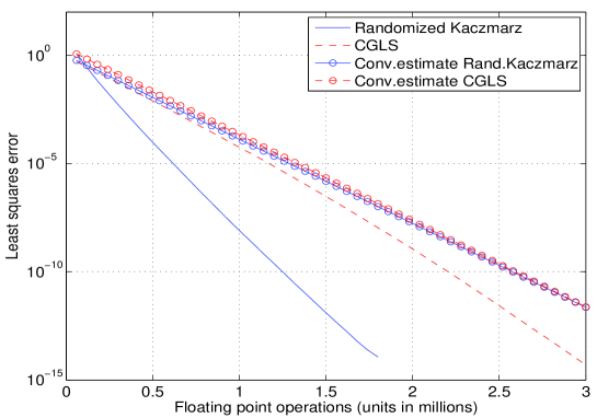
Figure 3: Comparison of rate of convergence for the randomized Kaczmarz method described in Algorithm 1 and the conjugate gradient least squares algorithm for a system of equations with a Gaussian matrix of size $300\times 100$.

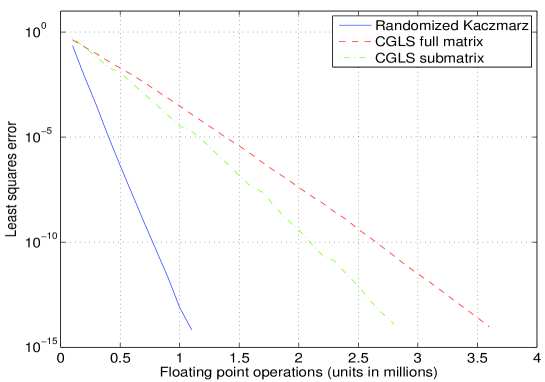
Figure 4: Comparison of rate of convergence for the randomized Kaczmarz method described in Algorithm 1 and the conjugate gradient least squares algorithm for a system of equations with a Gaussian matrix of size $500\times 100$.

Remark: An important feature of the conjugate gradient algorithm is that its computational complexity reduces significantly when the complexity of the matrix-vector multiplication is much smaller than ${\mathcal{O}}(mn)$, as is the case e.g. for Toeplitz-type matrices. In such cases conjugate gradient algorithms will outperform Kaczmarz type methods.

5 Some open problems

In this final section we briefly discuss a few loose ends and some open problems.

Kaczmarz method with relaxation: It has been observed that the convergence of the Kaczmarz method can be accelerated by introducing relaxation. In this case the iteration rule becomes

$$x_{k+1}=x_{k}+\lambda_{k,i}\frac{b_{i}-\langle a_{i},x_{k}\rangle}{\|a_{i}\|_{2}^{2}}a_{i},$$ (24)

where the $\lambda_{k,i}$, $i=1,\dots,m$ are relaxation parameters. For consistent systems the relaxation parameters must satisfy [25]

$$0<{\operatorname{liminf}}_{k\to\infty}\lambda_{k,i}\leq{\operatorname{limsup}}_{k\to\infty}\lambda_{k,i}<2$$ (25)

to ensure convergence.

We have observed in our numerical simulations that for instance for Gaussian matrices a good choice for the relaxation parameter is to set $\lambda_{k,i}:=\lambda=1+\frac{n}{m}$ for all $k$ and $i$. While we do not have a proof for an improvement of performance or even optimality, we provide the result of a numerical simulation that is typical for the behavior we have observed, cf. Figure 5.

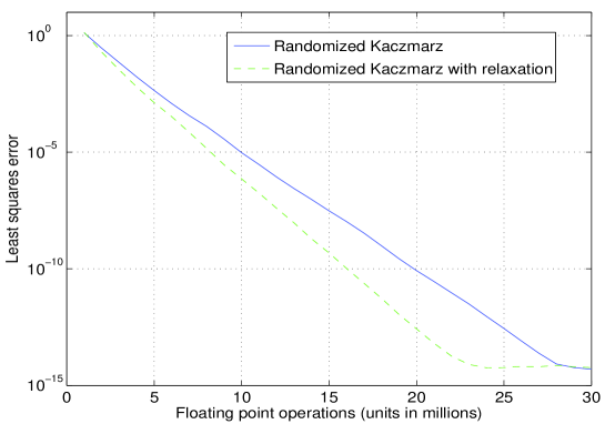
Figure 5: Comparison of rate of convergence for the randomized Kaczmarz method with and without relaxation parameter. We have used $\lambda=1+\frac{n}{m}$ as relaxation parameter.

Inconsistent systems: Many systems arising in practice are inconsistent due to noise that contaminates the right hand side. In this case it has been shown that convergence to the least squares solution can be obtained with (strong under)relaxation [5, 22]. We refer to [22, 23] for suggestions for the choice of the relaxation parameter as well as further in-depth analysis for this case.

While our theoretical analysis presented in this paper assumes consistency of the system of equations, it seems quite plausible that the randomized Kaczmarz method combined with appropriate underrelaxation should also be useful for inconsistent systems.

References

- [1] R. F. Bass, K. Gröchenig, Random sampling of multivariate trigonometric polynomials. SIAM J. Math. Anal. 36 (2004/05), no. 3, 773–795
- [2] J. J. Benedetto and P. J. S. G. Ferreira, editors. Modern sampling theory. Applied and Numerical Harmonic Analysis. Birkhäuser Boston Inc., Boston, MA, 2001. Mathematics and applications.
- [3] R.L. Burden and J.D. Faires. Numerical Analysis. Brooks/Cole Publ.Co., eighth edition, 2006.
- [4] C. Cenker, H. G. Feichtinger, M. Mayer, H. Steier, and T. Strohmer. New variants of the POCS method using affine subspaces of finite codimension, with applications to irregular sampling. In Proc. SPIE: Visual Communications and Image Processing, pages 299–310, 1992.
- [5] Y. Censor, P.P.B. Eggermont, and D. Gordon. Strong underrelaxation in Kaczmarz’s method for inconsistent linear systems. Numer. Math., 41:83–92, 1983.
- [6] J. Demmel, The probability that a numerical analysis problem is difficult. Math. Comp. 50 (1988), no. 182, 449–480
- [7] F. Deutsch. Rate of convergence of the method of alternating projections. In Parametric optimization and approximation (Oberwolfach, 1983), volume 72 of Internat. Schriftenreihe Numer. Math., pages 96–107. Birkhäuser, Basel, 1985.
- [8] F. Deutsch and H. Hundal. The rate of convergence for the method of alternating projections. II. J. Math. Anal. Appl., 205(2):381–405, 1997.
- [9] A. Edelman. Eigenvalues and condition numbers of random matrices. SIAM J. Matrix Anal. Appl., 9(4):543–560, 1988.
- [10] A. Edelman. On the distribution of a scaled condition number. Math. Comp. 58 (1992), no. 197, 185–190.
- [11] A. Edelman, B. D. Sutton. Tails of condition number distributions. SIAM J. Matrix Anal. Appl. 27 (2005), no. 2, 547–560
- [12] H. G. Feichtinger and K. Gröchenig. Error analysis in regular and irregular sampling theory. Applicable Analysis, 50:167–189, 1993.
- [13] H. G. Feichtinger, K. Gröchenig, and T. Strohmer. Efficient numerical methods in non-uniform sampling theory. Numerische Mathematik, 69:423–440, 1995.
- [14] A. Frieze, R. Kannan, and S. Vempala. Fast monte-carlo algorithms for finding low-rank approximations. Proceedings of the Foundations of Computer Science, 39:378–390, 1998. Journal version in Journal of the ACM 51 (2004), 1025-1041.
- [15] A. Galántai. On the rate of convergence of the alternating projection method in finite dimensional spaces. J. Math. Anal. Appl., 310(1):30–44, 2005.
- [16] S. Geman. Limit theorem for the norm of random matrices. Ann. Probab., 8(2):252–261, 1980.
- [17] G.H. Golub and C.F. van Loan. Matrix Computations. Johns Hopkins, Baltimore, third edition, 1996.
- [18] Ulf Grenander and Jack W. Silverstein. Spectral analysis of networks with random topologies. SIAM J. Appl. Math., 32(2):499–519, 1977.
- [19] K. Gröchenig. Reconstruction alrorithms in irregular sampling. Math. Comp. 59 (1992), 181–194.
- [20] K. Gröchenig. Irregular sampling, Toeplitz matrices, and the approximation of entire functions of exponential type. Math. Comp., 68:749–765, 1999.
- [21] M. Hanke. Conjugate gradient type methods for ill-posed problems. Longman Scientific & Technical, Harlow, 1995.
- [22] M. Hanke and W. Niethammer. On the acceleration of Kaczmarz’s method for inconsistent linear systems. Lin. Alg. Appl., 130:83–98, 1990.
- [23] M. Hanke and W. Niethammer. On the use of small relaxation parameters in Kaczmarz’s method. Z. Angew. Math. Mech., 70(6):T575–T576, 1990. Bericht über die Wissenschaftliche Jahrestagung der GAMM (Karlsruhe, 1989).
- [24] G.T. Herman. Image reconstruction from projections. Academic Press Inc. [Harcourt Brace Jovanovich Publishers], New York, 1980. The fundamentals of computerized tomography, Computer Science and Applied Mathematics.
- [25] G.T. Herman, A. Lent, and P.H. Lutz. Relaxation methods for image reconstruction. Commun. Assoc. Comput. Mach., 21:152–158, 1978.
- [26] G.T. Herman and L.B. Meyer. Algebraic reconstruction techniques can be made computationally efficient. IEEE Transactions on Medical Imaging, 12(3):600–609, 1993.
- [27] G.N. Hounsfield. Computerized transverse axial scanning (tomography): Part I. description of the system. British J. Radiol., 46:1016–1022, 1973.
- [28] S. Kaczmarz. Angenäherte Auflösung von Systemen linearer Gleichungen. Bull. Internat. Acad. Polon.Sci. Lettres A, pages 335–357, 1937.
- [29] V. Marchenko and L. Pastur. The eigenvalue distribution in some ensembles of random matrices. Math. USSR Sbornik, 1:457–483, 1967.
- [30] F. Natterer. The Mathematics of Computerized Tomography. Wiley, New York, 1986.
- [31] M. Rudelson and R. Vershynin. Sampling from large matrices: an approach through geometric functional analysis, 2006. Submitted.
- [32] M. Rudelson and R. Vershynin. Invertibility of random matrices. I. The smallest singular value is of order . Preprint.
- [33] M. Rudelson and R. Vershynin. Invertibility of random matrices. II. The Littlewood-Offord theory. Preprint.
- [34] K.M. Sezan and H. Stark. Applications of convex projection theory to image recovery in tomography and related areas. In H. Stark, editor, Image Recovery: Theory and application, pages 415–462. Acad. Press, 1987.
- [35] J. W. Silverstein, The smallest eigenvalue of a large-dimensional Wishart matrix. Ann. Probab. 13 (1985), no. 4, 1364–1368.
- [36] A. van der Sluis and H.A. van der Vorst. The rate of convergence of conjugate gradients. Numer. Math., 48:543–560, 1986.
- [37] D. A. Spielman, S.-H. Teng. Smoothed analysis of algorithms. Proceedings of the International Congress of Mathematicians, Vol. I (Beijing, 2002), 597–606, Higher Ed. Press, Beijing, 2002
- [38] T. Tao, V. Vu. Inverse Littlewood-Offord theorems and the condition number of random discrete matrices. Annals of Mathematics, to appear
- [39] Kenneth W. Wachter. The strong limits of random matrix spectra for sample matrices of independent elements. Ann. Probability, 6(1):1–18, 1978.
- [40] S. Yeh and H. Stark. Iterative and one-step reconstruction from nonuniform samples by convex projections. J. Opt. Soc. Amer. A, 7(3):491–499, 1990.