Abstract

In [1], the authors consider the generalization ${\mathcal{G}^{\vee}_{K}}$ of the Erdős-Rényi random graph process ${\mathcal{G}_{1}}$, where instead of adding new edges uniformly, ${\mathcal{G}^{\vee}_{K}}$ gives a weight of size $1$ to missing edges between pairs of isolated vertices, and a weight of size $K\in[0,\infty)$ otherwise. This can correspond to the linking of settlements or the spreading of an epidemic. The authors investigate $t^{\vee}_{g}(K)$, the critical time for the appearance of a giant component as a function of $K$, and prove that $t_{g}^{\vee}=\left(1+o(1)\right)\frac{4}{\sqrt{3K}}$, using a proper timescale.

In this work, we show that a natural variation of the model ${\mathcal{G}^{\vee}_{K}}$ has interesting properties. Define the process ${\mathcal{G}^{\wedge}_{K}}$, where a weight of size $K$ is assigned to edges between pairs of non-isolated vertices, and a weight of size $1$ otherwise. We prove that the asymptotical behavior of the giant component threshold is essentially the same for ${\mathcal{G}^{\wedge}_{K}}$, and namely $t^{\wedge}_{g}/t^{\vee}_{g}$ tends to $\frac{64\sqrt{6}}{\pi(24+\pi^{2})}\approx 1.47$ as $K\to\infty$. However, the corresponding thresholds for connectivity satisfy $t^{\wedge}_{c}/t^{\vee}_{c}=\max\{\frac{1}{2},K\}$ for every $K>0$. Following the methods of [1], $t^{\wedge}_{g}$ is characterized as the singularity point to a system of differential equations, and computer simulations of both models agree with the analytical results as well as with the asymptotic analysis. In the process, we answer the following question: when does a giant component emerge in a graph process where edges are chosen uniformly out of all edges incident to isolated vertices, while such exist, and otherwise uniformly? This corresponds to the value of $t^{\wedge}_{g}(0)$, which we show to be $\frac{3}{2}+\frac{4}{3\mathrm{e}^{2}-1}$.

1 Introduction

1.1 The Erdős-Rényi graph process and biased processes

The random graph process, ${\mathcal{G}_{1}}(n)$, is a sequence of $\binom{n}{2}+1$ graphs on $n$ vertices, ${\mathcal{G}_{1}}^{0},\ldots,{\mathcal{G}_{1}}^{\binom{n}{2}}$, where ${\mathcal{G}_{1}}^{0}$ is the edgeless graph on $n$ vertices, and ${\mathcal{G}_{1}}^{T}$ is obtained by adding an edge to ${\mathcal{G}_{1}}^{T-1}$, chosen uniformly over all missing edges. This model was introduced by Erdős and Rényi in [9], where it is shown that for every constant $C<\frac{1}{2}$, the largest component of ${\mathcal{G}_{1}}^{Cn}$ is typically of size $O(\log n)$, and yet for every constant $C>\frac{1}{2}$ there is typically a single component of linear size in ${\mathcal{G}_{1}}^{Cn}$ and all other components are of size $O(\log n)$. This single component and its evolution are referred to as the “giant component”, and “the double jump phenomenon” respectively. Using a timescale of $n/2$ edges, the threshold for the appearance of the giant component is thus $t_{g}=1$. Another classical result of Erdős and Rényi determines that ${\mathcal{G}_{1}}^{Cn\log n}$ is typically connected for $C>\frac{1}{2}$, and typically disconnected for $C<\frac{1}{2}$. Using a timescale of $\frac{n}{2}\log n$, the connectivity threshold is thus $t_{c}=1$. For further information on the evolution of the giant component in the random graph process, as well as on the threshold for connectivity, see, e.g., [3].

There has been extensive study on the thresholds for the appearance of a giant component and for connectivity in different variations of the random graph process. For instance, in a model suggested by Achlioptas, two random edges are chosen uniformly out of the missing edges at each step, out of which some algorithm $\mathcal{A}$ selects one to be added to the graph. For results on upper and lower bounds on the emerging of the giant components for various algorithms in this model, see [4],[5],[6],[10].

In [7], the authors consider a random graph process on multi-graphs, where at each step an edge is added between a random vertex of minimal degree and a random uniformly chosen vertex. The authors analyze the number of vertices of degrees $0,1,2$ along the process using the differential equation method for graph processes of Wormald [12], and show that the mentioned graph process becomes connected typically when the minimal degree becomes $3$.

The following generalization of the original graph process ${\mathcal{G}_{1}}$, which we denote by ${\mathcal{G}^{\vee}_{K}}(n)$, was studied in [1]: at each step, ${\mathcal{G}^{\vee}_{K}}$ gives a weight of size $1$ to missing edges between pairs of isolated vertices, and a weight of size $K\in[0,\infty)$ otherwise (when no isolated vertices are left, the distribution on the missing edges becomes the uniform distribution). This can correspond to the linking process of $n$ initially isolated settlements, or the spreading of an epidemic, where the probability of a new link is affected by whether or not one of its endpoints already has other links. The threshold for the appearance of a giant component in ${\mathcal{G}^{\vee}_{K}}$, $t^{\vee}_{g}$, becomes a continuous function of the parameter $K$, and the authors of [1] use the differential equation method to express $t^{\vee}_{g}$ as a singularity point to a system of coupled non-linear ordinary differential equations (ODEs). By applying methods of asymptotic analysis of ODEs, it is proved that $t^{\vee}_{g}(K)=\left(1+o(1)\right)\frac{4}{\sqrt{3K}}$, where the $o(1)$-term tends to $0$ as $K\to\infty$.

In this work, we show that a natural variation on the process ${\mathcal{G}^{\vee}_{K}}$ has interesting properties. Consider the process ${\mathcal{G}^{\wedge}_{K}}$, where instead of placing the weight $K$ when one of the endpoints is non-isolated (as in ${\mathcal{G}^{\vee}_{K}}$), it is placed when both endpoints are non-isolated. In other words, ${\mathcal{G}^{\vee}_{K}}$ gives a weight of size $K\in[0,\infty)$ to missing edges between pairs of non-isolated vertices, and a weight of size $1$ otherwise. Notice that for $K=1$, both processes are equivalent to the original graph process. Furthermore, for any $K$, both processes ${\mathcal{G}^{\vee}_{K}}$ and ${\mathcal{G}^{\wedge}_{K}}$ apply the rule of the original graph process ${\mathcal{G}_{1}}$ once no isolated vertices are left, hence it is interesting to compare the two up to roughly that point.

Applying the methods of [1] on ${\mathcal{G}^{\wedge}_{K}}$, we express its threshold for the appearance of a giant component, $t^{\wedge}_{g}(K)$, as a singularity point to a system of coupled non-linear ODEs. For the special case $K=0$, we obtain a setting where edges are added uniformly at random out of all edges incident to an isolated vertex, until no such vertex is left (from that point on, edges are added uniformly at random). In this special case we get $t^{\wedge}_{g}(0)=\frac{3}{2}+\frac{4}{3\mathrm{e}^{2}-1}$.

Using classical methods of asymptotic analysis of ODEs (see, e.g., [2]) we readily calculate the asymptotic behavior of $t^{\wedge}_{g}(K)$ for $K\gg 1$, and obtain that $t^{\wedge}_{g}(K)=\left(1+o(1)\right)\frac{\pi}{2\sqrt{2}}\left(1+\frac{\pi^{2}}{24}\right)\frac{1}{\sqrt{K}}$. It follows that $t^{\wedge}_{g}/t^{\vee}_{g}\approx 1.47$ for $K\gg 1$, and we note that obtaining this result via combinatorial arguments seems challenging. Numerical approximations of the ODEs validate this asymptotic analysis.

While the behavior of the threshold for the appearance of a giant component is similar for $K\gg 1$, combinatorial arguments yield that for all $K>0$, $t^{\vee}_{c}(K)=1$, whereas $t^{\wedge}_{c}(K)=\max\{\frac{1}{2},K\}$, hence $t^{\wedge}_{c}/t^{\vee}_{c}=K$ for every $K\geq\frac{1}{2}$.

It is possible to implement both processes ${\mathcal{G}^{\wedge}_{K}}$ and ${\mathcal{G}^{\vee}_{K}}$ efficiently by choosing an appropriate data-structure for holding the isolated and non-isolated vertices. Our implementation requires $O(n)$ memory and runs in time $O(n\log n)$, and its results validate the above analytical results.

1.2 Notations and main results

A property of graphs is a collection of graphs closed under isomorphism. A property is said to be monotone (increasing) if it is closed under the addition of edges. Throughout the paper, we say that a property of graphs on $n$ vertices occurs with high probability, or almost surely, or that almost every process $\mathcal{G}$ satisfies this property, if the probability for the corresponding event tends to $1$ as $n\to\infty$. Note that, when proving that certain statements hold with high probability, one may clearly condition on events which hold with high probability.

On several occasions, we examine the processes ${\mathcal{G}^{\vee}_{K}}$ or ${\mathcal{G}^{\wedge}_{K}}$ starting from some arbitrary graph $H$ (instead of the edgeless graph). We denote these processes by ${\mathcal{G}^{\vee}_{K}}|_{H}$ and ${\mathcal{G}^{\wedge}_{K}}|_{H}$.

Given a process $\mathcal{G}$, we let $\mathcal{G}^{i}$ denote $\mathcal{G}$ after $i$ edges. It will be convenient to use two timescales when referring to $\mathcal{G}$, which we denote by:

$$\mathcal{G}(t) := \mathcal{G}^{tn/2}~{},$$

$$\mathcal{G}[t] := \mathcal{G}^{t\frac{n}{2}\log n}~{}.$$

We say that $t$ is a threshold for the appearance of a giant component in $\mathcal{G}$ if for every $\varepsilon>0$, with high probability $\mathcal{G}(t-\varepsilon)$ does not contain a giant component and yet $\mathcal{G}(t+\varepsilon)$ does contain one. Similarly, we say that $t$ is a threshold for connectivity if for every $\varepsilon>0$, with high probability $\mathcal{G}[t-\varepsilon]$ is disconnected whereas $\mathcal{G}[t+\varepsilon]$ is connected. According to these definitions, both thresholds equal $1$ for the original random graph process ${\mathcal{G}_{1}}$.

Theorem 1.1 determines the threshold for connectivity in both processes, $t^{\vee}_{c}$ and $t^{\wedge}_{c}$, and shows that $t^{\vee}_{c}=1$ for any $K>0$ whereas $t^{\wedge}_{c}=K$ for any $K>\frac{1}{2}$, hence their ratio is $K$ for any $K>\frac{1}{2}$. Furthermore, as we later state, it follows from [1] that a ratio of $\lceil\max\{\frac{1}{K},K\}\rceil$ is the maximal possible between the threshold of ${\mathcal{G}^{\wedge}_{K}}$ and the threshold of ${\mathcal{G}_{1}}$ for any monotone property, and therefore, $t^{\vee}_{c}$ achieves this maximum.

Theorem 1.1.

For every $K>0$, $t^{\vee}_{c}(K)=1$ and yet $t^{\wedge}_{c}(K)=\max\{\frac{1}{2},K\}$. In the special case $K=0$ we have $t^{\vee}_{c}(0)=t^{\wedge}_{c}(0)=\frac{1}{2}$.

For a given graph $G=(V,E)$ on $|V|=n$ vertices, we let $\mathcal{C}=\mathcal{C}(G)$ denote the set of connected components of $G$, and for $i\in\mathbb{N}$, we define $\mathcal{C}_{i}=\mathcal{C}_{i}(G)$ to be the set of components of size $i$: $\mathcal{C}_{i}=\{C\in\mathcal{C}(G):|C|=i\}$. Whenever it is clear as to which graph process $\mathcal{G}$ we are referring, we use the abbreviation $\mathcal{C}_{i}^{t}$ to denote $\mathcal{C}_{i}(\mathcal{G}^{t})$. The fractions of vertices which belong to components of size $1$ and $2$ are defined as:

$$I(G)=\frac{|\mathcal{C}_{1}|}{n}~{},~{}I_{2}(G)=\frac{2|\mathcal{C}_{2}|}{n}~{},$$

and the susceptibility of $G$, $S(G)$, is defined to be the average size of a connected component, averaged over all vertices:

$$S(G)=\frac{1}{n}\sum_{v\in V}|C(v)|=\frac{1}{n}\sum_{C\in\mathcal{C}(G)}|C|^{2},$$

where $C(v)$ denotes the connected component of $v$. The relation between $S(G)$ and the existence of a giant component in $G$ is immediate: if $G$ contains a component of size $\alpha n$ for some $\alpha>0$, then $S(G)\geq\alpha^{2}n$, and if $S(G)\geq\alpha n$ then clearly there exists a component of size $\alpha n$. Therefore, $G$ has a giant component iff $S(G)=\Theta(n)$.

The methods used in [1] to analyze ${\mathcal{G}^{\vee}_{K}}$ and describe $t^{\vee}_{g}$ as a singularity point to a system of ODEs can in fact be applied to a wider class of graph processes. Namely, these methods can be applied to every process where the weight function $W$ on the missing edges satisfies $\max W/\min W\leq K$ for some constant $K>0$. Instead of repeating the complete set of arguments of [1] in order to prove analogous results on ${\mathcal{G}^{\wedge}_{K}}$, we summarize the arguments briefly, and proceed to prove the necessary conditions required for them to work.

Following the ideas of [1] and previously of [10], define the following system of coupled ODEs:

$$\left\{\begin{array}[]{lcl}y^{\prime}&=&\displaystyle{\frac{-y}{1+(K-1)(1-y)^{2}}}\\ y(0)&=&1\\ \end{array}\right.~{},$$ (3)

$$\left\{\begin{array}[]{lcl}z^{\prime}&=&\displaystyle{\frac{z^{2}+(K-1)(z-y)^{2}}{1+(K-1)(1-y)^{2}}}\\ z(0)&=&1\\ \end{array}\right.~{}.$$ (6)

We further define:

$$\left\{\begin{array}[]{lcl}w^{\prime}&=&\displaystyle{\frac{y^{2}-2wy-2Kw(1-y)}{1+(K-1)(1-y)^{2}}}\\ w(0)&=&0\\ \end{array}\right.~{},$$ (7)

where $y$ is the solution to (3). Theorem 1.2 states that $I(G)$, $S(G)$ and $I_{2}(G)$ along the process ${\mathcal{G}^{\wedge}_{K}}$ are approximated by the solutions to the ODEs above, and that $t^{\wedge}_{g}$ is equal to the singularity point of the solution to (6) for any $K>0$:

Theorem 1.2.

Let $y(t)$, $z(t)$ and $w(t)$ denote the solutions for (3),(6),(7), and let $x_{c}$ denote the singularity point of $z(t)$ if such exists, and $\infty$ otherwise. For $0<\delta<1$, let $\tau_{\delta}>0$ be the minimal point satisfying $y(\tau_{\delta})\leq\delta$. The following statements hold almost surely:

1. For every $\delta>0$, $\left|I\left({\mathcal{G}^{\wedge}_{K}}(t)\right)-y(t)\right|=o(1)$ and $\left|I_{2}\left({\mathcal{G}^{\wedge}_{K}}(t)\right)-w(t)\right|=o(1)$ for all $0\leq t\leq\tau_{\delta}$.

2. For every $\varepsilon,\delta>0$, $\left|S\left({\mathcal{G}^{\wedge}_{K}}(t)\right)-z(t)\right|=o(1)$ for all $0\leq t\leq\min\{\tau_{\delta},x_{c}-\varepsilon\}$.

3. For all $K>0$, $t^{\wedge}_{g}=x_{c}$.

The value of $t^{\wedge}_{g}$ in the special case $K=0$ and the asymptotic behavior of $t^{\wedge}_{g}$ are stated in the following theorem:

Theorem 1.3.

The threshold for the appearance of a giant component, $t^{\wedge}_{g}(K)$, is a continuous function of $K$ on $(0,\infty)$, and satisfies:

$$\left\{\begin{array}[]{lcl}t^{\wedge}_{g}(0)&=&\frac{3}{2}+\frac{4}{3\mathrm{e}^{2}-1}\\ t^{\wedge}_{g}(K)&=&\left(1+o(1)\right)\frac{\pi}{2\sqrt{2}}\left(1+\frac{\pi^{2}}{24}\right)\frac{1}{\sqrt{K}}\\ \end{array}\right.~{},$$

where the $o(1)$-term tends to $0$ as $K\to\infty$.

The rest of this paper is organized as follows: in Section 2, we prove Theorem 1.1 by examining second moments of processes which are easier to analyze, and provide results of computer simulations of $t^{\vee}_{c}$ and $t^{\wedge}_{c}$. In Section 3, we prove Theorems 1.2 and 1.3 using analysis of differential equations, and provide results of computer simulations of $t^{\wedge}_{g}$.

2 Thresholds for connectivity

The proof of Theorem 1.1 uses the following result of [1]:

Definition.

Let $M\in\mathbb{N}$. An $M$-bounded weighted graph process on $n$ vertices, $\mathcal{H}=\mathcal{H}(n)$, is an infinite sequence of graphs on $n$ vertices, $(\mathcal{H}^{0},\mathcal{H}^{1},\ldots)$, where $\mathcal{H}^{0}$ is some fixed initial graph, and $\mathcal{H}^{t}$ is generated from $\mathcal{H}^{t-1}$ by adding one edge at random, according to a distribution of the following type: the probability of adding the edge $e$ to $\mathcal{H}^{t-1}$ is proportional to some weight function $W_{t}(e)$, satisfying:

$$\max_{e\notin\mathcal{H}^{t-1}}W_{t}(e)\leq M\min_{e\notin H^{t-1}}W_{t}(e)~{}.$$

If for some $\nu\geq 0$ $\mathcal{H}^{\nu}=K_{n}$, we define $\mathcal{H}^{t}=\mathcal{H}^{\nu}=K_{n}$ for every $t>\nu$.

Theorem 2.1 ([1]).

Let $\mathcal{H}$ denote an $M$-bounded weighted graph process on $n$ vertices, and let $\mathcal{A}$ denote a monotone increasing property of graphs on $n$ vertices. The following statements hold for any $t\in\mathbb{N}$:

$$\Pr[\mathcal{H}^{t}\in\mathcal{A}] \leq \Pr[{\mathcal{G}_{1}}^{Mt}|_{\mathcal{H}^{0}}\in\mathcal{A}]~{},$$ (8)

$$\Pr[{\mathcal{G}_{1}}^{t}|_{\mathcal{H}^{0}}\in\mathcal{A}] \leq \Pr[\mathcal{H}^{Mt}\in\mathcal{A}]~{}.$$ (9)

Notice that for every $K>0$, the processes ${\mathcal{G}^{\vee}_{K}}$ and ${\mathcal{G}^{\wedge}_{K}}$ are both $M$-bounded, where $M=\lceil\max\{\frac{1}{K},K\}$. As it is well-known that $I(t)$, the fraction of isolated vertices is $(1+o(1))\exp(-C)$ at time $Cn/2$, Theorem 2.1 implies that the for any fixed $C$ and $K>0$, ${\mathcal{G}^{\vee}_{K}}(C)$ and ${\mathcal{G}^{\wedge}_{K}}(C)$ almost surely contain $\Theta(n)$ isolated vertices. On the other hand, it is not difficult to see that ${\mathcal{G}^{\vee}_{0}}(1)$ has at most $1$ isolated vertex, and we will later show that ${\mathcal{G}^{\wedge}_{0}}(\frac{3}{2}+o(1))$ almost surely has no isolated vertices. For this reason, we treat the cases $K>0$ and $K=0$ separately. Lemmas 2.2 and 2.3 below establish the precise behavior of these parameters when $K>0$:

Lemma 2.2.

Let $K>0$. For every $0<\varepsilon<1$, ${\mathcal{G}^{\vee}_{K}}[1+\varepsilon]$ is almost surely connected, whereas ${\mathcal{G}^{\vee}_{K}}[1-\varepsilon]$ is almost surely disconnected. Altogether, $t^{\vee}_{c}=1$.

Lemma 2.3.

Let $K>0$. For every $0<\varepsilon<1$, ${\mathcal{G}^{\wedge}_{K}}[(1+\varepsilon)\max\{\frac{1}{2},K\}]$ is almost surely connected, whereas ${\mathcal{G}^{\wedge}_{K}}[K-\varepsilon]$ and ${\mathcal{G}^{\wedge}_{K}}[\frac{1}{2}-\varepsilon]$ are almost surely disconnected. Altogether, $t^{\wedge}_{c}=\max\{\frac{1}{2},K\}$.

As we stated in the introduction, combining the fact that $t_{c}=1$ for ${\mathcal{G}_{1}}$ with Theorem 2.1 yields that $t^{\wedge}_{c}(K)\leq\lceil\max\{\frac{1}{K},K\}\rceil$, and indeed Lemma 2.3 shows that for $K\geq 1$, $K\in\mathbb{N}$, this maximum is achieved.

The remaining case $K=0$ is settled by the next lemma:

Lemma 2.4.

The threshold for connectivity for $K=0$ satisfies $t^{\vee}_{c}(0)=t^{\wedge}_{c}(0)=\frac{1}{2}$.

2.1 Proof of Lemma 2.2

Let $0<\varepsilon<1$; we first show that $t^{\vee}_{c}\leq 1+\varepsilon$. It is easy and well known that for every $\varepsilon^{\prime}>0$, there exists some $c=c(\varepsilon^{\prime})$ such that, with high probability, ${\mathcal{G}_{1}}(c)$ has a giant component of size at least $(1-\varepsilon^{\prime})n$: assume that indeed this holds. Take $0<\varepsilon^{\prime}<\displaystyle{\min\{\frac{\varepsilon/4}{1+\varepsilon},K\}}$ and $c=c(\varepsilon^{\prime})$ as above, and notice that:

$$\frac{1-\varepsilon^{\prime}}{1+\varepsilon^{\prime}}\geq\frac{1+\frac{\varepsilon}{2}}{1+\varepsilon}~{}.$$ (10)

By Theorem 2.1, the giant component of ${\mathcal{G}^{\vee}_{K}}^{c^{\prime}n/2}$ typically contains at least $(1-\varepsilon^{\prime})n$ vertices, where $c^{\prime}=\lceil\max\{K,\frac{1}{K}\}\rceil c$. Let $H^{i}$ denote the largest component of ${\mathcal{G}^{\vee}_{K}}^{i}$, and let $A_{v}^{i}$, $v\in V$, denote the event: $(v\notin H^{i})$. The following holds for every $i\geq c^{\prime}n/2$:

$$\Pr[\neg A_{v}^{i+1}|A_{v}^{i}]=\frac{K|H^{i}|}{K(\binom{n}{2}-i)-(K-1)\binom{|\mathcal{C}_{1}^{i}|}{2}}\geq\frac{K(1-\varepsilon^{\prime})n}{K\binom{n}{2}+\binom{|\mathcal{C}_{1}^{i}|}{2}}\geq\frac{1-\varepsilon^{\prime}}{(1+\varepsilon^{\prime})\frac{n}{2}}~{},$$ (11)

where the last inequality is by the fact that $\frac{|\mathcal{C}_{1}^{i}|}{n}\leq\varepsilon^{\prime}<K$. Setting $T_{0}=c^{\prime}n/2$, this gives the following upper bound on $A_{v}^{T}$ for $v\notin H^{T_{0}}$:

$$\Pr[A_{v}^{T}|\neg A_{v}^{T_{0}}]=\prod_{j=T_{0}}^{T}\Pr[A_{v}^{j}|A_{v}^{j-1}]\leq\prod_{j=T_{0}}^{T}\left(1-\frac{1-\varepsilon^{\prime}}{(1+\varepsilon^{\prime})\frac{n}{2}}\right)\leq$$

$$\leq\exp\left(-(T-T_{0})\frac{1-\varepsilon^{\prime}}{(1+\varepsilon^{\prime})\frac{n}{2}}\right)~{}.$$ (12)

Thus, for $T=(1+\varepsilon)\frac{n}{2}\log n$ we get:

$$\Pr[A_{v}^{T}]\leq\exp\left(-\frac{1-\varepsilon^{\prime}}{1+\varepsilon^{\prime}}\left((1+\varepsilon)\log n-c^{\prime}\right)\right)\leq\exp\left(-(1+\frac{\varepsilon}{2})\log n+O(1)\right)=o(n^{-1})~{},$$

hence a union bound on the vertices of $V\setminus H^{T_{0}}$ implies that, with high probability, ${\mathcal{G}^{\vee}_{K}}[1+\varepsilon]$ is connected.

The lower bound on $t^{\vee}_{c}$ is slightly more delicate. A simple way to show the lower bound in ${\mathcal{G}_{1}}$ is to apply a second moment argument on the number of isolated vertices of ${\mathcal{G}_{1}}(1)$. However, in the case of ${\mathcal{G}^{\vee}_{K}}$, using uniform upper and lower bounds on $\mathcal{C}_{1}^{i}$ (such as $\varepsilon^{\prime}n$ and $o(n)$) does not yield useful bounds on the above second moment. The following claim resolves this difficulty:

Claim 2.5.

Let $0<\delta<\frac{1}{2}$, and let $\{H_{0}\}_{n}$ denote a family of arbitrary graphs on $n$ vertices with $(1+o(1))n^{1-\delta}$ isolated vertices. If $\mathcal{H}$ is a biased ${\mathcal{G}^{\vee}_{K}}$ process on $n$ vertices which begins with $H_{0}$, that is: $\mathcal{H}\sim{\mathcal{G}^{\vee}_{K}}|_{H_{0}}$, then $\mathcal{H}[1-2\delta]$ almost surely contains isolated vertices.

Indeed, to obtain the lower bound on $t^{\vee}_{c}$ from the above claim, fix $\delta=\varepsilon/2$, and let $\tau$ denote the minimal time at which $\mathcal{C}_{1}^{\tau}\leq n^{1-\delta}$. Taking $H_{0}={\mathcal{G}^{\vee}_{K}}^{\tau}$, Claim 2.5 implies that ${\mathcal{G}^{\vee}_{K}}|_{H_{0}}$ almost surely has isolated vertices at time $\tau+(1-2\delta)\frac{n}{2}\log n$, and in particular, we obtain that $t^{\vee}_{c}\geq 1-\varepsilon$, as required. It remains to prove Claim 2.6:

Proof of claim.

Let $H_{0}$ and $\delta$ be as above, and let $\mathcal{H}\sim{\mathcal{G}^{\vee}_{K}}|_{H_{0}}$. Let $B_{u}^{i}$ denote the event that the vertex $u$ is isolated at time $i$, where $i\leq n\log n$. Clearly:

$$\Pr[\neg B_{u}^{i+1}|B_{u}^{i}]=\frac{K(n-|\mathcal{C}_{1}^{i}|)+(|\mathcal{C}_{1}^{i}|-1)}{K(\binom{n}{2}-i)-(K-1)\binom{|\mathcal{C}_{1}^{i}|}{2}}~{}.$$

By the assumption on $H_{0}$, $|\mathcal{C}_{1}^{i}|\leq|\mathcal{C}_{1}^{0}|=(1+o(1))n^{1-\delta}$, thus:

$$\Pr[\neg B_{u}^{i+1}|B_{u}^{i}]=\frac{2+O(n^{-\delta})}{n\left(1+O(\frac{\log n}{n})+O(n^{-2\delta})\right)}=\frac{2+O(n^{-\delta})}{n}~{}.$$ (13)

Similarly, we can define $B_{u,v}^{i}=B_{u}^{i}\wedge B_{v}^{i}$ for $i\leq n\log n$ and get:

$$\Pr[\neg B_{u,v}^{i+1}|B_{u,v}^{i}]=\frac{2K(n-|\mathcal{C}_{1}^{i}|)+2(|\mathcal{C}_{1}^{i}|-2)+1}{K(\binom{n}{2}-i)-(K-1)\binom{|\mathcal{C}_{1}^{i}|}{2}}=\frac{4+O(n^{-\delta})}{n}~{}.$$ (14)

Let $T=(1-2\delta)\frac{n}{2}\log n$, and define $Y=\sum_{u}\mathbf{1}_{B_{u}^{T}}=|\mathcal{C}_{1}^{T}|$ to be the number of isolated vertices of $\mathcal{H}^{T}$. A straightforward second moment consideration implies that $Y>0$ almost surely. To see this, first note that (13) along with the well known bound $1-x\geq\mathrm{e}^{-x/(1-x)}$ for $0\leq x<1$ yield:

$$\mathbb{E}Y=|\mathcal{C}_{1}^{0}|\prod_{i=1}^{T}\Pr[B_{u}^{i}|B_{u}^{i-1}]=(1+o(1))n^{1-\delta}\left(1-\frac{2+O(n^{-\delta})}{n}\right)^{T}\geq$$

$$\geq(1+o(1))n^{1-\delta}\exp\left(-\frac{\left(2+o(1)\right)/n}{1-\frac{2+o(1)}{n}}(1-2\delta)\frac{n}{2}\log n\right)=n^{1-\delta}n^{-1+2\delta+o(1)}=n^{\delta+o(1)}~{}.$$ (15)

By (13) and (14), there exist $p=p(n)$ and $q=q(n)$ such that $\Pr[\neg B_{u,v}^{i+1}|B_{u,v}^{i}]\geq p=\frac{4+O(n^{-\delta})}{n}$ and $\Pr[\neg B_{u}^{i+1}|B_{u}^{i}]\leq q=\frac{2+O(n^{-\delta})}{n}$. The following holds:

$$\mathrm{Cov}(\mathbf{1}_{B_{u}^{T}},\mathbf{1}_{B_{v}^{T}})=\Pr[B_{u,v}^{T}]-\Pr[B_{u}^{T}]^{2}\leq(1-p)^{T}-(1-q)^{2T}=$$

$$=\left(1-p-(1-q)^{2}\right)\sum_{i=0}^{T-1}(1-p)^{i}(1-q)^{2(T-1-i)}=\frac{O(n^{-\delta})}{n}T\left(1-\frac{4+o(1))}{n}\right)^{T-1}\leq$$

$$\leq(1-2\delta)\log n\cdot O(n^{-\delta})\exp\left(-(1+o(1))\frac{4}{n}(1-2\delta)\frac{n}{2}\log n\right)=n^{-2+3\delta+o(1)}~{}.$$

Therefore,

$$\sum_{u\in\mathcal{C}_{1}^{0}}\sum_{v\in\mathcal{C}_{1}^{0}}\mathrm{Cov}(\mathbf{1}_{B_{u}^{T}},\mathbf{1}_{B_{v}^{T}})\leq n^{2(1-\delta)}n^{-2+3\delta+o(1)}=n^{\delta+o(1)}=o\left((\mathbb{E}Y)^{2}\right)~{}.$$

As $\mathrm{E}Y=\omega(1)$, applying Chebyshev’s inequality gives:

$$\Pr[Y=0]\leq\frac{\mathrm{Var}Y}{(\mathbb{E}Y)^{2}}\leq\frac{\mathbb{E}Y+\sum_{u}\sum_{v}\mathrm{Cov}(\mathbf{1}_{B_{u}^{T}},\mathbf{1}_{B_{v}^{T}})}{(\mathbb{E}Y)^{2}}=\frac{1}{\mathbb{E}Y}+o(1)=o(1)~{}.$$

This completes the proof of the claim and of Lemma 2.2. ∎

2.2 Proof of Lemma 2.3

Let $0<\varepsilon<1$. The bounds $t^{\wedge}_{c}\leq(1+\varepsilon)\max\{\frac{1}{2},K\}$ and $t^{\wedge}_{c}\geq K-\varepsilon$ will follow from arguments similar to the ones in the proof of Lemma 2.2, whereas the bound $t^{\wedge}_{c}\geq\frac{1}{2}-\varepsilon$ requires more work.

To prove that $t^{\wedge}_{c}\leq(1+\varepsilon)\max\{\frac{1}{2},K\}$, take $\varepsilon^{\prime}>0$ which satisfies:

$$\left\{\begin{array}[]{ll}\displaystyle{(1-\varepsilon^{\prime})\geq\frac{\left(1+\varepsilon/4\right)^{2}}{1+\varepsilon}}\\ \displaystyle{1-(1-\varepsilon^{\prime})^{2}+(1-\varepsilon^{\prime})^{2}K<\left(1+\frac{\varepsilon}{4}\right)K}\end{array}\right.~{}.$$ (16)

For instance, the following choice is suitable:

$$\varepsilon^{\prime}<\min\left\{\frac{\varepsilon K}{4},1-\sqrt{1-\frac{\varepsilon}{2}\min\{K,1\}}\right\}~{}.$$

As before, take $c=c(\varepsilon^{\prime})$ such that, with high probability, ${\mathcal{G}_{1}}(c)$ has a giant component of size at least $(1-\varepsilon^{\prime})n$. Defining $H^{i}$ to be the largest component of ${\mathcal{G}^{\wedge}_{K}}^{i}$, Theorem 2.1 implies that $|H^{c^{\prime}n/2}|\geq(1-\varepsilon^{\prime})n$ with high probability, where $c^{\prime}=\lceil\max\{K,\frac{1}{K}\}\rceil c$, and therefore we may assume that this indeed holds. Let $A_{u}^{i}$ denote the event that a vertex $u\in V\setminus H^{i}$, which belongs to some connected component $C$, joins the giant component at time $i+1$. The following holds:

$$\Pr[A_{u}^{i}]=\frac{|H^{i}|w_{C}}{\binom{n}{2}+(K-1)\binom{n-|\mathcal{C}_{1}^{i}|}{2}-Ki}\mbox{ , where }w_{C}=\left\{\begin{array}[]{cl}1&\mbox{if }|C|=1\\ K|C|&\mbox{otherwise}\end{array}\right.~{}.$$ (17)

By the choice of $c^{\prime}$, for all $i\geq c^{\prime}n/2$ we get:

$$\Pr[A_{u}^{i}]\geq\frac{w_{C}(1-\varepsilon^{\prime})n}{\binom{n}{2}+(K-1)\binom{n-|\mathcal{C}_{1}^{i}|}{2}}\geq\frac{2w_{C}(1-\varepsilon^{\prime})}{n\left(1-(1-\frac{|\mathcal{C}_{1}^{i}|}{n})^{2}+K(1-\frac{|\mathcal{C}_{1}^{i}|}{n})^{2}\right)}~{}.$$

For $K\geq 1$, the denominator in the expression above is clearly bounded from above by $nK$, and for $0<K<1$ it is bounded from above by $n\left(1-(1-\varepsilon^{\prime})^{2}+(1-\varepsilon^{\prime})^{2}K\right)$, hence (16) implies:

$$\Pr[A_{u}^{i}]\geq\frac{2w_{C}(1-\varepsilon^{\prime})}{nK(1+\varepsilon/4)}\geq\frac{2w_{C}(1+\varepsilon/4)}{nK(1+\varepsilon)}~{}.$$ (18)

Take $T_{0}=c^{\prime}n/2$ and $T=\max\{\frac{1}{2},K\}(1+\varepsilon)\frac{n}{2}\log n$, and define the following event for every $u\notin H^{T_{0}}$:

$$B_{u}^{T}=(u\notin H^{T})~{}.$$

The definition of $w_{C}$ in (17) implies that $w_{C}\geq\min\{1,2K\}$ and when combined with (18) this gives:

$$\Pr[B_{u}^{T}]\leq\prod_{i=T_{0}}^{T}\left(1-\frac{2\min\{1,2K\}(1+\varepsilon/4)}{nK(1+\varepsilon)}\right)\leq$$

$$\leq\exp\left(-\frac{1+\varepsilon/4}{1+\varepsilon}\cdot\frac{\min\{\frac{1}{K},2\}}{n/2}\left(\max\{\frac{1}{2},K\}(1+\varepsilon)\frac{n}{2}\log n-c^{\prime}\frac{n}{2}\right)\right)=n^{-(1+\varepsilon/4)+o(1)}~{}.$$

Therefore, the expected number of vertices of $V\setminus H^{T_{0}}$ which do not join $H^{T}$ is clearly $o(1)$, implying that ${\mathcal{G}^{\wedge}_{K}}[(1+\varepsilon)\max\{\frac{1}{2},K\}]$ is almost surely connected.

The lower bound $t^{\wedge}_{c}\geq K-\varepsilon$ follows from the following claim, analogous to Claim 2.5:

Claim 2.6.

Let $0<\delta<\frac{1}{2}$, and let $\{H_{0}\}_{n}$ denote a family of arbitrary graphs on $n$ vertices with $(1+o(1))n^{1-\delta}$ isolated vertices. If $\mathcal{H}\sim{\mathcal{G}^{\wedge}_{K}}|_{H_{0}}$, then $\mathcal{H}[K-2\delta]$ almost surely contains isolated vertices.

Proof.

As in the proof of Claim 2.5, let $B_{u}^{i}$ denote the event ($u$ is isolated at time $i$) and let $B_{u,v}^{i}=B_{u}^{i}\wedge B_{v}^{i}$, where $u,v\in V(H_{0})$. Clearly:

$$\Pr[\neg B_{u}^{i+1}|B_{u}^{i}]=\frac{n-1}{\binom{n}{2}+(K-1)\binom{n-|\mathcal{C}_{1}^{i}|}{2}-Ki}~{}.$$

The assumption on $H_{0}$ gives $|\mathcal{C}_{1}^{i}|\leq|\mathcal{C}_{1}^{0}|=(1+o(1))n^{1-\delta}$, and thus for all $i=O(n\log n)$:

$$\Pr[\neg B_{u}^{i+1}|B_{u}^{i}]=\frac{2}{Kn\left(1+O(\frac{\log n}{n})+O(n^{-\delta})\right)}=\frac{2+O(n^{-\delta})}{Kn}~{},$$ (19)

and:

$$\Pr[\neg B_{u,v}^{i+1}|B_{u,v}^{i}]=\frac{2n-3}{\binom{n}{2}+(K-1)\binom{n-|\mathcal{C}_{1}^{i}|}{2}-Ki}=\frac{4+O(n^{-\delta})}{Kn}~{}.$$ (20)

Henceforth, a similar calculation to the one in the proof of Claim 2.5 gives the required result. ∎

Choosing $\delta=\varepsilon/2$ and applying the last claim implies that $t^{\wedge}_{c}\geq K-\varepsilon$, and it remains to show that $t^{\wedge}_{c}\geq\frac{1}{2}-\varepsilon$. This follows from the fact that ${\mathcal{G}^{\wedge}_{K}}[\frac{1}{2}-\varepsilon]$ contains components of size $2$ almost surely. Unfortunately, we cannot repeat the last argument in order to show that indeed this is the case, since we have no guarantee that at time $\tau$, the hitting time for the property $|\mathcal{C}_{1}|\leq n^{1-\delta}$, ${\mathcal{G}^{\wedge}_{K}}$ still satisfies $|\mathcal{C}_{2}|=n^{1-\alpha}$ for some small $\alpha$. To prove the next claim, which completes the proof of Lemma 2.2, we consider a simplified process, where it is possible to give a lower bound on $|\mathcal{C}_{2}|$, and show that this process stochastically dominates ${\mathcal{G}^{\wedge}_{K}}$ with regards to $|\mathcal{C}_{2}|$.

Claim 2.7.

For all $K\in(0,1]$ and $\varepsilon>0$, ${\mathcal{G}^{\wedge}_{K}}[\frac{1}{2}-\varepsilon]$ almost surely contains a connected component of size $2$.

Proof of claim.

Define the process ${\widetilde{\mathcal{G}^{\wedge}_{K}}}$, which is an approximated version of ${\mathcal{G}^{\wedge}_{K}}$, as follows: at each step, assign a weight $K$ to ordered pairs of the form $\{(u,v):u,v\notin\mathcal{C}_{1}\}$, and a weight $1$ otherwise. If the ordered pair $(u,v)$ chosen at some step $i$ is a (self) loop or corresponds to an edge which already exists in ${\widetilde{\mathcal{G}^{\wedge}_{K}}}$, this step is omitted. In other words, ${\widetilde{\mathcal{G}^{\wedge}_{K}}}$ assigns weights to all ordered pairs, and disregards selections of multiple edges or loops. Clearly, if ${\widetilde{\mathcal{G}^{\wedge}_{K}}}^{t}$ contains $m\leq t$ edges, then ${\widetilde{\mathcal{G}^{\wedge}_{K}}}^{t}\sim{\mathcal{G}^{\wedge}_{K}}^{m}$. Furthermore, for any $t=o(n^{2})$ we have:

$$\mathbb{E}\left(t-|E({\widetilde{\mathcal{G}^{\wedge}_{K}}}^{t})|\right)\leq\sum_{i=1}^{t}\max\{\frac{1}{K},K\}\frac{t+n}{n^{2}}=\left(O\left(\frac{t}{n^{2}}\right)+O\left(\frac{1}{n}\right)\right)t=o(t)~{},$$

where $E(H)$ denotes the set of edges of the graph $H$. In particular, for any fixed $c$, with high probability ${\mathcal{G}^{\wedge}_{K}}(c)\sim{\widetilde{\mathcal{G}^{\wedge}_{K}}}(c+o(1))$ and ${\mathcal{G}^{\wedge}_{K}}[c]\sim{\widetilde{\mathcal{G}^{\wedge}_{K}}}[c+o(1)]$, and it is sufficient to prove the claim for ${\widetilde{\mathcal{G}^{\wedge}_{K}}}$.

Take $0<\varepsilon<\frac{1}{2}$. By well known results on the original Erdős-Rényi graph process, for any fixed $t$, with high probability: $|\mathcal{C}_{2}({\mathcal{G}_{1}}(t))|=\Theta(n)$, with the constant tending to $0$ as $t\to\infty$. For a short proof of this fact, one can verify that the following differential equation approximates the graph parameter $I_{2}$ along ${\mathcal{G}_{1}}$ up to an $o(1)$ error term:

$$w^{\prime}(t)=-2w(t)+y^{2}(t)~{},~{}w(0)=0~{},$$

where $y(t)$ is the approximating function of the fraction of isolated vertices, $I(t)$, and the time-scaling is of $n/2$ edges at each step. Substituting the well known fact (which also follows from Theorem 1.2 when substituting $K=1$) that $y(t)=\exp(-t)$, it follows that $w(t)=t\exp(-2t)$.

By Theorem 2.1 and the above fact, we deduce that for every sufficiently large $c$ there exist $0<\alpha_{1}<\alpha_{2}<\frac{1}{3}$ such that ${\widetilde{\mathcal{G}^{\wedge}_{K}}}(c)$ almost surely satisfies $\alpha_{1}n\leq|\mathcal{C}_{2}|\leq\alpha_{2}n$. Let:

$$c^{\prime}=\inf\{t>c:y(t)\leq\frac{\varepsilon K}{2}\}~{},$$

where $y$ is the solution to the ODE (3)), and set $\varepsilon^{\prime}=y(c^{\prime})$. By Theorem 1.2, with high probability $I\left({\widetilde{\mathcal{G}^{\wedge}_{K}}}(c^{\prime})\right)=y(c^{\prime})+o(1)$, and in particular, ${\widetilde{\mathcal{G}^{\wedge}_{K}}}(c^{\prime})$ has $(1+o(1))\varepsilon^{\prime}n$ isolated vertices almost surely. Let $H_{0}$ denote ${\widetilde{\mathcal{G}^{\wedge}_{K}}}(c^{\prime})$, and take $\alpha_{1}=\alpha_{1}(c^{\prime})$, $\alpha_{2}=\alpha_{2}(c^{\prime})$ as above. According to these definitions, $S=\mathcal{C}_{1}(H_{0})$ satisfies $s=|S|=(1+o(1))\varepsilon^{\prime}n$ almost surely, and $W=\mathcal{C}_{2}(H_{0})$ satisfies $\alpha_{1}n\leq|W|\leq\alpha_{2}n$ almost surely. Assume that indeed this holds.

We consider the graph process $\mathcal{H}$, which begins with $H_{0}$, and at each step selects an ordered pair $(u,v)\in V(H_{0})^{2}$ according to the following probabilities:

$$\left\{\begin{array}[]{ll}\frac{1}{Kn^{2}}&\mbox{if $(u,v)$ is incident to $W$ and $S$}\\ \frac{1}{n^{2}}&\mbox{if $(u,v)$ is incident to $W$ and $V\setminus S$}\\ \lambda&\mbox{otherwise}\end{array}\right.~{},$$

where the value of $\lambda>0$ is chosen such that the probabilities sum up to $1$. This is possible, since the probabilities for the first two types of pairs sum up to at most:

$$2\alpha_{2}\left(\varepsilon^{\prime}/K+(1-\varepsilon^{\prime})\right)\leq 3\alpha_{2}<1~{},$$

as $\varepsilon^{\prime}\leq\frac{K}{2}$ and $\alpha_{2}<\frac{1}{3}$. We claim that the following two events occur almost surely, and complete the proof of the claim:

$$\mathcal{C}_{2}(\mathcal{H}[\frac{1}{2}-\varepsilon])\cap W\neq\emptyset~{},$$ (21)

$$\left|\mathcal{C}_{2}(\mathcal{H}[\frac{1}{2}-\varepsilon])\cap W\right|\leq\left|\mathcal{C}_{2}({\widetilde{\mathcal{G}^{\wedge}_{K}}}|_{H_{0}}[\frac{1}{2}-\varepsilon])\cap W\right|~{}.$$ (22)

A standard second moment consideration proves that (21) occurs with high probability. To see this, set: $T=\left(\frac{1}{2}-\varepsilon\right)\frac{n}{2}\log n$, and notice that:

$$\frac{2T}{Kn^{2}}\left(K(n-s-2)+s\right)=\frac{1}{2}(1-2\varepsilon)\left((1-\varepsilon^{\prime})+\frac{\varepsilon^{\prime}}{K}+o(1)\right)\log n=\frac{1}{2}(1-\varepsilon^{\prime\prime}+o(1))\log n$$ (23)

for some $\varepsilon\leq\varepsilon^{\prime\prime}\leq 2\varepsilon$ (by our choice of $\varepsilon^{\prime}$). Next, let the random variable $X_{e}$ ($e\in W$) be the indicator of the event: $\left(e\in\mathcal{C}_{2}(\mathcal{H}[\frac{1}{2}-\varepsilon])\right)$, and let $X=\sum_{e\in W}X_{e}$. The following holds:

$$\Pr[X_{e}=1]=\left(1-\frac{2K(n-s-2)+2s}{Kn^{2}}\right)^{T}~{},$$

$$\Pr[X_{e}=1\wedge X_{e^{\prime}}=1]=\left(1-\frac{4K(n-s-2)-4K+4s}{Kn^{2}}\right)^{T}~{},$$

for every $e,e^{\prime}\in W$. Thus, a calculation similar to the one in the proof of Claim 2.5 gives:

$$\mathbb{E}X\geq|W|\exp\left(-(2-o(1))T\frac{K(n-s-2)+s}{Kn^{2}}\right)\geq|W|n^{(-1+\varepsilon^{\prime\prime})/2+o(1)}=\omega(\sqrt{n})~{},$$

and:

$$\mathrm{Cov}(X_{e},X_{e^{\prime}})\leq\frac{4K}{Kn^{2}}\exp\left(-4\frac{K(n-s-4)+K+s}{Kn^{2}}T\right)\leq 4n^{-3+\varepsilon^{\prime\prime}+o(1)}~{}.$$

Therefore:

$$\sum_{e\in W}\sum_{e^{\prime}\in W}\mathrm{Cov}(X_{e},X_{e^{\prime}})\leq 4|W|^{2}n^{-3+\varepsilon^{\prime\prime}+o(1)}=o(\mathbb{E}X)~{},$$

and in particular, $\mathrm{Var}(X)=(1+o(1))\mathbb{E}X=o\left(\mathbb{E}X)^{2}\right)$ and by Chebyshev’s inequality we deduce that $X>0$ almost surely.

It remains to prove that (22) occurs almost surely. This is achieved by a coupling argument: we claim that there exists a coupling of the processes ${\widetilde{\mathcal{G}^{\wedge}_{K}}}|_{H_{0}}$ and $\mathcal{H}$ whose support consists of pairs $(G_{t},H_{t})$ such that: $G_{t}\sim{\widetilde{\mathcal{G}^{\wedge}_{K}}}|_{H_{0}}^{t}$, $H_{t}\sim\mathcal{H}^{t}$, and $\left(\mathcal{C}_{2}(H_{t})\cap W\right)\subset\left(\mathcal{C}_{2}(G_{t})\cap W\right)$. This clearly holds for $t=0$, and by induction, it remains to extend the coupling from $(G_{t},H_{t})$ to $(G_{t+1},H_{t+1})$. For this purpose, we apply the following lemma of [1] (Lemma 2.2), which was first proved by Strassen [11] in a slightly different setting:

Lemma 2.8 ([1]).

Let $U,V$ be two finite sets, and let $R\subset U\times V$ denote a relation on $U,V$. Let $\mu$ and $\nu$ denote probability measures on $U$ and $V$ respectively, such that the following inequality holds for every $A\subset U$:

$$\mu(A)\leq\nu(\{y\in V:xRy\mbox{ for some }x\in A\})~{}.$$ (24)

Then there exists a coupling $\varphi$ of $\mu,\nu$ whose support is contained in $R$.

Let $U,V$ be the set of all $n^{2}$ ordered pairs selected, representing the next pair selected by $G_{t}$ and $H_{t}$ respectively. Let $\mu$ denote the probability measure of each selection in $U$ by $G_{t}$, and let $\nu$ denote the probability of each selection in $V$ by $H_{t}$. Define:

$$\left\{\begin{array}[]{lcl}X=\mathcal{C}_{2}(G_{t})\cap W&,&X_{u,v}=\mathcal{C}_{2}\left(G_{t}\cup(u,v)\right)\cap W\\ Y=\mathcal{C}_{2}(H_{t})\cap W&,&Y_{x,y}=\mathcal{C}_{2}\left(H_{t}\cup(x,y)\right)\cap W\end{array}\right.~{}.$$

By the induction hypothesis, $Y\subseteq X$, and we define $R$ to be $\{\left((u,v),(x,y)\right):Y_{x,y}\subseteq X_{u,v}\}$.

Clearly, if $(u,v)$ is a loop or an edge which already belongs to $G_{t}$, it has no effect on $X$, and as $Y_{x,y}\subseteq Y\subseteq X$ we get $(u,v)R(x,y)$ for all $x,y$. Furthermore, every $(u,v)$ which is not incident to any $e\in Y$ also satisfies $(u,v)R(x,y)$ for all $x,y$, as the components $(u,v)$ may remove from $X$ already do not belong to $Y$. Therefore, (24) is satisfied for every $A\subset U$ which contains such pairs $(u,v)$.

It remains to prove that (24) holds for sets $A\subset U$ such that $A\cap E(G_{t})=\emptyset$, and $A$ consists entirely of edges incident to edges of $Y$. Let $A=\{e_{1},\ldots,e_{m}\}$, and notice that $e_{i}\notin E(H_{t})$ for all $i$, as $e_{i}$ is incident to some component $e\in Y$ of size $2$ in $H_{t}$, satisfying $e\neq e_{i}$ as $Y\subset E(G_{t})$. Furthermore, for all $i$ we have $e_{i}Re_{i}$, since all components that $e_{i}$ removes from $X$ in $X_{e_{i}}$ are also removed from $Y$ in $Y_{e_{i}}$. Thus, showing that $\mu(e_{i})\leq\nu(e_{i})$ for all $i$ will imply that $A$ satisfies the condition of (24). Indeed, if $e_{i}=(u,v)$ is such that $u,v\notin S$ ($u,v$ are both non-isolated in $H_{0}$), then:

$$\mu(e_{i})=\frac{K}{n^{2}+(K-1)(n-\mathcal{C}_{1}(G^{t}))^{2}}\leq\frac{K}{Kn^{2}}=\nu(e_{i})~{},$$

and otherwise:

$$\mu(e_{i})\leq\frac{1}{n^{2}+(K-1)(n-\mathcal{C}_{1}(G^{t}))^{2}}\leq\frac{1}{Kn^{2}}=\nu(e_{i})~{},$$

by definition of the process $\mathcal{H}$, completing the proof of the claim and the proof of Lemma 2.2. ∎

2.3 Proof of Lemma 2.4

To prove that $t^{\vee}_{c}(0)=\frac{1}{2}$, we recall the following easy facts stated in [1]: by definition, ${\mathcal{G}^{\vee}_{0}}$ adds edges between pairs of isolated vertices until no such pair is left. Hence, after adding $\lfloor n/2\rfloor$ edges there is at most $1$ isolated vertex in ${\mathcal{G}^{\vee}_{K}}$, and ${\mathcal{G}^{\vee}_{K}}$ behaves as ${\mathcal{G}_{1}}$ on $\lfloor n/2\rfloor$ components of size 2 (and possibly $1$ additional isolated vertex). Thus, $t^{\vee}_{g}(0)=1+\frac{1}{2}=\frac{3}{2}$.

Proving a connectivity threshold of $(\frac{1}{2}+o(1))\frac{n}{2}\log n$, we may assume $n$ is even: otherwise, the single isolated vertex from time $\lfloor n/2\rfloor$ becomes connected almost surely at time $\omega(n)$, and its edge set accounts to at most $n-1=o(n\log n)$ edges, not affecting the threshold for connectivity. By the discussion above, for even values of $n$, ${\mathcal{G}^{\vee}_{0}}$ has a linear number of components of size $2$ and no isolated vertices at the time of appearance of the giant component. Thus, we deduce from the arguments used for the proofs of Lemmas 2.2 and 2.3 that, with high probability, ${\mathcal{G}^{\vee}_{0}}[\frac{1}{2}-\varepsilon]$ still contains components of size $2$, whereas ${\mathcal{G}^{\vee}_{0}}[\frac{1}{2}+\varepsilon]$ is connected. Altogether, $t^{\vee}_{c}(0)=\frac{1}{2}$.

It remains to show that $t^{\wedge}_{c}(0)=\frac{1}{2}$. Substituting $K=0$ in equation (3), it reduces to the form:

$$y^{\prime}=\frac{1}{y-2}~{},~{}y(0)=1~{},$$

provided that $y\neq 0$. This yields the solution:

$$y(t)=2-\sqrt{1+2t}~{}.$$ (25)

Notice that $y(t)$ is strictly monotone decreasing, and reaches $0$ at $t=\frac{3}{2}$. Therefore, if we denote by $\tau_{0}({\mathcal{G}^{\wedge}_{0}})$ the minimal time $t$ at which $I\left({\mathcal{G}^{\wedge}_{0}}(t)\right)=0$, Theorem 1.2 implies that for every $0<\delta<1$, $|\tau-\frac{3}{2}|<\delta$ almost surely. To see this, let $x_{0}$ be such that $y(x_{0})=\delta$, and let $x_{1}=\max\{x_{0},\frac{3}{2}-\delta\}$. By Theorem 1.2, with high probability:

$$I({\mathcal{G}^{\wedge}_{0}}(\frac{3}{2}-\delta))\geq I\left({\mathcal{G}^{\wedge}_{0}}(x_{1})\right)=y(x_{1})+o(1)\geq\frac{1}{2}y(x_{1})>0~{},$$

where the second from last inequality holds for sufficiently large values of $n$. On the other hand, $y(x_{1})<\delta$, and hence $I\left({\mathcal{G}^{\wedge}_{0}}(\frac{3}{2}+\delta)\right)\leq I\left({\mathcal{G}^{\wedge}_{0}}(x_{1}+\delta)\right)=0$ almost surely, since each edge eliminates at least one isolated vertex in ${\mathcal{G}^{\wedge}_{0}}$.

Equation (7) takes the following form after substituting $K=0$ and the value of $y(t)$ as it is given in (25), provided that $y\neq 0$:

$$w^{\prime}(t)=\frac{y-2w}{2-y}=2\frac{1-w}{\sqrt{1+2t}}-1~{},~{}w(0)=0~{},$$

which has the solution:

$$w(t)=\frac{5}{4}-\frac{3}{4}\mathrm{e}^{2(1-\sqrt{1+2t})}-\frac{1}{2}\sqrt{1+2t}~{}.$$ (26)

For $t=\frac{3}{2}$ we have $w(t)=\frac{1}{4}-\frac{3}{4\mathrm{e}^{2}}\approx 0.1485$, hence from the discussion above we obtain that $H={\mathcal{G}^{\wedge}_{K}}(\tau)$ almost surely satisfies $I_{2}(H)=\Theta(n)$ (and $I(H)=0$). From that point on, the process ${\mathcal{G}^{\wedge}_{K}}$ is equivalent to ${\mathcal{G}_{1}}|_{H}$, and from the similar arguments to those used in the proofs of Lemmas 2.2 and 2.3 we obtain that $t^{\vee}_{c}(0)=\frac{1}{2}$. ∎

2.4 Computer experiments of $\mathbf{t^{\wedge}_{c}}$ and $\mathbf{t^{\vee}_{c}}$

Maintaining the set of isolated vertices and the edges already added to the process provides all the information needed to add the next edge to ${\mathcal{G}^{\wedge}_{K}}$ and ${\mathcal{G}^{\vee}_{K}}$ at an $O(1)$ cost. In order to recognize the threshold for connectivity, the set of connected components must be efficiently maintained. Our implementation holds the components in linked-lists, according to the Weighted-Union Heuristic (see, e.g., [8] p. 445) which guarantees an average cost of $O(\log n)$ for uniting components.

Figure 1 shows the results of $t^{\wedge}_{c}$ and $t^{\vee}_{c}$ according to simulations of both models on $n=10^{4}$ vertices. The values of $t^{\wedge}_{c}$ and $t^{\vee}_{c}$ were averaged over 100 tests per value of $K$.

Figure 1: Comparison of the numerical results for $t^{\wedge}_{c}$ and $t^{\vee}_{c}$, and estimations of $t^{\wedge}_{c}$ and $t^{\vee}_{c}$ according to computer simulations of the model.

3 The appearance of a giant component in $\mathbf{{\mathcal{G}^{\wedge}_{K}}}$

3.1 Proof of Theorem 1.2

We begin with a short summary of the methods used in [1] to analyze $t^{\vee}_{g}(K)$ for $K>0$. First, the authors prove Theorem 2.1 and deduce that the process ${\mathcal{G}^{\vee}_{K}}$ is stochastically dominated by ${\mathcal{G}_{1}}$, up to a timescale factor of $\lceil\max\{\frac{1}{K},K\}\rceil$. By applying the differential equation method of Wormald [12] to the approximated process ${\widetilde{\mathcal{G}^{\vee}_{K}}}$ (which selects an ordered pair at each step, similar to the process ${\widetilde{\mathcal{G}^{\wedge}_{K}}}$ introduced in the proof of Claim 2.7), the parameters $I(G)$ and $S(G)$ are approximated by $y(t)$ and $z(t)$, solutions to a system of coupled ODEs. Henceforth, a repeated use of Theorem 3.1 of [10], which relates the susceptibility and the appearance of a giant component, implies that the singularity point $z(t)$ is equal to $t^{\vee}_{c}$.

We note that the methods of [1] can be applied to any family of $M$-bounded processes $\mathcal{P}_{M}$ (as referred to in Theorem 2.1) provided that the following conditions hold:

1. Attempting to approximate a fixed number of bounded graph parameters $Y_{1},\ldots,Y_{d}$ (such as $I(G)$ and $I_{2}(G)$) by functions $y_{1},\ldots,y_{d}$ for $1\leq t\leq T$, we require that

   $$\mathbb{E}\frac{Y_{i}(\mathcal{P}_{M}^{t+1})-Y_{i}(\mathcal{P}_{M}^{t})}{2/n}=\frac{dy_{i}}{dt}\left(Y_{1}(\mathcal{P}_{M}^{t}),\ldots,Y_{d}(\mathcal{P}_{M}^{t}),t\right)+\mathrm{err_{y_{i}}(t)}~{},$$ (27)

   for all $i$ and $t$, where $\max_{i,t}\mathrm{err}_{y_{i}}(t)=o(1)$.

2. In addition to the above approximations of $Y_{1},\ldots,Y_{d}$ by $y_{1},\ldots,y_{d}$, when attempting to approximate $S(G)$ by the function $z(t)$ for $1\leq t\leq T$, we require that

   $$\mathbb{E}\frac{S(\mathcal{P}_{M}^{t+1})-S(\mathcal{P}_{M}^{t})}{2/n}=\frac{dz}{dt}\left(Y_{1}(\mathcal{P}_{M}^{t}),\ldots,Y_{d}(\mathcal{P}_{M}^{t}),S(\mathcal{P}_{M}^{t}),t\right)+\mathrm{err_{z}(t)}~{},$$ (28)

   where $\max_{t}\mathrm{err}_{z}(t)=o(1)$.

   To show the above, we may use the fact that with high probability, the largest component is of size $O(\log n)$ as long as $t<x_{c}-\varepsilon$, where $x_{c}$ is a possible singularity point of $z(t)$. This follows from the proof of Theorem 1.3 of [1], which applies to this generalized setting as well.

3. Finally, if the above function $z(t)$ has a singularity point, we require that it is uniformly bounded (regardless of $M$).

If the above 3 conditions hold, we obtain that $Y_{1},\ldots,Y_{d},S$ are within $o(1)$ distance from $y_{1},\ldots,y_{d},z$ along the process $\mathcal{P}_{M}$ for $1\leq t\leq T$. Furthermore, if $z$ has a singularity point at $x_{c}$ and the above conditions hold with $T=x_{c}-\varepsilon$ for any $\varepsilon>0$, it follows that the appearance of a giant component in $\mathcal{P}_{M}$ is at $t=x_{c}$.

We first show that the above 3 conditions hold for $K>0$ under the assumptions of Theorem 1.2. By the well known fact that for any constant $t$, $I({\mathcal{G}_{1}}(t))=\Theta(n)$ almost surely, Theorem 2.1 implies that $\tau_{\delta}$ can be taken to be arbitrarily large. In particular, we can take $\tau_{\delta}>x_{c}$. In order to verify that (27) holds for $I(G)$ and $I_{2}(G)$, let $G$ and $G^{\prime}$ denote ${\mathcal{G}^{\wedge}_{K}}^{t}$ and ${\mathcal{G}^{\wedge}_{K}}^{t+1}$ respectively for some fixed $t$, and let $I=I(G)$ and $I_{2}=I_{2}(G)$. We have:

$$\mathbb{E}\frac{I(G^{\prime})-I(G)}{2/n} = (-1)\frac{I(I-\frac{1}{n})}{1+(K-1)(1-I)^{2}}+(-1)\frac{2I(1-I)}{1+(K-1)(1-I)^{2}}=$$ (29)

$$= \frac{-I}{1+(K-1)(1-I)^{2}}+O(I/n)~{},$$

and:

$$\mathbb{E}\frac{I_{2}(G^{\prime})-I_{2}(G)}{2/n} = \frac{I(I-\frac{1}{n})-2I_{2}I-2KI_{2}(1-I-I_{2})-2KI_{2}(I_{2}-\frac{2}{n})}{1+(K-1)(1-I)^{2}}=$$ (30)

$$= \frac{I^{2}-2I_{2}I-2KI_{2}(1-I)}{1+(K-1)(1-I)^{2}}+O(I/n)+O(I_{2}/n))~{},$$

where in both cases we used the fact that $K>0$ to obtain an upper bound of $o(1)$ on the error term. To prove (28), set $S=S(G)$ and observe that:

$$\mathbb{E}\frac{S(G^{\prime})-S(G)}{2/n}=$$

$$= \frac{n/2}{1+(K-1)(1-I)^{2}}\bigg{(}I(I-\frac{1}{n})\frac{2}{n}+2I\mathop{\sum_{C\in\mathcal{C}}}_{|C|>1}\frac{|C|}{n}\frac{2|C|}{n}+\mathop{\sum_{C_{1}\in\mathcal{C}}}_{|C_{1}|>1}\mathop{\sum_{C_{2}\in\mathcal{C}\setminus\{C_{1}\}}}_{|C_{2}|>1}\frac{K|C_{1}||C_{2}|}{n^{2}}\frac{2|C_{1}||C_{2}|}{n}\bigg{)}=$$ (31)

$$= \frac{2I(S-I)+I^{2}+K(S-I)^{2}}{1+(K-1)(1-I)^{2}}+O(I/n)+O\bigg{(}\mathop{\sum_{C\in\mathcal{C}}}_{|C|>1}\frac{|C|^{4}}{n^{2}}\bigg{)}=$$

$$= \frac{S^{2}+(K-1)(S-I)^{2}}{1+(K-1)(1-I)^{2}}+O(I/n)+O\bigg{(}\mathop{\sum_{C\in\mathcal{C}}}_{|C|>1}\frac{|C|^{4}}{n^{2}}\bigg{)}~{},$$

and the assumption that $|C|=O(\log n)$ gives a bound of $o(1)$ on $\mathrm{err}_{z}$. The next claim therefore completes the statements of Theorem 1.2 for the case $K>0$:

Claim 3.1.

For every $K>0$, $t^{\wedge}_{g}(K)<5$.

Proof.

Consider the case $K\geq 1$, and let $y(t)$ and $z(t)$ denote the solutions to the ODEs (3) and (6) respectively. Recalling that $y(t)\leq 1$ for every $t\geq 0$, (6) yields that $z^{\prime}(t)\geq 0$ provided that $z(t)\geq 1$. Thus, the initial condition $z(0)=1$ implies that $z(t)$ is monotone increasing in $t$, and in particular:

$$z^{\prime}=\frac{z^{2}+(K-1)(z-y)^{2}}{1+(K-1)(1-y)^{2}}\geq\frac{z^{2}+(K-1)z^{2}(1-y)^{2}}{1+(K-1)(1-y)^{2}}=z^{2}~{},$$ (32)

where inequality is by the fact that $y\geq 0$ and $z\geq 1$. By standard considerations in differential analysis , (32) and the initial condition $z(0)=1$ imply that $z(t)\geq\frac{1}{1-t}$ for every $t\geq 0$ (as $\tilde{z}(t)=\frac{1}{1-t}$ satisfies $\tilde{z}^{\prime}=\tilde{z}^{2}$ and $\tilde{z}(0)=1$), and in particular, $t^{\wedge}_{g}\leq 1$ for any $K\geq 1$.

We are left with the case $0<K<1$. Clearly, (3) implies that $y^{\prime}\leq 0$ for every $t\geq 0$, and furthermore, $y^{\prime}<0$ as long as $y>0$, hence $y$ is strictly monotone decreasing from $1$ to $0$. Let $t^{*}$ be such that

$$y(t^{*})=1-\sqrt{1-K}~{}.$$ (33)

Notice that the solutions to the equation $-x^{2}+2x-\frac{K}{1-K}=0$ are: $x_{1,2}=1\pm\sqrt{1-\frac{K}{1-K}}$ if $0<K\leq\frac{1}{2}$, and no solution exists if $\frac{1}{2}<K<1$. In both cases, $-x^{2}+2x-\frac{K}{1-K}<0$ for every $x\leq 1-\sqrt{1-K}$. Therefore, the definition of $t^{*}$ and the fact that $y$ is monotone decreasing give:

$$-y(t)^{2}+2y(t)-\frac{K}{1-K}\leq 0~{}\mbox{ for every }t\geq t^{*},$$

or equivalently:

$$(1-K)y(t)(2-y(t))\leq K~{}\mbox{ for every }t\geq t^{*}~{}.$$ (34)

Rewriting equation (6) as:

$$z^{\prime}=\frac{z^{2}-(1-K)(z-y)^{2}}{1-(1-K)(1-y)^{2}}=\frac{Kz^{2}+(1-K)y(2z-y)}{K+(1-K)y(2-y)}~{},$$ (35)

it follows that for every $t\geq t^{*}$, $z^{\prime}\geq\frac{1}{2}z^{2}$. Furthermore, for every $t\geq 0$, $z^{\prime}>0$, and hence $z(t^{*})>z(0)=1$. We obtain that the function $w(t)=z(t-t^{*})$ satisfies $w^{\prime}\geq\frac{1}{2}w^{2}$ for every $t\geq 0$ and $w(0)\geq 1$, and by the same consideration as above, $w(t)\geq\frac{2}{2-t}$ for every $t\geq 0$. Altogether, we deduce that $t^{\wedge}_{g}\leq t^{*}+2$, and it remains to provide an upper bound on $t^{*}$.

For this purpose, define $u(t)=1-y(t)$, and consider (3) for $0\leq t\leq t^{*}$:

$$u^{\prime}=-y^{\prime}=\frac{1-u}{1-(1-K)u^{2}}\geq\frac{1-u}{1-u^{4}}=\frac{1}{1+u+u^{2}+u^{3}}~{},$$

where the inequality is by the fact that $u(t)\leq\sqrt{1-K}$ for $0\leq t\leq t^{*}$. Define $w(t)$ to be the solution to the differential equation:

$$w^{\prime}=\frac{1}{1+w+w^{2}+w^{3}}~{},~{}w(0)=0~{},$$ (36)

it follows from the above mentioned argument that $u(t)\geq w(t)$ for $0\leq t\leq t^{*}$. The solution to (36) satisfies: $t=\sum_{j=1}^{4}\frac{w^{j}}{j}$, hence $w(t_{0})=\sqrt{1-K}$ for $t_{0}=\sum_{j=1}^{4}\frac{(1-K)^{j/2}}{j}\leq\frac{25}{12}$. As $u(t_{0})\geq w(t_{0})$, it follows that $t^{*}\leq t_{0}\leq\frac{25}{12}$, completing the proof. ∎

In the special case $K=0$, ${\mathcal{G}^{\wedge}_{0}}$ is no longer an $M$-bounded process, however the assertions of statements $1,2$ of Theorem 1.2 remain valid and follow from (27) and (28), by applying Wormald’s differential equation method directly. To see that (27) holds, notice that as long as $I({\mathcal{G}^{\wedge}_{K}}(t))\geq\delta$ for some fixed $\delta>0$, the denominators in (29) and (30) are $\Theta(1)$, and the approximation remains valid (note that $z(t)$ has no singularity point for $K=0$). To show that (28) holds, set $S=S(G)$, and note that:

$$\mathbb{E}\frac{S(G^{\prime})-S(G)}{2/n} = \frac{n/2}{1-(1-I)^{2}}\bigg{(}I(I-\frac{1}{n})\frac{2}{n}+2I\mathop{\sum_{C\in\mathcal{C}}}_{|C|>1}\frac{|C|}{n}\frac{2|C|}{n}\bigg{)}=$$ (37)

$$= \frac{2I(S-I)+I^{2}}{2I-I^{2}}+O(I/n)=\frac{2S-I}{2-I}+O(I/n)~{},$$

where we used the fact that $I>0$ for $t\leq\tau_{\delta}$. This implies that the error term $\mathrm{err}_{z}$ is $o(1)$ without making any assumptions on the size of the largest component, and completes the proof of the theorem. ∎

3.2 Computer experiments of $\mathbf{t^{\wedge}_{g}}$

We conducted simulations of $t^{\wedge}_{g}$ using the implementation of ${\mathcal{G}^{\wedge}_{K}}$ mentioned in 2.4. In these simulations, the number of vertices was $n=10^{6}$, and the threshold for the appearance of the giant component was taken to be the minimal time at which ${\mathcal{G}^{\wedge}_{K}}$ contains a component of size $\alpha n$, where $\alpha=0.01$. The value of $t^{\wedge}_{g}(K)$ was averaged over $10$ tests for each value of $K$.

Figure 2 shows the comparison between the values of $t^{\wedge}_{g}$ according to the above computer simulations, and the values obtained by numerically solving the ODEs (3) and (6) by Mathematica.

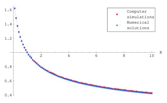
Figure 2: Comparison of the numerical results for $t^{\wedge}_{g}$, and estimations of $t^{\wedge}_{g}$ according to computer simulations of the model.

3.3 Proof of Theorem 1.3

First, the fact that $t^{\wedge}_{c}(K)$ is continuous follows from the general continuous dependence of ODEs on their parameters (in this case,the single parameter $K$).

For the special case $K=0$, recall that in our treatment of ${\mathcal{G}^{\wedge}_{0}}$ for the proof of Lemma 2.4 we showed that for every $\delta>0$, with high probability $y(t)=2-\sqrt{1+2t}$ approximates $I({\mathcal{G}^{\wedge}_{0}}(t))$ for $t\leq\frac{3}{2}-\delta$, and $I({\mathcal{G}^{\wedge}_{0}}(\frac{3}{2}+\delta))=0$. Take $\delta>0$ and consider the interval $[0,\frac{3}{2}-\delta]$; equation (6) takes the following form when substituting $K=0$ and the solution to $y(t)$:

$$z^{\prime}=\frac{z^{2}-(z-y)^{2}}{2y-y^{2}}=\frac{2z-y}{2-y}=\frac{2(z-1)}{\sqrt{1+2t}}+1~{}.$$ (38)

Taking $w=z-1$, we obtain the linear equation:

$$w^{\prime}-\frac{2}{\sqrt{1+2t}}w=1~{}.$$ (39)

Multiplying (39) by its integrating factor and integrating by parts, we get:

$$w(t)=\exp\left\{2\int(1+2t)^{-\frac{1}{2}}dt\right\}\int\exp\left\{-2\int(1+2t)^{-\frac{1}{2}}dt\right\}\,dx~{}=$$

$$=-\frac{1}{2}(\sqrt{1+2t}+\frac{1}{2})+C\exp(2\sqrt{1+2t})~{}.$$

The initial condition $w(0)=0$ gives $C=\frac{3}{4}\mathrm{e}^{-2}$, hence:

$$z(t)=\frac{3}{4}\mathrm{e}^{2(\sqrt{1+2t}-1)}-\frac{1}{2}\sqrt{1+2t}+\frac{3}{4}\mbox{ for all }t\in[0,\frac{3}{2}-\delta]~{}.$$

The above solutions for $y(t)$ and $z(t)$ give $y(\frac{3}{2})=0$ and

$$z(3/2)=\frac{3}{4}\mathrm{e}^{2}-\frac{1}{4}~{}.$$ (40)

Let $\tau_{0}=\tau_{0}({\mathcal{G}^{\wedge}_{0}})$ denote the first time $t$ at which ${\mathcal{G}^{\wedge}_{0}}^{t}$ has no isolated vertices, i.e., the hitting time for the property: $\{G:I(G)=0\}$. By the above arguments, we have:

$$\tau_{0}=\left(\frac{3}{2}+o(1)\right)n/2$$ (41)

almost surely. We claim that proving that with high probability:

$$S({\mathcal{G}^{\wedge}_{0}}^{\tau_{0}})=z(3/2)+o(1)$$ (42)

implies the required result on $t^{\wedge}_{g}(0)$. Indeed, once no isolated vertices are left, the process ${\mathcal{G}^{\wedge}_{0}}$ adds edges according to the uniform distribution, and hence from that point the susceptibility follows the equation $z^{\prime}=z^{2}$ (e.g., see the case $K=1$ of the analysis of ${\mathcal{G}^{\wedge}_{K}}$ or ${\mathcal{G}^{\vee}_{K}}$). By (41), we obtain that for some $x_{c}>\frac{3}{2}$:

$$S({\mathcal{G}^{\wedge}_{0}}(t))=(1+o(1))\frac{1}{x_{c}-t}\mbox{ for any }\frac{3}{2}\leq t<x_{c}~{},$$

and the value of $x_{c}$ is derived from the initial condition (40):

$$t^{\wedge}_{g}(0)=x_{c}=\frac{3}{2}+\frac{4}{3\mathrm{e}^{2}-1}~{}.$$ (43)

It is left to show that (42) indeed holds. The lower bound $S({\mathcal{G}^{\wedge}_{0}}^{\tau_{0}})\geq z(\frac{3}{2})-o(1)$ follows from Theorem 1.2, which states that $z$ approximates $S$ until time $\frac{3}{2}-\delta$ for any $\delta>0$, and from the continuity and monotonicity of $z$. That is, for any fixed $\xi>0$, choosing a sufficiently small $\delta>0$ such that $z(\frac{3}{2}-\delta)>z(\frac{3}{2})-\xi$ gives:

$$S\left({\mathcal{G}^{\wedge}_{0}}(\frac{3}{2}-\delta)\right)=z(\frac{3}{2}-\delta)+o(1)>z(\frac{3}{2})-\xi+o(1)~{}.$$

For the upper bound $S({\mathcal{G}^{\wedge}_{0}}^{\tau_{0}})\leq z(\frac{3}{2})-o(1)$ we are required to examine the second moment of $S\left({\mathcal{G}^{\wedge}_{0}}(\frac{3}{2}+\delta)\right)$. Assume by contradiction that:

$$\Pr\left[S\left({\mathcal{G}^{\wedge}_{0}}^{\tau_{0}}\right)>z(\frac{3}{2})+\xi\right]>\alpha\mbox{ for some fixed }\alpha,\xi>0~{},$$ (44)

and choose $\delta>0$ small enough such that:

$$\left(\frac{z(\frac{3}{2})}{\xi/2}\right)^{2}\left(\mathrm{e}^{12\delta}-\mathrm{e}^{2\delta}\right)<\alpha~{}\mbox{ , and: }~{}\left(\mathrm{e}^{4\delta}-1\right)z(\frac{3}{2})\leq\xi/2~{}.$$ (45)

Set $T_{0}=\left(\frac{3}{2}-\delta\right)\frac{n}{2}$ and $T_{1}=\tau_{0}-1$, and note that, with high probability, $\Delta:=\frac{T_{1}-T_{0}}{n/2}$ satisfies $\delta/2\leq\Delta\leq 2\delta$, and therefore we may assume that this holds. We consider ${\mathcal{G}^{\wedge}_{0}}^{T}$ for $T=T_{0},\ldots,T_{1}$, and let $S_{0}=S\left({\mathcal{G}^{\wedge}_{0}}^{T_{0}}\right)$. As $I({\mathcal{G}^{\wedge}_{0}}^{T})>0$, the calculation which yielded (38) gives:

$$\mathbb{E}\left(S({\mathcal{G}^{\wedge}_{0}}^{T+1})~{}|~{}S({\mathcal{G}^{\wedge}_{0}}^{T})\right)=S({\mathcal{G}^{\wedge}_{0}}^{T})+\frac{2}{n}\left(\frac{2(S({\mathcal{G}^{\wedge}_{0}}^{T})-1)}{2-I({\mathcal{G}^{\wedge}_{0}}^{T})}+1\right)~{},$$

and hence:

$$\left(1+\frac{2}{n}\right)S({\mathcal{G}^{\wedge}_{0}}^{T})\leq\mathbb{E}\left(S({\mathcal{G}^{\wedge}_{0}}^{T+1})~{}|~{}S({\mathcal{G}^{\wedge}_{0}}^{T})\right)\leq\left(1+\frac{4}{n}\right)S({\mathcal{G}^{\wedge}_{0}}^{T})~{}.$$

Therefore:

$$\mathrm{e}^{\Delta}S_{0}\leq\mathbb{E}S({\mathcal{G}^{\wedge}_{0}}^{\tau_{0}})\leq\mathrm{e}^{2\Delta}S_{0}~{}.$$

Similarly, we can write the expression for the second moment of $S({\mathcal{G}^{\wedge}_{0}}^{T_{1}})$:

$$\mathbb{E}\left(S({\mathcal{G}^{\wedge}_{0}}^{T+1})^{2}~{}|~{}S({\mathcal{G}^{\wedge}_{0}}^{T})^{2}\right)\leq S({\mathcal{G}^{\wedge}_{0}}^{T})^{2}\left(1+\frac{4}{n}\cdot\frac{3}{2-I({\mathcal{G}^{\wedge}_{0}}^{T})}\right)~{},$$

and hence:

$$\mathbb{E}\left(S({\mathcal{G}^{\wedge}_{0}}^{\tau_{0}})^{2}\right)\leq\mathrm{e}^{6\Delta}S_{0}^{2}~{}.$$

We obtain that:

$$\mathrm{Var}S({\mathcal{G}^{\wedge}_{0}}^{\tau_{0}})\leq\left(\mathrm{e}^{6\Delta}-\mathrm{e}^{\Delta}\right)S_{0}^{2}\leq\left(\mathrm{e}^{12\delta}-\mathrm{e}^{2\delta}\right)S_{0}^{2}~{},$$

where the last inequality is by the fact that $\Delta\leq 2\delta$ almost surely. By (45) and the fact that $S_{0}<z(\frac{3}{2})$ almost surely, this implies that:

$$\mathrm{Var}S({\mathcal{G}^{\wedge}_{0}}^{\tau_{0}})<\alpha\left(\xi/2\right)^{2}~{}.$$ (46)

By (45) we have:

$$\Pr\left[S\left({\mathcal{G}^{\wedge}_{0}}^{\tau_{0}}\right)>z(\frac{3}{2})+\xi\right]\leq\Pr\left[S\left({\mathcal{G}^{\wedge}_{0}}^{\tau_{0}}\right)-\mathbb{E}{\mathcal{G}^{\wedge}_{0}}^{\tau_{0}}>z(\frac{3}{2})\left(1-\mathrm{e}^{4\delta}\right)+\xi\right]\leq$$

$$\leq\Pr\left[|S\left({\mathcal{G}^{\wedge}_{0}}^{\tau_{0}}\right)-\mathbb{E}{\mathcal{G}^{\wedge}_{0}}^{\tau_{0}}|>\xi/2\right]~{},$$

and thus combining Chebyshev’s inequality with (46) gives:

$$\Pr\left[S\left({\mathcal{G}^{\wedge}_{0}}^{\tau_{0}}\right)>z(\frac{3}{2})+\xi\right]<\alpha~{},$$

contradicting the assumption (44).

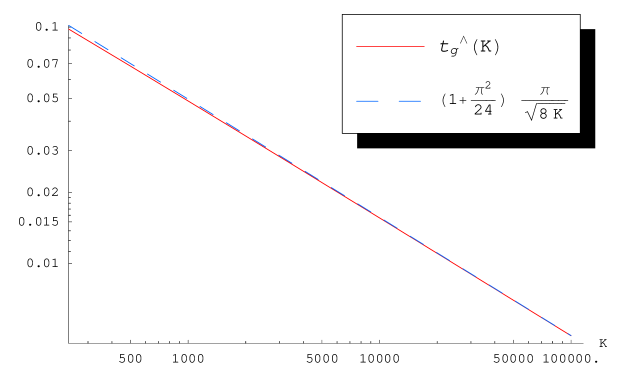
Figure 3: Comparison of the values of $t^{\wedge}_{g}(K)$, obtained by numerical solutions of the ODEs (3)-(6), and the asymptotic approximation of Theorem 1.3. Logarithmic scale was used in both axes.

It remains to show that for $K\gg 1$, $t^{\wedge}_{g}(K)=(1+o(1))\frac{\pi}{2\sqrt{2}}\left(1+\frac{\pi^{2}}{24}\right)\frac{1}{\sqrt{K}}$. Consider equation (3); the initial condition $y(0)=1$ suggests that we examine the function $u(t)=1-y(t)$, which satisfies $u(t)\ll 1$ near the origin:

$$-u^{\prime}=\frac{u-1}{u^{2}(K-1)+1}~{},$$

and substituting the initial condition of $y$ we have:

$$u^{\prime}=\frac{1-u}{u^{2}(K-1)+1}~{},~{}u(0)=0~{}.$$ (47)

As $u\ll 1$, the $u^{2}$-term at the denominator is negligible, and we have:

$$u^{\prime}\approx\frac{1}{Ku^{2}+1}~{},~{}u(0)=0~{},$$ (48)

where here and in what the follows, we denote by $\approx$ equality up to leading order terms. Rearranging the last equation to the form $Ku^{2}u^{\prime}+u^{\prime}\approx 1$ and integrating, we obtain that, up to leading order terms, $u$ satisfies the equation:

$$\frac{K}{3}u^{3}+u\approx t~{}.$$ (49)

We note that this immediately gives $u\approx t$ for $u\ll\frac{1}{\sqrt{K}}$, however we are interested in the behavior of $u$ precisely when $t=\Theta(\frac{1}{\sqrt{K}})$. Applying Caradano’s solution to the above cubic equation gives the following approximation of $u$ when $t\ll 1$ (and hence $u\ll 1)$:

$$u(t)\approx\left(\frac{3t}{2K}+\sqrt{\frac{1}{K^{3}}+\left(\frac{3t}{2K}\right)^{2}}\right)^{1/3}+\left(\frac{3t}{2K}-\sqrt{\frac{1}{K^{3}}+\left(\frac{3t}{2K}\right)^{2}}\right)^{1/3}~{},~{}t\ll 1~{}.$$

Moving on to $z(t)$, we substitute $w=z-1$ in equation (6) and obtain the following:

$$w^{\prime}=\frac{(w+1)^{2}+(K-1)(w+u)^{2}}{1+Ku^{2}-u^{2}}\approx\frac{(w+1)^{2}+(K-1)(w+u)^{2}}{1+Ku^{2}}~{}.$$

Next, we may replace $w+1$ by $1$ whenever $w\ll 1$, and furthermore, whenever $w=\Omega(1)$ clearly the dominant term is $K(w+u)^{2}$. Altogether, we obtain the following uniform approximation for $w$:

$$w^{\prime}\approx\frac{K(w+u)^{2}+1}{Ku^{2}+1}\approx\left(K(w+u)^{2}+1\right)u^{\prime}~{}.$$

Adding $u^{\prime}$ to both sides of the equation and rearranging, we obtain:

$$\frac{w^{\prime}+u^{\prime}}{K(w+u)^{2}+2}\approx u^{\prime}~{},$$

hence if we define $v=\sqrt{\frac{K}{2}}(w+u)$ we obtain:

$$\frac{v^{\prime}}{v^{2}+1}\approx\sqrt{2K}u^{\prime}~{},$$

and thus:

$$v\approx\tan(\sqrt{2K}u)~{}.$$

Returning to $z$, we get:

$$z\approx 1+\sqrt{\frac{2}{K}}\tan(\sqrt{2K}u)-u~{}.$$

This implies that the singularity point $x_{c}$ satisfies $\sqrt{2K}u(x_{c})=\frac{\pi}{2}$. Recalling equation (49), we have:

$$x_{c}\approx\frac{K}{3}u(x_{c})^{3}+u(x_{c})=\frac{K}{3}\frac{\pi^{3}}{16K\sqrt{2K}}+\frac{\pi}{2\sqrt{2K}}=\frac{\pi}{2\sqrt{2}}\left(1+\frac{\pi^{2}}{24}\right)\frac{1}{\sqrt{K}}~{}.$$

Figure 3 shows the excellent agreement between the above asymptotic approximation of $t^{\wedge}_{g}(K)$, and its value as obtained by numerically solving the ODEs (3) and (6) by Mathematica. ∎

Acknowledgement The authors wish to thank Noga Alon for helpful discussions and comments.

References

- [1] G. Amir, O. Gurel-Gurevich, E. Lubetzky, A. Singer, Giant components in biased graph processes, preprint.
- [2] C.M. Bender and S.A. Orszag, Advanced Mathematical Methods for Scientists and Engineers, Springer, New York (1999).
- [3] B. Bollobás, Random graphs, volume 73 of Cambridge Studies in Advanced Mathematics, Cambridge University Press, Cambridge, second edition (2001).
- [4] T. Bohman and A. Frieze, Avoiding a giant component, Random Structures and Algorithms, 19 (2001), 75-85.
- [5] T. Bohman and J.H. Kim, A phase transition for avoiding a giant component, Random Structures and Algorithms , to appear.
- [6] T. Bohman and D. Kravitz, Creating a giant component, Combinatorics, Probability and Computing , to appear.
- [7] M. Kang, Y. Koh, T. Łuczak and S. Ree, The connectivity threshold for the min-degree random graph process, Random Structures and Algorithms, to appear.
- [8] T. H. Cormen, C.E. Leiserson, and R.L. Rivest, Introduction to Algorithms, The MIT Press/McGraw-Hill (1990).
- [9] P. Erdős and A. Rényi, On the evolution of random graphs, Publ. math. Inst. Hungar. Acad. Sci., 5 (1960), 17-61.
- [10] J. Spencer and N. Wormald, Birth control for giants, Combinatorica, to appear.
- [11] V. Strassen, The existence of probability measures with given marginals, Annals of Mathematical Statistics, 36 (1965), 423-439.
- [12] N.C. Wormald, The differential equation method for random graph processes and greedy algorithms, Lectures on Approximation and Randomized Algorithms, M. Karoński and H.J. Prömel (eds), PWN, Warsaw (1999), 73-155.