area-stationary surfaces inside
the sub-riemannian three-sphere

Abstract.

We consider the sub-Riemannian metric $g_{h}$ on ${\mathbb{S}^{3}}$ provided by the restriction of the Riemannian metric of curvature $1$ to the plane distribution orthogonal to the Hopf vector field. We compute the geodesics associated to the Carnot-Carathéodory distance and we show that, depending on their curvature, they are closed or dense subsets of a Clifford torus.

We study area-stationary surfaces with or without a volume constraint in $({\mathbb{S}^{3}},g_{h})$. By following the ideas and techniques in [RR2] we introduce a variational notion of mean curvature, characterize stationary surfaces, and prove classification results for complete volume-preserving area-stationary surfaces with non-empty singular set. We also use the behaviour of the Carnot-Carathéodory geodesics and the ruling property of constant mean curvature surfaces to show that the only $C^{2}$ compact, connected, embedded surfaces in $({\mathbb{S}^{3}},g_{h})$ with empty singular set and constant mean curvature $H$ such that $H/\sqrt{1+H^{2}}$ is an irrational number, are Clifford tori. Finally we describe which are the complete rotationally invariant surfaces with constant mean curvature in $({\mathbb{S}^{3}},g_{h})$.

1. Introduction

Sub-Riemannian geometry studies spaces equipped with a path metric structure where motion is only possible along certain trajectories known as admissible (or horizontal) curves. This discipline has motivations and ramifications in several parts of mathematics and physics, such as Riemannian and contact geometry, control theory, and classical mechanics.

In the last years the interest in variational questions in sub-Riemannian geometry has increased. One of the reasons for the recent growth of this field has been the desire to solve global problems involving the sub-Riemannian area in the Heisenberg group. The $3$-dimensional Heisenberg group ${\mathbb{H}}^{1}$ is one of the simplest and most important non-trivial sub-Riemannian manifolds, and it is object of an intensive study. In fact, some of the classical area-minimizing questions in Euclidean space such as the Plateau problem, the Bernstein problem, or the isoperimetric problem have been treated in ${\mathbb{H}}^{1}$. Though these problems are not completely solved, some important results have been established, see [Pa], [CHY], [CHMY], [RR2], [CDPT], and the references therein. For example in [RR2], M. Ritoré and the second author have proved that the only $C^{2}$ isoperimetric solutions in ${\mathbb{H}}^{1}$ are the spherical sets conjectured by P. Pansu [P] in the early eighties. The particular case of ${\mathbb{H}}^{1}$ has inspired the study of similar questions as that as the development of a theory of constant mean curvature surfaces in different classes of sub-Riemannian manifolds, such as Carnot groups [DGN], see also [DGN2], pseudohermitian manifolds [CHMY], vertically rigid manifolds [HP], and contact manifolds [Sh].

Besides the Heisenberg group, one of the most important examples in sub-Riemannian geometry comes from the Heisenberg spherical structure, see [Gr] and [M, § 11]. In this paper we use the techniques and arguments employed in [RR2] to study area-stationary surfaces with or without a volume constraint inside the sub-Riemannian $3$-sphere. Let us precise the situation. We denote by $({\mathbb{S}^{3}},g)$ the unit $3$-sphere endowed with the Riemannian metric of constant sectional curvature $1$. This manifold is a compact Lie group when we consider the quaternion product $p\cdot q$. A basis of right invariant vector fields in $({\mathbb{S}^{3}},\cdot)$ is given by $\{E_{1},E_{2},V\}$, where $E_{1}(p)=j\cdot p$, $E_{2}(p)=k\cdot p$ and $V(p)=i\cdot p$ (here $i$, $j$ and $k$ are the complex quaternion units). The vector field $V$ is sometimes known as the Hopf vector field in ${\mathbb{S}^{3}}$ since its integral curves parameterize the fibers of the Hopf map $\mathcal{F}:{\mathbb{S}^{3}}\to{\mathbb{S}}^{2}$. We equip ${\mathbb{S}^{3}}$ with the sub-Riemannian metric $g_{h}$ provided by the restriction of $g$ to the horizontal distribution, which is the smooth plane distribution generated by $E_{1}$ and $E_{2}$. Inside the sub-Riemannian manifold $({\mathbb{S}^{3}},g_{h})$ we can consider many of the notions existing in Riemannian geometry. In particular, we can define the Carnot-Carathéodory distance $d(p,q)$ between two points, the volume $V(\Omega)$ of a Borel set $\Omega$, and the area $A(\Sigma)$ of a $C^{1}$ immersed surface $\Sigma$, see Section 2 and the beginning of Section 3 for precise definitions.

In Section 3 we use intrinsic arguments similar to those in [RR2, §3] to study geodesics in $({\mathbb{S}^{3}},g_{h})$. They are defined as $C^{2}$ horizontal curves which are critical points of the Riemannian length for variations by horizontal curves with fixed extreme points. Here “horizontal” means that the tangent vector to the curve lies in the horizontal distribution. The geodesics are solutions of a second order linear differential equation depending on a real parameter called the curvature of the geodesic, see Proposition 3.1. As was already observed in [CHMY] the geodesics of curvature zero coincide with the horizontal great circles of ${\mathbb{S}^{3}}$. From an explicit expression of the geodesics we can easily see that they are horizontal lifts via the Hopf map $\mathcal{F}:{\mathbb{S}^{3}}\to{\mathbb{S}}^{2}$ of the circles of revolution in ${\mathbb{S}}^{2}$. Moreover, in Proposition 3.3 we show that the topological behaviour of a geodesic $\gamma$ only depends on its curvature $\lambda$. Precisely, if $\lambda/\sqrt{1+\lambda^{2}}$ is a rational number then $\gamma$ is a closed curve diffeomorphic to a circle. Otherwise $\gamma$ is diffeomorphic to a straight line and coincides with a dense subset of a Clifford torus in ${\mathbb{S}^{3}}$. We finish Section 3 with the notion of Jacobi field in $({\mathbb{S}^{3}},g_{h})$. These vector fields are associated to a variation of a given geodesic by geodesics of the same curvature. They will be key ingredients in some proofs of Section 5.

In Section 4 we consider critical surfaces with or without a volume constraint for the area functional in $({\mathbb{S}^{3}},g_{h})$. These surfaces have been well studied in the Heisenberg group ${\mathbb{H}}^{1}$, and most of their properties remain valid, with minor modifications, in the sub-Riemannian $3$-sphere. For example if $\Sigma$ is a $C^{2}$ volume-preserving area-stationary surface then the mean curvature of $\Sigma$ defined in (4.3) is constant off of the singular set $\Sigma_{0}$, the set of points where the surface is tangent to the horizontal distribution. Moreover $\Sigma-\Sigma_{0}$ is a ruled surface in $({\mathbb{S}^{3}},g_{h})$ since it is foliated by geodesics of the same curvature. Furthermore, by the results in [CHMY], the singular set $\Sigma_{0}$ consists of isolated points or $C^{1}$ curves. We can also prove a characterization theorem similar to [RR2, Thm. 4.16]: for a $C^{2}$ surface $\Sigma$, to be area-stationary with or without a volume constraint is equivalent to that $H$ is constant on $\Sigma-\Sigma_{0}$ and the geodesics contained in $\Sigma-\Sigma_{0}$ meet orthogonally the singular curves. Though the proofs of these results are the same as in [RR2] we state them explicitly since they are the starting points to prove our classification results in Section 5.

In [CHMY], J.-H. Cheng, J.-F. Hwang, A. Malchiodi and P. Yang found the first examples of constant mean curvature surfaces in $({\mathbb{S}^{3}},g_{h})$. They are the totally geodesic $2$-spheres in $({\mathbb{S}^{3}},g)$ and the Clifford tori $\mathcal{T}_{\rho}$ defined in complex notation by the points $(z_{1},z_{2})\in{\mathbb{S}^{3}}$ such that $|z_{1}|^{2}=\rho^{2}$. The above mentioned authors also established two interesting results for compact surfaces with constant mean curvature in $({\mathbb{S}^{3}},g_{h})$. First they gave a strong topological restriction by showing [CHMY, Thm. E] that such a surface must be homeomorphic either to a sphere or to a torus. Second they obtained [CHMY, Proof of Cor. F] that any compact, embedded, $C^{2}$ surface with vanishing mean curvature and at least one isolated singular point must coincide with a totally geodesic $2$-sphere in $({\mathbb{S}^{3}},g)$.

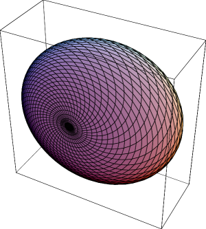
Figure 2. Stereographic projection from ${\mathbb{S}^{3}}-\{\text{north pole}\}$ to ${\mathbb{R}}^{3}$ of a spherical surface ${\mathbb{S}}_{\lambda}$ given by the union of all the geodesics of curvature $\lambda$ and length $\pi/\sqrt{1+\lambda^{2}}$ leaving from $p=(1,0,0,0)$.

In Section 5 of the paper we give the complete classification of complete, volume-preserving area-stationary surfaces in $({\mathbb{S}^{3}},g_{h})$ with non-empty singular set. In Theorem 5.3 we generalize the aforementioned Theorem E in [CHMY]: we prove that if $\Sigma$ is a $C^{2}$ complete, connected, immersed surface with constant mean curvature $H$ and at least an isolated singular point, then $\Sigma$ is congruent with the spherical surface $\mathcal{S}_{H}$ described as the union of all the geodesics of curvature $H$ and length $\pi/\sqrt{1+H^{2}}$ leaving from a given point, see Figure 2. Our main result in this section characterizes complete volume-preserving area-stationary surfaces with at least one singular curve $\Gamma$. The local description given in Theorem 4.3 of such a surface $\Sigma$ around $\Gamma$, and the orthogonality condition between singular curves and geodesics in Theorem 4.5, imply that a small neighborhood of $\Gamma$ in $\Sigma$ consists of the union of small pieces of all the geodesics $\gamma_{\varepsilon}$ of the same curvature leaving from $\Gamma$ orthogonally. By using the completeness of $\Sigma$ we can extend these geodesics until they meet another singular point. Finally, from a detailed study of the Jacobi vector field associated to the family $\gamma_{\varepsilon}$ we deduce that the singular curve $\Gamma$ must be a geodesic in $({\mathbb{S}^{3}},g_{h})$. This allows us to conclude that $\Sigma$ is congruent with one of the surfaces $\mathcal{C}_{\mu,\lambda}$ obtained when we leave orthogonally from a given geodesic of curvature $\mu$ by geodesics of curvature $\lambda$, see Example 5.8.

The classification of complete surfaces with empty singular set and constant mean curvature in $({\mathbb{S}^{3}},g_{h})$ seems to be a difficult problem. In Section 5 we prove some results in this direction. In Proposition 5.11 we show that the Clifford tori $\mathcal{T}_{\rho}$ are the only complete surfaces with constant mean curvature such that the Hopf vector field $V$ is always tangent to the surface. In Theorem 5.10 we characterize the Clifford tori as the unique compact embedded surfaces with empty singular set and constant mean curvature $H$ such that $H/\sqrt{1+H^{2}}$ is irrational. These results might suggest that Theorem 5.10 holds without any further assumption on the curvature $H$ of the surface.

In the last section of the paper we describe complete surfaces with constant mean curvature in $({\mathbb{S}^{3}},g_{h})$ which are invariant under the isometries of $({\mathbb{S}^{3}},g)$ fixing the vertical equator passing through $(1,0,0,0)$. For such a surface the equation of constant mean curvature can be reduced to a system of ordinary differential equations. Then, a detailed analysis of the solutions yields a counterpart in $({\mathbb{S}^{3}},g_{h})$ of the classification by C. Delaunay of rotationally invariant constant mean curvature surfaces in ${\mathbb{R}}^{3}$, later extended by W.-H. Hsiang [Hs] to $({\mathbb{S}^{3}},g)$. In particular we can find compact, embedded, unduloidal type surfaces with empty singular set and constant mean curvature $H$ such that $H/\sqrt{1+H^{2}}$ is rational. This provides an example illustrating that all the hypotheses in Theorem 5.10 are necessary.

In addition to the geometric interest of this work we believe that our results may be applied in two directions. First, they could be useful to solve the isoperimetric problem in $({\mathbb{S}^{3}},g_{h})$ which consists of enclosing a fixed amount of volume with the least possible boundary area. In fact, if we assume that the solutions to this problem are $C^{2}$ smooth and have at least one singular point, then they must coincide with one of the surfaces $\mathcal{S}_{\lambda}$ or $\mathcal{C}_{\mu,\lambda}$ introduced in Section 5. Second, our classification results could be utilized to find examples of constant mean curvature surfaces inside the Riemannian Berger spheres $({\mathbb{S}^{3}},g_{k})$. This is motivated by the fact that the metric space $({\mathbb{S}^{3}},d)$ associated to the Carnot-Carathéodory distance is limit, in the Gromov-Hausdorff sense, of the spaces $({\mathbb{S}^{3}},d_{k})$, where $d_{k}$ is the Riemannian distance of $g_{k}$ [Gr, p. 109].

The authors want to express their gratitude to O. Gil and M. Ritoré for encouraging them to write these notes and helping discussions. This work was initiated while A. Hurtado was visiting the University of Granada in the winter of 2006. The paper was finished during a short visit of C. Rosales to the University Jaume I (Castelló) in the summer of 2006.

2. Preliminaries

Throughout this paper we will identify a point $p=(x_{1},y_{1},x_{2},y_{2})\in{\mathbb{R}}^{4}$ with the quaternion $x_{1}+iy_{1}+jx_{2}+ky_{2}$. We denote the quaternion product and the scalar product of $p,q\in{\mathbb{R}}^{4}$ by $p\cdot q$ and $\big{<}p,q\big{>}$, respectively. The unit sphere ${\mathbb{S}^{3}}\subset{\mathbb{R}}^{4}$ endowed with the quaternion product is a compact, noncommutative, $3$-dimensional Lie group. For $p\in{\mathbb{S}^{3}}$, the right translation by $p$ is the diffeomorphism $R_{p}(q)=q\cdot p$. A basis of right invariant vector fields in $({\mathbb{S}^{3}},\cdot)$ given in terms of the Euclidean coordinate vector fields is

$$V(p): =i\cdot p=-y_{1}\,\frac{\partial}{\partial x_{1}}+x_{1}\,\frac{\partial}{\partial y_{1}}-y_{2}\,\frac{\partial}{\partial x_{2}}+x_{2}\,\frac{\partial}{\partial y_{2}},$$

$$E_{1}(p): =j\cdot p=-x_{2}\,\frac{\partial}{\partial x_{1}}+y_{2}\,\frac{\partial}{\partial y_{1}}+x_{1}\,\frac{\partial}{\partial x_{2}}-y_{1}\,\frac{\partial}{\partial y_{2}},$$

$$E_{2}(p): =k\cdot p=-y_{2}\,\frac{\partial}{\partial x_{1}}-x_{2}\,\frac{\partial}{\partial y_{1}}+y_{1}\,\frac{\partial}{\partial x_{2}}+x_{1}\,\frac{\partial}{\partial y_{2}}.$$

We define the horizontal distribution $\mathcal{H}$ in ${\mathbb{S}^{3}}$ as the smooth plane distribution generated by $E_{1}$ and $E_{2}$. The horizontal projection of a vector $X$ onto $\mathcal{H}$ is denoted by $X_{h}$. A vector field $X$ is horizontal if $X=X_{h}$. A horizontal curve is a piecewise $C^{1}$ curve such that the tangent vector (where defined) lies in the horizontal distribution.

We denote by $[X,Y]$ the Lie bracket of two $C^{1}$ tangent vector fields $X,Y$ on ${\mathbb{S}^{3}}$. Note that $[E_{1},V]=2E_{2}$, $[E_{2},V]=-2E_{1}$ and $[E_{1},E_{2}]=-2V$, so that $\mathcal{H}$ is a bracket generating distribution. Moreover, by Frobenius theorem we have that $\mathcal{H}$ is nonintegrable. The vector fields $E_{1}$ and $E_{2}$ generate the kernel of the contact $1$-form given by the restriction to the tangent bundle $T{\mathbb{S}^{3}}$ of $\omega:=-y_{1}\,dx_{1}+x_{1}\,dy_{1}-y_{2}\,dx_{2}+x_{2}\,dy_{2}$.

We introduce a sub-Riemannian metric $g_{h}$ on ${\mathbb{S}^{3}}$ by considering the Riemannian metric on $\mathcal{H}$ such that $\{E_{1},E_{2}\}$ is an orthonormal basis at every point. It is immediate that the Riemannian metric $g=\big{<}\cdot\,,\cdot\big{>}|_{{\mathbb{S}^{3}}}$ provides an extension to $T{\mathbb{S}^{3}}$ of the sub-Riemannian metric such that $\{E_{1},E_{2},V\}$ is orthonormal. The metric $g$ is bi-invariant and so the right translations $R_{p}$ and the left translations $L_{p}$ are isometries of $({\mathbb{S}^{3}},g)$. We denote by $D$ the Levi-Civitá connection on $({\mathbb{S}^{3}},g)$. The following derivatives can be easily computed

$$D_{E_{1}}E_{1} =0,\qquad\ \ \,\,D_{E_{2}}E_{2}=0,\qquad\quad\ \,D_{V}V=0,$$

(2.1) $$D_{E_{1}}E_{2} =-V,\qquad D_{E_{1}}V=E_{2},\qquad\,\ \,\,D_{E_{2}}V=-E_{1},$$

$$D_{E_{2}}E_{1} =V,\qquad\quad\!\!\,D_{V}E_{1}=-E_{2},\qquad\!D_{V}E_{2}=E_{1}.$$

For any tangent vector field $X$ on ${\mathbb{S}^{3}}$ we define $J(X):=D_{X}V$. Then we have $J(E_{1})=E_{2}$, $J(E_{2})=-E_{1}$ and $J(V)=0$, so that $J^{2}=-\text{Identity}$ when restricted to the horizontal distribution. It is also clear that

$$\big{<}J(X),Y\big{>}+\big{<}X,J(Y)\big{>}=0,$$

for any pair of vector fields $X$ and $Y$. The involution $J:\mathcal{H}\to\mathcal{H}$ together with the contact $1$-form $\omega=-y_{1}\,dx_{1}+x_{1}\,dy_{1}-y_{2}\,dx_{2}+x_{2}\,dy_{2}$ provides a pseudohermitian structure on ${\mathbb{S}^{3}}$, as stated in [CHMY, Appendix]. We remark that $J:\mathcal{H}\to\mathcal{H}$ coincides with the restriction to $\mathcal{H}$ of the complex structure on ${\mathbb{R}}^{4}$ given by the left multiplication by $i$, that is

$$J(X)=i\cdot X,\quad\text{ for any }X\in\mathcal{H}.$$

Now we introduce notions of volume and area in $({\mathbb{S}^{3}},g_{h})$. We will follow the same approach as in [RR] and [RR2]. The volume $V(\Omega)$ of a Borel set $\Omega\subseteq{\mathbb{S}^{3}}$ is the Haar measure associated to the quaternion product, which turns out to coincide with the Riemannian volume of $g$. Given a $C^{1}$ surface $\Sigma$ immersed in ${\mathbb{S}^{3}}$, and a unit vector field $N$ normal to $\Sigma$ in $({\mathbb{S}^{3}},g)$, we define the area of $\Sigma$ in $({\mathbb{S}^{3}},g_{h})$ by

(2.2) $$A(\Sigma):=\int_{\Sigma}|N_{h}|\,d\Sigma,$$

where $N_{h}=N-\big{<}N,V\big{>}\,V$, and $d\Sigma$ is the Riemannian area element on $\Sigma$. If $\Omega$ is an open set of ${\mathbb{S}^{3}}$ bounded by a $C^{2}$ surface $\Sigma$ then, as a consequence of the Riemannian divergence theorem, we have that $A(\Sigma)$ coincides with the sub-Riemannian perimeter of $\Omega$ defined by

$$\mathcal{P}(\Omega)=\sup\,\left\{\int_{\Omega}\operatorname{div}X\,dv;\,|X|\leqslant 1\right\},$$

where the supremum is taken over $C^{1}$ horizontal tangent vector fields on ${\mathbb{S}^{3}}$. In the definition above $dv$ and $\operatorname{div}$ are the Riemannian volume and divergence of $g$, respectively.

For a $C^{1}$ surface $\Sigma\subset{\mathbb{S}^{3}}$ the singular set $\Sigma_{0}$ consists of those points $p\in\Sigma$ for which the tangent plane $T_{p}\Sigma$ coincides with $\mathcal{H}_{p}$. As $\Sigma_{0}$ is closed and has empty interior in $\Sigma$, the regular set $\Sigma-\Sigma_{0}$ of $\Sigma$ is open and dense in $\Sigma$. It follows from the arguments in [De, Lemme 1], see also [Ba, Theorem 1.2], that for a $C^{2}$ surface $\Sigma$ the Hausdorff dimension of $\Sigma_{0}$ with respect to the Riemannian distance in ${\mathbb{S}^{3}}$ is less than two. If $\Sigma$ is oriented and $N$ is a unit normal vector to $\Sigma$ then we can describe the singular set as $\Sigma_{0}=\{p\in\Sigma:N_{h}(p)=0\}$. In the regular part $\Sigma-\Sigma_{0}$, we can define the horizontal Gauss map $\nu_{h}$ and the characteristic vector field $Z$, by

(2.3) $$\nu_{h}:=\frac{N_{h}}{|N_{h}|},\qquad Z:=J(\nu_{h})=i\cdot\nu_{h}.$$

As $Z$ is horizontal and orthogonal to $\nu_{h}$, we conclude that $Z$ is tangent to $\Sigma$. Hence $Z_{p}$ generates $T_{p}\Sigma\cap\mathcal{H}_{p}$. The integral curves of $Z$ in $\Sigma-\Sigma_{0}$ will be called characteristic curves of $\Sigma$. They are both tangent to $\Sigma$ and horizontal. Note that these curves depend on the unit normal $N$ to $\Sigma$. If we define

(2.4) $$S:=\big{<}N,V\big{>}\,\nu_{h}-|N_{h}|\,V,$$

then $\{Z_{p},S_{p}\}$ is an orthonormal basis of $T_{p}\Sigma$ whenever $p\in\Sigma-\Sigma_{0}$.

Any isometry of $({\mathbb{S}^{3}},g)$ leaving invariant the horizontal distribution preserves the area $A(\Sigma)$ of surfaces in $({\mathbb{S}^{3}},g_{h})$. Examples of such isometries are left and right translations. The rotation of angle $\theta$ given by

(2.5) $$r_{\theta}(x_{1},y_{1},x_{2},y_{2})=(x_{1},y_{1},(\cos\theta)x_{2}-(\sin\theta)y_{2},(\sin\theta)x_{2}+(\cos\theta)y_{2})$$

is also such an isometry since it transforms the orthonormal basis $\{E_{1},E_{2},V\}$ at $p$ into the orthonormal basis $\{(\cos\theta)E_{1}+(\sin\theta)E_{2},(-\sin\theta)E_{1}+(\cos\theta)E_{2},V\}$ at $r_{\theta}(p)$. We say that two surfaces $\Sigma_{1}$ and $\Sigma_{2}$ are congruent if there is an isometry $\phi$ of $({\mathbb{S}^{3}},g)$ preserving the horizontal distribution and such that $\phi(\Sigma_{1})=\Sigma_{2}$.

Finally we recall that the Hopf fibration $\mathcal{F}:{\mathbb{S}^{3}}\to{\mathbb{S}}^{2}\equiv{\mathbb{S}^{3}}\cap\{x_{1}=0\}$ is the Riemannian submersion given by $\mathcal{F}(p)=\overline{p}\cdot i\cdot p$ (here $\overline{p}$ denotes the conjugate of the quaternion $p$). In terms of Euclidean coordinates we get

$$\mathcal{F}(x_{1},y_{1},x_{2},y_{2})=(0,x^{2}_{1}+y^{2}_{1}-x_{2}^{2}-y_{2}^{2},2\,(x_{2}y_{1}-x_{1}y_{2}),2\,(x_{1}x_{2}+y_{1}y_{2})).$$

The fiber passing through $p\in{\mathbb{S}^{3}}$ is the great circle parameterized by $\exp(it)\cdot p$. Clearly the fibers are integral curves of the vertical vector $V$, which is sometimes known as the Hopf vector field. A lift of a curve $c:(-\varepsilon,\varepsilon)\to{\mathbb{S}}^{2}$ is a curve $\gamma:(-\varepsilon,\varepsilon)\to{\mathbb{S}^{3}}$ such that $\mathcal{F}(\gamma)=c$. By general properties of principal bundles we have that for any piecewise $C^{1}$ curve $c$ there is a unique horizontal lift of $c$ passing through a fixed point $p\in\mathcal{F}^{-1}(c(0))$, see [KN, p. 88]. For any $\rho\in(0,1)$ let $c_{\rho}$ be the geodesic circle of ${\mathbb{S}}^{2}$ contained in the plane $\{x_{1}=0,\,y_{1}=2\rho^{2}-1\}$. The set $\mathcal{T}_{\rho}=\mathcal{F}^{-1}(c_{\rho})$ is the Clifford torus in ${\mathbb{S}^{3}}$ described by the pairs of complex numbers $(z_{1},z_{2})$ such that $|z_{1}|^{2}=\rho^{2}$ and $|z_{2}|^{2}=1-\rho^{2}$.

3. Carnot-Carathéodory geodesics in ${\mathbb{S}^{3}}$

Let $\gamma:I\to{\mathbb{S}^{3}}$ be a piecewise $C^{1}$ curve defined on a compact interval $I\subset{\mathbb{R}}$. The length of $\gamma$ is the Riemannian length $L(\gamma):=\int_{I}|\dot{\gamma}|$. For any two points $p,q\in{\mathbb{S}^{3}}$ we can find, by Chow’s connectivity theorem [Gr, §1.2.B], a $C^{\infty}$ horizontal curve joining these points. The Carnot-Carathéodory distance $d(p,q)$ is defined as the infimum of the lengths of all piecewise $C^{1}$ horizontal curves joining $p$ and $q$. The topologies on ${\mathbb{S}^{3}}$ defined by $d$ and the Riemannian distance associated to $g$ are the same, see [Be, Cor. 2.6]. In the metric space $({\mathbb{S}^{3}},d)$ there is a natural extension for continuous curves of the notion of length, see [Be, p. 19]. We say that a continuous curve $\gamma$ joining $p$ and $q$ is length-minimizing if $L(\gamma)=d(p,q)$. Since the metric space $({\mathbb{S}^{3}},d)$ is complete we can apply the Hopf-Rinow theorem in sub-Riemannian geometry [Be, Thm. 2.7] to ensure the existence of length-minimizing curves joining two given points. Moreover, by [St, Cor. 6.2], see also [M, Chapter 5], any of these curves is $C^{\infty}$. In this section we are interested in smooth curves which are critical points of length under any variation by horizontal curves with fixed endpoints. These curves are sometimes known as Carnot-Carathéodory geodesics and they have been extensively studied in general sub-Riemannian manifolds, see [M]. By the aforementioned regularity result any length-minimizing curve in $({\mathbb{S}^{3}},d)$ is a geodesic. In this section we follow the approach in [RR2, § 3] to obtain a variational characterization of the geodesics.

Let $\gamma:I\to{\mathbb{S}^{3}}$ be a $C^{2}$ horizontal curve. A smooth variation of $\gamma$ is a $C^{2}$ map $F:I\times J\to{\mathbb{S}^{3}}$, where $J$ is an open interval around the origin, such that $F(s,0)=\gamma(s)$. We denote $\gamma_{\varepsilon}(s)=F(s,\varepsilon)$. Let $X_{\varepsilon}(s)$ be the vector field along $\gamma_{\varepsilon}$ given by $(\partial F/\partial\varepsilon)(s,\varepsilon)$. Trivially $[X_{\varepsilon},\dot{\gamma}_{\varepsilon}]=0$. Let $X=X_{0}$. We say that the variation is admissible if the curves $\gamma_{\varepsilon}$ are horizontal and have fixed extreme points. For such a variation the vector field $X$ vanishes at the endpoints of $\gamma$ and satisfies

$$0=\dot{\gamma}\big{(}\big{<}X,V\big{>}\big{)}-2\,\big{<}X_{h},J(\dot{\gamma})\big{>}.$$

The equation above characterizes the vector fields along $\gamma$ associated to admissible variations. By using the first variation of length in Riemannian geometry we can prove the following result, see [RR2, Proposition 3.1] for details.

Proposition 3.1.

Let $\gamma:I\to{\mathbb{S}^{3}}$ be a $C^{2}$ horizontal curve parameterized by arc-length. Then $\gamma$ is a critical point of length for any admissible variation if and only if there is $\lambda\in{\mathbb{R}}$ such that $\gamma$ satisfies the second order ordinary differential equation

(3.1) $$D_{\dot{\gamma}}\dot{\gamma}+2\lambda\,J(\dot{\gamma})=0.$$

We will say that a $C^{2}$ horizontal curve $\gamma$ is a geodesic of curvature $\lambda$ in $({\mathbb{S}^{3}},g_{h})$ if $\gamma$ is parameterized by arc-length and satisfies equation (3.1). Observe that the parameter $\lambda$ in (3.1) changes to $-\lambda$ for the reversed curve $\gamma(-s)$, while it is preserved for the antipodal curve $-\gamma(s)$. In general, any isometry of $({\mathbb{S}^{3}},g)$ preserving the horizontal distribution transforms geodesics in geodesics since it respects the connection $D$ of $g$ and commutes with $J$.

Given a point $p\in{\mathbb{S}^{3}}$, a unit horizontal vector $v\in T_{p}{\mathbb{S}^{3}}$, and $\lambda\in{\mathbb{R}}$, we denote by $\gamma_{p,v}^{\lambda}$ the unique solution to (3.1) with initial conditions $\gamma(0)=p$ and $\dot{\gamma}(0)=v$. The curve $\gamma_{p,v}^{\lambda}$ is a geodesic since it is horizontal and parameterized by arc-length (the functions $\big{<}\dot{\gamma},V\big{>}$ and $|\dot{\gamma}|^{2}$ are constant along any solution of (3.1)). Clearly for any right translation $R_{q}$ we have $R_{q}(\gamma^{\lambda}_{p,v})=\gamma^{\lambda}_{p\cdot q,v\cdot q}$.

Now we compute the geodesics in Euclidean coordinates. Consider a $C^{2}$ smooth curve $\gamma=(x_{1},y_{1},x_{2},y_{2})\in{\mathbb{S}^{3}}$ parameterized by arc-length $s$. We denote $\ddot{\gamma}=(\ddot{x}_{1},\ddot{y}_{1},\ddot{x}_{2},\ddot{y}_{2})$. The tangent and normal projections of $\ddot{\gamma}$ onto $T{\mathbb{S}^{3}}$ and $(T{\mathbb{S}^{3}})^{\bot}$ are given respectively by $D_{\dot{\gamma}}\dot{\gamma}$ and $\text{II}(\dot{\gamma},\dot{\gamma})\,\eta$, where II is the second fundamental form of ${\mathbb{S}^{3}}$ in ${\mathbb{R}}^{4}$ with respect to the unit normal vector $\eta(p)=p$. Hence we obtain

(3.2) $$\ddot{\gamma}=D_{\dot{\gamma}}\dot{\gamma}-\gamma.$$

As a consequence equation (3.1) reads

$$\ddot{\gamma}+\gamma+2\lambda\,(i\cdot\dot{\gamma})=0.$$

If we denote $z_{n}=x_{n}+iy_{n}$ then the previous equation is equivalent to

$$\ddot{z}_{n}+z_{n}+2\lambda i\,\dot{z}_{n}=0,\qquad n=1,2.$$

Therefore, an explicit integration gives for $n=1,2$

(3.3) $$z_{n}(s)=C_{1n}\,\exp\{(-\lambda+\sqrt{1+\lambda^{2}})\,is\}+C_{2n}\,\exp\{-(\lambda+\sqrt{1+\lambda^{2}})\,is\},$$

where $C_{1n}$ and $C_{2n}$ are complex constants. Thus, if we denote $C^{r}_{mn}=\text{Re}(C_{mn})$ and $C^{i}_{mn}=\text{Im}(C_{mn})$ then we have

$$x_{n}(s) =(C^{r}_{1n}+C^{r}_{2n})\,\cos(\lambda s)\,\cos(\sqrt{1+\lambda^{2}}\,s)+(C^{r}_{1n}-C^{r}_{2n})\,\sin(\lambda s)\,\sin(\sqrt{1+\lambda^{2}}\,s)$$

$$+(C^{i}_{1n}+C^{i}_{2n})\,\sin(\lambda s)\,\cos(\sqrt{1+\lambda^{2}}\,s)+(C^{i}_{2n}-C^{i}_{1n})\,\cos(\lambda s)\,\sin(\sqrt{1+\lambda^{2}}\,s),$$

$$y_{n}(s) =(C^{i}_{1n}+C^{i}_{2n})\,\cos(\lambda s)\,\cos(\sqrt{1+\lambda^{2}}\,s)-(C^{i}_{2n}-C^{i}_{1n})\,\sin(\lambda s)\,\sin(\sqrt{1+\lambda^{2}}\,s)$$

$$-(C^{r}_{1n}+C^{r}_{2n})\,\sin(\lambda s)\,\cos(\sqrt{1+\lambda^{2}}\,s)+(C^{r}_{1n}-C^{r}_{2n})\,\cos(\lambda s)\,\sin(\sqrt{1+\lambda^{2}}\,s).$$

Suppose that $\gamma(0)=(x_{1}^{0},y_{1}^{0},x_{2}^{0},y_{2}^{0})$ and $\dot{\gamma}(0)=(u_{1}^{0},w_{1}^{0},u_{2}^{0},w_{2}^{0})$. It is easy to see from (3.3) that

$$C^{r}_{1n}+C^{r}_{2n} =x^{0}_{n},\qquad C^{r}_{1n}-C^{r}_{2n}=\frac{w^{0}_{n}+\lambda x^{0}_{n}}{\sqrt{1+\lambda^{2}}},$$

$$C^{i}_{1n}+C^{i}_{2n} =y^{0}_{n},\qquad\,C^{i}_{2n}-C^{i}_{1n}=\frac{u^{0}_{n}-\lambda y^{0}_{n}}{\sqrt{1+\lambda^{2}}}.$$

So, by substituting the previous equalities in the expressions of $x_{n}(s)$ and $y_{n}(s)$ we obtain

(3.4) $$x_{n}(s) =x^{0}_{n}\,\cos(\lambda s)\,\cos(\sqrt{1+\lambda^{2}}\,s)+\frac{w^{0}_{n}+\lambda x^{0}_{n}}{\sqrt{1+\lambda^{2}}}\,\sin(\lambda s)\,\sin(\sqrt{1+\lambda^{2}}\,s)$$

$$+y^{0}_{n}\,\sin(\lambda s)\,\cos(\sqrt{1+\lambda^{2}}\,s)+\frac{u^{0}_{n}-\lambda y^{0}_{n}}{\sqrt{1+\lambda^{2}}}\,\cos(\lambda s)\,\sin(\sqrt{1+\lambda^{2}}\,s).$$

$$y_{n}(s) =y^{0}_{n}\,\cos(\lambda s)\,\cos(\sqrt{1+\lambda^{2}}\,s)-\frac{u^{0}_{n}-\lambda y^{0}_{n}}{\sqrt{1+\lambda^{2}}}\,\sin(\lambda s)\,\sin(\sqrt{1+\lambda^{2}}\,s)$$

$$-x^{0}_{n}\,\sin(\lambda s)\,\cos(\sqrt{1+\lambda^{2}}\,s)+\frac{w^{0}_{n}+\lambda x^{0}_{n}}{\sqrt{1+\lambda^{2}}}\,\cos(\lambda s)\,\sin(\sqrt{1+\lambda^{2}}\,s).$$

We conclude that the geodesic $\gamma^{\lambda}_{p,v}$ is given for any $s\in{\mathbb{R}}$ by

(3.5) $$\gamma^{\lambda}_{p,v}(s) =\cos(\lambda s)\,\cos(\sqrt{1+\lambda^{2}}\,s)\,p+\frac{\sin(\lambda s)\,\sin(\sqrt{1+\lambda^{2}}\,s)}{\sqrt{1+\lambda^{2}}}\,(\lambda p-J(v))$$

$$-\sin(\lambda s)\,\cos(\sqrt{1+\lambda^{2}}\,s)\,V(p)+\frac{\cos(\lambda s)\,\sin(\sqrt{1+\lambda^{2}}\,s)}{\sqrt{1+\lambda^{2}}}\,(\lambda V(p)+v).$$

In particular, for $\lambda=0$ we get

$$\gamma^{0}_{p,v}(s)=\cos(s)\,p+\sin(s)\,v,$$

which is a horizontal great circle of ${\mathbb{S}^{3}}$. This was already observed in [CHMY, Lemma 7.1].

Now we prove a characterization of the geodesics that will be useful in Section 5. The result also shows that the geodesics are horizontal lifts via the Hopf fibration $\mathcal{F}:{\mathbb{S}^{3}}\to{\mathbb{S}}^{2}$ of the geodesic circles in ${\mathbb{S}}^{2}$, see [M, Thm. 1.26] for a general statement for principal bundles.

Lemma 3.2.

Let $\gamma:I\to{\mathbb{S}^{3}}$ be a $C^{2}$ horizontal curve parameterized by arc-length. The following assertions are equivalent

• $\gamma$ is a geodesic of curvature $\lambda$ in $({\mathbb{S}^{3}},g_{h})$,

• $\big{<}\ddot{\gamma},J(\dot{\gamma})\big{>}=-2\lambda$,

• the Hopf fibration $\mathcal{F}(\gamma)$ is a piece of a geodesic circle in ${\mathbb{S}}^{2}$ with constant geodesic curvature $\lambda$ in ${\mathbb{S}}^{2}$.

Proof.

As $\gamma$ is horizontal and parameterized by arc-length we have

$$0 =\dot{\gamma}\,(\big{<}\dot{\gamma},\dot{\gamma}\big{>})=2\,\big{<}D_{\dot{\gamma}}\dot{\gamma},\dot{\gamma}\big{>},$$

$$0 =\dot{\gamma}\,(\big{<}\dot{\gamma},V(\gamma)\big{>})=\big{<}D_{\dot{\gamma}}\dot{\gamma},V(\gamma)\big{>}+\big{<}\dot{\gamma},J(\dot{\gamma})\big{>}=\big{<}D_{\dot{\gamma}}\dot{\gamma},V(\gamma)\big{>}.$$

As $\{\dot{\gamma},J(\dot{\gamma}),V(\gamma)\}$ is an orthonormal basis of $T{\mathbb{S}^{3}}$ along $\gamma$, we deduce that $D_{\dot{\gamma}}\dot{\gamma}$ is proportional to $J(\dot{\gamma})$ at any point of $\gamma$. On the other hand from (3.2) we have

$$\big{<}D_{\dot{\gamma}}\dot{\gamma},J(\dot{\gamma})\big{>}=\big{<}\ddot{\gamma}+\gamma,J(\dot{\gamma})\big{>}=\big{<}\ddot{\gamma},J(\dot{\gamma})\big{>},$$

where in the second equality we have used that the position vector field $\eta(p)=p$ in ${\mathbb{R}}^{4}$ provides a unit normal to ${\mathbb{S}^{3}}$. This proves that (i) and (ii) are equivalent.

Let us see that (i) is equivalent to (iii). Note that $\mathcal{F}(R_{q}(p))=(L_{\overline{q}}\circ R_{q})(\mathcal{F}(p))$ for any $p,q\in{\mathbb{S}^{3}}$. Hence we only have to prove the claim for a geodesic $\gamma$ leaving from $p=(1,0,0,0)$. Let $v=(\cos\theta)\,E_{1}(p)+(\sin\theta)\,E_{2}(p)$ be the initial velocity of such a geodesic. A direct computation from (3.4) shows that the Euclidean coordinates $(y_{1},x_{2},y_{2})$ of the curve $c=\mathcal{F}(\gamma)$ are given by

$$y_{1}(s) =1-\frac{2}{1+\lambda^{2}}\,\sin^{2}(\sqrt{1+\lambda^{2}}\,s),$$

$$x_{2}(s) =\frac{-\sin(2\sqrt{1+\lambda^{2}}\,s)}{\sqrt{1+\lambda^{2}}}\,\sin\theta+\frac{2\lambda\,\sin^{2}(\sqrt{1+\lambda^{2}}\,s)}{1+\lambda^{2}}\,\cos\theta.$$

$$y_{2}(s) =\frac{\sin(2\sqrt{1+\lambda^{2}}\,s)}{\sqrt{1+\lambda^{2}}}\,\cos\theta+\frac{2\lambda\,\sin^{2}(\sqrt{1+\lambda^{2}}\,s)}{1+\lambda^{2}}\,\sin\theta.$$

From the equations above it is not difficult to check that the binormal vector to $c$ in ${\mathbb{R}}^{3}$ is $|\dot{c}\wedge\ddot{c}|^{-1}(\dot{c}\wedge\ddot{c})(s)=(1+\lambda^{2})^{-1/2}\,(\lambda,\sin\theta,\cos\theta)$. It follows that the curve $c$ lies inside a Euclidean plane and so, it must be a piece of a geodesic circle in ${\mathbb{S}}^{2}$. Moreover, the geodesic curvature of $c$ in ${\mathbb{S}}^{2}$ with respect to the unit normal vector given by $|c\wedge\dot{c}|^{-1}\,(c\wedge\dot{c})$ equals $\lambda$. This proves that (i) implies (iii). Conversely, let us suppose that $c=\mathcal{F}(\gamma)$ is a piece of a geodesic circle of curvature $\lambda$ in ${\mathbb{S}}^{2}$. We consider the geodesic $\gamma^{\lambda}_{p,v}$ in $({\mathbb{S}^{3}},g_{h})$ with initial conditions $p=\gamma(0)$ and $v=\dot{\gamma}(0)$. The previous arguments and the uniqueness of constant geodesic curvature curves in ${\mathbb{S}}^{2}$ for given initial conditions imply that $\mathcal{F}(\gamma^{\lambda}_{p,v})=c$. By using the uniqueness of the horizontal lifts of a curve we conclude that $\gamma=\gamma^{\lambda}_{p,v}$. ∎

In the next result we show that the topological behaviour of a geodesic in $({\mathbb{S}^{3}},g_{h})$ depends on the curvature of the geodesic. Recall that $\mathcal{T}_{\rho}$ denotes the Clifford torus consisting of the pairs $(z_{1},z_{2})\in{\mathbb{S}^{3}}$ such that $|z_{1}|^{2}=\rho^{2}$.

Proposition 3.3.

Let $\gamma:{\mathbb{R}}\to{\mathbb{S}^{3}}$ be a complete geodesic of curvature $\lambda$. Then $\gamma$ is a closed curve diffeomorphic to a circle if and only if $\lambda/\sqrt{1+\lambda^{2}}$ is a rational number. Otherwise $\gamma$ is diffeomorphic to a straight line and there is a right translation $R_{q}$ such that $R_{q}(\gamma)$ is a dense subset inside a Clifford torus $\mathcal{T}_{\rho}$.

Proof.

In order to characterize when $\gamma$ is a closed curve diffeomorphic to a circle it would be enough to analyze the equality $\gamma(s_{1})=\gamma(s_{2})$ from (3.5). However we will prove the proposition by using the description of a geodesic contained inside a Clifford torus $\mathcal{T}_{\rho}$.

We shall use complex notation for the points in ${\mathbb{S}^{3}}$. Let $q=(z_{1},z_{2})\in\mathcal{T}_{\rho}$. It is easy to check that there are only two unit horizontal vectors in $T_{q}\mathcal{T}_{\rho}$. These are $w=i\cdot(\alpha z_{1},-\alpha^{-1}z_{2})$ and $-w$, where $\alpha=\rho^{-1}\sqrt{1-\rho^{2}}$. Take the geodesic $\gamma^{\lambda}_{q,w}=(z_{1}(s),z_{2}(s))$ of curvature $\lambda$. A direct computation from (3.4) gives us

$$|z_{1}(s)|^{2}=\rho^{2}\left(\cos^{2}(\sqrt{1+\lambda^{2}}\,s)+\frac{(\lambda+\alpha)^{2}}{1+\lambda^{2}}\,\sin^{2}(\sqrt{1+\lambda^{2}}\,s)\right),$$

so that $\gamma^{\lambda}_{q,w}$ is entirely contained in $\mathcal{T}_{\rho}$ if and only if $\lambda=(2\rho^{2}-1)/(2\rho\sqrt{1-\rho^{2}})$. Consider the map $\varphi(x,y)=(\rho\,\exp(2\pi ix),\sqrt{1-\rho^{2}}\,\exp(2\pi iy))$, which is a diffeomorphism between the flat torus ${\mathbb{R}}^{2}/\mathbb{Z}^{2}$ and $\mathcal{T}_{\rho}$ . If we choose the curvature $\lambda$ as above and we put $q=\varphi(\theta,\theta^{\prime})$ then we deduce from (3.4) that

$$\gamma^{\lambda}_{q,w}(s)=\varphi\left(\frac{(\sqrt{1+\lambda^{2}}-\lambda)\,s}{2\pi}+\theta,\frac{-(\lambda+\sqrt{1+\lambda^{2}})\,s}{2\pi}+\theta^{\prime}\right).$$

This implies that $\gamma^{\lambda}_{q,w}$ is a reparameterization of $\varphi(r(t))$, where $r(t)=mt+n$ is a straight line in ${\mathbb{R}}^{2}/\mathbb{Z}^{2}$ with slope

$$m=\frac{\lambda+\sqrt{1+\lambda^{2}}}{\lambda-\sqrt{1+\lambda^{2}}}=\frac{(\lambda/\sqrt{1+\lambda^{2}})+1}{(\lambda/\sqrt{1+\lambda^{2}})-1}.$$

As a consequence $\gamma^{\lambda}_{q,w}$ is a closed curve diffeomorphic to a circle if and only if $\lambda/\sqrt{1+\lambda^{2}}$ is a rational number. Otherwise $\gamma^{\lambda}_{q,w}$ is a dense curve in $\mathcal{T}_{\rho}$ diffeomorphic to a straight line.

Finally, let us consider any complete geodesic $\gamma=\gamma^{\lambda}_{p,v}$ in $({\mathbb{S}^{3}},g_{h})$. After applying a right translation we can suppose that $p=(1,0)$ and $v=(0,\exp(i\theta))$. Let $\rho\in(0,1)$ so that $\lambda/\sqrt{1+\lambda^{2}}=2\rho^{2}-1$. Take the point $q=(\rho,\sqrt{1-\rho^{2}}\,i\exp(i\theta))\in\mathcal{T}_{\rho}$. It is easy to check that the vector $v\cdot q$ coincides with the unit horizontal vector $w\in T_{q}\mathcal{T}_{\rho}$ such that $\gamma^{\lambda}_{q,w}\subset\mathcal{T}_{\rho}$. The proof of the proposition then follows by using that $R_{q}(\gamma^{\lambda}_{p,v})=\gamma^{\lambda}_{q,w}$ and the properties previously shown for geodesics inside $\mathcal{T}_{\rho}$. ∎

Figure 1. Stereographic projection from ${\mathbb{S}^{3}}-\{\text{north pole}\}$ to ${\mathbb{R}}^{3}$ of a sub-Riemannian geodesic which is dense inside a Clifford torus.

We finish this section with some analytical properties for the vector field associated to a variation of a curve which is a geodesic. The proofs use the same arguments as in Lemma 3.5 and Lemma 3.6 in [RR2].

Lemma 3.4.

Let $\gamma:I\to{\mathbb{S}^{3}}$ be a geodesic of curvature $\lambda$. Suppose that $X$ is the $C^{1}$ vector field associated to a variation of $\gamma$ by horizontal curves $\gamma_{\varepsilon}$ parameterized by arc-length. Then we have

• The function $\lambda\,\big{<}X,V(\gamma)\big{>}+\big{<}X,\dot{\gamma}\big{>}$ is constant along $\gamma$.

• If any $\gamma_{\varepsilon}$ is a geodesic of curvature $\lambda$ and $X$ is $C^{2}$ smooth, then $X$ satisfies the second order differential equation $D_{\dot{\gamma}}D_{\dot{\gamma}}{X}+R(X,\dot{\gamma})\dot{\gamma}+2\lambda\,(J(D_{\dot{\gamma}}{X})-\big{<}X,\dot{\gamma}\big{>}\,V(\gamma))=0$, where $R$ denotes the Riemannian curvature tensor in $({\mathbb{S}^{3}},g)$.

The linear differential equation in Lemma 3.4 (ii) is the Jacobi equation for geodesics of curvature $\lambda$ in $({\mathbb{S}^{3}},g_{h})$. We will call any solution of this equation a Jacobi field along $\gamma$.

4. Area-stationary surfaces with or without a volume constraint

In this section we introduce and characterize critical surfaces for the area functional (2.2) with or without a volume constraint. We also state without proof some properties for such surfaces that will be useful in order to obtain classifications results. For a detailed development we refer the reader to [RR2, §4] and the references therein.

Let $\Sigma\subset{\mathbb{S}^{3}}$ be an oriented immersed surface of class $C^{2}$. Consider a $C^{1}$ vector field $X$ with compact support on $\Sigma$ and tangent to ${\mathbb{S}^{3}}$. For $t$ small we denote $\Sigma_{t}=\{\exp_{p}(tX_{p});p\in\Sigma\}$, which is an immersed surface. Here $\exp_{p}$ is the exponential map of $({\mathbb{S}^{3}},g)$ at the point $p$. The family $\{\Sigma_{t}\}$, for $t$ small, is the variation of $\Sigma$ induced by $X$. Note that we allow the variations to move the singular set $\Sigma_{0}$ of $\Sigma$. Define $A(t):=A(\Sigma_{t})$. If $\Sigma$ is the boundary of a region $\Omega\subset{\mathbb{S}^{3}}$ then we can consider a $C^{1}$ family of regions $\Omega_{t}$ such that $\Omega_{0}=\Omega$ and $\partial\Omega_{t}=\Sigma_{t}$. We define $V(t):=V(\Omega_{t})$. We say that the variation induced by $X$ is volume-preserving if $V(t)$ is constant for any $t$ small enough. We say that $\Sigma$ is area-stationary if $A^{\prime}(0)=0$ for any variation of $\Sigma$. In case that $\Sigma$ encloses a region $\Omega$, we say that $\Sigma$ is area-stationary under a volume constraint or volume-preserving area-stationary if $A^{\prime}(0)=0$ for any volume-preserving variation of $\Sigma$.

Suppose that $\Omega$ is the region bounded by a $C^{2}$ embedded compact surface $\Sigma$. We shall always choose the unit normal $N$ to $\Sigma$ in $({\mathbb{S}^{3}},g)$ pointing into $\Omega$. The computation of $V^{\prime}(0)$ is well known, and it is given by ([Si, §9])

(4.1) $$V^{\prime}(0)=\int_{\Omega}\operatorname{div}X\,dv=-\int_{\Sigma}u\,d\Sigma,$$

where $u=\big{<}X,N\big{>}$. It follows that $u$ has mean zero whenever the variation is volume-preserving. Conversely, it was proved in [BdCE, Lemma 2.2] that, given a $C^{1}$ function $u:\Sigma\to{\mathbb{R}}$ with mean zero, we can construct a volume-preserving variation of $\Omega$ so that the normal component of $X$ equals $u$.

Remark 4.1.

For a compact immersed $C^{2}$ surface $\Sigma$ in ${\mathbb{S}^{3}}$ there is a notion of volume enclosed by $\Sigma$. The first variation for this volume functional is given by (4.1). We refer the reader to [BdCE, p. 125] for details.

Now assume that the divergence relative to $\Sigma$ of the horizontal Gauss map $\nu_{h}$ defined in (2.3) satisfies $\operatorname{div}_{\Sigma}\nu_{h}\in L^{1}(\Sigma)$. In this case the first variation of the area functional $A(t)$ can be obtained as in [RR2, Lemma 4.3]. We get

(4.2) $$A^{\prime}(0)=\int_{\Sigma}u\,\big{(}\operatorname{div}_{\Sigma}\nu_{h}\big{)}\,d\Sigma-\int_{\Sigma}\operatorname{div}_{\Sigma}\big{(}u\,(\nu_{h})^{\top}\big{)}\,d\Sigma,$$

where $(\nu_{h})^{\top}$ is the projection of $\nu_{h}$ onto the tangent space to $\Sigma$.

Let $\Sigma$ be a $C^{2}$ immersed surface in ${\mathbb{S}^{3}}$ with a $C^{1}$ unit normal vector $N$. Outside the singular set $\Sigma_{0}$ of $\Sigma$ we define the mean curvature $H$ in $({\mathbb{S}^{3}},g_{h})$ by the equality

(4.3) $$-2H(p):=(\operatorname{div}_{\Sigma}\nu_{h})(p),\qquad p\in\Sigma-\Sigma_{0}.$$

This notion of mean curvature agrees with the ones introduced in [CHMY] and [HP]. We say that $\Sigma$ is a minimal surface if $H\equiv 0$ on $\Sigma-\Sigma_{0}$. By using variations supported in $\Sigma-\Sigma_{0}$, the first variation of area (4.2), and the first variation of volume (4.1), we deduce that the mean curvature of $\Sigma-\Sigma_{0}$ is respectively zero or constant if $\Sigma$ is area-stationary or volume-preserving area-stationary. In $\Sigma-\Sigma_{0}$ we can consider the orthonormal basis $\{Z,S\}$ defined in (2.3) and (2.4), so that we get from (4.3)

$$-2H=\big{<}D_{Z}\nu_{h},Z\big{>}+\big{<}D_{S}\nu_{h},S\big{>}.$$

It is easy to check ([RR2, Lemma 4.2]) that for any tangent vector $X$ to $\Sigma$ we have

$$D_{X}\nu_{h}=|N_{h}|^{-1}\,\big{(}\big{<}D_{X}N,Z\big{>}+\big{<}N,V\big{>}\,\big{<}X,\nu_{h}\big{>}\big{)}\,Z+\big{<}Z,X\big{>}\,V.$$

In particular by taking $X=Z$ and $X=S$ we deduce the following expression for the mean curvature

(4.4) $$2H=|N_{h}|^{-1}\,\text{II}(Z,Z),$$

where II is the second fundamental form of $\Sigma$ with respect to $N$ in $({\mathbb{S}^{3}},g)$.

On the other hand, by the arguments in [RR2, Thm. 4.8], any characteristic curve $\gamma$ of a $C^{2}$ immersed surface $\Sigma$ satisfies

(4.5) $$D_{\dot{\gamma}}\dot{\gamma}=-2H\,J(\dot{\gamma}).$$

From the previous equality we deduce that $\Sigma-\Sigma_{0}$ is a ruled surface in $({\mathbb{S}^{3}},g_{h})$ whenever $H$ is constant, see also [HP, Cor. 6.10].

Theorem 4.2.

Let $\Sigma$ be an oriented $C^{2}$ immersed surface in $({\mathbb{S}^{3}},g_{h})$ with constant mean curvature $H$ outside the singular set. Then any characteristic curve of $\Sigma$ is an open arc of a geodesic of curvature $H$ in $({\mathbb{S}^{3}},g_{h})$.

Now we describe the configuration of the singular set $\Sigma_{0}$ of a constant mean curvature surface $\Sigma$ in $({\mathbb{S}^{3}},g_{h})$. The set $\Sigma_{0}$ was studied by J.-H. Cheng, J.-F. Hwang, A. Malchiodi and P. Yang [CHMY] for surfaces with bounded mean curvature inside the first Heisenberg group. As indicated by the authors in [CHMY, Lemma 7.3] and [CHMY, Proof of Thm. E], their local arguments also apply for spherical pseudohermitian $3$-manifolds. We gather their results in the following theorem.

Theorem 4.3 ([CHMY, Theorem B]).

Let $\Sigma$ be a $C^{2}$ oriented immersed surface in $({\mathbb{S}^{3}},g_{h})$ with constant mean curvature $H$ off of the singular set $\Sigma_{0}$. Then $\Sigma_{0}$ consists of isolated points and $C^{1}$ curves with non-vanishing tangent vector. Moreover, we have

• $($[CHMY, Thm. 3.10]$)$ If $p\in\Sigma_{0}$ is isolated then there exists $r>0$ and $\lambda\in{\mathbb{R}}$ with $|\lambda|=|H|$ such that the set described as

  $$D_{r}(p)=\{\gamma_{p,v}^{\lambda}(s);v\in T_{p}\Sigma,\,|v|=1,\,s\in[0,r)\},$$

  is an open neighborhood of $p$ in $\Sigma$.

• $($[CHMY, Prop. 3.5 and Cor. 3.6]$)$ If $p$ is contained in a $C^{1}$ curve $\Gamma\subset\Sigma_{0}$ then there is a neighborhood $B$ of $p$ in $\Sigma$ such that $B\cap\Gamma$ is a connected curve and $B-\Gamma$ is the union of two disjoint connected open sets $B^{+}$ and $B^{-}$ contained in $\Sigma-\Sigma_{0}$. Furthermore, for any $q\in\Gamma\cap B$ there are exactly two geodesics $\gamma_{1}^{\lambda}\subset B^{+}$ and $\gamma_{2}^{\lambda}\subset B^{-}$ starting from $q$ and meeting transversally $\Gamma$ at $q$ with opposite initial velocities. The curvature $\lambda$ does not depend on $q\in\Gamma\cap B$ and satisfies $|\lambda|=|H|$.

Remark 4.4.

The relation between $\lambda$ and $H$ depends on the value of the normal $N$ to $\Sigma$ in the singular point $p$. If $N_{p}=V_{p}$ then $\lambda=H$, whereas $\lambda=-H$ when $N_{p}=-V_{p}$. In case $\lambda=H$ the geodesics $\gamma^{\lambda}$ in Theorem 4.3 are characteristic curves of $\Sigma$.

The characterization of area-stationary surfaces with or without a volume constraint in $({\mathbb{S}^{3}},g_{h})$ is similar to the one obtained by M. Ritoré and the second author in [RR2, Thm. 4.16]. We can also improve, as in [RR2, Prop. 4.19], the $C^{1}$ regularity of the singular curves of an area-stationary surface.

Theorem 4.5.

Let $\Sigma$ be an oriented $C^{2}$ immersed surface in ${\mathbb{S}^{3}}$. The followings assertions are equivalent

• $\Sigma$ is area-stationary $($resp. volume-preserving area-stationary$)$ in $({\mathbb{S}^{3}},g_{h})$.

• The mean curvature of $\Sigma-\Sigma_{0}$ is zero $($resp. constant$)$ and the characteristic curves meet orthogonally the singular curves when they exist.

Moreover, if $(\emph{i})$ holds then the singular curves of $\Sigma$ are $C^{2}$ smooth.

Example 4.6.

1. Every totally geodesic $2$-sphere in $({\mathbb{S}^{3}},g)$ is a compact minimal surface in $({\mathbb{S}^{3}},g_{h})$. In fact, for any $q\in{\mathbb{S}^{3}}$, the $2$-sphere ${\mathbb{S}^{3}}\cap q^{\bot}$ is the union of all the points $\gamma^{0}_{p,v}(s)$ where $p=-i\cdot q$, the unit vector $v\in T_{p}{\mathbb{S}^{3}}$ is horizontal, and $s\in[0,\pi]$. These spheres have two singular points at $p$ and $-p$. In particular they are area-stationary surfaces by Theorem 4.5.

2. For any $\rho\in(0,1)$ the Clifford torus $\mathcal{T}_{\rho}$ has no singular points since the vertical vector $V$ is tangent to this surface. We consider the unit normal vector to $\mathcal{T}_{\rho}$ in $({\mathbb{S}^{3}},g)$ given for $q=(z_{1},z_{2})$ by $N(q)=(\alpha z_{1},-\alpha^{-1}z_{2})$, where $\alpha=\rho^{-1}\,\sqrt{1-\rho^{2}}$. As $\big{<}N,V\big{>}=0$ then we have $N=N_{h}=\nu_{h}$ and so $Z=J(N)$. Let $\lambda=(2\rho^{2}-1)/(2\rho\sqrt{1-\rho^{2}})$. It was shown in the proof of Proposition 3.3 that the geodesic $\gamma^{\lambda}_{q,w}$ with $w=Z(q)$ is entirely contained in $\mathcal{T}_{\rho}$. The tangent vector to this geodesic equals $Z$ since the singular set is empty. We conclude that $\gamma^{\lambda}_{q,w}$ is a characteristic curve of $\mathcal{T}_{\rho}$. By using (4.5) we deduce that $\mathcal{T}_{\rho}$ has constant mean curvature $H=(2\rho^{2}-1)/(2\rho\sqrt{1-\rho^{2}})$ with respect to the normal $N$. By Theorem 4.5 the surface $\mathcal{T}_{\rho}$ is volume-preserving area-stationary for any $\rho\in(0,1)$. Moreover, $\mathcal{T}_{\rho}$ is area-stationary for $\rho=\sqrt{2}/2$.

The previous examples were found in [CHMY]. In [CHMY, Theorem E], J.- H. Cheng, J.-F. Hwang, A. Malchiodi and P. Yang described the possible topological types for a compact surface with bounded mean curvature inside a spherical pseudohermitian $3$-manifold were. More precisely, they proved the following result.

Theorem 4.7.

Let $\Sigma$ be an immersed $C^{2}$ compact, connected, oriented surface in $({\mathbb{S}^{3}},g_{h})$ with bounded mean curvature outside the singular set. If $\Sigma$ contains an isolated singular point then $\Sigma$ is homeomorphic to a sphere. Otherwise $\Sigma$ is homeomorphic to a torus.

5. Classification results for complete stationary surfaces

An immersed surface $\Sigma\subset{\mathbb{S}^{3}}$ is complete if it is complete in $({\mathbb{S}^{3}},g)$. We say that a complete, noncompact, oriented $C^{2}$ surface $\Sigma$ is volume-preserving area-stationary if it has constant mean curvature off of the singular set and the characteristic curves meet orthogonally the singular curves when they exist. By Theorem 4.5 this implies that $\Sigma$ is a critical point for the area functional of any variation with compact support of $\Sigma$ such that the “volume enclosed” by the perturbed region is constant, see Remark 4.1.

5.1. Complete surfaces with isolated singularities

It was shown in [CHMY, Proof of Cor. F] that any $C^{2}$ compact, connected, embedded, minimal surface in $({\mathbb{S}^{3}},g_{h})$ with an isolated singular point coincides with a totally geodesic $2$-sphere in $({\mathbb{S}^{3}},g)$. In this section we generalize this result for complete immersed surfaces with constant mean curvature. First we describe the surface which results when we join two certain points in ${\mathbb{S}^{3}}$ by all the geodesics of the same curvature.

For $p=(1,0,0,0)$ and $\lambda\in{\mathbb{R}}$, let $\gamma_{\theta}$ be the geodesic of curvature $\lambda$ in $({\mathbb{S}^{3}},g_{h})$ with initial conditions $\gamma_{\theta}(0)=p$ and $\dot{\gamma}_{\theta}(0)=v=(\cos\theta)\,E_{1}(p)+(\sin\theta)\,E_{2}(p)$. By (3.4) the Euclidean coordinates of $\gamma_{\theta}$ are given by

(5.1) $$x_{1}(s) =\cos(\lambda s)\,\cos(\sqrt{1+\lambda^{2}}\,s)+\frac{\lambda}{\sqrt{1+\lambda^{2}}}\,\sin(\lambda s)\,\sin(\sqrt{1+\lambda^{2}}\,s),$$

$$y_{1}(s) =-\sin(\lambda s)\,\cos(\sqrt{1+\lambda^{2}}\,s)+\frac{\lambda}{\sqrt{1+\lambda^{2}}}\,\cos(\lambda s)\,\sin(\sqrt{1+\lambda^{2}}\,s),$$

$$x_{2}(\theta,s) =\frac{1}{\sqrt{1+\lambda^{2}}}\,\sin(\sqrt{1+\lambda^{2}}\,s)\,\cos(\theta-\lambda s),$$

$$y_{2}(\theta,s) =\frac{1}{\sqrt{1+\lambda^{2}}}\,\sin(\sqrt{1+\lambda^{2}}\,s)\,\sin(\theta-\lambda s).$$

We remark that the functions $x_{1}(s)$ and $y_{1}(s)$ in (5.1) do not depend on $\theta$. We define $\mathcal{S}_{\lambda}$ to be the set of points $\gamma_{\theta}(s)$ where $\theta\in[0,2\pi]$ and $s\in[0,\pi/\sqrt{1+\lambda^{2}}]$. From (5.1) it is clear that the point $p_{\lambda}:=\gamma_{\theta}(\pi/\sqrt{1+\lambda^{2}})$ is the same for any $\theta$. In fact, we have

$$p_{\lambda}=-\cos\left(\frac{\lambda\pi}{\sqrt{1+\lambda^{2}}}\right)\,p+\sin\left(\frac{\lambda\pi}{\sqrt{1+\lambda^{2}}}\right)\,V(p).$$

It follows that $p_{\lambda}$ moves along the vertical great circle of ${\mathbb{S}^{3}}$ passing through $p$. Note that $p_{0}=-p$ and $p_{\lambda}\to p$ when $\lambda\to\pm\infty$. We will call $p$ and $p_{\lambda}$ the poles of  $\mathcal{S}_{\lambda}$. Observe that $\mathcal{S}_{0}$ coincides with a totally geodesic $2$-sphere in $({\mathbb{S}^{3}},g)$, see Example 4.6. From (5.1) we also see that $\mathcal{S}_{\lambda}$ is invariant under any rotation $r_{\theta}$ in (2.5).

Proposition 5.1.

The set $\mathcal{S}_{\lambda}$ is a $C^{2}$ embedded volume-preserving area-stationary $2$-sphere with constant mean curvature $\lambda$ off of the poles.

Proof.

We consider the $C^{\infty}$ map $F:[0,2\pi]\times[0,\pi/\sqrt{1+\lambda^{2}}]\to{\mathbb{S}^{3}}$ defined by $F(\theta,s)=\gamma_{\theta}(s)$. Clearly $F(0,s)=F(2\pi,s)$, $F(\theta,0)=p$ and $F(\theta,\pi/\sqrt{1+\lambda^{2}})=p_{\lambda}$. Suppose that $F(\theta_{1},s_{1})=F(\theta_{2},s_{2})$ for $\theta_{i}\in[0,2\pi)$ and $s_{i}\in(0,\pi/\sqrt{1+\lambda^{2}})$. This is equivalent to that $\gamma_{\theta_{1}}(s_{1})=\gamma_{\theta_{2}}(s_{2})$. For $\lambda\neq 0$ the function $y_{1}(s)$ in (5.1) is monotonic on $(0,\pi/\sqrt{1+\lambda^{2}})$ since its first derivative equals $(1+\lambda^{2})^{-1/2}\,\sin(\lambda s)\,\sin(\sqrt{1+\lambda^{2}}\,s)$. For $\lambda=0$ we have $x_{1}(s)=\cos(s)$, which is decreasing on $(0,\pi)$. So, equality $\gamma_{\theta_{1}}(s_{1})=\gamma_{\theta_{2}}(s_{2})$ implies $s_{1}=s_{2}=s_{0}$. Moreover, the equalities between the $x_{2}$-coordinates and the $y_{2}$-coordinates of $\gamma_{\theta_{1}}(s_{0})$ and $\gamma_{\theta_{2}}(s_{0})$ yield $\theta_{1}=\theta_{2}$. The previous arguments show that $\mathcal{S}_{\lambda}$ is homeomorphic to a $2$-sphere.

Note that $(\partial F/\partial s)(\theta,s)=\dot{\gamma}_{\theta}(s)$, which is a horizontal vector. Let $X_{\theta}(s):=(\partial F/\partial\theta)(\theta,s)$. By Lemma 3.4 (ii) this is a Jacobi vector field along $\gamma_{\theta}$ vanishing for $s=0$ and $s=\pi/\sqrt{1+\lambda^{2}}$. The components of $X_{\theta}$ with respect to $\dot{\gamma}_{\theta}$ and $V(\gamma_{\theta})$ can be computed from (5.1) so that we get

$$\big{<}X_{\theta}(s),\dot{\gamma}_{\theta}(s)\big{>} =\left(\frac{\partial x_{2}}{\partial\theta}\,\frac{\partial x_{2}}{\partial s}+\frac{\partial y_{2}}{\partial\theta}\,\frac{\partial y_{2}}{\partial s}\right)(\theta,s)=-\frac{\lambda\,\sin^{2}(\sqrt{1+\lambda^{2}}\,s)}{1+\lambda^{2}},$$

$$\big{<}X_{\theta}(s),V(\gamma_{\theta}(s))\big{>} =\left(x_{2}\,\frac{\partial y_{2}}{\partial\theta}-y_{2}\,\frac{\partial x_{2}}{\partial\theta}\right)(\theta,s)=\frac{\sin^{2}(\sqrt{1+\lambda^{2}}\,s)}{1+\lambda^{2}}.$$

It follows that $X_{\theta}(s)$ has a non-trivial vertical component for $s\in(0,\pi/\sqrt{1+\lambda^{2}})$. As a consequence, $\mathcal{S}_{\lambda}$ with the poles removed is a $C^{\infty}$ smooth embedded surface in ${\mathbb{S}^{3}}$ without singular points.

To prove that $\mathcal{S}_{\lambda}$ is volume-preserving area-stationary it suffices by Theorem 4.5 to show that the mean curvature is constant off of the poles. Consider the unit normal vector along $\mathcal{S}_{\lambda}-\{p,p_{\lambda}\}$ defined by $N=(1-\big{<}X_{\theta},\dot{\gamma}_{\theta}\big{>}^{2})^{-1/2}\,(-\big{<}X_{\theta},V(\gamma_{\theta})\big{>}\,J(\dot{\gamma}_{\theta})+\big{<}X_{\theta},J(\dot{\gamma}_{\theta})\big{>}\,V(\gamma_{\theta}))$. The characteristic vector field associated to $N$ is given by $Z(\theta,s)=\dot{\gamma}_{\theta}(s)$. By using (4.5) we deduce that $\mathcal{S}_{\lambda}-\{p,p_{\lambda}\}$ has constant mean curvature $\lambda$ with respect to $N$. To complete the proof it is enough to observe that $\mathcal{S}_{\lambda}$ is also a $C^{2}$ embedded surface around the poles. This is a consequence of Remark 5.2 below. ∎

Remark 5.2.

The surface $\mathcal{S}_{\lambda}$ can be described as the union of two radial graphs over the $x_{2}y_{2}$ plane. Let $r_{\lambda}=1/\sqrt{1+\lambda^{2}}$ and $\varphi(r)=r_{\lambda}\,\arcsin(r/r_{\lambda})$ for $r\in[0,r_{\lambda}]$. We can see from (5.1) that the lower half of $\mathcal{S}_{\lambda}$ is given by

$$x_{1}(r) =\sqrt{1-(r/r_{\lambda})^{2}}\,\cos(\lambda\varphi(r))+\lambda r\,\sin(\lambda\varphi(r)),$$

$$y_{1}(r) =\lambda r\,\cos(\lambda\varphi(r))-\sqrt{1-(r/r_{\lambda})^{2}}\,\sin(\lambda\varphi(r)),$$

where $r=(x_{2}^{2}+y_{2}^{2})^{1/2}$ belongs to $[0,r_{\lambda}]$. Similarly, the upper half of $\mathcal{S}_{\lambda}$ can be described as

$$x_{1}(r) =-\sqrt{1-(r/r_{\lambda})^{2}}\,\cos(\lambda\psi(r))+\lambda r\,\sin(\lambda\psi(r)),$$

$$y_{1}(r) =\lambda r\,\cos(\lambda\psi(r))+\sqrt{1-(r/r_{\lambda})^{2}}\,\sin(\lambda\psi(r)),$$

where $\psi(r)=\pi r_{\lambda}-\varphi(r)$. The poles are the points obtained for $r=0$ and they are singular points of $\mathcal{S}_{\lambda}$. From the equations above it can be shown that $\mathcal{S}_{\lambda}$ is $C^{2}$ around these points. Moreover, $\mathcal{S}_{\lambda}$ is $C^{3}$ around the north pole if and only if $\lambda=0$, i.e., $\mathcal{S}_{\lambda}$ is a totally geodesic $2$-sphere in $({\mathbb{S}^{3}},g)$.

Now we can prove our first classification result.

Theorem 5.3.

Let $\Sigma$ be a complete, connected, oriented, immersed $C^{2}$ surface with constant mean curvature in $({\mathbb{S}^{3}},g_{h})$ . If $\Sigma$ contains an isolated singular point then $\Sigma$ is congruent with a sphere $\mathcal{S}_{\lambda}$.

Proof.

We reproduce the arguments in [RR2, Thm. 6.1]. Let $H$ be the mean curvature of $\Sigma$ with respect to a unit normal vector $N$. After a right translation of ${\mathbb{S}^{3}}$ we can assume that $\Sigma$ has an isolated singularity at $p=(1,0,0,0)$. Suppose that $N_{p}=V(p)$. By Theorem 4.3 (i) and Remark 4.4, there exists a neighborhood $D_{r}$ of $p$ in $\Sigma$ which consists of all the geodesics of curvature $\lambda=H$ and length $r$ leaving from $p$. By using Theorem 4.2 and the completeness of $\Sigma$ we deduce that these geodesics can be extended until they meet a singular point. As $\Sigma$ is immersed and connected we conclude that $\Sigma=\mathcal{S}_{\lambda}$. Finally, if $N_{p}=-V(p)$ we repeat the previous arguments by using geodesics of curvature $\lambda=-H$ and we obtain that $\Sigma=\phi(\mathcal{S}_{\lambda})$, where $\phi$ is the isometry of $({\mathbb{S}^{3}},g)$ given by $\phi(x_{1},y_{1},x_{2},y_{2})=(x_{1},-y_{1},x_{2},-y_{2})$. Clearly $\phi$ preserves the horizontal distribution so that $\Sigma$ is congruent with $\mathcal{S}_{\lambda}$. ∎

5.2. Complete surfaces with singular curves

In this section we follow the arguments in [RR2, §6] to describe complete area-stationary surfaces in ${\mathbb{S}^{3}}$ with or without a volume constraint and non-empty singular set consisting of $C^{2}$ curves. For such a surface we know by Theorem 4.5 that the characteristic curves meet orthogonally the singular curves. Moreover, if the surface is compact then it is homeomorphic to a torus by virtue of Theorem 4.7.

We first study in more detail the behaviour of the characteristic curves of a volume-preserving area-stationary surface far away from a singular curve. Let $\Gamma:I\to{\mathbb{S}^{3}}$ be a $C^{2}$ curve defined on an open interval. We suppose that $\Gamma$ is horizontal with arc-length parameter $\varepsilon\in I$. We denote by $\ddot{\Gamma}$ the covariant derivative of $\dot{\Gamma}$ for the flat connection on ${\mathbb{R}}^{4}$. Note that $\{\Gamma,\dot{\Gamma},J(\dot{\Gamma}),V(\Gamma)\}$ is an orthonormal basis of ${\mathbb{R}}^{4}$ for any $\varepsilon\in I$. Thus we get

(5.2) $$\ddot{\Gamma}=-\Gamma+h\,J(\dot{\Gamma}),$$

where $h=\big{<}\ddot{\Gamma},J(\dot{\Gamma})\big{>}$. Fix $\lambda\in{\mathbb{R}}$. For any $\varepsilon\in I$, let $\gamma_{\varepsilon}(s)$ be the geodesic in $({\mathbb{S}^{3}},g_{h})$ of curvature $\lambda$ with initial conditions $\gamma_{\varepsilon}(0)=\Gamma(\varepsilon)$ and $\dot{\gamma}_{\varepsilon}(0)=J(\dot{\Gamma}(\varepsilon))$. Clearly $\gamma_{\varepsilon}$ is orthogonal to $\Gamma$ at $s=0$. By equation (3.5) we have

(5.3) $$\gamma_{\varepsilon}(s) =\left(\cos(\lambda s)\,\cos(\sqrt{1+\lambda^{2}}\,s)+\frac{\lambda\,\sin(\lambda s)\,\sin(\sqrt{1+\lambda^{2}}\,s)}{\sqrt{1+\lambda^{2}}}\right)\,\Gamma(\varepsilon)$$

$$+\frac{\sin(\lambda s)\,\sin(\sqrt{1+\lambda^{2}}\,s)}{\sqrt{1+\lambda^{2}}}\,\,\dot{\Gamma}(\varepsilon)+\frac{\cos(\lambda s)\,\sin(\sqrt{1+\lambda^{2}}\,s)}{\sqrt{1+\lambda^{2}}}\,\,J(\dot{\Gamma}(\varepsilon))$$

$$+\left(-\sin(\lambda s)\,\cos(\sqrt{1+\lambda^{2}}\,s)+\frac{\lambda\,\cos(\lambda s)\,\sin(\sqrt{1+\lambda^{2}}\,s)}{\sqrt{1+\lambda^{2}}}\right)\,V(\Gamma(\varepsilon)).$$

We define the $C^{1}$ map $F(\varepsilon,s)=\gamma_{\varepsilon}(s)$, for $\varepsilon\in I$ and $s\in[0,\pi/\sqrt{1+\lambda^{2}}]$. Note that $(\partial F/\partial s)(\varepsilon,s)=\dot{\gamma}_{\varepsilon}(s)$. We define $X_{\varepsilon}(s):=(\partial F/\partial\varepsilon)(\varepsilon,s)$. In the next result we prove some properties of $X_{\varepsilon}$.

Lemma 5.4.

In the situation above, $X_{\varepsilon}$ is a Jacobi vector field along $\gamma_{\varepsilon}$ with $X_{\varepsilon}(0)=\dot{\Gamma}(\varepsilon)$. For any $\varepsilon\in I$ there is a unique $s_{\varepsilon}\in(0,\pi/\sqrt{1+\lambda^{2}})$ such that $\big{<}X_{\varepsilon}(s_{\varepsilon}),V(\gamma_{\varepsilon}(s_{\varepsilon}))\big{>}=0$. We have $\big{<}X_{\varepsilon},V(\gamma_{\varepsilon})\big{>}<0$ on $(0,s_{\varepsilon})$ and $\big{<}X_{\varepsilon},V(\gamma_{\varepsilon})\big{>}>0$ on $(s_{\varepsilon},\pi/\sqrt{1+\lambda^{2}})$. Moreover $X_{\varepsilon}(s_{\varepsilon})=J(\dot{\gamma}_{\varepsilon}(s_{\varepsilon}))$.

Proof.

We denote by $a(s)$, $b(s)$, $c(s)$ and $d(s)$ the components of $\gamma_{\varepsilon}(s)$ with respect to the orthonormal basis $\{\Gamma,\dot{\Gamma},J(\dot{\Gamma}),V(\Gamma)\}$, see (5.3). By using (5.2) we have that

$$\frac{d}{d\varepsilon}\,J(\dot{\Gamma}(\varepsilon)) =\frac{d}{d\varepsilon}\,(i\cdot\dot{\Gamma}(\varepsilon))=i\cdot\ddot{\Gamma}(\varepsilon)=-V(\Gamma(\varepsilon))-h(\varepsilon)\dot{\Gamma}(\varepsilon),$$

$$\frac{d}{d\varepsilon}\,V(\Gamma(\varepsilon)) =\frac{d}{d\varepsilon}\,(i\cdot\Gamma(\varepsilon))=i\cdot\dot{\Gamma}(\varepsilon)=J(\dot{\Gamma}(\varepsilon)).$$

From here, the definition of $X_{\varepsilon}$, and (5.2) we obtain

$$X_{\varepsilon}(s)=-b(s)\,\Gamma(\varepsilon)+(a(s)-h(\varepsilon)c(s))\,\dot{\Gamma}(\varepsilon)+(d(s)+h(\varepsilon)b(s))\,J(\dot{\Gamma}(\varepsilon))-c(s)\,V(\Gamma(\varepsilon)).$$

It follows that $X_{\varepsilon}(0)=\dot{\Gamma}(\varepsilon)$ and that $X_{\varepsilon}$ is a $C^{\infty}$ vector field along $\gamma_{\varepsilon}$. Moreover, $X_{\varepsilon}$ is a Jacobi vector field along $\gamma_{\varepsilon}$ by Lemma 3.4 (ii). The vertical component of $X_{\varepsilon}$ can be computed from (5.3) so that we get

$$\big{<}X_{\varepsilon},V(\gamma_{\varepsilon})\big{>}(s) =\big{<}X_{\varepsilon}(s),i\cdot\gamma_{\varepsilon}(s)\big{>}=2\,(b(s)d(s)-a(s)c(s))+h(\varepsilon)\,(b(s)^{2}+c(s)^{2})$$

$$=\frac{\sin(\sqrt{1+\lambda^{2}}\,s)}{\sqrt{1+\lambda^{2}}}\,\left(\frac{\sin(\sqrt{1+\lambda^{2}}\,s)}{\sqrt{1+\lambda^{2}}}\,h(\varepsilon)-2\cos(\sqrt{1+\lambda^{2}}\,s)\right).$$

Thus $\big{<}X_{\varepsilon}(s_{\varepsilon}),V(\gamma_{\varepsilon}(s_{\varepsilon}))\big{>}=0$ for some $s_{\varepsilon}\in(0,\pi/\sqrt{1+\lambda^{2}})$ if and only if

(5.4) $$h(\varepsilon)=2\sqrt{1+\lambda^{2}}\,\cot(\sqrt{1+\lambda^{2}}\,s_{\varepsilon}).$$

From (5.4) we obtain the existence and uniqueness of $s_{\varepsilon}$ as that as the sign of $\big{<}X_{\varepsilon},V(\gamma_{\varepsilon})\big{>}$.

Now we use Lemma 3.4 (i) and that $X_{\varepsilon}(0)=\dot{\Gamma}(\varepsilon)$ to deduce that the function given by $\lambda\,\big{<}X_{\varepsilon},V(\gamma_{\varepsilon})\big{>}+\big{<}X_{\varepsilon},\dot{\gamma}_{\varepsilon}\big{>}$ vanishes along $\gamma_{\varepsilon}$. In particular, $X_{\varepsilon}(s_{\varepsilon})$ is a horizontal vector orthogonal to $\dot{\gamma}_{\varepsilon}(s_{\varepsilon})$. Finally, a straightforward computation gives us

$$\big{<}X_{\varepsilon},J(\dot{\gamma}_{\varepsilon})\big{>}(s) =b(s)\dot{d}(s)-(a(s)-h(\varepsilon)c(s))\,\dot{c}(s)+(d(s)+h(\varepsilon)b(s))\,\dot{b}(s)-\dot{a}(s)c(s)$$

$$=\frac{\sin(2\sqrt{1+\lambda^{2}}\,s)}{2\sqrt{1+\lambda^{2}}}\,h(\varepsilon)-\cos(2\sqrt{1+\lambda^{2}}\,s),\quad s\in[0,\pi/\sqrt{1+\lambda^{2}}].$$

By using (5.4) we see that the expression above equals $1$ for $s=s_{\varepsilon}$. This completes the proof. ∎

In the next result we construct immersed surfaces with constant mean curvature bounded by two singular curves. Geometrically we only have to leave from a given horizontal curve by segments of orthogonal geodesics of the same curvature. The length of these segments is indicated by the cut function $s_{\varepsilon}$ defined in Lemma 5.4. We also characterize when the resulting surfaces are area-stationary with or without a volume constraint.

Proposition 5.5.

Let $\Gamma$ be a $C^{k+1}$ $(k\geqslant 1)$ horizontal curve in ${\mathbb{S}^{3}}$ parameterized by arc-length $\varepsilon\in I$. Consider the map $F:I\times[0,\pi/\sqrt{1+\lambda^{2}}]\to{\mathbb{S}^{3}}$ defined by $F(\varepsilon,s)=\gamma_{\varepsilon}(s)$, where $\gamma_{\varepsilon}$ is the geodesic of curvature $\lambda$ with initial conditions $\Gamma(\varepsilon)$ and $J(\dot{\Gamma}(\varepsilon))$. Let $s_{\varepsilon}$ be the function introduced in Lemma 5.4, and let $\Sigma_{\lambda}(\Gamma):=\{F(\varepsilon,s);\,\varepsilon\in I,\,s\in[0,s_{\varepsilon}]\}$. Then we have

• $\Sigma_{\lambda}(\Gamma)$ is an immersed surface of class $C^{k}$ in ${\mathbb{S}^{3}}$.

• The singular set of $\Sigma_{\lambda}(\Gamma)$ consists of two curves $\Gamma(\varepsilon)$ and $\Gamma_{1}(\varepsilon):=F(\varepsilon,s_{\varepsilon})$.

• There is a $C^{k-1}$ unit normal vector $N$ to $\Sigma_{\lambda}(\Gamma)$ in $({\mathbb{S}^{3}},g)$ such that $N=V$ on $\Gamma$ and $N~{}=-V$ on $\Gamma_{1}$.

• The curve $\gamma_{\varepsilon}(s)$ for $s\in(0,s_{\varepsilon})$ is a characteristic curve of $\Sigma_{\lambda}(\Gamma)$ for any $\varepsilon\in I$. In particular, if $k\geqslant 2$ then $\Sigma_{\lambda}(\Gamma)$ has constant mean curvature $\lambda$ in $({\mathbb{S}^{3}},g_{h})$ with respect to $N$.

• If $\Gamma_{1}$ is a $C^{2}$ smooth curve then the geodesics $\gamma_{\varepsilon}$ meet orthogonally $\Gamma_{1}$ if and only if $s_{\varepsilon}$ is constant along $\Gamma$. This condition is equivalent to that $\Gamma$ is a geodesic in $({\mathbb{S}^{3}},g_{h})$.

Proof.

That $F$ is a $C^{k}$ map is a consequence of (5.3) and the fact that $\Gamma$ is $C^{k+1}$. Consider the vector fields $(\partial F/\partial\varepsilon)(\varepsilon,s)=X_{\varepsilon}(s)$ and $(\partial F/\partial s)(\varepsilon,s)=\dot{\gamma}_{\varepsilon}(s)$. By Lemma 5.4 we deduce that the differential of $F$ has rank two for any $(s,\varepsilon)\in I\times[0,\pi/\sqrt{1+\lambda^{2}})$, and that the tangent plane to $\Sigma_{\lambda}(\Gamma)$ is horizontal only for the points in $\Gamma$ and $\Gamma_{1}$. This proves (i) and (ii).

Consider the $C^{k-1}$ unit normal vector to the immersion $F:I\times[0,\pi/\sqrt{1+\lambda^{2}})\to~{}{\mathbb{S}^{3}}$ given by $N=(1-\big{<}X_{\varepsilon},\dot{\gamma}_{\varepsilon}\big{>}^{2})^{-1/2}\,(\big{<}X_{\varepsilon},V(\gamma_{\varepsilon})\big{>}\,J(\dot{\gamma}_{\varepsilon})-\big{<}X_{\varepsilon},J(\dot{\gamma}_{\varepsilon})\big{>}\,V(\gamma_{\varepsilon}))$. Since we have $X_{\varepsilon}(0)=\dot{\Gamma}(\varepsilon)$ and $X_{\varepsilon}(s_{\varepsilon})=J(\dot{\gamma}_{\varepsilon}(s_{\varepsilon}))$ it follows that $N=V$ along $\Gamma$ and $N=-V$ along $\Gamma_{1}$. On the other hand, the characteristic vector field associated to $N$ is

$$Z(\varepsilon,s)=-\frac{\big{<}X_{\varepsilon}(s),V(\gamma_{\varepsilon}(s))\big{>}}{|\big{<}X_{\varepsilon}(s),V(\gamma_{\varepsilon}(s))\big{>}|}\,\,\dot{\gamma}_{\varepsilon}(s),\qquad\varepsilon\in I,\ \ s\neq 0,s_{\varepsilon},$$

and so $Z(\varepsilon,s)=\dot{\gamma_{\varepsilon}}(s)$ whenever $s\in(0,s_{\varepsilon})$ by Lemma 5.4. This fact and (4.5) prove (iv).

Finally, suppose that $\Gamma_{1}$ is a $C^{2}$ smooth curve. In this case, the cut function $s(\varepsilon)=s_{\varepsilon}$ is $C^{1}$, and the tangent vector to $\Gamma_{1}$ is given by

$$\dot{\Gamma}_{1}(\varepsilon)=X_{\varepsilon}(s_{\varepsilon})+\dot{s}(\varepsilon)\,\dot{\gamma}_{\varepsilon}(s_{\varepsilon}).$$

As $X_{\varepsilon}(s_{\varepsilon})=J(\dot{\gamma}_{\varepsilon}(s_{\varepsilon}))$ we conclude that the geodesics $\gamma_{\varepsilon}$ meet $\Gamma_{1}$ orthogonally if and only if $s(\varepsilon)$ is a constant function. By (5.4) the function $h=\big{<}\ddot{\Gamma},J(\dot{\Gamma})\big{>}$ is constant along $\Gamma$. By Lemma 3.2 this is equivalent to that $\Gamma$ is a geodesic. ∎

Remark 5.6.

1. In the proof of Proposition 5.5 we have shown that if we extend the surface $\Sigma_{\lambda}(\Gamma)$ by the geodesics $\gamma_{\varepsilon}$ beyond the singular curve $\Gamma_{1}$ then the resulting surface has mean curvature $-\lambda$ beyond $\Gamma_{1}$. As indicated in Theorem 4.3 (ii), to obtain an extension of $\Sigma_{\lambda}(\Gamma)$ with constant mean curvature $\lambda$ we must leave from $\Gamma_{1}$ by geodesics of curvature $-\lambda$.

2. Let $\Gamma:I\to{\mathbb{S}^{3}}$ be a $C^{k+1}$ $(k\geqslant 1)$ horizontal curve parameterized by arc-length. We consider the geodesic $\widetilde{\gamma}_{\varepsilon}$ of curvature $\lambda$ and initial conditions $\Gamma(\varepsilon)$ and $-J(\dot{\Gamma}(\varepsilon))$. By following the arguments in Lemma 5.4 and Proposition 5.5 we can construct the surface $\widetilde{\Sigma}_{\lambda}(\Gamma):=\{\widetilde{\gamma}_{\varepsilon}(s);\ \varepsilon\in I,\,s\in[0,\widetilde{s}_{\varepsilon}]\}$, which is bounded by two singular curves $\Gamma$ and $\Gamma_{2}$. The value $\widetilde{s}_{\varepsilon}$ is defined as the unique $s\in(0,\pi/\sqrt{1+\lambda^{2}})$ such that $\big{<}\widetilde{X}_{\varepsilon},V(\widetilde{\gamma}_{\varepsilon})\big{>}(s)=0$. Here $\widetilde{X}_{\varepsilon}$ is the Jacobi vector field associated to the variation $\{\widetilde{\gamma}_{\varepsilon}\}$. The cut function $\widetilde{s}_{\varepsilon}$ satisfies the equality

(5.5) $$h(\varepsilon)=-2\sqrt{1+\lambda^{2}}\,\cot(\sqrt{1+\lambda^{2}}\,\,\widetilde{s}_{\varepsilon}),$$

where $h=\big{<}\ddot{\Gamma},J(\dot{\Gamma})\big{>}$. From (5.4) it follows that $s_{\varepsilon}+\widetilde{s}_{\varepsilon}=\pi/\sqrt{1+\lambda^{2}}$. The vector $\widetilde{X}_{\varepsilon}$ coincides with $-J(\dot{\widetilde{\gamma}}_{\varepsilon})$ for $s=\widetilde{s}_{\varepsilon}$. We can define a unit normal $\widetilde{N}$ satisfying $\widetilde{N}=V$ on $\Gamma$ and $\widetilde{N}=-V$ on $\Gamma_{2}$. For $k\geq 2$ we deduce that $\Sigma_{\lambda}(\Gamma)\cup\widetilde{\Sigma}_{\lambda}(\Gamma)$ is an oriented immersed surface with constant mean curvature $\lambda$ outside the singular set and at most three singular curves.

Now we shall use Proposition 5.5 and Remark 5.6 to obtain examples of complete surfaces with constant mean curvature outside a non-empty set of singular curves. Taking into account Theorem 4.5 and Proposition 5.5 (v), if we also require the surfaces to be volume-preserving area-stationary then the initial curve $\Gamma$ must be a geodesic.

Example 5.7 (The torus $\mathcal{C}_{0,\lambda}$).

Let $\Gamma$ be the horizontal great circle of ${\mathbb{S}^{3}}$ parameterized by $\Gamma(\varepsilon)=(\cos(\varepsilon),0,\sin(\varepsilon),0)$ (the geodesic of curvature $\mu=0$ with initial conditions $p=(1,0,0,0)$ and $v=E_{1}(p)$). For any $\lambda\in{\mathbb{R}}$ let $\mathcal{C}_{0,\lambda}$ be the union of the surfaces $\Sigma_{\lambda}(\Gamma)$ and $\widetilde{\Sigma}_{\lambda}(\Gamma)$ introduced in Proposition 5.5 and Remark 5.6. The resulting surface is $C^{\infty}$ outside the singular set and has constant mean curvature $\lambda$. The cut functions $s_{\varepsilon}$ and $\widetilde{s}_{\varepsilon}$ associated to $\Gamma$ can be obtained from (5.4) and $\eqref{eq:despeje2}$, so that we get $s_{\varepsilon}=\widetilde{s}_{\varepsilon}=\pi/(2\sqrt{1+\lambda^{2}})$. By using (5.3) we can compute the map $F(\varepsilon,s)=\gamma_{\varepsilon}(s)$ defined for $\varepsilon\in[0,2\pi]$ and $s\in[0,\pi/(2\sqrt{1+\lambda^{2}})]$. In particular we can give an explicit expression for the singular curve $\Gamma_{1}(\varepsilon)$, which is a horizontal great circle different from $\Gamma$. Let $\varepsilon_{0}\in(0,\pi)$ such that $\cot(\varepsilon_{0})=-\lambda$. It is easy to check that $\Gamma_{1}(\varepsilon_{0})=\exp(i\theta_{1})\cdot p$ and $\dot{\Gamma}_{1}(\varepsilon_{0})=\exp(i\theta_{1})\cdot v$, where $\theta_{1}=3\pi/2-(\lambda\pi)/(2\sqrt{1+\lambda^{2}})$. By using the uniqueness of the geodesics we deduce that $\Gamma_{1}(\varepsilon+\varepsilon_{0})=\exp(i\theta_{1})\cdot\Gamma(\varepsilon)$. With similar arguments we obtain that $\Gamma_{2}(\varepsilon+\widetilde{\varepsilon}_{0})=\exp(i\theta_{2})\cdot\Gamma(\varepsilon)$, where $\widetilde{\varepsilon}_{0}=\pi-\varepsilon_{0}$ and $\theta_{2}=\theta_{1}-\pi$. Note that $\exp(i\theta_{1})\cdot p=-\exp(i\theta_{2})\cdot p$. As any great circle of ${\mathbb{S}^{3}}$ is invariant under the antipodal map $q\mapsto-q$, we conclude that $\Gamma_{1}$ and $\Gamma_{2}$ are different parameterizations of the same horizontal great circle.

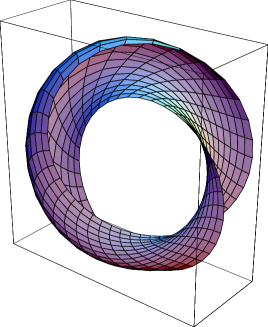
Figure 3. Stereographic projection from ${\mathbb{S}^{3}}-\{\text{north pole}\}$ to ${\mathbb{R}}^{3}$ of one half of the surface $\mathcal{C}_{0,\lambda}$. It consists of the union of all the geodesics of curvature $\lambda$ and length $\pi/(2\sqrt{1+\lambda^{2}})$ connecting two singular circles.

In Figure 3 we see that the surface $\Sigma_{\lambda}(\Gamma)$ is embedded. To prove this note that the function $(x_{1}y_{1}+x_{2}y_{2})(\varepsilon,s)$ only depends on $s$, and its first derivative with respect to $s$ equals $(1+\lambda^{2})^{-1/2}\,\sin(2\lambda s)\,\sin(2\sqrt{1+\lambda^{2}}\,s)$, which does not change sign on $(0,\pi/(2\sqrt{1+\lambda^{2}}))$. Thus if $F(\varepsilon_{1},s_{1})=F(\varepsilon_{2},s_{2})$ for some $\varepsilon_{i}\in[0,2\pi)$ and $s_{i}\in[0,\pi/(2\sqrt{1+\lambda^{2}})]$ then $s_{1}=s_{2}$, which clearly implies $\varepsilon_{1}=\varepsilon_{2}$. Similarly we obtain that $\widetilde{\Sigma}_{\lambda}(\Gamma)$ is embedded. On the other hand, observe that $2(x_{1}y_{2}-x_{2}y_{1})(\varepsilon,s)=\sin(2\sqrt{1+\lambda^{2}}\,s)/\sqrt{1+\lambda^{2}}$ on $\Sigma_{\lambda}(\Gamma)$, whereas the same function evaluated on $\widetilde{\Sigma}_{\lambda}$ equals $-\sin(2\sqrt{1+\lambda^{2}}\,s)/\sqrt{1+\lambda^{2}}$. It follows that $\mathcal{C}_{0,\lambda}$ is an embedded surface outside the singular curves. Finally, a long but easy computation shows that there is a system of coordinates $(u_{1},u_{2},u_{3},u_{4})$ such that $\mathcal{C}_{0,\lambda}$ can be expressed as union of certain graphs $u_{1}=f_{i}(u_{2},u_{3})$ and $u_{4}=g_{i}(u_{2},u_{3})$, $i=1,2$, defined over an annulus of the $u_{2}u_{3}$-plane. The functions $f_{i}$ and $g_{i}$ are $C^{2}$ near the singular curves. This proves that $\mathcal{C}_{0,\lambda}$ is a volume-preserving area-stationary embedded torus with two singular curves.

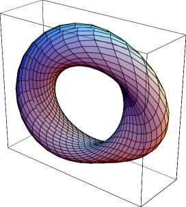
Figure 4. Stereographic projection from ${\mathbb{S}^{3}}-\{\text{north pole}\}$ to ${\mathbb{R}}^{3}$ of an embedded torus $\mathcal{C}_{0,\lambda}$.

Example 5.8 (The surfaces $\mathcal{C}_{\mu,\lambda}$).

Let $\Gamma$ be the geodesic of curvature $\mu$ in $({\mathbb{S}^{3}},g_{h})$ with initial conditions $p=(1,0,0,0)$ and $v=E_{1}(p)$. We know that the function $h=\big{<}\ddot{\Gamma},J(\dot{\Gamma})\big{>}$ equals $-2\mu$ along $\Gamma$ by Lemma 3.2. For any $\lambda\in{\mathbb{R}}$ we consider the union $\Sigma_{\lambda}(\Gamma)\cup\widetilde{\Sigma}_{\lambda}(\Gamma)$, which is a $C^{\infty}$ surface with constant mean curvature $\lambda$ outside the singular curves $\Gamma$, $\Gamma_{1}$ and $\Gamma_{2}$. By using Lemma 3.2 (ii) we can prove that any $\Gamma_{i}$ is a geodesic of curvature $\mu$. The cut functions $s_{\varepsilon}$ and $\widetilde{s}_{\varepsilon}$ are determined by equalities (5.4) and (5.5). Define $\varepsilon_{\mu}$ as the unique $\varepsilon\in(0,\pi/\sqrt{1+\mu^{2}})$ such that $\cot(\sqrt{1+\mu^{2}}\,\varepsilon_{\mu})=-\lambda/\sqrt{1+\mu^{2}}$. Let $\widetilde{\varepsilon}_{\mu}=\pi/\sqrt{1+\mu^{2}}-\varepsilon_{\mu}$. Easy computations from (5.3) show that

$$\Gamma_{1}(s_{\mu})=\exp(i\theta_{1})\cdot p,\quad\dot{\Gamma}_{1}(s_{\mu})=\exp(i\theta_{1})\cdot v,$$

$$\Gamma_{2}(\tilde{s}_{\mu})=\exp(i\theta_{2})\cdot p,\quad\dot{\Gamma}_{2}(\tilde{s}_{\mu})=\exp(i\theta_{2})\cdot v,$$

where $\theta_{1}=3\pi/2-\lambda s_{\varepsilon}-\mu\varepsilon_{\mu}$ and $\theta_{2}=\pi/2-\lambda\widetilde{s}_{\varepsilon}-\mu\widetilde{\varepsilon}_{\mu}$. By the uniqueness of the geodesics we deduce that $\Gamma_{1}(\varepsilon+\varepsilon_{\mu})=\exp(i\theta_{1})\cdot\Gamma(\varepsilon)$ and $\Gamma_{2}(\varepsilon+\widetilde{\varepsilon}_{\mu})=\exp(i\theta_{2})\cdot\Gamma(\varepsilon)$. In general $\Gamma_{1}\neq\Gamma_{2}$ so that we can extend the surface by geodesics orthogonal to $\Gamma_{i}$ of the same curvature. As we pointed out in Remark 5.6 and according with the initial velocity of $\Gamma_{i}$, in order to preserve the constant mean curvature $\lambda$ we must consider the surfaces $\widetilde{\Sigma}_{-\lambda}(\Gamma_{1})$ and $\Sigma_{-\lambda}(\Gamma_{2})$. Two new singular curves $\Gamma_{12}$ and $\Gamma_{22}$ are obtained. It is straightforward to check that, after a translation of the parameter $\varepsilon$, we have $\Gamma_{12}=\exp(i\theta_{12})\cdot\Gamma$ and $\Gamma_{22}=\exp(i\theta_{22})\cdot\Gamma$, where $\theta_{12}=\theta_{1}+\pi/2+\lambda\tilde{s}_{\varepsilon}-\mu\varepsilon_{\mu}$ and $\theta_{22}=\theta_{2}+3\pi/2+\lambda s_{\varepsilon}-\mu\tilde{\varepsilon}_{\mu}$. Let $\tilde{\theta}_{1}=\theta_{12}-\theta_{1}$ and $\tilde{\theta}_{2}=\theta_{22}-\theta_{2}$. We repeat this process by induction so that at any step $k+1$ we leave from the singular curves $\Gamma_{1k}$ and $\Gamma_{2k}$ by the corresponding orthogonal geodesics of curvature $(-1)^{k}\lambda$. We denote by $\mathcal{C}_{\mu,\lambda}$ the union of all these surfaces. After a translation of $\varepsilon$, any singular curve $\Gamma_{jk}$ is of the form $\exp(i\theta_{jk})\cdot\Gamma$, where the angles are given by $\theta_{j\,2m}=m(\theta_{j}+\tilde{\theta}_{j})$ and $\theta_{j\,2m+1}=(m+1)\theta_{j}+m\tilde{\theta}_{j}$. This implies that all the singular curves are geodesics of curvature $\mu$ and their projections to ${\mathbb{S}}^{2}$ via the Hopf fibration give the same geodesic circle. It follows by uniqueness of the horizontal lifts that two singular curves meeting at one point must coincide as subsets of ${\mathbb{S}^{3}}$. In fact it is possible that two singular curves coincide. For example, the surface $\mathcal{C}_{\mu,0}$ is a compact surface with two or four singular curves (depending on if $\mu/\sqrt{1+\mu^{2}}$ is rational or not). On the other hand it can be shown that if $\mu/\sqrt{1+\mu^{2}}$ and $\lambda/\sqrt{1+\lambda^{2}}$ are rational numbers and $(\lambda s_{\varepsilon}+\mu\varepsilon_{\mu})/\pi$ is irrational (take $\lambda=\mu=1/\sqrt{3}$) then $\mathcal{C}_{\mu,\lambda}$ is a noncompact surface with infinitely many singular curves.

The surface $\mathcal{C}_{\mu,\lambda}$ is $C^{\infty}$ off of the singular set and has constant mean curvature $\lambda$. A necessary condition to get a surface which is also $C^{2}$ near the singular curves is that $\Gamma$ locally separates $\mathcal{C}_{\mu,\lambda}$ into two disjoint domains, see Theorem 4.3 (ii). By Proposition 3.3 this is equivalent to that $\mu/\sqrt{1+\mu^{2}}$ is a rational number. In such a case $\mathcal{C}_{\mu,\lambda}$ is a volume-preserving area-stationary surface by construction. In general the surfaces $\mathcal{C}_{\mu,\lambda}$ are not embedded.

Now we can classify complete area-stationary surfaces under a volume constraint with a non-empty set of singular curves.

Theorem 5.9.

Let $\Sigma$ be a complete, oriented, connected, $C^{2}$ immersed surface. Suppose that $\Sigma$ is volume-preserving area-stationary in $({\mathbb{S}^{3}},g_{h})$ and $\Gamma$ is a connected singular curve of $\Sigma$. Then $\Gamma$ is a closed geodesic, and $\Sigma$ is congruent with a surface $\mathcal{C}_{\mu,\lambda}$.

Proof.

By Theorem 4.5 we have that $\Gamma$ is a $C^{2}$ horizontal curve. We can assume that $\Gamma$ is parameterized by arc-length. We take the unit normal $N$ to $\Sigma$ such that $N=V$ along $\Gamma$. Let $H$ be the mean curvature of $\Sigma$ with respect to $N$. Let $p\in\Gamma$. By Theorem 4.3 (ii) and Remark 4.4 there is a small neighborhood $B$ of $p$ in $\Sigma$ such that $B\cap\Gamma$ is a connected curve separating $B$ into two disjoint connected open sets foliated by geodesics $\gamma_{\varepsilon}$ of curvature $\lambda=H$ leaving from $\Gamma$. These geodesics are characteristic curves of $\Sigma$. Moreover, by Theorem 4.5 they must leave from $\Gamma$ orthogonally. As $\Sigma$ is complete and connected we deduce that any $\gamma_{\varepsilon}$ can be extended until it meets a singular point. Thus there exists a small piece $\Gamma^{\prime}\subset\Gamma$ containing $p$ and such that $\Sigma_{\lambda}(\Gamma^{\prime})\subset\Sigma$. In particular we find another singular curve $\Gamma_{1}^{\prime}$ of $\Sigma$ which is also $C^{2}$ smooth by Theorem 4.5. As $\Sigma$ is volume-preserving area-stationary, any $\gamma_{\varepsilon}$ meet $\Gamma_{1}^{\prime}$ orthogonally and so $\Gamma^{\prime}$ is a geodesic by Proposition 5.5 (v). Since $p\in\Gamma$ is arbitrary we have proved that $\Gamma$ is a geodesic in $({\mathbb{S}^{3}},g_{h})$. That $\Gamma$ is closed follows from Proposition 3.3; otherwise, the intersection of $\Gamma$ with any open neighborhood of $p$ in $\Sigma$ would have infinitely many connected components, a contradiction with Theorem 4.3 (ii). After applying a right translation $R_{q}$ and a rotation $r_{\theta}$ we can suppose that $\Gamma$ leaves from $p=(1,0,0,0)$ with velocity $v=E_{1}(p)$. By using again the local description of $\Sigma$ around $\Gamma$ in Theorem 4.3 (ii) together with the completeness and the connectedness of $\Sigma$, we conclude that $\Sigma$ is congruent with $\mathcal{C}_{\mu,\lambda}$. ∎

5.3. Complete surfaces with empty singular set

Here we prove some classification results for complete constant mean curvature surfaces with empty singular set. Such a surface must be area-stationary with or without a volume constraint by Theorem 4.5. Moreover, if the surface is compact then it must be homeomorphic to a torus by Theorem 4.7.

The following result uses the behaviour of geodesics in $({\mathbb{S}^{3}},g_{h})$ described in Proposition 3.3 to establish a strong restriction on a compact embedded surface with constant mean curvature.

Theorem 5.10.

Let $\Sigma$ be a $C^{2}$ compact, connected, embedded surface in $({\mathbb{S}^{3}},g_{h})$ without singular points. If $\Sigma$ has constant mean curvature $H$ such that $H/\sqrt{1+H^{2}}$ is an irrational number, then $\Sigma$ is congruent with a Clifford torus.

Proof.

As $\Sigma$ is compact with empty singular set we deduce by Theorem 4.2 that there is a complete geodesic $\gamma$ of curvature $H$ contained in $\Sigma$. After a right translation $R_{q}$ we have, by Proposition 3.3, that $R_{q}(\gamma)$ is a dense subset of a Clifford torus $\mathcal{T}_{\rho}$. By using that $\Sigma$ is compact, connected and embedded we conclude that $R_{q}(\Sigma)=\mathcal{T}_{\rho}$, proving the claim. ∎

In Remark 6.6 we will give examples showing that all the hypotheses Theorem 5.10 are necessary. We finish this section with a characterization of the Clifford tori $\mathcal{T}_{\rho}$ as the unique vertical surfaces with constant mean curvature. We say that a $C^{1}$ surface $\Sigma\subset{\mathbb{S}^{3}}$ is vertical if the vector field $V$ is tangent to $\Sigma$.

Proposition 5.11.

Let $\Sigma$ be a $C^{2}$ complete, connected, oriented, constant mean curvature surface in $({\mathbb{S}^{3}},g_{h})$. If $\Sigma$ is vertical then $\Sigma$ is congruent with a Clifford torus.

Proof.

It is clear that $\Sigma$ has no singular points. Thus we can find by Theorem 4.2 a complete geodesic $\gamma$ contained in $\Sigma$. By Proposition 3.3 there is a point $q\in{\mathbb{S}^{3}}$ such that $R_{q}(\gamma)$ is contained inside a Clifford torus $\mathcal{T}_{\rho}$. By assumption, the vertical great circle passing through any point of $\gamma$ is entirely contained in $R_{q}(\Sigma)$. Clearly the union of all these circles is $\mathcal{T}_{\rho}$. Finally as $\Sigma$ is complete and connected we conclude that $R_{q}(\Sigma)=\mathcal{T}_{\rho}$. ∎

6. Rotationally invariant constant mean curvature surfaces

In this section we classify $C^{2}$ constant mean curvature surfaces of revolution in $({\mathbb{S}^{3}},g_{h})$. We will follow arguments similar to those in [RR, §5].

Let $R$ be the great circle given by the intersection of ${\mathbb{S}^{3}}$ with the $x_{1}y_{1}$-plane. The rotation $r_{\theta}$ of the $x_{2}y_{2}$-plane defined in (2.5) is an isometry of $({\mathbb{S}^{3}},g)$ leaving invariant the horizontal distribution and fixing $R$. Let $\Sigma$ be a $C^{2}$ surface in ${\mathbb{S}^{3}}$ which is invariant under any rotation $r_{\theta}$. We denote by $\gamma$ the generating curve of $\Sigma$ inside the hemisphere ${\mathbb{S}}^{2}_{+}:=\{x_{2}\geqslant 0,y_{2}=0\}$. If we parameterize $\gamma=(x_{1},y_{1},x_{2})$ by arc-length $s\in I$, then $\Sigma-R$ is given in cylindrical coordinates by $\phi(s,\theta)=r_{\theta}(\gamma(s))=(x_{1}(s),y_{1}(s),x_{2}(s)\cos\theta,x_{2}(s)\sin\theta)$. Denote by $\{e_{1},e_{2}\}$ the usual orthonormal frame in the Euclidean plane. The tangent plane to $\Sigma-R$ is generated by the vector fields $\partial_{1}:=e_{1}(\phi)$ and $\partial_{2}:=e_{2}(\phi)$. Note that $|\partial_{1}|=1$, $|\partial_{2}|=x_{2}$ and $\big{<}\partial_{1},\partial_{2}\big{>}=0$. A unit normal vector along $\phi$ is given by

(6.1) $$N=(x_{2}\dot{y}_{1}-\dot{x}_{2}y_{1},x_{1}\dot{x}_{2}-\dot{x}_{1}x_{2},(\dot{x}_{1}y_{1}-x_{1}\dot{y}_{1})\cos\theta,(\dot{x}_{1}y_{1}-x_{1}\dot{y}_{1})\sin\theta).$$

It follows that $|N_{h}|^{2}=\big{<}N,E_{1}\big{>}^{2}+\big{<}N,E_{2}\big{>}^{2}=(\dot{x}_{1}y_{1}-x_{1}\dot{y}_{1})^{2}+x_{2}^{2}$. In particular, the singular points of $\Sigma$ are contained inside $R$.

Now we compute the mean curvature $H$ of $\Sigma-R$ with respect to the normal $N$ defined in (6.1). By equality (4.4) we know that $2H=|N_{h}|^{-1}\text{II}(Z,Z)$ and so, it is enough to compute the second fundamental form II of $\phi$ with respect to $N$. It is clear that the coefficients of II in the basis $\{\partial_{1},\partial_{2}\}$ are given by $\text{II}_{ij}=\text{II}(\partial_{i},\partial_{j})=-\big{<}D_{\partial_{i}}N,\partial_{j}\big{>}=\big{<}N,D_{e_{i}}\partial_{j}\big{>}$. On the other hand, if $(a_{1j},a_{2j},a_{3j})$ are the coordinates of $\partial_{j}$ in the orthonormal basis $\{E_{1},E_{2},V\}$, then a straightforward calculation by using (2.1) shows that the coordinates of $D_{e_{i}}\partial_{j}$ with respect to $\{E_{1},E_{2},V\}$ are

$$\left(\frac{\partial a_{1j}}{\partial e_{i}}+a_{3i}\,a_{2j}-a_{2i}\,a_{3j},\frac{\partial a_{2j}}{\partial e_{i}}-a_{3i}\,a_{1j}+a_{1i}\,a_{3j},\frac{\partial a_{3j}}{\partial e_{i}}+a_{2i}\,a_{1j}-a_{1i}\,a_{2j}\right).$$

This allows us to compute $\text{II}_{ij}$ and we obtain the following

$$\text{II}_{11} =x_{2}\,(\ddot{x}_{1}\dot{y}_{1}-\dot{x}_{1}\ddot{y}_{1})-\dot{x}_{2}\,(\ddot{x}_{1}y_{1}-x_{1}\ddot{y}_{1})+\ddot{x}_{2}\,(\dot{x}_{1}y_{1}-x_{1}\dot{y}_{1}),$$

$$\text{II}_{12} =\text{II}_{21}=0,$$

$$\text{II}_{22} =x_{2}\,(x_{1}\dot{y}_{1}-\dot{x}_{1}y_{1}).$$

On the other hand, the coordinates of the characteristic vector field $Z$ with respect to $\{\partial_{1},\partial_{2}\}$ are $\big{<}Z,\partial_{1}\big{>}$ and $x^{-2}_{2}\big{<}Z,\partial_{2}\big{>}$. Thus we can use equation (4.4) to deduce that the mean curvature of $\Sigma-R$ with respect to $N$ is

$$2H=\frac{(x_{1}\dot{y}_{1}-\dot{x}_{1}y_{1})^{3}+x_{2}^{3}\,\{x_{2}\,(\ddot{x}_{1}\dot{y}_{1}-\dot{x}_{1}\ddot{y}_{1})-\dot{x}_{2}\,(\ddot{x}_{1}y_{1}-x_{1}\ddot{y}_{1})+\ddot{x}_{2}\,(\dot{x}_{1}y_{1}-x_{1}\dot{y}_{1})\}}{x_{2}\,(\dot{x}_{1}+\dot{y}_{1})^{3/2}}.$$

Now we take spherical coordinates $(\omega,\tau)$ in ${\mathbb{S}}^{2}\equiv\{y_{2}=0\}$. In precise terms, we choose $\omega\in(-\pi/2,\pi/2)$ and $\tau\in{\mathbb{R}}$ so that the Euclidean coordinates of a point in ${\mathbb{S}}^{2}$ different from the poles can be expressed as $x_{1}=\cos\omega\,\cos\tau$, $y_{1}=\cos\omega\,\sin\tau$ and $x_{2}=\sin\omega$. The vector fields $\partial_{\omega}$ and $\partial_{\tau}/(\cos\omega)$ provide an orthonormal basis of the tangent plane to ${\mathbb{S}}^{2}$ off of the poles. The integral curves of $\partial_{\omega}$ and $\partial_{\tau}$ are the meridians and the circles of revolution about the $x_{2}$-axis, respectively.

Let $(\omega(s),\tau(s))$ with $\omega(s)\in[0,\pi/2)$ be the spherical coordinates of the generating curve $\gamma(s)$. Denote by $\sigma(s)$ the oriented angle between $\partial_{\omega}$ and $\dot{\gamma}(s)$. Then we have $\dot{\omega}=\cos\sigma$ and $\dot{\tau}=(\sin\sigma)/(\cos\omega)$. Now we replace Euclidean coordinates with spherical coordinates in the expression given above for the mean curvature $H$ of $\Sigma-R$ and we get

Lemma 6.1.

The generating curve $\gamma=(\omega,\tau)$ in ${\mathbb{S}}^{2}_{+}$ of a $C^{2}$ surface which is invariant under any rotation $r_{\theta}$ and has mean curvature $H$ in $({\mathbb{S}^{3}},g_{h})$ satisfies the following system of ordinary differential equations

$$(*)_{H}\quad\left\{\begin{aligned} \dot{\omega}&=\cos\sigma,\\ \dot{\tau}\,&=\frac{\sin\sigma}{\cos\omega},\\ \dot{\sigma}&=\tan\omega\,\sin\sigma-\cot^{3}\omega\,\sin^{3}\sigma+2H\,\,\frac{(\sin^{2}\omega\,\cos^{2}\sigma+\sin^{2}\sigma)^{3/2}}{\sin^{2}\omega},\end{aligned}\right.$$

whenever $\omega\in(0,\pi/2)$. Moreover, if $H$ is constant then the function

(6.2) $$\frac{\sin\omega\,\cos\omega\,\sin\sigma}{\sqrt{\sin^{2}\omega\,\cos^{2}\sigma+\sin^{2}\sigma}}-H\sin^{2}\omega$$

is constant along any solution of $(*)_{H}$.

Note that the system $(*)_{H}$ has singularities for $\omega=0,\pi/2$. We will show that the possible contact between a solution $(\omega,\tau,\sigma)$ and $R$ is perpendicular. This means that the generated surface $\Sigma$ is of class $C^{1}$ near $R$.

The existence of a first integral for $(*)_{H}$ follows from Noether’s theorem [GiH, §4 in Chap. 3] by taking into account that the translations along the $\tau$-axis preserve the solutions of $(*)_{H}$. The constant value $E$ of the function (6.2) will be called the energy of the solution $(\omega,\tau,\sigma)$. Notice that

$$\sin\omega\,\cos\omega\,\sin\sigma=(E+H\sin^{2}\omega)\,\sqrt{\sin^{2}\omega\,\cos^{2}\sigma+\sin^{2}\sigma}.$$

The equation above clearly implies

(6.3) $$(\sin^{2}\omega\,\cos^{2}\omega-(E+H\sin^{2}\omega)^{2})\,\sin^{2}\sigma=(E+H\sin^{2}\omega)^{2}\sin^{2}\omega\,\cos^{2}\sigma,$$

from which we deduce the inequality

(6.4) $$\sin\omega\,\cos\omega\geqslant|E+H\sin^{2}\omega|,$$

which is an equality if and only if $\cos\sigma=0$.

Moreover, by using (6.3) we get

(6.5) $$\sin\sigma=\frac{(E+H\sin^{2}\omega)\,\sin\omega}{\cos\omega\,\sqrt{\sin^{2}\omega-(E+H\sin^{2}\omega)^{2}}}.$$

By substituting (6.5) in the third equation of $(*)_{H}$ we deduce

(6.6) $$\dot{\sigma}=\frac{p(\sin^{2}\omega)}{\cos^{2}\omega\,(\sin^{2}\omega-(E+H\sin^{2}\omega)^{2})^{3/2}},$$

where $p$ is the polynomial given by $p(x)=-(E+Hx)^{3}-Hx^{3}+(E+2H)x^{2}$.

From the uniqueness of the solutions of $(*)_{H}$ for given initial conditions we easily obtain

Lemma 6.2.

Let $(\omega(s),\tau(s),\sigma(s))$ be a solution of $(*)_{H}$ with energy $E$. Then, we have

• The solution can be translated along the $\tau$-axis. More precisely, $(\omega(s),\tau(s)+\tau_{0},\sigma(s))$ is a solution of $(*)_{H}$ with energy $E$ for any $\tau_{0}\in{\mathbb{R}}$.

• The solution is symmetric with respect to any meridian $\{\tau=\tau(s_{0})\}$ such that $\dot{\omega}(s_{0})=0$. As a consequence, we can continue a solution by reflecting across the critical points of $\omega(s)$.

• The curve $(\omega(s_{0}-s),\tau(s_{0}-s),\pi+\sigma(s_{0}-s))$ is a solution of $(*)_{-H}$ with energy $-E$.

Lemma 6.3.

Let $(\omega(s),\tau(s),\sigma(s))$ be a solution of $(*)_{H}$. If $\sin\sigma(s_{0})\neq 0$, then the coordinate $\omega$ is a function over a small $\tau$-interval around $\tau(s_{0})$. Moreover

(6.7) $$\frac{d\omega}{d\tau}=\cos\omega\,\cot\sigma,\qquad\frac{d^{2}\omega}{d\tau^{2}}=-\frac{\sin\omega\,\cos\omega\,\sin\sigma\,\cos^{2}\sigma+\dot{\sigma}\,\cos^{2}\omega}{\sin^{3}\sigma},$$

where $\dot{\sigma}$ is the derivative of $\sigma$ with respect to $s$.

Now we describe the complete solutions of $(*)_{H}$. They are of the same types as the ones obtained by W. Y. Hsiang [Hs] when he studied constant mean curvature surfaces of revolution in $({\mathbb{S}^{3}},g)$.

Theorem 6.4.

Let $\gamma$ be the generating curve of a $C^{2}$ complete, connected, rotationally invariant surface $\Sigma$ with constant mean curvature $H$ and energy $E$. Then the surface $\Sigma$ must be of one of the following types

• If $H=0$ and $E=0$ then $\gamma$ is a half-meridian and $\Sigma$ is a totally geodesic $2$-sphere in $({\mathbb{S}^{3}},g)$.

• If $H=0$ and $E\neq 0$ then $\Sigma$ coincides either with the minimal Clifford torus $\mathcal{T}_{\sqrt{2}/2}$ or with a compact embedded surface of unduloidal type.

• If $H\neq 0$ and $E=0$ then $\Sigma$ is a compact surface congruent with a sphere $\mathcal{S}_{H}$.

• If $EH\neq 0$ and $H\neq-E$ then $\Sigma$ coincides either with a non-minimal Clifford torus $\mathcal{T}_{\rho}$, or with an unduloidal type surface, or with a nodoidal type surface which has selfintersections. Moreover, unduloids and nodoids are compact surfaces if and only if $H/\sqrt{1+H^{2}}$ is a rational number.

• If $H=-E$ then $\gamma$ consists of a union of circles meeting at the north pole. The generated $\Sigma$ is a compact surface if and only if $H/\sqrt{1+H^{2}}$ is a rational number.

Figure 5. Generating curves in spherical coordinates of rotationally invariant surfaces with constant mean curvature in $({\mathbb{S}^{3}},g_{h})$. The horizontal segments represent the $\tau$-axis and the line $\omega=\pi/2$, which is identified with the north pole. The vertical segment represents the $\omega$-axis. The generated surfaces are, respectively, a totally geodesic $2$-sphere, a Clifford torus, a spherical surface $\mathcal{S}_{\lambda}$, an unduloidal type surface, a nodoidal type surface, and a surface consisting of “petals” meeting at the north pole.

Proof.

By removing the points where the generating curve meets the north pole and $R$, we can suppose that $\gamma=(\omega,\tau,\sigma)$ is a complete solution of $(*)_{H}$ with energy $E$. By Lemma 6.2 (i) we can assume that $\gamma$ is defined over an open interval $I$ containing the origin, and that the initial conditions are $(\omega_{0},0,\sigma_{0})$. We can also suppose that $H\geqslant 0$ by Lemma 6.2 (iii).

To prove the theorem we distinguish several cases depending on the value of $E$.

$\bullet$ $E=0$. Suppose first that $H=0$. Then $\sin\sigma\equiv 0$ along $\gamma$ from (6.5) and so, the solution is given by $\tau\equiv 0$, $\omega(s)=s+\omega_{0}$ and $\sigma\equiv 0$. We conclude that $\gamma$ is a half-meridian. The generated surface is a totally geodesic $2$-sphere in $({\mathbb{S}^{3}},g)$ with two isolated singular points.

Now suppose $H>0$. In this case we get $\sin\sigma>0$ by (6.5) and so we can see the $\omega$-coordinate as a function of $\tau$. Moreover, $\tan\omega\leqslant 1/H$ by (6.4), so that the solution could approach the $\tau$-axis. We can take the initial conditions of $\gamma$ as $(\arctan(H^{-1}),0,\pi/2)$. By the symmetry of the solutions we only have to study the function $\omega(\tau)$ for $\tau>0$. By using (6.6) we obtain $\dot{\sigma}>0$, which together with the fact that $\sin\sigma>0$, implies that $\sigma\in(\pi/2,\pi)$. Therefore $\cos\sigma<0$ and the function $\omega(\tau)$ is strictly decreasing. In addition $\sin\sigma\rightarrow 0$ as $\omega\rightarrow 0$ by (6.5) and so, $\gamma$ meets the $\tau$-axis orthogonally.

On the other hand as $\cos\sigma<0$ we can see the $\tau$-coordinate as a function of $\omega$. This function satisfies that

$$\frac{d\tau}{d\omega}=\frac{-H\,\sin^{2}\omega}{\cos\omega\,\sqrt{\cos^{2}\omega-H^{2}\sin^{2}\omega}},\qquad\omega\in(0,\arctan(H^{-1})).$$

We can integrate the equality above to conclude that

$$\tau(\omega)=\frac{H}{\sqrt{1+H^{2}}}\arcsin(\sqrt{1+H^{2}}\sin\omega)-\arcsin(H\tan\omega)+\frac{\pi}{2}\,\left(1-\frac{H}{\sqrt{1+H^{2}}}\right).$$

Finally it is easy to see that, after a translation along the $\tau$-axis, the expression of the generated $\Sigma$ in Euclidean coordinates coincides with the one given in (5.1) for the sphere $S_{H}$.

$\bullet$ $E\neq 0$. From (6.4) we get that $(1+H^{2})\sin^{4}\omega-(1-2EH)\sin^{2}\omega+E^{2}\leqslant 0$, which implies that $(1-2EH)^{2}-4E^{2}(1+H^{2})\geqslant 0$. In this case, $\omega_{1}\leqslant\omega\leqslant\omega_{2}$, where $\sin\omega_{1}$ and $\sin\omega_{2}$ coincide with the positive zeroes of the polynomial $(1+H^{2})x^{4}-(1-2EH)x^{2}+E^{2}$. Therefore the solution does not approach the $\tau$-axis. We distinguish several cases:

(i) $E>0$. If $(1-2EH)^{2}-4E^{2}(1+H^{2})=0$ ($\omega_{1}=\omega_{2}$) then $E=(\sqrt{1+H^{2}}-H)/2$ and the solution is given by

$$\omega\equiv\arcsin\Big{(}\sqrt{\frac{1}{2}-\frac{H}{2\sqrt{1+H^{2}}}}\Big{)}.$$

The generated $\Sigma$ is the Clifford torus $\mathcal{T}_{\rho}$ with $\rho^{2}=(1/2)(1+H/\sqrt{1+H^{2}})$. Otherwise, by equation $\eqref{eq:seno}$ we get that $\sin\sigma>0$ and then the $\omega$-coordinate is a function of $\tau$. After a translation along the $\tau$-axis we can suppose that the initial conditions of $\gamma$ are $(\omega_{1},0,\pi/2)$. Moreover, by symmetry of the solutions, it is enough to study $\omega(\tau)$ for $\tau>0$.

Call $s_{2}$ to the first $s>0$ such that $\sigma(s)=\pi/2$. Taking into account (6.6), it is easy to see that there exists a unique $s_{1}\in(0,s_{2})$ such that $\dot{\sigma}(s_{1})=0$. By the definition of $s_{1}$ and $s_{2}$ we get $\dot{\sigma}<0$ on $(0,s_{1})$ and $\dot{\sigma}>0$ on $(s_{1},s_{2})$, so that $\sigma$ reaches a minimal value in $\sigma(s_{1})$. As a consequence, $\sigma\in(0,\pi/2)$ and $\cos\sigma>0$ on $(0,s_{2})$. Thus, if we define $\tau_{2}=\tau(s_{2})$ then the function $\omega(\tau)$ is strictly increasing on $(0,\tau_{2})$ and so, $\omega(\tau_{2})=\omega_{2}$. On the other hand by substituting (6.5) and (6.6) into (6.7) we get

(6.8) $$\frac{d^{2}\omega}{d\tau^{2}}=\frac{\cos\omega}{\sin^{3}\omega\,(E+H\sin^{2}\omega)^{3}}\,((E+H\sin^{2}\omega)^{3}-2(E+H)\sin^{4}\omega\cos^{2}\omega).$$

It follows that there exists a unique value $\tau_{1}\in(0,\tau_{2})$ such that $(d^{2}\omega/d\tau^{2})(\tau_{1})=0$. We can conclude that the graph $\omega(\tau)$ is strictly increasing and strictly convex on $(0,\tau_{1})$ whereas it is strictly increasing and strictly concave on $(\tau_{1},\tau_{2})$. By successive reflections across the vertical lines on which $\omega(\tau)$ reaches its critical points, we get the full solution which is periodic and similar to a Euclidean unduloid.

As $\cos\sigma>0$ on $(0,s_{2})$, we can see the $\tau$-coordinate as a function of $\omega\in(\omega_{1},\omega_{2})$. Then, the period of $\gamma$ is given by

$$T=2\int_{\omega_{1}}^{\omega_{2}}\dot{\tau}(\omega)\,d\omega=2\int_{\omega_{1}}^{\omega_{2}}\frac{(E+H\sin^{2}\omega)\,\sin\omega}{\cos\omega\,\sqrt{\cos^{2}\omega\,\sin^{2}\omega-(E+H\sin^{2}\omega)^{2}}}\,\,d\omega.$$

A straightforward computation shows that $T=(1-H/\sqrt{1+H^{2}})\pi$. Then the generated $\Sigma$ is an unduloidal type surfaces which is compact if and only if $H/\sqrt{1+H^{2}}$ is a rational number. Moreover, $\Sigma$ is embedded if and only if $T=2\pi/k$ for some integer $k$. In the particular case of $H=0$, we have proved that the generated $\Sigma$ is either the minimal Clifford torus or a compact embedded unduloidal type surface.

(ii) $E<0$. Assuming that $H<-E$ we get that $\sin\sigma<0$ along $\gamma$ by (6.5). By using the same arguments as in the previous case we deduce that $\Sigma$ coincides either with the Clifford torus $\mathcal{T}_{\rho}$ with $\rho^{2}=(1/2)(1-H/\sqrt{1+H^{2}})$, or with an unduloidal type surface with period $T=(1+H/\sqrt{1+H^{2}})\,\pi$. Hence these unduloidal surfaces are never embedded. Moreover they are compact if and only if $H/\sqrt{1+H^{2}}$ is a rational number.

Thus we can suppose $H>-E$. In this case we have $\sin\sigma<0$ if $\sin\omega\in[\sin\omega_{1},\sqrt{-E/H})$ while $\sin\sigma>0$ if $\sin\omega\in(\sqrt{-E/H},\sin\omega_{2}]$. Moreover, from (6.6) it is easy to check that $\dot{\sigma}>0$ along the solution. After a translation along the $\tau$-axis, we can suppose that the initial conditions of $\gamma$ are $(\omega_{2},0,\pi/2)$. By the symmetry property we only have to study the solution for $s>0$.

Call $s_{1}$ and $s_{2}$ to the first positive numbers such that $s_{1}<s_{2}$, $\sigma(s_{1})=\pi$ and $\sigma(s_{2})=3\pi/2$. Then $\omega(s_{1})=\sqrt{-E/H}$ and $\omega(s_{2})=\omega_{1}$. Call $\tau_{i}=\tau(s_{i})$, $i=1,2$. We have that $\sigma\in(\pi/2,\pi)$ on $(0,s_{1})$ and $\sigma\in(\pi,3\pi/2)$ on $(s_{1},s_{2})$. As a consequence, the restriction of $\gamma$ to $[0,s_{2}]$ consists of two graphs of the function $\omega(\tau)$ meeting at $\tau=\tau_{1}$. Taking into account (6.8) we can conclude that $\omega(\tau)$ is strictly decreasing and strictly concave on $(0,\tau_{1})$ whereas it is strictly increasing and strictly convex on $(\tau_{2},\tau_{1})$. As $\{\tau=0\}$ and $\{\tau=\tau_{2}\}$ are lines of symmetry for $\gamma$, we can reflect successively to obtain the complete solution, which is periodic. The generating curve is embedded if and only if $\tau_{2}=0$. Let us see that this is not possible.

As $\cos\sigma<0$ on $(0,s_{2})$, we can see the $\tau$-coordinate as a function of $\omega$. Then,

$$\tau_{2}=-\int_{\omega_{1}}^{\omega_{2}}\dot{\tau}(\omega)\,d\omega=\int_{\omega_{1}}^{\omega_{2}}\frac{(E+H\sin^{2}\omega)\,\sin\omega}{\cos\omega\,\sqrt{\cos^{2}\omega\sin^{2}\omega-(E+H\sin^{2}\omega)^{2}}}\,\,d\omega.$$

A straightforward computation shows that

$$\tau_{2}=\frac{\pi}{2}\,\Big{(}1-\frac{H}{\sqrt{1+H^{2}}}\Big{)}>0.$$

It follows that the period of $\gamma$ is given by $(1-H/\sqrt{1+H^{2}})\pi$, and $\Sigma$ is a nodoidal type surface which is compact if and only if $H/\sqrt{1+H^{2}}$ is a rational number.

To finish the prove we only have to study the case $H=-E$. Now $\sin\omega_{1}=H/\sqrt{1+H^{2}}$ and $\sin\omega_{2}=1$. Then the solution could approach the north pole. Note that $\sin\sigma<0$ far away of the north pole by (6.5). Thus along any connected component of $\gamma-\{\text{pole}\}$ we can see the $\omega$-coordinate as a function of $\tau$. Using (6.5) and the expressions of $\dot{\sigma}$ and $d^{2}\omega/d\tau^{2}$ given by $(*)_{H}$ and (6.8) respectively, it is easy to see that $\dot{\sigma}>0$ if $\omega\neq\pi/2$ and that $d^{2}\omega/d\tau^{2}>0$. In addition, $\sin\sigma\rightarrow 0$ as $\omega\rightarrow\pi/2$. We can suppose that the initial conditions of $\gamma$ are $(\omega_{1},0,3\pi/2)$. By the symmetry of the solution, we only have to study $\gamma(s)$ for $s>0$.

Call $s_{0}$ to the first $s>0$ such that $\sin\sigma(s)=0$. As $\sigma$ is strictly increasing we get $\sigma\in(3\pi/2,2\pi)$ on $(0,s_{0})$ and $\lim_{s\rightarrow s_{0}^{-}}\sigma(s)=2\pi$. If we call $\tau_{0}=\lim_{s\rightarrow s_{0}^{-}}\tau(s)<0$, we have that the function $\omega(s)$ is strictly increasing and strictly convex on $(0,s_{0})$, while $\omega(\tau)$ is strictly decreasing and strictly convex on $(0,\tau_{0})$. For $\tau=\tau_{0}$ the curve meets the north pole and the tangent vector of the curve is parallel to the meridian $\{\tau=\tau_{0}\}$. We continue the generating curve so that we obtain another branch of the graph of the function $\omega(\tau)$ meeting the north pole. We can assume that $\tau(s)\to\pi+\tau_{0}$ modulo $2\pi$ and $\sigma(s)\to\pi$ when $s\to s_{0}^{+}$. Call $s_{1}$ to the first $s>s_{0}$ such that $\sigma(s)=3\pi/2$. As $\dot{\sigma}>0$ then $\sigma\in(\pi,3\pi/2)$ and the function $\omega(s)$ is strictly decreasing on $(s_{0},s_{1})$. Conversely, $\omega(\tau)$ is a function strictly increasing and strictly convex on $(\tau_{1},\pi+\tau_{0})$ where $\tau_{1}=\tau(s_{1})$. Note that if $\omega(s)=\omega(\tilde{s})$ with $s\in(0,s_{0})$ and $\tilde{s}\in(s_{0},s_{1})$, then $\sin\sigma(s)=\sin\sigma(\tilde{s})$ and so, $\sigma(s)+\sigma(\tilde{s})=3\pi$. In other words, the branch of $\omega(\tau)$ on $(\tau_{1},\pi+\tau_{0})$ is the reflection of $\omega(\tau)$ on $(\tau_{0},0)$ across the vertical line $\{\tau=(\pi+2\tau_{0})/2\}$ and $\tau_{1}=\pi+2\tau_{0}$. By successive reflections across the critical points of $\omega$, we obtain the full solution which is periodic. The solution is embedded if and only if $\tau_{0}=-\pi/2$. Let us see that this is not possible.

As $\cos\sigma>0$ on $(0,s_{0})$ we can see the $\tau$-coordinate as a function of $\omega$. Then we have

$$\tau_{0} = \int_{\omega_{1}}^{\pi/2}\dot{\tau}(\omega)\,d\omega=-\int_{\omega_{1}}^{\pi/2}\frac{H\sin\omega}{\sqrt{1-(1+H^{2})\cos^{2}\omega}}\,d\omega=-\frac{\pi}{2}\frac{H}{\sqrt{1+H^{2}}}>-\frac{\pi}{2}.$$

Moreover, $\gamma$ is a closed curve if and only if $\pi-2\tau_{0}$ is a rational multiple of $2\pi$, which is equivalent to that $H/\sqrt{1+H^{2}}$ is a rational number. ∎

Remark 6.5.

The surfaces described in Theorem 6.4 (v) also appear in the classification of rotationally invariant constant mean curvature surfaces in $({\mathbb{S}^{3}},g)$. However they were not explicitly studied in [Hs].

Remark 6.6.

Now we can give examples showing that all the hypotheses in Theorem 5.10 are necessary. In Theorem 6.4 we have shown that for any $H\geqslant 0$ there is a family of compact immersed nodoids and a family of unduloids with constant mean curvature $H$. As it is shown in the proof for some values of $H$ such that $H/\sqrt{1+H^{2}}$ is rational (for example $H=0$) the corresponding unduloids are compact and embedded.

References

- [Ba] Zoltán M. Balogh, Size of characteristic sets and functions with prescribed gradient, J. Reine Angew. Math. 564 (2003), 63–83. MR 2021034
- [BdCE] J. Lucas Barbosa, Manfredo do Carmo and Jost Eschenburg, Stability of hypersurfaces of constant mean curvature in Riemannian manifolds, Math. Z. 197 (1988), no. 1, 123–138. MR 88m:53109
- [Be] André Bellaïche, The tangent space in sub-Riemannian geometry, Sub-riemannian geometry, Prog. Math., vol 144, Birkhäuser, Basel, 1996, 1–78. MR 1421822.
- [CDPT] Luca Capogna, Donatella Danielli, Scott Pauls and Jeremy Tyson, An introduction to the Heisenberg group and the sub-Riemannian isoperimetric problem, in preparation.
- [CHMY] Jih-Hsin Cheng, Jenn-Fang Hwang, Andrea Malchiodi and Paul Yang, Minimal surfaces in pseudohermitian geometry, Ann. Sc. Norm. Super. Pisa Cl. Sci. (5) 4 (2005), no. 1, 129–177. MR 2165405
- [CHY] Jih-Hsin Cheng, Jenn-Fang Hwang and Paul Yang, Existence and uniqueness for p-area minimizers in the Heisenberg group, arXiv:math.DG/0601208.
- [DGN] Donatella Danielli, Nicola Garofalo and Duy-Minh Nhieu, Minimal surfaces, surfaces of constant mean curvature and isoperimetry in Sub-riemannian groups, preprint 2004.
- [DGN2] by same author, Sub-Riemannian calculus on hypersurfaces in Carnot groups, arXiv:math.DG/0607559.
- [De] M. Derridj, Sur un thórème de traces, Ann. Inst. Fourier, Grenoble, 22, 2 (1972), 73–83. MR 0343011
- [GiH] Mariano Giaquinta and Stefan Hildebrandt, Calculus of Variations I, II, Grundlehren der Mathematischen Wissenschaften, no. 310, 311, Springer-Verlag, Berlin, 1996. MR 98b:49002a, MR 98b:49002b
- [Gr] Misha Gromov, Carnot-Carathéodory spaces seen from within, Sub-riemannian geometry, Prog. Math., vol 144, Birkhäuser, Basel, 1996, 79–323. MR 2000f:53034
- [HP] Robert K. Hladky and Scott Pauls, Constant mean curvature surfaces in sub-Riemannian geometry, arXiv:math.DG/059636.
- [Hs] Wu-Yi Hsiang, On generalization of theorems of A. D. Alexandrov and C. Delaunay on hypersurfaces of constant mean curvature, Duke Math. J. 49 (1982), no. 3, 485–496. MR 672494
- [KN] S. Kobayashi and K. Nomizu, Foundations of differential geometry. Vol. I, Wiley Classics Library, John Wiley & Sons Inc., New York, 1996. MR 1393940
- [M] Richard Montgomery, A tour of subriemannian geometries, their geodesics and applications, Mathematical Surveys and Monographs, 91. American Mathematical Society, Providence, RI, 2002. MR 2002m:53045
- [P] Pierre Pansu, An isoperimetric inequality on the Heisenberg group, Rend. Sem. Mat. Univ. Politec. Torino, Special Issue (1983), 159–174 (1984). Conference on differential geometry on homogeneous spaces (Turin, 1983).
- [Pa] Scott D. Pauls, Minimal surfaces in the Heisenberg group, Geom. Dedicata 104 (2004), 201–231. MR 2043961
- [RR] Manuel Ritoré and César Rosales, Rotationally invariant hypersurfaces with constant mean curvature in the Heisenberg group , arXiv:math.DG/0504439, to appear in J. Geom. Anal.
- [RR2] by same author, Area-stationary surfaces in the Heisenberg group , arXiv:math.DG/0512547.
- [Sh] Nataliya Shcherbakova, Minimal surfaces in contact Sub-Riemannian manifolds, arXiv:math.DG/0604494.
- [Si] Leon Simon, Lectures on geometric measure theory, Proceedings of the Centre for Mathematical Analysis, Australian National University, vol. 3, Australian National University Centre for Mathematical Analysis, Canberra, 1983. MR MR756417
- [St] Robert S. Strichartz, Sub-Riemannian geometry, J. Differential Geom. 24 (1986), no. 2, 221–263. MR MR862049 [Corrections to “Sub-Riemannian geometry”, J. Differential Geom. 30 (1989), no. 2, 595–596, MR 1010174]