The Maslov class of Lagrangian tori and quantum products in Floer cohomology

Abstract.

We use Floer cohomology to prove the monotone version of a conjecture of Audin: the minimal Maslov number of a monotone Lagrangian torus in $\mathbb{R}^{2n}$ is $2$. Our approach is based on the study of the quantum cup product on Floer cohomology and in particular the behaviour of Oh’s spectral sequence with respect to this product. As further applications we prove existence of holomorphic disks with boundaries on Lagrangians as well as new results on Lagrangian intersections.

1. Introduction and main results

Let $(M,\omega)$ be a tame symplectic manifold (see  [A-L-P], also Section  5). The class of tame symplectic manifolds includes compact manifolds, Stein manifolds, and more generally, manifolds which are symplectically convex at infinity, as well as products of all the above. Let $L\subset(M,\omega)$ be a closed Lagrangian submanifold. Throughout the paper, by a closed manifold we mean compact manifold without boundary, and all Lagrangian manifolds are supposed to be compact and without boundary. One of fundamental problems in symplectic topology is to find restrictions on the topology of $L$, in particular on the Maslov class $\mu_{L}:\pi_{2}(M,L)\rightarrow\mathbb{Z}$. See Section 5 for the definition, and for other basic notions from symplectic topology. Below we will be concerned with monotone Lagrangian submanifolds. For such a Lagrangian $L\subset(M,\omega)$ denote by $N_{L}\in\mathbb{Z}_{+}$ the minimal Maslov number, i.e. the generator of the image of $\mu_{L}$.

Our first result deals with Lagrangian submanifolds of $\mathbb{R}^{2n}$. Here we endow $\mathbb{R}^{2n}$ with its standard symplectic structure $\omega_{std}=dx_{1}\wedge dy_{1}+dx_{2}\wedge dy_{2}+...+dx_{n}\wedge dy_{n}$, where $(x_{1},y_{1},x_{2},y_{2},...,x_{n},y_{n})$ are standard coordinates on $\mathbb{R}^{2n}$.

Theorem 1.

Given a monotone Lagrangian embedding of the $n$-torus $L=\mathbb{T}^{n}\hookrightarrow(\mathbb{R}^{2n},\omega_{std})$, its minimal Maslov number must be $N_{L}=2$.

Let us remark, that the minimal Maslov of such an embedding must be even, due to the orientability of the torus, and it is a non-negative integer. The possibility of $N_{L}=0$ cannot occur, since then, by monotonicity of $L$, the area class of $L$ must vanish, and this contradicts the famous result of Gromov  [Gr], that in our case guarantees the existence of a pseudo-holomorphic disc with a boundary on $L$, which must have a positive symplectic area.

Theorem 2.

Let $L=\mathbb{T}^{n}\hookrightarrow(\mathbb{R}^{2n},\omega_{std})$ be a monotone Lagrangian embedding of the $n$-torus and let $J$ be an arbitrary almost complex structure on $\mathbb{R}^{2n}$, compatible with $\omega_{std}$. Then for every point $p\in L$ there exists a $J$-holomorphic disc $u:(D,\partial D)\rightarrow(M,L)$ whose boundary passes through $p$, i.e. $p\in u(\partial D)$, and whose Maslov index $\mu_{L}([u])$ is $2$.

Theorem 1 is a partial solution to a question of Audin [A], which states the same thing without the monotonicity assumption. Previous results in this direction were obtained by Biran and Cieliebak, Li, Oh, Polterovich, Viterbo  [B-Ci, Li, Oh-2, A-L-P, P, V-1, V-2].

Our approach is based on Floer cohomology, in particular on the quantum product on Floer cohomology. We will study the multiplicative behaviour of the spectral sequence due to Oh, whose first page (i.e term $E_{1}$) is related to the singular cohomology of a Lagrangian, and which converges to its Floer cohomology.

The idea of the proof of Theorem 1 is based on an idea originally raised by Seidel. The proof of Theorem 2 uses ideas from [B-Co-2, CL]. The statement of Theorem 2 can be more directly proved (using Gromov compactness theorem, but without any Floer theory) in the case of a Clifford torus and of an exotic torus due to Chekanov (see [Ch, E-P]), hence for every Lagrangian torus which is Hamiltonianly isotopic to each one of them. However, the full classification of monotone tori in $\mathbb{R}^{2n}$ is still not known.

In this paper we use Floer cohomology with coefficients in a ring $A=\mathbb{Z}_{2}[T^{-1},T]$, and grade $A$ by $\deg T=N_{L}$ (see [B-Co-3, Oh-1]). We show

Theorem 3.

Let $L=\mathbb{RP}^{n}\hookrightarrow M$ be a monotone Lagrangian embedding of the real projective space into a tame symplectic manifold $M$. Assume in addition that its minimal Maslov number is $N_{L}\geqslant 3$. Then $HF^{*}(L,L)\cong(H(L;\mathbb{Z}_{2})\otimes A)^{*}$. In particular $L$ is not Hamiltonianly displaceable. Moreover, for every Hamiltonian diffeomorphism $f\colon M\rightarrow M$, for which $f(L)$ intersects $L$ transversally, we have $\sharp(L\cap f(L))\geqslant n+1$.

After the first version of this paper was written, we received from Fukaya, Oh, Ohta and Ono revised version of their work [FOOO] in which results, similar to Theorem  1, were obtained.

Section  2 is devoted for the proofs of Theorems  1,  2,  3. In Section  3 we recall the definitions of Floer cohomology and the spectral sequence of Oh, and give the definition of the quantum product on the Floer complex. Then, in the end of Section  3, we state Theorems  4,  5. Theorem  4 guarantees the multiplicativity of the Floer cohomology and of the spectral sequence of Oh. The statement of Theorem  5 is used in an essential way in the proofs of Theorems  1,  2,  3. Section  4 stands for the proofs of Theorems  4,  5. Finally, Section  5 is devoted to recall the basic notions from symplectic topology, that we use in the present article.

2. Proof of main results

In this section we provide proofs for Theorems  1,  2,  3. The tools that we use in the proofs are the multiplicativity of the spectral sequence of Oh, and special properties of this spectral sequence. For detailed description of the Floer cohomology, the spectral sequence of Oh, and the proof of existence of the multiplicative structure, we refer the reader to Section  3.

Denote by $\{E_{r}^{p,q},d_{r}\}$ the spectral sequence of Oh, with coefficients in the ring $A=\mathbb{Z}_{2}[T^{-1},T]$, where $A$ is graded by $\deg T=N_{L}$. The properties of it, that are essential for the proofs of Theorems  1,  2,  3, are (see Section  3) :

• $E_{1}^{p,q}=H^{p+q-pN_{L}}(L,\mathbb{Z}_{2})\otimes A^{pN_{L}}$ , $d_{1}=[\partial_{1}]\otimes T$, where $[\partial_{1}]:H^{p+q-pN_{L}}(L,\mathbb{Z}_{2})\rightarrow H^{p+1+q-(p+1)N_{L}}(L,\mathbb{Z}_{2})$ is induced from $\partial_{1}$ - the operator, that enters in the definition of the Floer differential (see Section  3). The multiplication on $H^{*}(L,\mathbb{Z}_{2})$, induced from the multiplication on $E_{1}^{p,q}$, coincides with the standard cup product.

• More generally, for every $r\geq 1$, $E_{r}^{p,q}$ has the form $E_{r}^{p,q}=V_{r}^{p,q}\otimes A^{pN_{L}}$ with $d_{r}=\delta_{r}\otimes T^{r}$, where $V_{r}^{p,q}$ are vector spaces over $\mathbb{Z}_{2}$ and $\delta_{r}$ are homomorphisms $\delta_{r}:V_{r}^{p,q}\to V_{r}^{p+r,q-r+1}$ defined for every $p,q$ and satisfy $\delta_{r}\circ\delta_{r}=0$. We have

  $$V_{r+1}^{p,q}=\frac{\ker(\delta_{r}:V_{r}^{p,q}\to V_{r}^{p+r,q-r+1})}{\textnormal{image\,}(\delta_{r}:V_{r}^{p-r,q+r-1}\to V_{r}^{p,q})}.$$

• $\{E_{r}^{p,q},d_{r}\}$ converges to $HF$, i.e

  $$E_{\infty}^{p,q}\cong\frac{F^{p}HF^{p+q}(L,L)}{F^{p+1}HF^{p+q}(L,L)},$$

  where $F^{p}HF(L,L)$ is the filtration on $HF(L,L)$, induced from the filtration $F^{p}CF(L,L)$.

Proof of Theorem 1.

Consider a Lagrangian embedding $L=\mathbb{T}^{n}\hookrightarrow(\mathbb{R}^{2n},\omega_{std})$, and assume by contradiction that $N_{L}\geqslant 3$. The Floer cohomology $HF(L,L)$ is well-defined, and the spectral sequence of Oh, which computes it, becomes multiplicative. Look at the first stage $E_{1}$ of the spectral sequence. We know that $V_{1}^{p,q}=H^{p+q-pN_{L}}(L;\mathbb{Z}_{2})$, and the induced product on $V_{1}$ is the classical cup-product and we have a differential $\delta_{1}:V_{1}\rightarrow V_{1}$, which decreases the natural grading $V_{1}$ by $N_{L}-1$. The key observation now is that the entire cohomology ring $H^{*}(L,\mathbb{Z}_{2})$ is generated by the first cohomology $H^{1}(L,\mathbb{Z}_{2})$ since $L=\mathbb{T}^{n}$ . Therefore looking on the natural grading on the $V_{1}$, the elements of degree $1$ generate the whole $V_{1}$. Now, because of $\delta_{1}$ decreases the grading by $N_{L}-1\geqslant 2$, then for every $a\in V_{1}$ of degree $1$ we have $\delta_{1}(a)=0$. Then, since $\delta_{1}$ satisfies the Leibnitz rule, the kernel $\operatorname{Ker}(\delta_{1})\subseteq V_{1}$ is a sub-ring, therefore $\operatorname{Ker}(\delta_{1})=V_{1}$, so we obtain $\delta_{1}\equiv 0$. Therefore $V_{2}=H(V_{1},\delta_{1})=V_{1}$, therefore $V_{2}$ is isomorphic to $V_{1}$ as a graded ring. Therefore we can apply the same argument for $\delta_{2}:V_{2}\rightarrow V_{2}$, since $\delta_{2}$ decreases the grading by $2N_{L}-1\geqslant 2$, so we will get that $\delta_{2}\equiv 0$, and so on, so at each stage we will get that $\delta_{r}\equiv 0$ by induction, therefore $d_{1}=d_{2}=\ldots=0$, so as a conclusion we get that $E_{1}=E_{2}=\ldots=E_{\infty}=HF(L,L)$. But $L$ is clearly Hamiltonianly displaceable in $\mathbb{R}^{2n}$, hence $HF(L,L)=0$ and we obtain that $E_{1}=0$. Contradiction. ∎

Remark.

The same arguments from the proof of Theorem 1 in fact prove the following more general result:

Let $L\subset(M,\omega)$ be a monotone Lagrangian with $N_{L}\geq 2$. Assume that:

1. $(M,\omega)$ is a subcritical Stein manifold. (See e.g. [B] for the definition).

2. $H^{*}(L;\mathbb{Z}_{2})$ is generated by $H^{1}(L;\mathbb{Z}_{2})$.

Then $N_{L}=2$.

Proof of Theorem 2.

First let us show this statement for generic $J$ and then we will use a compactness argument for proving it for every $J$, compatible with $\omega_{std}$. Let us make a generic choice of $J$ and a Morse function $f:L\rightarrow L$, such that the point $x\in L$ is the only point of maximum of $f$, i.e the only point with index equal to $n$ ( it is easy to show that such an $f$ exists ). Then the Floer cohomology $HF(L,L)$ is well-defined. By Theorem 1 we have that $N_{L}=2$. Look at the spectral sequence of Oh, which converges to $HF(L,L)$. Let us show that the differential $\delta_{1}:V_{1}\rightarrow V_{1}$ is non-zero. The argument is similar to the one from Theorem 1. Indeed, if conversely, we have that $\delta_{1}\equiv 0$, then $V_{2}=H(V_{1},\delta_{1})=V_{1}$ as graded rings and $\delta_{2}:V_{2}\rightarrow V_{2}$ is a differential which decreases the grading by $2N_{L}-1=3$ and $V_{2}=V_{1}$ is as a ring generated by it’s elements of degree $1$, therefore $\delta_{2}=0$, so $V_{3}=H(V_{2},\delta_{2})=V_{2}=V_{1}$ as graded rings and so on. Therefore we will obtain a contradiction as in proof of Theorem 1 with the fact that $HF(L,L)=0$. So we have proved that $\delta_{1}:V_{1}\rightarrow V_{1}$ is non-zero, therefore the map $[\partial_{1}]:H^{*}(L,\mathbb{Z}_{2})\rightarrow H^{*-1}(L,\mathbb{Z}_{2})$ is non-zero. Let us show that this implies that $[\partial_{1}]([p])\neq 0$, where $[p]\in H^{n}(L,\mathbb{Z}_{2})$ is a generator. From the theorems above we have that $[\partial_{1}]:H^{*}(L,\mathbb{Z}_{2})\rightarrow H^{*-1}(L,\mathbb{Z}_{2})$ is a differential and satisfies a Leibnitz rule. Therefore, since $H^{1}(L,\mathbb{Z}_{2})$ generates the whole $H^{*}(L,\mathbb{Z}_{2})$, $[\partial_{1}]$ restricted to $H^{1}(L,\mathbb{Z}_{2})$ is non-zero. Take some $x_{1}\in H^{1}(L,\mathbb{Z}_{2})$ such that $[\partial_{1}](x_{1})\neq 0$, then because of $[\partial_{1}](x_{1})\in H^{0}(L,\mathbb{Z}_{2})\cong\mathbb{Z}_{2}$ we have that $[\partial_{1}](x_{1})=1\in H^{*}(L,\mathbb{Z}_{2})$. Complete $x_{1}$ to a basis $x_{1},x_{2},\ldots,x_{n}$ of $H^{1}(L,\mathbb{Z}_{2})$ as a vector space over $\mathbb{Z}_{2}$. Then it is easy to see that the product $x_{1}x_{2}\ldots x_{n}=[p]\in H^{n}(L,\mathbb{Z}_{2})$. Denote $y=x_{2}x_{3}\ldots x_{n}$, then $x_{1}([\partial_{1}]([p]))=x_{1}([\partial_{1}](x_{1}y))=x_{1}(([\partial_{1}](x_{1}))y+x_{1}([\partial_{1}](y)))=x_{1}y+x_{1}^{2}([\partial_{1}](y))=x_{1}y=[p]\neq 0$, hence $[\partial_{1}]([p])\neq 0$. Now if we go back to the definition of $[\partial_{1}]$, we see that the moduli-space $\mathcal{M}_{1}(p,q)$ is non-empty for some critical point $q$ of $f$ with $\operatorname{ind}_{f}(q)=n-1$. Now, because of $p$ is a critical point to the top index, the only gradient trajectories which start with $x$ are constant trajectories, therefore the boundary of the $J$-holomorphic disc from the definition of $\mathcal{M}_{1}(p,q)$ contains the point $p$.

We have proved the theorem for generic choice of $J$. For the general $J$, consider a sequence of generic $J_{n}$ which converge to $J$. Then for each $J_{n}$ we have a $J_{n}$ -holomorphic disc $u_{n}:(D,\partial D)\rightarrow(\mathbb{R}^{2n},L)$ such that $p\in u_{n}(\partial D)$. By Gromov compactness theorem ( see [Gr] ) there is a subsequence of $u_{n}$ which converges to a tree of discs with sphere bubblings, which are $J$-holomorphic, however because of $\mu(u_{n})=N_{L}=2$ is minimal, in the limit we have only one disc and no bubblings of spheres occur, therefore we obtain a $J$ -holomorphic disc which contains $p$.

∎

Proof of Theorem 3.

The idea is similar to the the one in the proof of Theorem 1. Namely, as before we see that the Floer cohomology of $L$ is well defined, and we can compute it via the spectral sequence of Oh, which is multiplicative. Look at the first stage $E_{1}$ of the spectral sequence. We have that $H^{1}(L,\mathbb{Z}_{2})$ generates the entire cohomology $H^{*}(L,\mathbb{Z}_{2})$, hence $V_{1}$ is generated as a ring by it’s elements of degree $1$ and the differential $\delta:V_{1}\rightarrow V_{1}$ decreases the grading by $N_{L}-1\geqslant 2$. Then arguing as in the proof of Theorem 1, we conclude that $E_{1}=E_{2}=\ldots=E_{\infty}=HF(L,L)=H^{*}(L;\mathbb{Z}_{2})$. Therefore $HF(L,L)\neq 0$ , hence $L$ is not displaceable. Moreover for every Hamiltonian diffeomorphism $f\colon M\rightarrow M$, for which $f(L)$ intersects $L$ transversally, we have $\sharp(L\cap f(L))=\dim_{\mathbb{Z}_{2}}CF(L;f(L))\geqslant\dim_{\mathbb{Z}_{2}}H^{*}(L;\mathbb{Z}_{2})=n+1$. ∎

3. Floer cohomology, the spectral sequence, and the quantum product

3.1. Floer cohomology and the spectral sequence of Oh

We recall some basic facts of Floer theory, which will be stated without proofs (for the proofs we refer the reader to [B-Co-1, B-Co-2, Oh-2]). Let $(M,\omega)$ be a tame symplectic manifold and let $L\subset(M,\omega)$ be a monotone Lagrangian submanifold with minimal Maslov number $N_{L}\geq 2$. Then one can define the Floer cohomology of the pair $(L,L)$, which we will denote by $HF(L,L)$. As mentioned before, we will work here with coefficients in the ring $A=\mathbb{Z}_{2}[T,T^{-1}]$, as described in  [B-Co-3]. In fact, we will work with an equivalent definition of $HF(L,L)$ as described in  [B-Co-3, Oh-3], which uses holomorpic disks rather than holomorphic strips. We briefly recall the construction now.

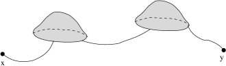
Figure 1.

We choose a generic pair of a Morse function $f\colon L\to\mathbb{R}$ and a Riemannian metric on $L$ and consider a generic almost complex structure on $M$. Denote by $C_{f}^{*}$ the Morse complex associated to $f$, graded by Morse indeces of $f$. Let $A=\mathbb{Z}_{2}[T,T^{-1}]$ be the algebra of Laurent polynomials over $\mathbb{Z}_{2}$ , where we take $\deg T=N_{L}$. Take the decomposition $A=\bigoplus_{i\in\mathbb{Z}}A^{i}$, where $A^{i}$ is the subspace of homogenous elements of degree $i$.

We define the Floer complex as $CF(L,L)=C_{f}\otimes A$, which has a natural grading coming from grading on $C_{f},A$. More specifically,

$$CF^{l}(L,L)=\bigoplus_{k\in\mathbb{Z}}C_{f}^{l-kN_{L}}(L,L)\otimes A^{kN_{L}},$$

for each $l\in\mathbb{Z}$. To define the Floer differential $d_{F}:CF(L,L)\rightarrow CF(L,L)$, we introduce auxiliary operators $\partial_{0},\partial_{1},\dots,\partial_{\nu}:C_{f}\rightarrow C_{f}$, where $\nu=\big{[}\frac{\dim L+1}{N_{L}}\big{]}$.

For every pair of critical points $x,y\in C_{f}$ denote by $\mathcal{M}_{k}(x,y)$ the moduli-space of diagrams as in Figure 1. This diagram consists of pieces of gradient trajectories of $-f$, joined by somewhere injective(see  [L]) pseudo-holomorphic discs $u_{1},u_{2},\ldots,u_{l}$ in $M$, with boundaries on $L$, such that the first piece of gradient trajectory converges to $x$, and the last piece converges to $y$, when time is reversed and such that sum of Maslov indices of the discs is $\mu(u_{1})+\mu(u_{2})+\ldots+\mu(u_{l})=kN_{L}$. Let us give a precise definition of an element of $\mathcal{M}_{k}(x,y)$. Consider a collection of somewhere injective pseudo-holomorphic discs $u_{j}\colon(D^{2},\partial D^{2})\rightarrow(M,L)$, $j=1,2,\ldots,l$, with boundaries on $L$, and a collection of trajectories

$$\gamma_{0}:(-\infty,a_{0}]\rightarrow L,\gamma_{1}:[a_{0},a_{1}]\rightarrow L,\gamma_{2}:[a_{1},a_{2}]\rightarrow L,\ldots,$$

$$\gamma_{l}:[a_{l-1},a_{l}]\rightarrow L,\gamma_{l+1}:[a_{l},+\infty)\rightarrow L,$$

where $-\infty<a_{0}<a_{1}<\ldots<a_{l}<+\infty$. Then we demand that $\gamma_{0},\gamma_{1},\ldots,\gamma_{l+1}$ are gradient trajectories for $-f$ (with respect to our Riemannian metric on $L$), namely

$$\dot{\gamma_{j}}(t)=-\nabla f(\gamma_{j}(t)),\quad j=0,1,2,\ldots,l+1,$$

with matching conditions :

$$\lim_{t\rightarrow+\infty}\gamma_{0}(t)=x,\lim_{t\rightarrow-\infty}\gamma_{l}(t)=y,$$

$$\gamma_{j}(a_{j})=u_{j+1}(-1),\quad j=0,1,\ldots,l-1,$$

$$\gamma_{j}(a_{j-1})=u_{j}(1),\quad j=1,2,\ldots,l,$$

and that the total Maslov of the collection $u_{1},u_{2},\ldots,u_{l}$ of discs is

$$\mu(u_{1})+\mu(u_{2})+\ldots+\mu(u_{l})=kN_{L}.$$

Then an element of $\mathcal{M}_{k}(x,y)$ is given by a collection

$$\{(u_{1},u_{2},\ldots,u_{l}),(\gamma_{0},\gamma_{1},\ldots,\gamma_{l})\}$$

as above, when we factorize it by its group of inner automorphisms.

For generic choice of $f$ and of almost complex structures (see  [Oh-1] for the details), $\mathcal{M}_{k}(x,y)$ is a manifold of dimension

$$\dim\mathcal{M}_{k}(x,y)=\operatorname{ind}(y)-\operatorname{ind}(x)+kN_{L}-1$$

(see  [FOOO, Oh-3]). If the dimension is $0$, $\mathcal{M}_{k}(x,y)$ is a manifold of dimension $0$ and is compact, so it is a finite collection of points. Denote in this case $n_{k}(x,y):=\sharp\mathcal{M}_{k}(x,y)(\mod 2)$. Then define

$$\partial_{k}(x)=\sum_{y\in C_{f},ind(y)-ind(x)+kN_{L}-1=0}n_{k}(x,y)y.$$

Note that $\partial_{0}$ is the usual Morse-cohomology boundary operator. We see that $d_{F}$ is not compatible with grading, since each $\partial_{i}$ acts like $\partial_{i}:C_{f}^{*}\to C_{f}^{*+1-iN_{L}}(L)$.

Let Floer differential $d_{F}:CF^{*}(L,L)\rightarrow CF^{*+1}(L,L)$ by definition equals to $d_{F}=\partial_{0}\otimes 1+\partial_{1}\otimes T+\ldots+\partial_{\nu}\otimes T^{\nu}$. Then one can show that $d_{F}$ is indeed a differential. It is well known that the homology of the complex $(CF(L,L),d_{F})$ is canonically isomorphic to the Floer cohomology of the pair $(L,L)$ (see  [B-Co-1, B-Co-2] and the references therein). Therefore we will write

$$HF^{*}(L,L)=H^{*}(CF(L,L),d_{F}).$$

Consider now the following decreasing filtration on $CF(L,L)$:

$$F^{p}CF(L,L)=\{\sum x_{i}\otimes T^{n_{i}}\mid x_{i}\in C_{f},n_{i}\geqslant p\}.$$

It is obviously compatible with $d_{F}$ (due to the monotonicity of $L$), so by a standard algebraic argument we obtain the spectral sequence $\{E_{r}^{p,q},d_{r}\}$. The following properties of it have been proved in [B]:

• $E_{0}^{p,q}=C_{f}^{p+q-pN_{L}}\otimes A^{pN_{L}}$ , $d_{0}=[\partial_{0}]\otimes 1$

• $E_{1}^{p,q}=H^{p+q-pN_{L}}(L,\mathbb{Z}_{2})\otimes A^{pN_{L}}$ , $d_{1}=[\partial_{1}]\otimes T$, where $[\partial_{1}]:H^{p+q-pN_{L}}(L,\mathbb{Z}_{2})\rightarrow H^{p+1+q-(p+1)N_{L}}(L,\mathbb{Z}_{2})$ is induced from $\partial_{1}$.

• For every $r\geq 1$, $E_{r}^{p,q}$ has the form $E_{r}^{p,q}=V_{r}^{p,q}\otimes A^{pN_{L}}$ with $d_{r}=\delta_{r}\otimes T^{r}$, where $V_{r}^{p,q}$ are vector spaces over $\mathbb{Z}_{2}$ and $\delta_{r}$ are homomorphisms $\delta_{r}:V_{r}^{p,q}\to V_{r}^{p+r,q-r+1}$ defined for every $p,q$ and satisfy $\delta_{r}\circ\delta_{r}=0$. Moreover

  $$V_{r+1}^{p,q}=\frac{\ker(\delta_{r}:V_{r}^{p,q}\to V_{r}^{p+r,q-r+1})}{\textnormal{image\,}(\delta_{r}:V_{r}^{p-r,q+r-1}\to V_{r}^{p,q})}.$$

  (For $r=0,1$ we have $V_{0}^{p,q}=C_{f}^{p+q-pN_{L}}$, $V_{1}^{p,q}=H^{p+q-pN_{L}}(L;\mathbb{Z}_{2})$.)

• $\{E_{r}^{p,q},d_{r}\}$ collapses at $\nu+1$ step, namely $d_{r}=0$ for every $r\geqslant\nu+1$, so $E_{r}^{p,q}=E_{\infty}^{p,q}$ for every $r\geqslant\nu+1$ and the sequence converges to $HF$, i.e

  $$E_{\infty}^{p,q}\cong\frac{F^{p}HF^{p+q}(L,L)}{F^{p+1}HF^{p+q}(L,L)},$$

  where $F^{p}HF(L,L)$ is the filtration on $HF(L,L)$, induced from the filtration $F^{p}CF(L,L)$.

Note that on each $E_{r}$ and $V_{r}$ we have a natural grading coming from the grading on $CF(L,L)$ and $d_{r}:E_{r}\rightarrow E_{r}$ shifts this grading by $1$. Therefore $\delta_{r}:V_{r}\to V_{r}$ shifts the grading on $V_{r}$ by $1-rN_{L}$, since the degree of $T$ is $N_{L}$. On $V_{1}$ this grading coincides with the natural grading on the cohomology ring $H^{*}(L,\mathbb{Z}_{2})$.

3.2. Quantum product on Floer cohomology

Consider generic Morse functions $f,g,h:L\rightarrow\mathbb{R}$ and denote by

$$(CF_{f},d_{F}^{f}),(CF_{g},d_{F}^{g}),(CF_{h},d_{F}^{h})$$

the corresponding Floer complexes. Then we will be able to define a ”quantum product” $\star:CF_{f}\otimes CF_{g}\rightarrow CF_{h}$, such that differentials will satisfy the following analog of the Leibnitz rule:

$$d_{F}^{h}(a\star b)=d_{F}^{f}(a)\star b+a\star d_{F}^{g}(b).$$

Moreover, this product is compatible with the filtrations on the $CF$’s in the sense that $*$ maps $F^{p}CF_{f}\otimes F^{p^{\prime}}CF_{g}$ to $F^{p+p^{\prime}}CF_{h}$.

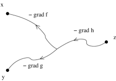
Figure 2.

Then automatically the spectral sequences become multiplicative, i.e we have products $E_{r}^{p,q}(f)\otimes E_{r}^{p^{\prime},q^{\prime}}(g)\rightarrow E_{r}^{p+p^{\prime},q+q^{\prime}}(h)$ at each stage of the spectral sequence, which are induced from $\star$, such that the differential $d_{r}$ satisfies the Leibnitz rule, according to this product, and such that the product at the $r+1$ stage comes from the product at $r$ stage. Note that in this case these products induce products $V_{r}^{p,q}(f)\otimes V_{r}^{p^{\prime},q^{\prime}}(g)\rightarrow V_{r}^{p+p^{\prime},q+q^{\prime}}(h)$, the differential $\delta_{r}:V_{r}^{p,q}\to V_{r}^{p+r,q-r+1}$ satisfies the Leibnitz rule with respect to this product and that the product on the $V_{r+1}$ is induced from the product on $V_{r}$. Then the crucial observation will be that on $V_{1}$ the induced product coincides with the usual cup-product on $H^{*}(L;\mathbb{Z}_{2})$, so the next products on the $V_{r}$ are induced from this cup product, therefore the quantum effects are lost for $r\geqslant 1$. Now let us describe the operation $\star:F^{p}CF_{f}\otimes F^{p^{\prime}}CF_{g}\rightarrow F^{p+p^{\prime}}CF_{h}$. To do this, let us introduce operations $m_{l}:C_{f}\otimes C_{g}\rightarrow C_{h}$ (for a more general introduction of such an operations see  [BC, FOOO]). The operation $m_{0}$ is the usual product on the Morse complexes of $f,g,h$. Let us recall its definition. For every triple of generators $x\in C_{f},y\in C_{g},z\in C_{h}$, denote by $\mathcal{M}_{0}(x,y;z)$ the moduli-space of diagrams as in Figure 2. This diagram is given by trajectories $\gamma_{f}:[0,+\infty)\rightarrow L,\gamma_{g}:[0,+\infty)\rightarrow L,\gamma_{h}:(-\infty,0]\rightarrow L,$ such that

$$\dot{\gamma_{f}}(t)=-\nabla f(\gamma_{f}(t)),\quad\dot{\gamma_{g}}(t)=-\nabla g(\gamma_{g}(t)),\quad\dot{\gamma_{h}}(t)=-\nabla h(\gamma_{h}(t)),$$

and

$$\lim_{t\rightarrow+\infty}\gamma_{f}(t)=x,\quad\lim_{t\rightarrow+\infty}\gamma_{g}(t)=y,\quad\lim_{t\rightarrow-\infty}\gamma_{h}(t)=z,$$

$$\gamma_{f}(0)=\gamma_{g}(0)=\gamma_{h}(0).$$

Then by our assumption that $f,g,h$ is a generic triple of Morse functions, we get that $\mathcal{M}_{0}(x,y;z)$ is a manifold, and its dimension is given by $\operatorname{ind}_{z}h-\operatorname{ind}_{x}f-\operatorname{ind}_{y}g$. Moreover, when $\operatorname{ind}_{z}h-\operatorname{ind}_{x}f-\operatorname{ind}_{y}g=0$, $\mathcal{M}_{0}(x,y;z)$ is a zero-dimensional compact manifold, hence it consists of a finite number of points. For the case of $\operatorname{ind}_{z}h-\operatorname{ind}_{x}f-\operatorname{ind}_{y}g=0$ we set $n_{0}(x,y;z):=\sharp\mathcal{M}_{0}(x,y;z)(\mod 2)$. Now we define

$$m_{0}(x,y):=\sum_{z\in C_{h},\operatorname{ind}_{z}h-\operatorname{ind}_{x}f-\operatorname{ind}_{y}g=0}n_{0}(x,y;z)z.$$

This is the classical cup product $C_{f}^{i}\otimes C_{g}^{j}\rightarrow C_{h}^{i+j}$, and so the classical Morse differential satisfies the Leibnitz rule and induces the classical cup-product on cohomology $H^{*}(L;\mathbb{Z}_{2})$. The further operations $m_{l}$ for $l\geqslant 1$ will use quantum contributions.

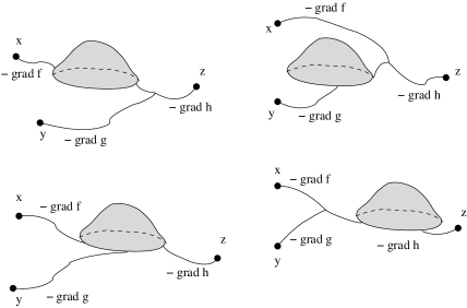
Figure 3.

Before defining the general $m_{l}$, let us first describe $m_{1}$. For a triple of critical points $x\in C_{f},y\in C_{g},z\in C_{h}$, we define the space $\mathcal{M}_{1}(x,y;z)$ to be the moduli-space of diagrams as in Figure 3, where ”black lines” are gradient trajectories of $f,g,h$ respectively and the ”discs” are pseudo-holomorphic somewhere injective discs with boundaries on $L$ and Maslov indices equal to $N_{L}$. Let us describe the first and the second diagram from the Figure 3. The first diagram is given by a collection

$$(u,\gamma_{f1},\gamma_{f2},\gamma_{g},\gamma_{h}),$$

where $u:(D^{2},S^{1})\rightarrow(M,L)$ is a pseudo-holomorphic disc in $M$ with boundary on $L$ and

$$\gamma_{f1}:[0,+\infty)\rightarrow L,\gamma_{f2}:[0,a]\rightarrow L,\gamma_{g}:[0,+\infty)\rightarrow L,\gamma_{h}:(-\infty,0]\rightarrow L,$$

where $0<a\in\mathbb{R}$, such that

$$\dot{\gamma}_{f1}(t)=-\nabla f(\gamma_{f1}(t)),\quad\dot{\gamma}_{f2}(t)=-\nabla f(\gamma_{f2}(t)),\quad\dot{\gamma_{g}}(t)=-\nabla g(\gamma_{g}(t)),$$

$$\dot{\gamma_{h}}(t)=-\nabla h(\gamma_{h}(t)),$$

$$\lim_{t\rightarrow+\infty}\gamma_{f1}(t)=x,\quad\lim_{t\rightarrow+\infty}\gamma_{g}(t)=y,\quad\lim_{t\rightarrow-\infty}\gamma_{h}(t)=z,$$

$$\gamma_{f2}(0)=\gamma_{g}(0)=\gamma_{h}(0),\quad\gamma_{f1}(0)=u(-1),\quad\gamma_{f2}(a)=u(1).$$

The second diagram is given by a collection $(u,\gamma_{f},\gamma_{g},\gamma_{h})$, where $u:(D^{2},S^{1})\rightarrow(M,L)$ is a somewhere injective pseudo-holomorphic disc in $M$, with boundary on $L$ and

$$\gamma_{f}:[0,+\infty)\rightarrow L,\gamma_{g}:[0,+\infty)\rightarrow L,\gamma_{h}:(-\infty,0]\rightarrow L,$$

such that

$$\dot{\gamma_{f}}(t)=-\nabla f(\gamma_{f}(t)),\quad\dot{\gamma_{g}}(t)=-\nabla g(\gamma_{g}(t)),\quad\dot{\gamma_{h}}(t)=-\nabla h(\gamma_{h}(t)),$$

$$\lim_{t\rightarrow+\infty}\gamma_{f}(t)=x,\quad\lim_{t\rightarrow+\infty}\gamma_{g}(t)=y,\quad\lim_{t\rightarrow-\infty}\gamma_{h}(t)=z,$$

$$\gamma_{f}(0)=u(1),\quad\gamma_{g}(0)=u(i),\quad\gamma_{h}(0)=u(-1).$$

The other diagrams from the picture have analogous definitions. For generic choices of $f,g,h$ and of almost complex structures, $\mathcal{M}_{1}(x,y;z)$ is a manifold of dimension $\operatorname{ind}_{z}h-\operatorname{ind}_{x}f-\operatorname{ind}_{y}g+N_{L}$. As before, if $\dim\mathcal{M}_{1}(x,y;z)=0$, it is a zero-dimensional compact manifold, hence it is a finite collection of points and we set $n_{1}(x,y;z):=\sharp\mathcal{M}_{1}(x,y;z)(\mod 2)$. Now we define

$$m_{1}(x,y):=\sum_{z\in C_{h},\operatorname{ind}_{z}h-\operatorname{ind}_{x}f-\operatorname{ind}_{y}g+N_{L}=0}n_{1}(x,y;z)z.$$

For defining $m_{l}$ for general $l$ we introduce a manifold $\mathcal{M}_{l}(x,y;z)$ for $x\in C_{f},y\in C_{g},z\in C_{h}$. Its points are diagrams like in Figure 3, but instead they include several somewhere injective discs with total Maslov index $lN_{L}$. In general these diagrams are of two types, as in Figures 4 and  5.

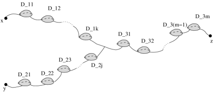
Figure 4.

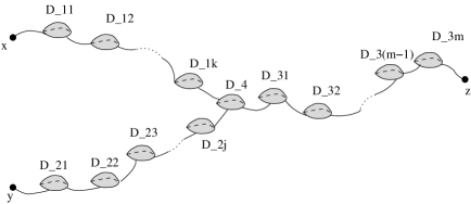
Figure 5.

In Figure 4, $D_{11},D_{12},\ldots,D_{1k}$ are somewhere injective pseudo-holomorphic discs with boundaries on $L$, which connect pieces of gradient trajectories of $f$, $D_{21},D_{22},\ldots,D_{2j}$ - of $g$, and $D_{31},D_{32},\ldots,D_{3m}$ - on $h$, such that $k,j,m\geqslant 0$ and total Maslov index

$$\sum_{i,j}\mu(D_{ij})=lN_{L}.$$

In Figure 5 in addition we have a disc $D_{4}$ in the middle, with gradient trajectory of $h$ going into and gradient trajectories of $f,g$ going out of its boundary, and as before the total Maslov index is

$$\mu(D_{4})+\sum_{i,j}\mu(D_{ij})=lN_{L}.$$

We will denote by $\mathcal{\overline{M}}_{l}^{kjm}(x,y;z)$ the space of diagrams as in Figure 4 and by $\mathcal{\widetilde{M}}_{l}^{kjm}(x,y;z)$ the space of diagrams as in Figure 5. Denote also $\mathcal{\overline{M}}_{l}(x,y;z)=\bigcup_{k,j,m}\mathcal{\overline{M}}_{l}^{kjm}(x,y;z)$, $\mathcal{\widetilde{M}}_{l}(x,y;z)=\bigcup_{k,j,m}\mathcal{\widetilde{M}}_{l}^{kjm}(x,y;z)$. We have that

$$\mathcal{M}_{l}(x,y;z)=\mathcal{\overline{M}}_{l}(x,y;z)\cup\mathcal{\widetilde{M}}_{l}(x,y;z)$$

and $\dim(\mathcal{M}_{l}(x,y;z))=\operatorname{ind}_{z}h-\operatorname{ind}_{x}f-\operatorname{ind}_{y}g+lN_{L}$. Then, as before, in the case of $\operatorname{ind}_{z}h-\operatorname{ind}_{x}f-\operatorname{ind}_{y}g+lN_{L}=0$, we have that $\mathcal{M}_{l}(x,y;z)$ is a finite collection of points and we set $n_{l}(x,y;z):=\sharp\mathcal{M}_{l}(x,y;z)$ in this case. Then, as usual, we define

$$m_{l}(x,y):=\sum_{z\in C_{h},\operatorname{ind}_{z}h-\operatorname{ind}_{x}f-\operatorname{ind}_{y}g+lN_{L}=0}n_{l}(x,y;z)z$$

for generators $x\in C_{f},y\in C_{g}$.

Now we can define the quantum product $\star:F^{p}CF_{f}\otimes F^{p^{\prime}}CF_{g}\rightarrow F^{p+p^{\prime}}CF_{h}$ by $x\star y=m_{0}(x,y)\otimes 1+m_{1}(x,y)\otimes T+m_{2}(x,y)\otimes T^{2}+\ldots$ for $x\in C_{f},y\in C_{g}$, and then naturally extend it to a map $CF^{i}_{f}\otimes CF^{j}_{g}\rightarrow CF^{i+j}_{h}$. Note that the filtrations on $CF_{f},CF_{g},CF_{h}$ are compatible with this map, i.e the image of $F^{p}CF_{f}\otimes F^{p^{\prime}}CF_{g}$ is in $F^{p+p^{\prime}}CF_{h}$. This sum is finite, because $\operatorname{ind}_{z}h-\operatorname{ind}_{x}f-\operatorname{ind}_{y}g+lN_{L}=0$, hence $l=(-\operatorname{ind}_{z}h+\operatorname{ind}_{x}f+\operatorname{ind}_{y}g)/N_{L}\leqslant 2n/N_{L}$. The main goal is now to prove the following theorems.

Theorem 4.

The differentials $d_{F}^{f},d_{F}^{g},d_{F}^{h}$ satisfy the Leibnitz rule with respect to the product $\star$

$$d_{F}^{h}(a\star b)=d_{F}^{f}(a)\star b+a\star d_{F}^{g}(b),$$

for every $a\in CF_{f},b\in CF_{g}$.

Theorem 5.

The product on $V_{1}$, induced from $\star$, coincides with the classical cup-product on $H^{*}(L;\mathbb{Z}_{2})$.

4. Existence and properties of the quantum product - proofs

Proof of Theorem 4.

The main idea of the proof is similar to the analogous statement in classical Morse theory, for a standard Morse differential and a product on the Morse complex. In what follows we have to find a compactification of the manifolds $\mathcal{\overline{M}}_{l}(x,y;z)$ and $\mathcal{\widetilde{M}}_{l}(x,y;z)$. We are mostly interested in the components of the boundary of codimension $1$. A point of the compactification of $\mathcal{M}_{l}(x,y;z)$ is a diagram, consisting of several pseudo-holomorphic discs with boundaries on $L$, spheres, critical points of $f,g,h$ and pieces of gradient trajectories of $f,g,h$ between them. Let us describe what can happen when we pass to the limit of a sequence of elements of $\mathcal{M}_{l}(x,y;z)$. First, some of the gradient trajectories of $f,g$ or $h$ can ”brake” and new critical points of $f,g,h$ can appear in the diagram. Second, some of the pieces of the gradient trajectories can ”shrink” to a point, such that we will obtain two touching discs or one disc containing a critical point. Also looking on $\mathcal{\overline{M}}_{l}(x,y;z)$, the piece of gradient trajectory containing the ”middle point” can shrink to a point, so we will get a disc containing this ”middle point”. It can also happen that some of the discs split to a tree of discs and also some of the discs can bubble a sphere. The last thing that can happen is that for some pieces of trajectories which have endpoints on a disc, their endpoints on that disc converge one to another and become a single point. All these degenerations can happen simultaneously. However, when one looks on the codimension-$1$ part of the boundary of $\mathcal{M}_{l}(x,y;z)$, only one of this degenerations can happen, moreover when we have the case of breaking of some trajectory, it can brake only at one point and this can happen only for one trajectory. Also, when we have ”shrinking” of some trajectory, only one trajectory can shrink to a point. Thirdly, when we have splitting of a disc to discs, then only one disc can split and only to two discs, and bubbling of spheres always has co-dimension $\geqslant 2$. Finally, when endpoints of some trajectories, lying on the boundary of some disc, become one point, we always have codimension $\geqslant 2$, except for the case when it is in $\mathcal{\widetilde{M}}_{l}(x,y;z)$, and two of the trajectories which end on the boundary of the ”middle disc” in the limit have the same end on this boundary.

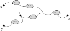
Figure 6.

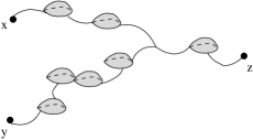
Figure 7.

Therefore, when we are looking only at the codimension $1$ part of $\mathcal{M}_{l}(x,y;z)$, only the following cases can happen:

For $\mathcal{\overline{M}}_{l}(x,y;z)$ we can obtain:

$a$) One trajectory ”brakes” and we obtain a situation as in Figure  6, when a new critical point $t$ appears ( this can happen with gradient trajectories of $f,g,h$).

$b$) Two neighboring discs in the chain become ”touching” and the trajectory which joins them collapses into a point, as in Figure 7.

$c$) The last disc from the chain of discs of $g$, for example, comes closer and closer to the ”middle point”, where gradient trajectories of $f,g,h$ meet, until the trajectory which connects it to this ”middle point” collapses to a point ( as in Figure 8 ).

$d$) One of the discs splits to the union of two touching discs (Figure 9).

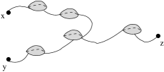
Figure 8.

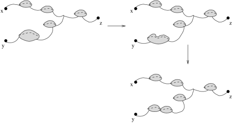
Figure 9.

Denote by

$$\mathcal{M}^{a}_{l}(x,y;z),\mathcal{M}^{b}_{l}(x,y;z),\mathcal{M}^{c}_{l}(x,y;z),\mathcal{M}^{d}_{l}(x,y;z)$$

the manifolds of diagrams of types $a,b,c,d$ respectively.

Now addressing to the co-dimension $1$ compactification of $\mathcal{\widetilde{M}}_{l}(x,y;z)$, we see that the following cases are possible:

$e$) One trajectory ”brakes” and we obtain a situation as in Figure  10.

$f$) Two neighboring discs in the chain come close and the trajectory which joins them collapses to a point, or the middle disc comes close to some neighboring disc as in Figure 11.

$g$) One of the discs splits to a union of two touching discs (and we again obtain a situation as in Figure 11).

$h$) Two trajectories touching the middle disc converge to trajectories which touch the middle disc in the same point. We obtain again Figure 8.

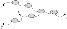
Figure 10.

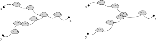
Figure 11.

As before, we denote by

$$\mathcal{M}^{e}_{l}(x,y;z),\mathcal{M}^{f}_{l}(x,y;z),\mathcal{M}^{g}_{l}(x,y;z),\mathcal{M}^{h}_{l}(x,y;z)$$

the manifolds of the situations $e,f,g,h$ respectively. Note that

$$(*)\begin{cases}\mathcal{M}^{c}_{l}(x,y;z)=\mathcal{M}^{h}_{l}(x,y;z)\\ \mathcal{M}^{b}_{l}(x,y;z)=\mathcal{M}^{d}_{l}(x,y;z)\\ \mathcal{M}^{f}_{l}(x,y;z)=\mathcal{M}^{g}_{l}(x,y;z)\end{cases}$$

Now let us see how this can be applied to prove the Leibnitz rule. Let us first write what it means. Taking $x\in C_{f},y\in C_{g}$, we have

$$d_{F}^{h}(x\star y)=d_{F}^{h}(\sum_{i\geqslant 0}m_{i}(x,y)\otimes T^{i})=\sum_{i,j\geqslant 0}\partial_{j}(m_{i}(x,y))\otimes T^{j+i}.$$

Similarly,

$$d_{F}^{f}(x)\star y=\sum_{j,i\geqslant 0}m_{i}(\partial_{j}x,y)\otimes T^{j+i}$$

and

$$x\star d_{F}^{g}(y)=\sum_{j,i\geqslant 0}m_{i}(x,\partial_{j}y)\otimes T^{j+i}.$$

Therefore, we are left with proving that for every $l$,

$$\sum_{i,j\geqslant 0,i+j=l}\partial_{j}(m_{i}(x,y))=\sum_{i,j\geqslant 0,i+j=l}m_{i}(\partial_{j}x,y)+\sum_{i,j\geqslant 0,i+j=l}m_{i}(x,\partial_{j}y).$$

This means that we have to show that for every choice of generators $x\in C_{f},y\in C_{g},z\in C_{h}$ with $\operatorname{ind}(z)=\operatorname{ind}(x)+\operatorname{ind}(y)+lN_{L}+1$, the total number of configurations in $\mathcal{M}^{a}_{l}(x,y;z)\cup\mathcal{M}^{e}_{l}(x,y;z)$ is even. For this consider the space $\mathcal{M}_{l}(x,y;z)$. It is a $1$-dimensional manifold, therefore its boundary consists of an even number of points. On the other hand, from a gluing argument (see [FO, FOOO, MS, S]) it follows that this boundary is the union of

$$\mathcal{M}^{a}_{l}(x,y;z),\mathcal{M}^{b}_{l}(x,y;z),\mathcal{M}^{c}_{l}(x,y;z),\mathcal{M}^{d}_{l}(x,y;z),$$

$$\mathcal{M}^{e}_{l}(x,y;z),\mathcal{M}^{f}_{l}(x,y;z),\mathcal{M}^{g}_{l}(x,y;z),\mathcal{M}^{h}_{l}(x,y;z)$$

(because in our case $\dim\mathcal{M}_{l}(x,y;z)=1$, so in a generic situation the part of the boundary of $\mathcal{M}_{l}(x,y;z)$ of co-dimension bigger than $1$ must be of dimension less than $0$, so it is an empty set). Now, $(*)$ shows that modulo $2$, the total number of points on the boundary of $\mathcal{M}_{l}(x,y;z)$ is equal to $\sharp\mathcal{M}^{a}_{l}(x,y;z)+\sharp\mathcal{M}^{f}_{l}(x,y;z)$ and is even. This proves Theorem 4. ∎

Remark.

In several places we have applied the dimension formula $\dim\mathcal{M}(A,J)=n+\mu(A)$, where $\mathcal{M}(A,J)$ is a manifold of $J$-holomorphic maps $u\colon(D^{2},\partial D^{2})\rightarrow(M,L)$ with $[u]=A\in\pi_{2}(M,L)$, in order to show that certain configurations of gradient trajectories and pseudo-holomorphic discs cannot appear for generic choice of $J$ ( because of negative dimension ). However, this dimension formula is based on the transversality argument ( see [MS] ) which requires somewhere injectivity of the $J$-holomorphic discs. To solve this problem we use work of Kwon, Oh and of Lazzarini ( see [K-O, L] ). More precisely, suppose we have such a configuration and some pseudo-holomorphic disc $u:(D,\partial D)\rightarrow(M,L)$ participated in it is not somewhere injective. Then we can decompose it to a union of almost everywhere injective discs $u_{1},u_{2},\ldots,u_{k}$ with multiplicities $m_{1},m_{2},\ldots,m_{k}$ respectively, such that there exists $m_{j}>1$ ( see [K-O, L] for the precise details of this decomposition ). This decomposition preserves the relative homology class, namely

$$[u]=m_{1}[u_{1}]+m_{2}[u_{2}]+\ldots+m_{k}[u_{k}]\in H_{2}(M,L),$$

however, when we look on this configuration when we take all the discs $u_{j}$ with multiplicity $1$, then it’s total area and hence a total Maslov class is strictly smaller than of the original configuration, therefore by a usual dimension count we obtain that such a configuration has negative dimension and hence cannot appear in a generic situation, therefore the original configuration also cannot appear. See  [B-Co-1] for more details on such arguments.

Proof of Theorem 5.

First look at the induced product on the level $E_{0}$. Let us show that it coincides with the classical product on the Morse complex. From the standard construction of the spectral sequence we have that

$$E_{0}^{p,q}(f)=F^{p}CF_{f}^{p+q}/F^{p+1}CF_{f}^{p+q}\cong V_{0}^{p,q}(f)\otimes A^{pN_{L}},$$

$$E_{0}^{p^{\prime},q^{\prime}}(g)=F^{p^{\prime}}CF_{g}^{p^{\prime}+q^{\prime}}/F^{p^{\prime}+1}CF_{g}^{p^{\prime}+q^{\prime}}\cong V_{0}^{p^{\prime},q^{\prime}}(g)\otimes A^{p^{\prime}N_{L}},$$

where $V_{0}^{p,q}(f)=C_{f}^{p+q-pN_{L}}$, $V_{0}^{p^{\prime},q^{\prime}}(g)=C_{g}^{p^{\prime}+q^{\prime}-p^{\prime}N_{L}}$. Now take $\alpha\in V_{0}^{p,q}(f)$, $\beta\in V_{0}^{p^{\prime},q^{\prime}}(g)$. Now, we can take $\overline{\alpha}:=\alpha\otimes T^{p}\in F^{p}CF_{f}^{p+q}$, $\overline{\beta}:=\beta\otimes T^{p^{\prime}}\in F^{p^{\prime}}CF_{g}^{p^{\prime}+q^{\prime}}$ as a pre-images of $\alpha\otimes T^{p}\in E_{0}^{p,q}(f)$, $\beta\otimes T^{p^{\prime}}\in E_{0}^{p^{\prime},q^{\prime}}(g)$ under natural projections $F^{p}CF_{f}^{p+q}\rightarrow E_{0}^{p,q}(f)$, $F^{p^{\prime}}CF_{g}^{p^{\prime}+q^{\prime}}\rightarrow E_{0}^{p^{\prime},q^{\prime}}(g)$ respectively. Then, by definition of the product $\star$,

$$\overline{\alpha}\star\overline{\beta}=m_{0}(\alpha,\beta)\otimes T^{p+p^{\prime}}+m_{1}(\alpha,\beta)\otimes T^{p+p^{\prime}+1}+$$

$$+m_{2}(\alpha,\beta)\otimes T^{p+p^{\prime}+2}+\ldots\in F^{p+p^{\prime}}CF_{h}^{q+q^{\prime}},$$

and so the induced product of $\alpha\otimes T^{p}\in E_{0}^{p,q}(f)$, $\beta\otimes T^{p^{\prime}}\in E_{0}^{p^{\prime},q^{\prime}}(g)$ is the image of $\overline{\alpha}\star\overline{\beta}\in C_{h}^{p+p^{\prime}+q+q^{\prime}-pN_{L}-p^{\prime}N_{L}}$ under the natural projection $F^{p+p^{\prime}}CF_{h}^{p+p^{\prime}+q+q^{\prime}}\rightarrow E_{0}^{p+p^{\prime},q+q^{\prime}}(h)$, which is $m_{0}(\alpha,\beta)\otimes T^{p+p^{\prime}}$. Therefore the induced product of $\alpha\in V_{0}^{p,q}(f)$, $\beta\in V_{0}^{p^{\prime},q^{\prime}}(g)$ is $m_{0}(\alpha,\beta)\in V_{0}^{p+p^{\prime},q+q^{\prime}}(h)$, which is the classical product in the Morse complex. Note also that the differential $\delta_{0}:V_{0}^{p,q}\to V_{0}^{p,q+1}$ coincides with classical Morse differential, therefore the induced product on $V_{1}=H(V_{0},\delta_{0})$ is the classical cup-product. ∎

5. Basic notions of symplectic topology in terms of Lagrangian Floer theory.

In this section we summarize some relevant notions from symplectic topology used in the article.

5.1. Tame symplectic manifold

A symplectic manifold $(M,\omega)$ is called tame if there exists an almost complex structure $J$, such that the bilinear form $g_{\omega,J}(\cdot,\cdot)=\omega(\cdot,J\cdot)$ is a Riemmanian metric on $M$, and moreover the Riemmanian manifold $(M,g_{\omega,J})$ is geometrically bounded (i.e. its sectional curvature is bounded above and the injectivity radius is bounded below). See  [A-L-P, Gr] for more details and the relevance of this condition for the theory of pseudo-holomorphic curves.

5.2. The Maslov class

The Maslov class is a homomorphism $\mu_{L}:\pi_{2}(M,L)\rightarrow\mathbb{Z}$, associated to a Lagrangian submanifold $L\subset(M,\omega)$ . To describe it, we start with the linear case. Consider the space $\mathbb{R}^{2n}\cong\mathbb{C}^{n}$ with standard symplectic structure. Denote by $\mathcal{L}(n)$ the set of all Lagrangian linear subspaces of $\mathbb{R}^{2n}$. The unitary group $U(n)$ acts transitively on $\mathcal{L}(n)$ such that a stabilizer of Lagrangian subspace $\mathbb{R}^{n}=\{y_{1}=\ldots=y_{n}=0\}\subset\mathbb{C}^{n}$ is the orthogonal group $O(n)\subset U(n)$. So $\mathcal{L}(n)$ is homeomorphic to the quotient $U(n)/O(n)$. On $U(n)/O(n)$ we have well-defined map $det^{2}:U(n)/O(n)\rightarrow S^{1}\subset\mathbb{C}$, hence we obtain a map $\mathcal{L}(n)\rightarrow S^{1}$. The corresponding homomorphism $\mu:\pi_{1}(\mathcal{L}(n))\rightarrow\mathbb{Z}$ is called the Maslov index. It can be verified that it is an isomorphism.

Now, consider a symplectic manifold $(M,\omega)$ and a Lagrangian submanifold $L\subset M$. Take a disc in $M$ with boundary lying on $L$: $u:(D,\partial D)\rightarrow(M,L)$. We obtain the following diagram of vector bundles:

$$\begin{array}[]{clcr}u^{*}T(M)&\supset&u^{*}T(L)\\ \downarrow&&\downarrow\\ D&&\partial D\end{array}$$

Over each point on the disc $D$ we have a symplectic linear space and for every point on the boundary $\partial D$ we have a Lagrangian linear subspace of the corresponding linear symplectic space. Now, we can symplectically trivialize the bundle $u^{*}T(M)\rightarrow D$, and as a result we will get a loop of Lagrangians in $\mathbb{R}^{2n}$, $\gamma:S^{1}\rightarrow\mathcal{L}(n)$. Applying to this loop the Maslov index, we get the Maslov class evaluated on $D$, namely, we define $\mu_{L}(D)=\mu(\gamma)$. It can be shown that this definition does not depend on the trivialization, and actually depends only on $[D]\in\pi_{2}(M,L)$. Given a Lagrangian submanifold $L\subset(M,\omega)$ we denote by $N_{L}$ the positive generator of the image $\mu_{L}(\pi_{2}(M,L))\subset\mathbb{Z}$. We shall refer to $N_{L}$ as the minimal Maslov number of $L$.

5.3. Symplectic area class

This is a homomorphism $\omega:\pi_{2}(M,L)\rightarrow\mathbb{R}$ which computes the symplectic area of a disc: if we have a representative $\alpha=[\varphi:(D,\partial D)\rightarrow(M,L)]\in\pi_{2}(M,L)$ , we define $\omega(\alpha):=\int_{D}(\varphi^{*}\omega)$. Also here it can be shown that the symplectic area class $\omega(\alpha)$ depends only on $\alpha\in\pi_{2}(M,L)$.

5.4. Monotone symplectic manifolds

Let $(M,\omega)$ be a symplectic manifold. Denote by $c_{1}\in H^{2}(M;\mathbb{R})$ the first Chern class of the tangent bundle $T(M)$ viewed as a complex vector bundle (where the complex structure on $T(M)$ is taken to be any almost complex structure tamed by $\omega$). We say that $(M,\omega)$ is a monotone symplectic manifold if there exists a positive real number $\lambda>0$ such that $[\omega]=\lambda c_{1}$ . Given a Lagrangian submanifold $L\subset(M,\omega)$, we have two homomorphisms: $\mu_{L}:\pi_{2}(M,L)\rightarrow\mathbb{Z}$, and $\omega:\pi_{2}(M,L)\rightarrow\mathbb{R}$. We say that $L$ is monotone, if these two homomorphisms $\mu_{L},\omega$ are proportional by some positive constant, that is, there exists a constant $\lambda\in\mathbb{R},\lambda>0$ , such that for every $\alpha\in\pi_{2}(M,L)$ we have $\mu_{L}(\alpha)=\lambda\omega(\alpha)$.

Acknowledgments

I would like to thank my supervisor Paul Biran for his help and attention he gave to me. I am grateful to Felix Schlenk for his comments and for helping me to improve the quality of the exposition. Also I am grateful to Leonid Polterovich, Alex Ivri and Laurent Lazzarini for useful comments.

References

- [A] M. Audin, Fibrés normaux d’immersions en dimension double, points doubles d’immersions lagragiennes et plongements totalement réels. Comment. Math. Helv. 63 (1988), no. 4, 593–623.
- [A-L-P] M. Audin, F. Lalonde and L. Polterovich, Symplectic rigidity: Lagrangian submanifolds. In Holomorphic curves in symplectic geometry. Edited by M. Audin and J. Lafontaine. Progress in Mathematics, 117. Birkhäuser Verlag, Basel, 1994.
- [BC] M. Betz, R. L. Cohen Moduli spaces of graphs and cohomology operations. Turkish Jour. of Math. 18 (1994), 23–41.
-
[B]
P. Biran, Lagrangian
non-intersections., to appear in GAFA,
can be downloaded at
http://arxiv.org/abs/math.SG/0412110 - [B-Ci] P. Biran, K. Cieliebak, Lagrangian embeddings into subcritical Stein manifolds. Israel J. Math. 127 (2002), 221–244.
- [B-Co-1] P. Biran, O. Cornea, Quantum Structures for Lagrangian Submanifolds. Preprint, can be downloaded at http://front.math.ucdavis.edu/0708.4221
- [B-Co-2] P. Biran, O. Cornea, Rigidity and uniruling for Lagrangian submanifolds. Preprint, can be downloaded at http://front.math.ucdavis.edu/0808.2440
- [B-Co-3] P. Biran, O. Cornea, Lagrangian Quantum Homology. Preprint, can be downloaded at http://front.math.ucdavis.edu/0808.3989
- [Ch] Yu. Chekanov, Lagrangian torii in a symplectic vector space and global symplectomorphisms. Math. Zeit. 223 (1996), 547–559.
-
[CL]
O.Cornea,F.Lalonde, Cluster Homology.
Manuscript, can be downloaded at
http://arxiv.org/abs/math.SG/0508345 - [E-P] Y.Eliashberg, L.Polterovich, The Problem of Lagrangian Knots in Four-Manifolds. Geometric Topology. Proceedings of the 1993 Georgia International Topology Conference (W.H.Kazez, ed.), International Press, 313-327 (1997).
- [FO] K. Fukaya and Y. G. Oh, Zero-loop open strings in the cotangent bundle and Morse homotopy. Asian J. Math. 1 (1997) no. 1, 96-180
-
[FOOO]
K. Fukaya, Y.-G. Oh, H. Ohta, K. Ono, Lagrangian intersection Floer theory-anomaly and obstruction.
Manuscript, can be downloaded at
http://www.math.kyoto-u.ac.jp/%7Efukaya/fukaya.html - [Gr] M. Gromov, Pseudoholomorphic curves in symplectic manifolds. Invent. Math. 82 (1985), no. 2, 307–347.
- [K-O] D. Kwon, Y.-G. Oh, Structure of the image of (pseudo)-holomorphic discs with totally real boundary condition. Comm. Anal. Geom. 8 (2000), no. 1, 31–82.
- [L] L. Lazzarini, Existence of a somewhere injective pseudo-holomorphic disc. Geom. Funct. Anal. 10 (2000), no. 4, 829–862.
- [Li] W. Li, Lagrangian embedding, Maslov indexes and Integer graded symplectic Floer cohomology. Can be downloaded at http://arxiv.org/abs/dg-ga/9602009
- [MS] D.McDuff,D.Salamon, J-holomorphic curves and symplectic topology. American Mathematical Society Colloquium Publications, vol.52, American Mathematical Society, Providence, RI, 2004.
- [Oh-1] Y.-G. Oh, Floer cohomology of Lagrangian intersections and pseudo-holomorphic disks. I. Comm. Pure Appl. Math. 46 (1993), no. 7, 949–993.
- [Oh-2] Y.-G. Oh, Floer cohomology, spectral sequences, and the Maslov class of Lagrangian embeddings. Internat. Math. Res. Notices 1996, no. 7, 305–346.
- [Oh-3] Y.-G. Oh, Relative Floer and quantum cohomology and the symplectic topology of Lagrangian submanifolds. Contact and symplectic geometry (Cambridge, 1994), 201–267, Publ. Newton Inst., 8, Cambridge Univ. Press, Cambridge, 1996.
- [P] L. Polterovich, Monotone Lagrange submanifolds of linear spaces and the Maslov class in cotangent bundles. Math. Z. 207 (1991), no. 2, 217–222.
-
[S]
P. Seidel, Fukaya categories and
Picard-Lefschetz theory. Manuscript, can be downloaded at
http://www.math.uchicago.edu/ seidel/done.pdf - [V-1] C. Viterbo, A new obstruction to embedding Lagrangian tori. Invent. Math. 100 (1990), no. 2, 301–320.
- [V-2] C. Viterbo, Functors and computations in Floer homology with applications. I. Geom. Funct. Anal. 9 (1999), no. 5, 985–1033.