Geometry of planar log-fronts

1 Introduction

1.1 Frozen boundaries

Given two polynomials $P(z,w)$ and $Q(z,w)$, one can study solutions of the system

$$\begin{cases}P(z,w)=0\,,\\ Q(e^{-x}z,e^{-y}w)=0\,.\end{cases}$$ (1)

as a function of a point $(x,y)\in\mathbb{R}^{2}$. A solution $z(x,y)$ and $w(x,y)$ of (1) solves a first order quasilinear PDE

$$\frac{z_{x}}{z}+\frac{w_{y}}{w}=1\,,\quad P(z,w)=0\,,$$

which is closely related to the complex Burgers equation and arises in the theory of random surfaces, see [13]. The singularities of $z(x,y)$ and $w(x,y)$ occur when (1) has a multiple root, that is, when the two curves in (1) are tangent. In the random surface context, this marks the boundary between order (e.g. crystalline facet) and disorder, called frozen boundary.

For example, let $P$ and $Q$ define rational curves in ${\mathbb{R}}{\mathbb{P}}^{2}$ of degree $2$ and $4$, respectively, positioned with respect to the coordinate axes of ${\mathbb{R}}{\mathbb{P}}^{2}$ as illustrated in Figure 1.

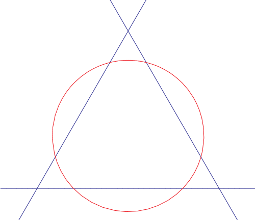
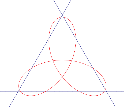
Figure 1: Curves $P$ and $Q$ for the frozen boundary in Figure 2

Points where $P$ and $Q$ intersect the axes may be fixed so that the frozen boundary will be inscribed in a hexagon as illustrated in Figure 2.

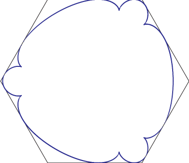
Figure 2: An example of frozen boundary

The probabilistic meaning of this curve is the following.

The well-known arctic circle theorem of Cohn, Larsen, and Propp [5] states that the limit shape of a typical 3D partition contained in a cube has a frozen boundary which is a circle. More precisely, projected in the $(1,1,1)$-direction, the cube becomes a hexagon and the $(1,1,1)$-projection of the frozen boundary is an inscribed circle. Now suppose we additionally weight each 3D partition $\pi$ by a weight which a product over all boxes

$$\textup{\char 114}=(i,j,k)\in\mathbb{Z}^{3}$$

in $\pi$ of some periodic function of $i-j$ and $j-k$. If the period equals $2$, the frozen boundary will look as in Figure 2. The coefficients of the curve $P$ are obtained from the periodic weights, while the coefficients of $Q$ are fixed by boundary conditions. See [13] for a detailed discussion of this procedure in general.

The geometry and, especially, the singularities of frozen boundaries are of considerable interest. Note that these are curves of some complexity: in our current example frozen boundary has degree $28$ and genus $27$.

1.2 Log-front

This motivates the following definition. Given two curves $P,Q\subset(\mathbb{C}^{\times})^{2}$, consider

$$R=\left\{(a,b)\,\big{|}\,\textup{$\tau_{a,b}\cdot Q$ is tangent to $P$}\right\}\subset(\mathbb{C}^{\times})^{2}$$ (2)

where

$$\tau_{a,b}:(\mathbb{C}^{\times})^{2}\to(\mathbb{C}^{\times})^{2}$$

it the dilation $(z,w)\mapsto(az,bw)$ and tangency at a singular point means that for some branches of the two curves in question their unique tangent lines coincide. For simplicity, we assume that tangency occurs only at isolated points, that is, no component of $P$ is a dilate of a component of $Q$.

We call the curve $R$ the log-front of $P$ and $Q$. The reason for such name will be explained below. We will denote the construction (2) by

$$R=P\div Q\,.$$

The obvious property

$$Q\div P=R(a^{-1},b^{-1})$$

and (4) below justify such notation.

Clearly, $R$ is an algebraic curve. Various ways to compute its equation $R(a,b)=0$ will be discussed in Section 3.1. The frozen boundary from Section 1.1 is given by $R(e^{x},e^{y})=0$.

1.3 Symmetry between $Q$ and $R$

The definition of $R$ can be recast into several equivalent forms. Let $\mathcal{P}$ denote the hypersurface

$$\mathcal{P}=\left\{P(az,bw)=0\right\}\in(\mathbb{C}^{\times})^{2}\times(\mathbb{C}^{\times})^{2}$$

and let $\pi_{ab}$ and $\pi_{zw}$ be the projections from $(\mathbb{C}^{\times})^{2}\times(\mathbb{C}^{\times})^{2}$ to the respective factors.

The tangency in definition (2) can be rephrased by saying that $R$ is formed by critical values of the map

$$\pi_{ab}:\quad\mathcal{S}=\mathcal{P}\cap\pi_{xy}^{-1}\left(Q\right)\to(\mathbb{C}^{\times})^{2}$$ (3)

of complex surfaces. In other words, the surface

$$\pi_{ab}^{-1}\left(R\right)\cap\pi_{xy}^{-1}\left(Q\right)\cong R\times Q$$

is tangent to the hypersurface $\mathcal{P}$ along their intersection, showing a certain symmetry between the roles of $Q$ and $R$ for fixed $P$. In particular

$$Q\subset P\div(P\div Q)\,.$$ (4)

The multiplicity, with which $Q$ occurs in the right-hand side of (4) equals the degree of the logarithmic Gauß map of $P$, see below.

Yet another way to say the same thing is that $R$ is the envelope of the family of curves

$$\big{\{}P(az,bw)=0\big{\}}_{Q(z,w)=0}\,,$$ (5)

indexed by points of $Q$

1.4 Classical constructions

Among examples of the operation (2) there are the following two classical constructions.

First, let $P$ be a general line, for example,

$$P(z,w)=z+w+1\,.$$

Then its dilates $\tau_{ab}\cdot P$ form an open set of the dual projective plane and hence $R$ is an open set of the dual curve $Q^{\vee}$, namely, its intersection with $(\mathbb{C}^{\times})^{2}$. In this case, (4) becomes an equality.

Second, the additive analog of (2)

$$P-Q=\left\{(a,b)\,\big{|}\,\textup{$Q(z-a,w-b)=0$ is tangent to $P$}\right\}\subset\mathbb{C}^{2}$$ (6)

is a limit case of (2). For analytic plane curves, constructions $P\div Q$ and (6) are, in fact, equivalent by taking the logarithms. When $P$ is a circle of radius $t$

$$P(z,w)=z^{2}+w^{2}-t^{2}$$

the real locus of $P-Q$ contains the front at time $t$ of a wave that was emitted at time zero from all real points of $Q$ and is propagating with unit velocity. Such curve is called a wave-front. It is this example that motivates the general term log-front.

Plücker formulas relate singularities of a curve $Q$ to the singularities of its dual $Q^{\vee}$. A formula of Klein further constraints the singularities of the real locus of $Q^{\vee}$. Analogous formulas for wave fronts were obtained by O. Viro in [26]. The goal of this note is prove an analog of Plücker and Klein formulas in the general case.

In probabilistic applications, the curve $P$ is a real algebraic curve of a very special kind, namely, it is a Harnack curves. See [20] and the Appendix for a discussion of the properties of Harnack curves and [14, 12] for connections with probability. Harnack curves have many remarkable features that general real plane curves lack. As it turns out, the assumption that $P$ is Harnack is also essential for our derivation of Klein-type formulas for $R$.

It may be noted here that both our formulas and their proofs involve nothing but elementary geometry of plane curves and would have been, no doubt, obtained by Plücker and Klein had their seen a need for them.

1.5 Acknowledgments

We are grateful to C. Faber, R. Kenyon and O. Viro for many useful discussions. Some of our formulas generalize unpublished results obtained jointly with C. Faber.

2 Preliminaries

There are many good books on plane algebraic curves, see e.g. [3, 28]. With the probability audience in mind, we collected in this section an explanation of some basic notions that will be used later.

2.1 Newton polygons

Let $P\subset(\mathbb{C}^{\times})^{2}$ be a curve with the equation

$$P(z,w)=\sum\limits_{i,j}p_{ij}\,z^{i}\,w^{j}=0\,.$$

By definition, its Newton polygon is

$$\Delta_{P}=\operatorname{Convex\ Hull}\left\{(i,j)\in\mathbb{Z}^{2}\,\big{|}\,p_{ij}\neq 0\right\}\,.$$

This is a refinement of the degree of $P$. The polygon $\Delta_{P}$ is defined only up to translation by a lattice vector once we treat $P\subset(\mathbb{C}^{\times})^{2}$ as a geometric curve rather than a polynomial. Let $|\Delta_{P}|$ denote the number of lattice points in $\Delta_{P}$.

The Newton polygon defines a projective toric surface

$$\mathcal{T}=\overline{\Big{\{}\big{(}z^{i}w^{j}\big{)}_{(i,j)\in\Delta_{P}}\Big{\}}}_{(z,w)\in(\mathbb{C}^{\times})^{2}}\subset{\mathbb{C}}{\mathbb{P}}^{|\Delta_{P}|-1}$$ (7)

of degree

$$\deg\mathcal{T}=2\operatorname{Area}(\Delta_{P})\,.$$

From now on, $P$ will denote the closed curve in $\mathcal{T}$ defined by $P(z,w)=0$. This is a hyperplane section avoiding the torus fixed points, which are the only possible singularities of $\mathcal{T}$. We call the components $\mathcal{D}_{E}$ of

$$\partial\mathcal{T}=\mathcal{T}\smallsetminus(\mathbb{C}^{\times})^{2}=\bigcup_{\textup{edges $E$ of $\Delta_{P}$}}\mathcal{D}_{E}$$

the boundary divisors and the points of

$$\partial P=P\cap\partial\mathcal{T}$$

the boundary points of $P$. For simplicity we assume throughout the paper that the boundary points of both $P$ and $Q$ are smooth.

By construction, $P$ intersects $\mathcal{D}_{E}$ in $|E|$ points counting multiplicity, where $|E|$ is the length of $E$ in lattice units. The multiplicities of these intersection points define a partition $\lambda(E)$ of $|E|$ for every edge $E$ of $\Delta_{P}$. We will call a lattice polygon with such additional partition data a marked polygon.

2.2 Amoebas

The image $\operatorname{Log}(P)$ of a curve $P$ under the map

$$\operatorname{Log}((z,w))=(\log|z|,\log|w|)$$

is called the amoeba of $P$. The boundary points of $P$ give rise to the so-called tentacles of the amoeba $\operatorname{Log}(P)$, see for example Figure 5 which shows logarithmic images $\operatorname{Log}(\mathbb{R}P)$ of the real loci of two plane curves.

The directions of the tentacles are the outward normals to the sides of the Newton polygon. For example, Newton polygons of curves from Figure 5 are plotted in Figure 3.

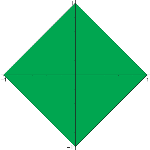
Figure 3: Newtons polygons of curves in Figure 5

The number of tentacles in a given direction is the number of points of $P$ on the corresponding boundary divisor.

2.3 Logarithmic Gauß map

Since $(\mathbb{C}^{\times})^{2}$ is an abelian group, the tangent spaces at all points of $(\mathbb{C}^{\times})^{2}$ are canonically identified with tangent space $T_{(1,1)}$ at the identity $(1,1)\in(\mathbb{C}^{\times})^{2}$. Mapping the tangents to $P$ to their images in $\mathbb{P}(T_{(1,1)})$ gives the logarithmic Gauß map

$$\gamma_{P}:\widetilde{P}\to\mathbb{P}^{1}\,,$$

where $\widetilde{P}$ is the normalization of $P$. In coordinates,

$$\gamma_{P}((z,w))=\frac{z\frac{\partial}{\partial z}P}{w\frac{\partial}{\partial w}P}\,.$$

Note that the values of $\gamma_{P}$ at the boundary points of $P$ are determined by the slopes of the corresponding edges of $\Delta_{P}$.

The degree of $\gamma_{P}$ can be computed as follows, cf. [11, 20]. Recall that the multiplicity $m(p)$ of a point $p\in P$ is the multiplicity with which $P$ intersects a generic line through $p$. Another important characteristic of a singular point is its Milnor number $\mu(p)$, see [22]. It may be defined as the local intersection number of $\frac{\partial}{\partial z}P=0$ and $\frac{\partial}{\partial w}P=0$ at $p$.

Proposition 2.1.

We have

$$\deg\gamma_{P}=2|\Delta^{\circ}_{P}|+|\partial P|-2-\sum_{p\in P}(\mu(p)+m(p)-1)\,.$$ (8)

where $|\Delta^{\circ}_{P}|$ is the number of points in the interior of the Newton polygon $\Delta_{P}$ and $|\partial P|$ is the number of boundary points of $P$ not counting multiplicity.

Clearly, only singular points of $P$ contribute to the sum over $p\in P$ in (8) since for a nonsingular point $p$ we have $m(p)=1$ and $\mu(p)=0$.

Proof.

If $P$ is smooth and transverse to the boundary then the proposition follows from Kouchnirenko’s formula [18] (also using Pick’s formula for the area of a lattice polygon).

A singular point of $P$ subtracts $\mu(p)+m(p)-1$, which is the same computation as for the ordinary Gauß map, see e.g. Theorem 7.2.2. in [28]. The effect of tangency to the boundary is determined similarly, see e.g. Section 4.2 below. ∎

The critical points of $\gamma_{P}$ are known as the logarithmic inflection points. Note that, for example, a cusp is not a logarithmic inflection point, but a sharp, or ramphoid, cusp (locally looking like $x^{2}=y^{5}$) is. By the Riemann-Hurwitz formula applied to $\gamma_{P}$, the count of logarithmic inflection points with multiplicity is

$$\textup{\# logarithmic inflection points}=2\deg\gamma_{P}-\chi(\widetilde{P}).$$ (9)

2.4 Geometric genus and adjunction

The geometric genus of $P$ is defined as the genus $g(\widetilde{P})$ of its normalization $\widetilde{P}$. It may be computed as follows, cf. [15],

$$g(\widetilde{P})=|\Delta^{\circ}_{P}|-\frac{1}{2}\sum_{p\in P}(\mu(p)+\beta(p)-1)$$ (10)

where $\beta(p)$ is the number of branches of $P$ through $p$. This is known as the adjunction formula.

The number $\frac{1}{2}(\mu(p)+\beta(p)-1)$ is a nonnegative integer which vanishes if $p$ is a smooth point of $P$. It equals $1$ for cusps and nodes, so if the curve has only those singularities, we get

$$\textup{\# cusps}+\textup{\# nodes}=|\Delta^{\circ}_{P}|-g(\widetilde{P})\,.$$ (11)

Combining (8) and (10) we get

$$\sum_{p\in P}(m(p)-\beta(p))=-\deg\gamma_{P}-\chi(\widetilde{P}\smallsetminus\partial P)\,.$$ (12)

Remark 2.2.

A geometrically-minded reader might appreciate the following alternative proof (or rather a rephrasing of the proof) of 12.

Suppose that $\widetilde{P}\smallsetminus\partial P$ is smooth. We may deduce the equation

$$\deg\gamma_{P}=-\chi(\widetilde{P}\smallsetminus\partial P)$$ (13)

by the following application of the maximum principle, cf. [19]. Let $\lambda:\mathbb{R}^{2}\to\mathbb{R}$ be a linear map which we may choose with a generic slope of the kernel. The function $\lambda\circ\operatorname{Log}$ is a pluriharmonic function on $(\mathbb{C}^{\times})^{2}$ and thus restricts to a harmonic function $h$ on $\deg\gamma_{P}=-\chi(\widetilde{P}\smallsetminus\partial P)$. Thus all critical points of $h$ are of index 1.

Furthermore, $h$ exhibits $P$ as a cobordism between $P_{-}\subset\partial P$ and $P_{+}\subset\partial P$, where the splitting $\partial P=P_{+}\cup P_{-}$ corresponds to $h^{-1}(+\infty)$ and $h^{-1}(-\infty)$. Thus, the number of critical points of $h$ equals $\chi(P-P_{+},P_{-})=\chi(P\smallsetminus\partial P)$ (the latter equality follows from additivity of Euler characteristic). On the other hand the number equals $\deg\gamma_{P}$, so we get (13). Each singularity $p$ of $P_{-}\subset\partial P$ subtracts $\sum(\mu(P)-\beta(p)-1)$ from $-\chi(P)$ and $\sum(\mu(P)-m(p)-1)$ from $\deg\gamma_{P}$.

2.5 Nodal and cuspidal numbers of a plane curve

The right-hand side of (12) may be interpreted as the total cuspidal number $c(P)$ of $P$. It equals the number of cusps if $P$ has only cusps and ordinary multiple points. An example of formula (12) may be seen in Figure 4. In the bottom half of Figure 4, we see two inflection point come together to form a point of the form $y=x^{4}$. For the dual curves, which have the same genus and the same degree of the logarithmic Gauß map, we see a merger of cusps into a $E_{6}$ singularity $y^{3}=x^{4}$ which has the cuspidal number equal to 2.

Figure 4: Two cusps coalescing in a $E_{6}$ singularity.

Another useful number is the nodal number $b(P)$. First we define the local nodal number $b_{s}(P)$ at every singular point $s\in P$ as the sum $\sum\limits_{j\neq k}\#(B_{j},B_{k})$ of the intersection numbers over all distinct pairs of branches $B_{j}$, $B_{k}$ via $s$. Clearly, $b_{s}(P)=0$ if and only if $s$ is a locally irreducible singular point of $P$. If $s$ is an ordinary node of $P$ then $b_{s}(P)=1$. The nodal number $b(P)$ is the sum of the local nodal numbers over all singular points of $P$.

In many applications the numbers $c(P)$ and $b(P)$ play the rôle of the total numbers of cusps and nodes even if $P$ has higher singularities.

2.6 Integration w.r.t. Euler characteristic

Because of the equation

$$\chi(A\cap B)=\chi(A)+\chi(B)-\chi(A\cap B)$$

the Euler characteristic may be viewed as a signed finite-additive measure. If $f$ is a function on $X$ taking finite many values, its integral with respect to the Euler characteristic is defined by

$$\int_{X}f\,d\chi=\sum_{y}y\,\chi(f^{-1}(y))\,.$$

Calculus of such integrals was developed by O. Viro [27]. Applications of this calculus to the classical Plücker and Klein formulas may also be found in [27].

More generally, given a map

$$F:X\to Y$$

one may push-forward $F_{*}f$ of $f$ by the formula

$$\left[F_{*}f\right](y)=\int_{F^{-1}(y)}f\,d\chi\,.$$

Under additional hypotheses on $F$ and $f$, this operation has natural functorial properties like $(FG)_{*}=F_{*}G_{*}$, see e.g. Section 7.3 in [28]. The case of main importance for us will be when $F$ is a nonconstant map of smooth curves, in which case,

$$F_{*}1=\deg F-\operatorname{br}F\,,$$

where $\operatorname{br}F$ is the branch divisor of $F$, that is, the sum of all critical points of $F$ with their multiplicities.

3 The equation of $R$

3.1 $R$ as a Resultant

Consider the curve $\mathcal{R}$ defined by the equations

$$P(az,bw)=Q(z,w)=\det\begin{pmatrix}\frac{\partial}{\partial z}P(az,bw)&\frac{\partial}{\partial z}Q\vspace{2 mm}\\ \frac{\partial}{\partial w}P(az,bw)&\frac{\partial}{\partial w}Q\end{pmatrix}=0\,.$$ (14)

in $(\mathbb{C}^{\times})^{2}\times(\mathbb{C}^{\times})^{2}$. We have $\mathcal{R}\subset\mathcal{S}$, where the surface $\mathcal{S}$ was defined in (3). In general, $\mathcal{R}$ may have several components. The Wronskian in (14) vanishes at any singular point of $q$ of $Q$, hence such a point contributes a translate of $P$ to $\mathcal{R}$. The multiplicity of this component equals $m(q)+\mu(q)-1$, see the proof of Proposition 2.1. Symmetrically, singular points of $P$ contribute copies of $Q$ to $\mathcal{R}$. The remaining components correspond to actual tangency. The curve $R$ is the projection of these components to the $(a,b)$-plane.

The equation of $R$ may be found by eliminating $z$ and $w$ from (14), followed by factoring off spurious components caused by singularities. Gröbner basis algorithms give one way to perform this elimination. We find that in practice it is easier and faster to use resultants for this computation.

Consider the polynomial

$$R_{1}(a,b,z)=\textup{resultant}_{w}\big{(}P(az,bw),Q(z,w)\big{)}\,.$$

The equation $R_{1}(a,b,z)=0$ cuts out the image $\mathcal{S}_{1}$ of $\mathcal{S}$ under the projection along the $z$ direction. This projection may create singularities, specifically $\mathcal{S}_{1}$ may intersect itself along curves. Consider

$$R_{2}(a,b)=\textup{resultant}_{z}\left(R_{1},\frac{\partial}{\partial z}R_{1}\right)\,.$$

Its zero locus consists of critical points of the projection of $\mathcal{S}_{1}$ along the $z$ direction, together with contributions of singularities. Those can be identified and removed by factoring $R_{2}$ as they all occur with multiplicity greater than one. For example, the image of double point curves of $\mathcal{S}_{1}$ will occur in $R_{2}$ with multiplicity two.

Exact factorization is possible and rather effective for polynomials with rational coefficients. In probabilistic applications, the coefficients may be known only approximately, making exact factorization impossible. This is why it is useful to know the Newton polygon of $R$, which will be determined below. Also note that sometimes, albeit rarely, components of $R$ may occur with multiplicity in $R_{2}$ as, for example, in (4).

3.2 Multiplicity of tangency

Given two curves $C$ and $C^{\prime}$ and a point $p$ define their tangency multiplicity at $p$ as

$$(C\curlywedge C^{\prime})_{p}=(C\cdot C^{\prime})_{p}-m_{C}(p)\,m_{C^{\prime}}(p)$$

where $(C\cdot C^{\prime})_{p}$ is the local intersection multiplicity of $C$ and $C^{\prime}$ at $p$ and $m_{C}(p)$ is the multiplicity of the point $p$ on $C$. Note that $(C\curlywedge C^{\prime})_{p}=0$ if $p\notin C$ or if $C$ and $C^{\prime}$ intersect transversely at $p$. Also note that the tangency multiplicity is additive over branches of both $C$ and $C^{\prime}$.

We have the following

Proposition 3.1.

The multiplicity of a point $(a,b)\in R$ is the total tangency multiplicity of $P(az,bw)=0$ and $Q(z,w)=0$, assuming they are not tangent at infinity.

In other words, the local cuspidal number at each branch of a singular point of $R$ is equal to the corresponding tangency multiplicity minus one.

Proof.

Since multiplicity is a local quantity, we can work with the additive version (6). We may work with each branch of the singularity individually. Suppose $P$ and $Q$ are tangent at $z=w=0$ and that $w=0$ is their common tangent. In this case the origin will belong to $P-Q$ and $b=0$ will be the corresponding tangent. We need to compute the total multiplicity $m_{R}$ of all branches of $R$ corresponding to this tangency. It equals the number of roots $b_{i}$ of $R(\epsilon,b)=0$ with $b_{i}\approx 0$ where $\epsilon$ is a fixed small nonzero number. For $b=b_{i}$ the curves

$$P(z+\epsilon,w+b)=0\,,\quad Q(z,w)=0\,,$$ (15)

are tangent.

Consider the intersection $U$ of the curve defined by (15) in the $(z,w,b)$-space with a neighborhood of the origin. We will compute the Euler characteristic of $U$ in two different ways. Viewing $U$ as a degree $m_{P}\,m_{Q}$ branched covering of the $z$ line, we get

$$\chi(U)=-m_{P}\,m_{Q}+m_{P}+m_{Q}\,,$$

where $m_{P}$ and $m_{Q}$ is the multiplicity of the origin on $P$ and $Q$, respectively.

On the other hand, we may view $U$ as a branched covering of the $b$-line. It has degree $(P\cdot Q)_{0}$, where $(P\cdot Q)_{0}$ is the intersection multiplicity of $P$ and $Q$ at the origin. We have

$$\chi(U)=(P\cdot Q)_{0}-m_{P}(m_{Q}-1)-m_{Q}(m_{P}-1)-m_{R}$$

because each tangency in (15) corresponds to a simple branchpoint. This concludes proof. ∎

4 Newton polygon of log-front

4.1 Formula for $\Delta_{R}$

Let $\Delta_{P}$ and $\Delta_{Q}$ denote the marked Newton polytopes of $P$ and $Q$. We denote by $-\Delta_{Q}$ the reflection of $\Delta_{Q}$ about the origin, with the corresponding marking.

We say that two edges $E$ and $F$ are opposite and write $E\rightleftarrows F$, if their outward normals point in the opposite direction. As we will see, in the simplest case when no edge of $-\Delta_{Q}$ is opposite to an edge of $\Delta_{P}$, the Newton polygon $\Delta_{R}$ is simply the Minkowski sum

$$\deg(\gamma_{Q})\cdot\Delta_{P}+\deg(\gamma_{P})\cdot(-\Delta_{Q})\,.$$ (16)

Every pair of opposite edges $E\subset\Delta_{P}$ and $F\subset-\Delta_{Q}$ makes the polygon $\Delta_{R}$ smaller than (16).

Given two partitions $\lambda$ and $\mu$, we define

$$\langle\lambda,\mu\rangle =\sum_{i}\lambda^{\prime}_{i}\,\mu^{\prime}_{i}$$ (17)

$$=\sum_{i,j}\min(\lambda_{i},\mu_{j})\,,$$ (18)

where $\lambda^{\prime}$ denotes the conjugate partition. The equivalence of (17) and (18) is an elementary combinatorial fact.

Given an edge $E$, let

$$\mathbf{n}_{E}=\frac{E}{|E|}$$

is the unit (non-oriented) lattice segment in the direction of $E$. Note that (similarly to Newton polygons) such lattice segments are defined only up to translations by $\mathbb{Z}^{2}$.

Theorem 1.

The Newton polygon of the log-front $R$ is the unique polygon $\Delta_{R}$ satisfying

$$\Delta_{R}+\sum_{E\rightleftarrows F}\langle\lambda(E),\lambda(F)\rangle\,\mathbf{n}_{E}=\deg(\gamma_{Q})\cdot\Delta_{P}+\deg(\gamma_{P})\cdot(-\Delta_{Q})\,,$$ (19)

where the summation is over all pairs $E\subset\Delta_{P}$ and $F\subset-\Delta_{Q}$ of opposite edges and $\lambda(E)$ are the corresponding partition markings, i.e. multiplicities of intersection with the boundary.

Minkowski “subtraction” of segments, implicit in formula (19), simply reduces the length of all edges in that direction by the given amount.

4.2 Proof

By definition, a boundary point of $R$ is a tangency of the curves $P$ and $Q$, dilated with respect to one another by an infinite amount. In logarithmic coordinates, infinite dilation becomes an infinite shift. Shifted by an infinite amount, the amoeba $\operatorname{Log}(P)$ of $P$ is either a union of parallel lines (tentacles) or empty, in which case there will not be any boundary points of $R$ in this direction. This is illustrated in Figure 5.

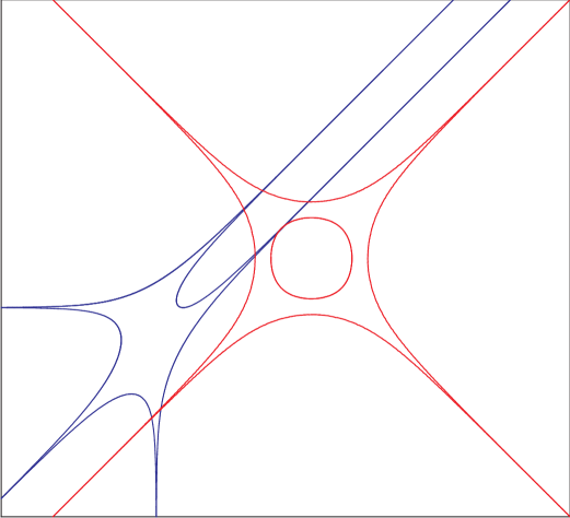
Figure 5: Tangency to a tentacle creates a boundary point of a log-front

Tangency to a tentacle occurs at points mapped by the logarithmic Gauß map to the slope of the tentacle. Therefore, if $\operatorname{Log}(P)$ and $\operatorname{Log}(Q)$ do not have tentacles in the same direction (that is, $\Delta_{P}$ and $\Delta_{Q}$ have no parallel edges) then each tentacle of $\operatorname{Log}(P)$ contributes $\deg\gamma_{Q}$ points to $\partial R$. The multiplicity of the resulting point in $\partial R$ equals the multiplicity of the corresponding point of $\partial P$.

The effect of a tentacle-to-tentacle tangency may be studied in a local model, for example,

$$P=\{w-(z-1)^{k}\}\,,\quad Q=\{w-(z-1)^{l}\}\,.$$

In this case,

$$\gamma_{P}(z)\sim\frac{k}{z-1}\,,\quad\gamma_{Q}(z)\sim\frac{l}{z-1}\,,\quad z\to 1\,,$$

Equating $\gamma_{P}(az)=\gamma_{Q}(z)$ gives a parametrization of $R$ such that

$$a\sim 1,\quad b\propto(z-1)^{k-l}\,,\quad z\to 1\,.$$ (20)

This means that tentacles of $P$ and $Q$ pointing in the opposite direction (which means that $k$ and $l$ have opposite sign) produce a tentacle of combined multiplicity $|k|+|l|$ pointing in the same direction as the $P$-tentacle. Tentacles pointing in the same direction, by contrast, produce a tentacle of multiplicity $|k-l|$ pointing in one of the two directions. This rule can be phrased more naturally in terms of the reflected Newton polygon $-\Delta_{Q}$ because the reflection flips the direction of tentacles.

The polygons $\Delta_{P}$ and $-\Delta_{Q}$ can, in total, have as many as 4 edges with the same slope. Let $E,\overline{E}\subset\Delta_{P}$ and $F,\overline{F}\subset-\Delta_{Q}$ be such a 4-tuple of edges and let $\lambda(E),\dots$ denote the partition marking. Assume that the outward normals to $E,F$ point in the same direction. By our computations, the polygon $\Delta_{R}$ will have an edge in the same direction as $E$ and $F$ of length

$$|E|(\deg\gamma_{Q}-\ell(\lambda(F))-\ell(\lambda(\overline{F})))+|F|(\deg\gamma_{P}-\ell(\lambda(E))-\ell(\lambda(\overline{E})))$$

$$+\sum_{i,j}\left(\lambda(E)_{i}+\lambda(F)_{j}\right)+$$ (21)

$$\sum_{i,j}\max(\lambda(E)_{i}-\lambda(\overline{F})_{j},0)+\sum_{i,j}\max(\lambda(F)_{i}-\lambda(\overline{E})_{j},0)\,.$$

Note that the middle line in (21) cancels with a part of the first line. A further cancellation is obtained from

$$-|E|\,\ell(\lambda(\overline{F}))+\sum_{i,j}\max(\lambda(E)_{i}-\lambda(\overline{F})_{j},0)=-\sum_{i,j}\min(\lambda(E)_{i},\lambda(\overline{F})_{j})$$

using formula (18). This concludes proof.

Counting the boundary points of $R$ without respect to the corresponding direction $\mathbf{n}_{E}$ gives us the following corollary.

Corollary 4.1.

The cardinality of $|\partial R|$ equals to

$$\deg\gamma_{P}|\partial\Delta_{Q}|+\gamma_{Q}|\partial\Delta_{P}|-\sum_{E\rightleftarrows F}\langle\lambda(E),\lambda(F)\rangle.$$

4.3 Examples

Let $P$ and $Q$ be generic with Newton polygons from Figure 3. In this case, the Newton polygon $\Delta_{R}$ is the larger of the two polygons plotted in Figure 6. If $P$ develops a tangency to the boundary then $\Delta_{R}$ shrinks and becomes the smaller polygon in Figure 6. What happens in this case, is that $R$ becomes reducible with one component being a boundary divisor. The boundary divisor corresponds to tangency with $P$ at the newly developed point of tangency to infinity.

Figure 6: Possible $\Delta_{R}$ for $\Delta_{P}$ and $\Delta_{Q}$ from Figure 3.

As another example, consider the case when $P$ and $Q$ are generic curves of degree $d_{P}$ and $d_{Q}$. In this case, both $\Delta_{P}$ and $\Delta_{Q}$ are triangles with sides of length $d_{P}$ and $d_{Q}$, while $\Delta_{R}$ is a hexagon with sides of length

$$d_{P}d_{Q}(d_{Q}-1),d_{Q}d_{P}(d_{P}-1),\dots\,,$$

cyclically repeated. In particular, when $d_{P}=1$ we get a triangle with side $d_{Q}(d_{Q}-1)$, reproducing the very classical formula for the degree of dual curve.

In the example in Figure 2, the degrees of logarithmic Gauss maps of $P$ and $Q$ are $4$ and $10$ respectively, hence $\Delta_{R}$ is a hexagon with sides $8$ and $12$.

4.4 Reconstructing the curve $Q$ by the log-front $R$

It is instructive to have a closer look at the computation done in (20) in the case $k=l$. In this case, the point $(a,b)$ does not escape at infinity, but it is still a pole of the logarithmic Gauss map of $R$ (see also Section 5.1 below). In other words, the curve $R$ is tangent to $a=1$ at the corresponding point.

In probabilistic applications, the curve $P$ is given and one knows that the frozen boundary is compact and tangent to given lines. This allows to fix the real boundary points of $Q$ and their multiplicities (which have to match the corresponding multiplicities for $P$). In particular, this is how the curve $Q$ in Figure 1 is determined from the requirement that the frozen boundary in Figure 2 is inscribed in a hexagon.

5 Plücker-type formulas for $R$

5.1 Logarithmic Gauß map of $R$

Let $\widehat{R}$ be the product of the normalizations $\widetilde{P}$ and $\widetilde{Q}$ over their logarithmic Gauß maps:

(22)

In English, a point of $\widehat{R}$ corresponds to a tangency of a branch of $P$ to a translate of a branch of $Q$. Note that $\widehat{R}$ is a partial normalization of the plane curve $R$: we have the factorization $\widetilde{R}\to\widehat{R}\to R$ for the normalization $\widetilde{R}\to R$. We claim that the logarithmic Gauß map of $\widetilde{R}$ factors through the natural map $\widetilde{R}\to\widehat{R}$.

Proposition 5.1.

The logarithmic Gauß map for $R$ is the composition

$$\widetilde{R}\to\widehat{R}\overset{\gamma_{R}}{\to}\mathbb{P}^{1}$$

Proof.

The essential geometric content of this result is already implicit in (4). In coordinates, the claim is elementary to check on the open dense set where tangency is nondegenerate. It suffices to analyze the Gauss map of the additive analog $P-Q$ of the log front $P\div Q$. Let $P$ and $Q$ be given by

$$y=P(x)\,,\quad y=Q(x)\,.$$

Then $P-Q$ is parametrized by

$$(x-s,P(x)-Q(s))$$

where $s=s(x)$ is a solution of $P^{\prime}(x)=Q^{\prime}(s)$. The Gauss map of the above curve is clearly $P^{\prime}(x)=Q^{\prime}(s)$. ∎

Corollary 1.

$$\deg\gamma_{R}=\deg\gamma_{P}\,\deg\gamma_{Q}\,.$$ (23)

5.2 Geometric genus of $R$

The geometric genus of $R$, or equivalently, the Euler characteristic $\chi(\widetilde{R})$ can be computed by Riemann-Hurwitz formula applied to the map $\gamma_{R}$ in (22). To do this we need to be able to compare $\chi(\widetilde{R})$ and $\chi(\widehat{R})$.

The map $\gamma_{R}$ is ramified over the branchpoints of either $\gamma_{P}$ or $\gamma_{Q}$. Suppose that at a point $p\in\widetilde{P}$ the map $\gamma_{P}$ is given by

$$x\to x^{\nu}\,,\quad\nu=1,2,\dots\,,$$ (24)

in a suitable local coordinate $x\in\mathbb{C}$ centered at $p$. In other words, suppose that $p$ is a logarithmic inflection point of multiplicity $\nu-1$. Note that such point may be singular or non-singular point of $P$. This integer $\nu$ will be denoted by $\nu(p)$.

A point of $\widehat{R}$ is a pair $(p,q)\in\widetilde{P}\times\widetilde{Q}$ such that

$$\gamma_{P}(p)=\gamma_{Q}(q)=x\in\mathbb{P}^{1}\,.$$

Let $x_{p}$ and $x_{q}$ be local coordinates at $p$ and $q$ as in (24). The local equation of $\widehat{R}$ is

$$x_{p}^{\nu(p)}=x_{q}^{\nu(q)}\,,\quad(x_{p},x_{q})\in\mathbb{C}^{2}\,.$$

This has $\gcd(\nu(p),\nu(q))$ branches and hence produces $\gcd(\nu(p),\nu(q))$ points

$$r_{1},\dots,r_{\gcd(\nu(p),\nu(q))}\in\widetilde{R}$$

that are mapped to $x$ by the logarithmic Gauß map. Each is a logarithmic inflection point of multiplicity $\operatorname{lcm}(\nu(p),\nu(q))-1$. Note that while all $r_{i}\in\widetilde{R}$ are logarithmic inflection points of the same multiplicity, the multiplicities of the corresponding branches of $R$ may be different and are not determined by the numbers $\nu(p)$ and $\nu(q)$.

From definitions

$$\chi(\widehat{R})=\int_{\widehat{R}}1\,d\chi=\int_{\mathbb{P}^{1}}(\gamma_{P})_{*}1\,(\gamma_{Q})_{*}1\,d\chi\,.$$ (25)

We conclude

Theorem 2.

The Euler characteristic $\chi(\widetilde{R})$ is given by

$$\chi(\widetilde{R})=\chi(\widehat{R})+\sum_{\gamma_{P}(p)=\gamma_{Q}(q)}(\gcd(\nu(p),\nu(q))-1)$$

where $\chi(\widehat{R})=((\gamma_{P})_{*}1,(\gamma_{Q})_{*}1)_{\chi}=-2\deg\gamma_{P}\,\deg\gamma_{Q}+\chi(\widetilde{P})\,\deg\gamma_{Q}+\chi(\widetilde{Q})\,\deg\gamma_{P}$.

The above inner product with respect to the Euler characteristic is defined as in (25). Note that generically the the branchpoints of $\gamma_{P}$ are disjoint from branchpoints of $\gamma_{Q}$. In this case, the above formulas may be simplified as follows.

Corollary 2.

If tangency does not occur at two logarithmic inflection points then

$$\chi(\widetilde{R})=\chi(\widehat{R})=-2\deg\gamma_{P}\,\deg\gamma_{Q}+\chi(\widetilde{P})\,\deg\gamma_{Q}+\chi(\widetilde{Q})\,\deg\gamma_{P}\,.$$ (26)

5.3 Nodes and cusps of $R$

The total cuspidal number of $R$ may now be determined using the formula (12).

Theorem 3.

We have the following expressions for the cuspidal number $c_{{R}}$ of the resultant curve $R=R(P,Q)$.

$$c(R)=-\chi(\widetilde{R})+|\partial R|-(\chi(\widetilde{P})+c(P)-|\partial P|)(\chi(\widetilde{Q})+c(Q)-|\partial Q|).$$

Proof.

This formula can be obtained as a straightforward combination of (12) and Corollary 1. Nevertheless it is instructive to prove it by the Viro calculus (see Section 2.6) to prepare a way for the real counterpart in the next section.

Consider the family of translates $\tau_{s}({P})$ parameterized by $s\in(\mathbb{C}^{\times})^{2}$. Denote with $X(s)$ the Euler characteristic of the space of pairs $(t_{P},t_{Q})\in\tilde{P}\times\tilde{Q}$, such that $\tau_{s}(t_{P})=t_{Q}$. We have

$$\int\limits_{(\mathbb{C}^{\times})^{2}}X(s)d\chi(s)=(\chi(\tilde{P})-|\partial P|)(\chi(\tilde{Q})-|\partial Q|).$$ (27)

It may be viewed as a corollary of the Fubini theorem since each pair of points from $\tilde{P}\smallsetminus\partial P$ and $\tilde{Q}\smallsetminus\partial Q$ will appear in $X(s)$ once. On the other hand we have

$$\int\limits_{(\mathbb{C}^{\times})^{2}}X(s)d\chi(s)=-\chi(\tilde{R})+|\partial R|\\ -c(P)(\chi(\tilde{Q})-|\partial Q|)-c(Q)(\chi(\tilde{P})-|\partial P|)-c(P)c(Q)-c(R).$$ (28)

Indeed, we have $\chi((\mathbb{C}^{\times})^{2})=0$ while $X(s)$ is constant for generic $s\in\mathcal{T}$ (namely, by Bernstein-Kouchnirenko formula it is equal to $\operatorname{Vol}(\Delta_{P},\Delta_{Q})$). However the value $X(s)$ drops if $s\in R$ and it drops further (by $m-1$) if there is a singular point of multiplicity $m$ at a branch of $\tilde{R}\smallsetminus\partial R$ through $s$ or if $\tau_{s}(\widetilde{P})$ and $\widetilde{Q}$ have a tangency of higher order (which in turn corresponds to a cusp of $\tilde{R}$). We get the theorem as the combination of (27) and (28). ∎

If $P$ and $Q$ are generic, the only singularities of $R$ will be cusps and nodes and the nodal number of $R$ may be recovered from the adjunction formula.

For example, let $P$ and $Q$ be generic curves of degree $d_{P}$ and $d_{Q}$. In this case

$$\chi(\widetilde{R})=-d_{P}d_{Q}(4d_{P}d_{Q}-3d_{P}-3d_{Q})\,.$$

Note that this grows very fast with $d_{P}$ and $d_{Q}$. Already when $P$ and $Q$ are generic conics, the geometric genus of $R$ is $9$.

The Newton polygon of $R$ and its boundary were determined above in Section 4.3. Generically, $R$ will not have multiple point on the boundary. For the number of cusps Theorem 3 produces

$$\textup{\# cusps}=3d_{P}^{2}d_{Q}^{2}-6d_{P}d_{Q}\,.$$

Accordingly for the number of nodes we get:

$$\textup{\# nodes}=\frac{d_{P}^{4}d_{Q}^{2}}{2}+2d_{P}^{3}d_{Q}^{3}+\frac{d_{P}^{2}d_{Q}^{4}}{2}-3d_{P}^{3}d_{Q}^{2}-3d_{P}^{2}d_{Q}^{3}-2d_{P}^{2}d_{Q}^{2}+9d_{P}d_{Q}\,.$$

For $d_{P}=1$, these specialize to the classical Plücker formulas. The last two formulas were obtained in [7].

6 Klein-type formula for the log-front $R$

6.1 Refinement of the nodal and cuspidal numbers

For this section it will be important that both $P$ and $Q$ are defined over the field $\mathbb{R}$ of real numbers. In this case, clearly, the curve $R$ is defined over $\mathbb{R}$ as well.

An algebraic curve $P\subset\mathcal{T}$ is defined over $\mathbb{R}$ if and only if it is invariant with respect to the involution of complex conjugation $\operatorname{conj}:\mathcal{T}\to\mathcal{T}$. The fixed point locus of this involution is the real toric surface $\mathbb{R}\mathcal{T}\subset\mathcal{T}$. The real locus $\mathbb{R}{P}$ coincides with the intersection $P\cap\mathbb{R}\mathcal{T}$.

For a real curve $P$ we may refine both the cuspidal number $c(P)$ and the nodal number $b(P)$ as follows. Let $c^{\operatorname{Re}}(P)$ be the number of cusps of $P$ (counted with multiplicity as in Section 2.5) that are real, i.e. contained in $\mathbb{R}T_{\Delta}$. In other words, to get $c^{\operatorname{Re}}(P)$ we add over (real and imaginary) branches of real singular points of $P$ the multiplicities of these branches diminished by 1. We set $c^{\operatorname{Im}}(P)=c(P)-c^{\operatorname{Re}}(P).$

Let $b^{\operatorname{Re}}_{+}(P)$ be the sum over all singular points $s$ of $P$ in $\mathbb{R}\mathcal{T}$ of the number of the pairs of conjugate imaginary branches of $P$. If $s\in\mathbb{R}P$ is a singular point we may introduce $b^{\operatorname{Re}}_{-}(P,s)$ as the sum of the local intersection numbers over all possible pairs of the real branches of $P$ at $s$. Let $b^{\operatorname{Re}}_{-}(P)$ be the sum of $b^{\operatorname{Re}}_{-}(P,s)$ over all real singular points of $P$ and let $b^{\operatorname{Im}}(P)=b(P)-b^{\operatorname{Re}}_{+}(P)-b^{\operatorname{Re}}_{-}(P)$.

Thus we get the refinements

$$c(P)=c^{\operatorname{Re}}(P)+c^{\operatorname{Im}}(P)$$

and

$$b(P)=b^{\operatorname{Re}}_{+}(P)+b^{\operatorname{Re}}_{-}(P)+b^{\operatorname{Im}}(P).$$

In the case when the only singularities of $P$ are ordinary cusps and nodes the numbers $c^{\operatorname{Re}}(P)$ and $c^{\operatorname{Im}}(P)$ are the numbers of real and complex cusps respectively while the numbers $b^{\operatorname{Re}}_{-}(P),b^{\operatorname{Re}}_{+}(P)$ and $b^{\operatorname{Im}}(P)$ are the numbers of real hyperbolic ($A_{1}^{-}$), real elliptic ($A_{1}^{+}$) and imaginary nodes.

It is convenient to define the boundary nodal number $b(\partial P)$ to be equal to the sum of the multiplicities of the boundary points of $P$ minus the simple cardinality of $\partial P$. (Note that since $\partial P$ is 0-dimensional this boundary nodal number also works as the boundary counterpart of the cuspidal number.) Again we have the refinement $b(\partial P)=b^{\operatorname{Re}}(\partial P)+b^{\operatorname{Im}}(\partial P)$ that counts real and imaginary boundary points separately. Thus $b^{\operatorname{Re}}(\partial P)$ is the measure of nontransversality of the real locus $\mathbb{R}P$ to the boundary divisor of the toric surface $\mathcal{T}$.

6.2 Computations for $R$

In general, the set of refined nodal and cuspidal numbers $b^{\operatorname{Re}}_{+},b^{\operatorname{Re}}_{-},c^{\operatorname{Re}},c^{\operatorname{Im}}$ for the log-front $R$ is not determined by the corresponding sets for $P$ and ${Q}$. Let us recall a well-known example illustrating this in the case of classical projective duality, i.e. if $P$ is given by the polynomial $z+w+1$: two real inflection points may disappear together with a bitangent real line.

Example 6.1.

Let $\mathbb{R}Q_{1},\mathbb{R}Q_{2}\subset{\mathbb{R}}{\mathbb{P}}^{2}$ be real quartic curves pictured in Figure 7. The first curve can be constructed by perturbation of the union of two ellipses while the second one can be constructed by perturbation of the union of four lines. We have $b^{\operatorname{Re}}_{+}({R_{1}})=0,c^{\operatorname{Re}}({R_{1}})=8,b^{\operatorname{Re}}_{+}({R_{2}})=4,c^{\operatorname{Re}}({R_{1}})=0$.

Figure 7: Real quartic curves $\mathbb{R}Q_{1}$ and $\mathbb{R}Q_{2}$ whose projective duals have distinct $b^{\operatorname{Re}}_{+}$ and $c^{\operatorname{Re}}$.

The classical Klein’s formula [16] allows us to compute $2b^{\operatorname{Re}}_{+}(\bar{R})+c^{\operatorname{Re}}(\bar{R})$ in the case when $P$ is a line. To generalize this statement for a larger class of real curves $P$ let us look at the argument map $\operatorname{Arg}:(\mathbb{C}^{\times})^{2}\to S^{1}\times S^{1}$ defined by

$$\operatorname{Arg}(z,w)=(\arg(z),\arg(w)).$$

The image $\operatorname{Arg}(A)\subset S^{1}\times S^{1}$ is called the coamoeba or the alga of $A\subset(\mathbb{C}^{\times})^{2}$, cf. [23], [8].

The real 2-torus $S^{1}\times S^{1}$ is a group which has $\mathbb{Z}_{2}\times\mathbb{Z}_{2}$ as its subgroup. Let $T=S^{1}\times S^{1}/\mathbb{Z}_{2}\times\mathbb{Z}_{2}$ be the quotient group and $\beta:S^{1}\times S^{1}\to T=S^{1}\times S^{1}/\mathbb{Z}_{2}\times\mathbb{Z}_{2}$ be the projection map. Note that $T$ is itself a group isomorphic to $S^{1}\times S^{1}$ and the zero in this group is $0_{T}=\beta(1,1)$.

We need to compactify the map $\beta\circ\operatorname{Arg}:P\smallsetminus\partial P\to T$. Note that this map does not extend to $P$. Let us consider $\hat{P}$ to be the real blow-up of $\tilde{P}$ at the finite collection of points $\partial P\subset\tilde{P}$. Naturally, $\hat{P}$ is a closed non-orientable surface whose Euler characteristic coincides with that of $\tilde{P}\smallsetminus{\partial P}$ (in the case of non-compact spaces we use Euler characteristic for homology with closed support) Furthermore, we have a natural extension

$$\operatorname{Alga}_{P}:\hat{P}\to T$$

such that $\operatorname{Alga}_{P}|_{\tilde{P}\smallsetminus\partial P}=\beta\circ\operatorname{Arg}|_{\tilde{P}\smallsetminus\partial P}$.

Consider the following integral

$$I_{\mathbb{R}}=\int\limits_{t\in\mathbb{R}\mathcal{T}\smallsetminus\operatorname{Vert}(\mathbb{R}\mathcal{T})}X(t)d\chi_{\mathbb{R}\mathcal{T}}(t)$$

(note that here we use the family $\tau_{t}(P)$ only for $t\in\mathbb{R}\mathcal{T}$). This integral is the real counterpart of the integral (27) from the proof of Theorem 3 where we defined the number $X(t)$, but now we use only the real translations.

As in Theorem 3 the integral $I_{\mathbb{R}}$ can be computed in two different ways.

For this computation to depend only on visible characteristics of the curves $P$ and $Q$ we need to assume that $P$ is a Harnack curve (see Appendix A).

Let

$$\epsilon(\Delta_{P},\Delta_{Q})=\sum\limits_{\Delta^{\prime}_{P},\Delta^{\prime}_{Q}}\operatorname{Area}(\Delta^{\prime}_{P}+\Delta^{\prime}_{Q}),$$

where $\Delta^{\prime}_{P}$ (resp. $\Delta^{\prime}_{Q}$) run over all possible sides of the polygon $\Delta_{P}$ (resp. $\Delta_{Q}$) and $\Delta^{\prime}_{P}+\Delta^{\prime}_{Q}$ stands for the parallelogram obtained as the Minkowski sum of the intervals $\Delta^{\prime}_{P}$ and $\Delta^{\prime}_{Q}$.

Proposition 6.2.

If $P$ is a Harnack curve and $Q$ is any curve defined over $\mathbb{R}$ then

$$I_{\mathbb{R}}=2\operatorname{Area}(\Delta_{P})(\chi(\tilde{Q})-2b^{\operatorname{Re}}_{+}({Q})-b^{\operatorname{Re}}(\partial Q)-|\partial\Delta_{Q}|)+\\ (2b^{\operatorname{Re}}_{+}({P})+b^{\operatorname{Re}}(\partial P))(2b^{\operatorname{Re}}_{+}({Q})+b^{\operatorname{Re}}(\partial Q))-\epsilon(\Delta_{P},\Delta_{Q}),$$

Proof.

Note that if two points $s_{P}\in\hat{P}$ and $s_{Q}\in\hat{Q}$ are different by a translation by $t\in\mathbb{R}\mathcal{T}$ then $\operatorname{Alga}_{P}(s_{P})=\operatorname{Alga}_{Q}(s_{Q})$. Conversely, if $\operatorname{Alga}_{P}(s_{P})=\operatorname{Alga}_{Q}(s_{Q})$ and either $s_{P}$ or $s_{Q}$ is not in the exceptional divisor of the blowup map then there exists $t\in\mathbb{R}\mathcal{T}\smallsetminus\operatorname{Vert}(\mathbb{R}\mathcal{T})$ such that $\tau_{t}({P})$ and ${Q}$ have $s_{Q}$ as one of their intersection point. The Euler characteristic of the space formed by the pairs $(s_{P},s_{Q})$ with $\operatorname{Alga}_{P}(s_{P})=\operatorname{Alga}_{Q}(s_{Q})$ and such that $s_{P}$ and $s_{Q}$ are from the exceptional divisors of the blowups $\hat{P}\to\tilde{P}$ and $\hat{Q}\to\tilde{Q}$ respectively is $\epsilon(\Delta_{P},\Delta_{Q})$.

We have $\chi((\operatorname{Alga}_{P})^{-1}(\alpha))=2\operatorname{Area}(\Delta_{P})$ for any $\alpha\in T\smallsetminus\{0_{T}\}$ by Lemma A1. Note that $\chi((\operatorname{Alga}_{Q})^{-1}(T\smallsetminus\{0_{T}\}))=\chi(\hat{Q})-2b^{\operatorname{Re}}_{+}({Q})-b^{\operatorname{Re}}(\partial Q)=\chi(\tilde{Q})-|\partial\Delta_{Q}|-2b^{\operatorname{Re}}_{+}({Q})-b^{\operatorname{Re}}(\partial Q)$. The contribution of $\alpha=0_{T}$ to the left-hand side of Proposition 6.2 is $(2b^{\operatorname{Re}}_{+}({P})+b^{\operatorname{Re}}(\partial P))(2b^{\operatorname{Re}}_{+}({Q})+b^{\operatorname{Re}}(\partial Q))$ since $\mathbb{R}\hat{P}$ is a closed 1-manifold and thus $\chi(\mathbb{R}\hat{P})=0$. ∎

Let $n$ be the number of vertices of the polygon $\Delta_{PQ}=\Delta_{Q}-\Delta_{P}$.

Proposition 6.3.

If $P$ is a Harnack curve and $Q$ is any curve defined over $\mathbb{R}$ immersed near the boundary of $\mathbb{R}\mathcal{T}$ then

$$I_{\mathbb{R}}=\operatorname{Vol}(\Delta_{P},\Delta_{Q})(4-2n)\\ -2\operatorname{Area}(\Delta_{P})c^{\operatorname{Im}}({Q})-(2b^{\operatorname{Re}}_{+}(P)+b^{\operatorname{Re}}(\partial P))c^{\operatorname{Re}}(Q)-(2b^{\operatorname{Re}}_{+}({R})+c_{\operatorname{Re}}({R})).$$

Proof.

The Euler characteristic of $\mathbb{R}\mathcal{T}\smallsetminus\operatorname{Vert}(\mathbb{R}\mathcal{T})$ is $4-2n$. For a generic $t$ we have $X(t)=\operatorname{Vol}(\Delta_{P},\Delta_{Q})$ by the Bernstein-Kouchnirenko formula [2], [18]. This number gets decreased if $\tau_{t}({P})$ and ${Q}$ are tangent or if one of their intersection point is singular for a branch of $\tilde{Q}$ (note that ${P}$ is an immersed smooth curve since it is Harnack). The latter case contributes $-2\operatorname{Area}(\Delta_{P})c^{\operatorname{Im}}({Q})-(2b^{\operatorname{Re}}_{+}(P)+b^{\operatorname{Re}}(\partial P))c^{\operatorname{Re}}(Q)$.

If $\tau_{t}({P})$ and ${Q}$ are tangent at a point in a non-real point then we have a bitangency since both ${P}$ and ${Q}$ are invariant with respect to the involution of complex conjugation. This contributes $-2b^{\operatorname{Re}}_{+}({R})$. The tangencies at real points contribute $\chi(\mathbb{R}\tilde{R})=0$ plus $c_{\operatorname{Re}}({R})$ where the tangencies of $\tau_{t}({P})$ and ${Q}$ are of higher order. ∎

6.3 Klein’s formula

Combining Proposition 6.2 and 6.3 we get the following theorem.

Theorem 4.

If $P$ is a simple Harnack curve and $Q$ is any curve defined over $\mathbb{R}$ immersed near the boundary of $\mathbb{R}\mathcal{T}$ then

$$2b^{\operatorname{Re}}_{+}({R})+c^{\operatorname{Re}}({R})=(4-2n)\operatorname{Vol}(\Delta_{P},\Delta_{Q})+\\ 2\operatorname{Area}(\Delta_{P})(|\partial\Delta_{Q}|-\chi(\tilde{Q})+2b^{\operatorname{Re}}_{+}({Q})+b^{\operatorname{Re}}(\partial Q)-c^{\operatorname{Im}}({Q}))\\ -(2b^{\operatorname{Re}}_{+}({P})+b^{\operatorname{Re}}(\partial P))(2b^{\operatorname{Re}}_{+}({Q})+b^{\operatorname{Re}}(\partial Q)+c^{\operatorname{Re}}(Q))+\epsilon(\Delta_{P},\Delta_{Q}).$$

Corollary 6.4.

Let $\mathbb{R}{P},\mathbb{R}{Q}\in{\mathbb{R}}{\mathbb{P}}^{2}$ be two curves of degree $d_{P}$ and $d_{Q}$ (respectively) not passing via $(0:0:1),(0:1:0),(1:0:0)$. Suppose that $P$ is a simple Harnack curve and ${Q}$ is a smooth curve. Then

$$2b^{\operatorname{Re}}_{+}({R})+c^{\operatorname{Re}}({R})=d^{2}_{P}d^{2}_{Q}-2d_{P}d_{Q}.$$

Proof.

We have $n=6$, $\operatorname{Area}(\Delta_{P})=\frac{d_{P}^{2}}{2}$, $\chi(\tilde{Q})=3d_{Q}-d^{2}_{Q}$, $|\partial\Delta_{Q}|=3d_{Q}$ and $\epsilon(\Delta_{P},\Delta_{Q})=6d_{P}d_{Q}$. ∎

Let us deduce the Klein formula [17] in its classical form from Theorem 4 in the case when $P$ is a line $z+w+1=0$ and $\mathbb{R}Q$ is a curve of degree $d$ in ${\mathbb{R}}{\mathbb{P}}^{2}$ not passing via $(0:0:1),(0:1:0),(1:0:0)$. In this case $\Delta_{Q}$ is a triangle with vertices $(0,0)$, $(d,0)$ and $(0,d)$. The line $P$ is a simple Harnack curve of degree 1 with $a_{P}=1$ and thus we may apply Theorem 4. The polygon $\Delta_{R}$ is a hexagon in this case, so $n=6$, while $\operatorname{Vol}(\Delta_{P},\Delta_{Q})=d$ and $\epsilon(\Delta_{P},\Delta_{Q})=6d$.

Note that the classical Klein formula computes $2b^{\operatorname{Re}}_{+}({R})+c^{\operatorname{Re}}({R})$ for the dual curve in $\mathbb{R}P^{2}$ while our formula does it for ${R}\subset\mathbb{R}\mathcal{T}$. The toric surface $\mathbb{R}\mathcal{T}$ is the result of the blowup of $\mathbb{R}P^{2}$ at three points and, in general, such blowup might change the characteristics $b^{\operatorname{Re}}_{+}$ and $c^{\operatorname{Re}}$. Let us assume that ${Q}$ intersects the boundary divisor ${\mathbb{C}}{\mathbb{P}}^{2}\smallsetminus(\mathbb{C}^{\times})^{2}$ transversely, so that this blowup is disjoint from ${Q}$. Then $\chi(\hat{Q})=\chi(\tilde{Q})-3d$.

We get

$$2b^{\operatorname{Re}}_{+}({R})+c^{\operatorname{Re}}({R})=-8d+2b^{\operatorname{Re}}_{+}({Q})-\chi(\tilde{Q})+3d-c^{\operatorname{Im}}({Q})+6d\\ =d-c^{\operatorname{Im}}({Q})+2b^{\operatorname{Re}}_{+}({Q})-\chi(\tilde{Q}).$$

Note that $c^{\operatorname{Im}}({Q})=c_{{Q}}-c^{\operatorname{Re}}({Q})$ while the classical Plücker formula [25] for ${Q}$ implies that $\chi(\tilde{Q})+c_{{Q}}=2d-d^{*},$ where $d^{*}$ is the degree of $R\subset(\mathbb{C}^{\times})^{2}\subset{\mathbb{C}}{\mathbb{P}}^{2}$ (called the class of $Q$ in Klein’s paper [16]). Thus we get $2b^{\operatorname{Re}}_{+}({R})+c^{\operatorname{Re}}({R})=-d+d^{*}+2b^{\operatorname{Re}}_{+}({Q})+c^{\operatorname{Re}}({Q})$ and, therefore,

$$d-2b^{\operatorname{Re}}_{+}({Q})-c^{\operatorname{Re}}({Q})=d^{*}-2b^{\operatorname{Re}}_{+}({R})-c^{\operatorname{Re}}({R}),$$ (29)

which is the Klein formula in its original form [16].

6.4 Example

Let us go back to the log-front from Figure 2. By Theorem 4 the sum of the real cusps of the log-front and twice the number of real solitary nodes equals 24. Indeed, we have $n=6$, $\operatorname{Vol}(\Delta_{P},\Delta_{Q})=8$, $\operatorname{Area}(\Delta_{P})=4$, $|\partial\Delta_{Q}|=12$, $\chi(\tilde{Q})=2$, $2b_{+}^{\operatorname{Re}}(Q)=b_{+}(\partial Q)=c(Q)=0$ while $\epsilon(\Delta_{P},\Delta_{Q})=48$.

There are 6 real cusps visible on Figure 2. Furthermore, Figure 8 shows images of the remaining 3 quadrants under the map $(x,y)\mapsto(\log|x|,\log|y|)$. There are 12 more real cusps. Thus by Theorem 4 our log-front has 3 real solitary points.

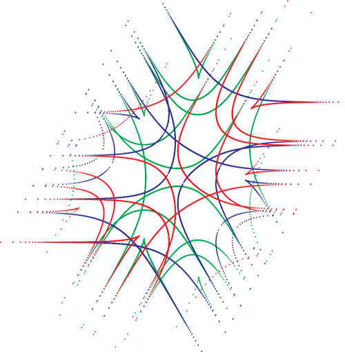
Figure 8: Images in the other three quadrants

Appendix A: Harnack curves and their algae.

In his 1876 paper [9] A. Harnack produced for each $d$ examples of algebraic curves of degree $d$ in ${\mathbb{R}}{\mathbb{P}}^{2}$ with $\frac{(d-1)(d-2)}{2}+1$ real (topological) components. Furthermore, in the same paper he has shown that $\frac{(d-1)(d-2)}{2}+1$ is the upper bound for the number of components of any curve of degree $d$ in ${\mathbb{R}}{\mathbb{P}}^{2}$

Among the curves constructed by Harnack there were some “canonical” curves whose topological arrangement in ${\mathbb{R}}{\mathbb{P}}^{2}$ is especially easy to describe. Note that any component of a smooth curve is either contractible (i.e. bounds a disk in ${\mathbb{R}}{\mathbb{P}}^{2}$) or is isotopic to ${\mathbb{R}}{\mathbb{P}}^{1}\subset{\mathbb{R}}{\mathbb{P}}^{2}$. A contractible component is called an oval while the disk bounded by it is called the interior of the oval. The oval whose interior is disjoint from other ovals is called empty.

For an odd $d=2k+1$ there is a smooth algebraic curve of degree $d$ that consists of $k(2k-1)$ empty ovals and a non-contractible component. For an even $d=2k$ there is a smooth algebraic curve of degree $d$ that consists of $(k-1)(2k-1)$ empty ovals and one other oval whose interior contains $\frac{(k-1)(k-2)}{2}$ of the $(k-1)(2k-1)$ empty ovals.

Let $P\subset\mathcal{T}$ be a curve given by a real polynomial with the Newton Polygon $\Delta_{P}$ and $\mathcal{T}$ be the toric surface corresponding to $\Delta_{P}$. Since $P$ is defined over $\mathbb{R}$ there is the real locus $\mathbb{R}P=P\cap(\mathbb{R}^{\times})^{2}$ which coincides with the fixed point set of the involution of complex conjugation on $P$.

Definition 6.5.

A curve $P$ is called a Harnack curve if for every $(x,y)\in\mathbb{R}^{2}$ the set $\operatorname{Log}^{-1}(x,y)\cap P$ consists of no more than two points.

Remark 6.6.

Earlier we called such curves simple Harnack curves to distinguish them from other curves in the Harnack construction. However, by now we have convinced ourselves that these simple curves are the most beautiful in the Harnack series of constructions. We propose to drop “simple” from their name and call them Harnack curves.

Harnack curves (from Definition 6.5) exist for any convex lattice polygon $\Delta$, cf. [10]. In [19] it was shown that the topological type of the triad $(\mathbb{R}\mathcal{T};\mathbb{R}P,\partial\mathbb{R}\mathcal{T})$ depends only on $\Delta$ if $\mathbb{R}P$ is a smooth Harnack curve transverse to infinity.

In the case when $\Delta$ is a triangle with vertices $(0,0)$, $(d,0)$ and $(0,d)$ we have $\mathbb{R}\mathcal{T}={\mathbb{R}}{\mathbb{P}}^{2}$ and $\mathbb{R}P\subset{\mathbb{R}}{\mathbb{P}}^{2}$ is a curve consisting of $\frac{(d-1)(d-2)}{2}$ empty oval and one other component which is non-contractible if $d$ is odd and an oval containing $\frac{(d-2)(d-4)}{8}$ empty ovals if $d$ is even. In [12] it was shown that all such curve form a contractible subspace in the space of all real curves of degree $d$.

Recently it was discovered that Harnack curves possess many extremal characteristic properties, among them are the following.

• ([21]) We have

  $$\operatorname{Area}(\operatorname{Log}(P))=\pi^{2}\operatorname{Area}(\Delta),$$

  if $\mathbb{R}P$ is a Harnack curve with the Newton polygon $\Delta$. In the same time by [24] for any curve $A\subset(\mathbb{C}^{\times})^{2}$ given by a (not necessarily real) polynomial with the Newton polygon $\Delta$ we have

  $$\operatorname{Area}(\operatorname{Log}(A))\leq\pi^{2}\operatorname{Area}(\Delta).$$

  Furthermore, if $\operatorname{Area}(\operatorname{Log}(A))=\pi^{2}\operatorname{Area}(\Delta)$ then $A$ can be translated (by a multiplication with some $(z_{0},w_{0})\in(\mathbb{C}^{\times})^{2}$) to a Harnack curve, see [21].

• ([19]) The curve $\operatorname{Log}(\mathbb{R}P)\subset\mathbb{R}^{2}$ is embedded, does not have inflection points and contains $\#(\operatorname{Int}(\Delta)\cap\mathbb{Z}^{2})$ compact components (called ovals) if $\mathbb{R}P$ is a Harnack curve. Each such oval comes from one of the four quadrants in $(\mathbb{R}^{\times})^{2}$. The number of the ovals coming from the four quadrant equals to the number of lattice points $(j,k)\in\mathbb{Z}^{2}$ in the interior $\operatorname{Int}(\Delta)$ with given residue mod 2: $j\equiv j_{0}\pmod{2}$, $k\equiv k_{0}\pmod{2}$ (clearly there are four possible pairs of residues).

  Furthermore any curve with that many ovals of $\operatorname{Log}(\mathbb{R}P)\approx P\smallsetminus\partial P$ is Harnack if the remaining component of $\mathbb{R}P$ intersects the infinity $\partial\mathbb{R}\mathcal{T}$ in a maximal way (see [19]).

The only singularities of a Harnack curve $\mathbb{R}P$ are isolated double points (the singularities of type $A_{1}^{+}$ according to [1]) in $(\mathbb{R}^{\times})^{2}$, see [21]. Note that even though $\mathbb{R}P$ has to be smooth near the boundary divisor $\partial\mathbb{R}\mathcal{T}$ it does not have to be transverse to the boundary divisor. An example of a singular simple Harnack curve of degree 6 in ${\mathbb{R}}{\mathbb{P}}^{2}$ which is not transverse to the boundary divisor is sketched in Figure 9.

Figure 9: A singular simple Harnack curve in ${\mathbb{R}}{\mathbb{P}}^{2}$ and its position with respect to the boundary divisor.

The goal of this appendix is to give yet another characteristic property of the Harnack curves in terms of their algae. Suppose that $P$ is a Harnack curve Recall that in the previous section we denoted with $\hat{P}$ the result of the real blowing up of $\tilde{P}$ at the points $\partial P$ and with

$$\operatorname{Alga}_{P}:\hat{P}\to T$$

such that $\operatorname{Alga}_{P}|_{\tilde{P}\smallsetminus\partial P}=\beta\circ\operatorname{Arg}|_{\tilde{P}\smallsetminus\partial P}$. Recall that $P_{0}=\operatorname{Alga}^{-1}_{P}(0_{T})$.

Lemma A 1.

If $P$ is a Harnack curve then the restriction of the map $\operatorname{Alga}_{P}$ to $\hat{P}\smallsetminus P_{0}$

$$\hat{P}\smallsetminus P_{0}\to T\smallsetminus\{0_{T}\}$$

is an unbranched covering of degree $2Area(\Delta_{P})$.

Proof.

The critical points of the map $\operatorname{Arg}|_{P}$ are the points such that the image of the Logarithmic Gauss map $\gamma_{P}$ is in ${\mathbb{R}}{\mathbb{P}}^{1}$ (see [19]). By [19] $\gamma^{-1}({\mathbb{R}}{\mathbb{P}}^{1})=\mathbb{R}\tilde{P}$. The map $\operatorname{Alga}_{P}|_{\hat{P}\smallsetminus P_{0}}$ is proper since $\operatorname{Alga}_{P}^{-1}(0_{T})=P_{0}$.

Since $\chi(T\smallsetminus\{0_{T}\})=-1$ we have the degree of the covering $\operatorname{Alga}_{P}|_{\hat{P}\smallsetminus P_{0}}$ equal to $-\chi(P\smallsetminus P_{0})$. Let us start with a generic $P$ and study how does $\chi(P\smallsetminus P_{0})$ changes when we deform $P$ in the class of Harnack curve. Since $P$ is a simple Harnack curve we have $P\smallsetminus P_{0}$ non-singular. The only singularities of $P$ are the real isolated double points. Each such point contributes $2$ to the Euler characteristic of the normalization of $P$, but also $2$ gets subtracted when we remove this point from $\hat{P}$.

Note that $P$ may also have the “boundary” singularity. This means that ${P}$ is not transversal to the boundary divisor. In this case each point of tangency of order $m$ between ${P}$ and $\partial\mathcal{T}$ gives $m-1$ points in $\hat{P}\smallsetminus P_{0}$. Thus, while $\chi(\hat{P})$ gets increased by $m-1$ in the case of such tangency (in comparison with $\chi(\hat{P})$ in the transversal case) in turn $\chi(\hat{P}\smallsetminus P_{0})$ gets decreased by $m-1$. Thus in both cases the net effect of possible singularities on $\chi(\hat{P}\smallsetminus P_{0})$ is zero, so for the computation of the degree of our covering we may assume that $\tilde{P}$ is smooth and transversal to the boundary divisor of $\mathcal{T}$. In this case

$$\chi(\hat{P}\smallsetminus P_{0})=\chi(\hat{P})=\chi(P)=\operatorname{Area}\Delta.$$

The last equality is a corollary of Khovanskii’s formula [15]. ∎

We may compactify the set-up of Lemma 1 to get the following Theorem describing the alga of a Harnack curve. Denote the blow-up of $T$ centered in $0_{T}$ with $B:\hat{T}\to T$.

Note that $\hat{T}$ is a surface with a natural involution induced by $\operatorname{conj}$: $(\alpha,\beta)\mapsto(-\alpha,-\beta)$, here we think of $\alpha,\beta\in S^{1}$ as arguments of complex numbers. Clearly, the 1-dimensional part of the fixed-point set of this involution is the exceptional divisor of the blow-up. Denote it with $\mathbb{R}\hat{T}$.

For the compactifying theorem we need to blow up $\hat{P}$ even further. Recall that $\hat{P}$ is a smooth (real) surface equipped with an involution coming from complex conjugation. Note that $0_{T}$ is the regular value of a map $P\smallsetminus\mathbb{R}P\to T$ and thus $P_{0}\subset\hat{P}$ is a disjoint union of embedded circles corresponding to the ovals of $\mathbb{R}\tilde{P}$ and some isolated points. Let $\Pi$ be the result of (real) blow-up of $\hat{P}$ at $P_{0}$. Clearly, a blow-up at a smooth submanifold of codimension 1 does not change the surface $\hat{P}$ thus only blowups at the isolated points of $P_{0}$ matter. Such points come either from isolated double points of $P$ or from tangency of $\tilde{P}$ with $\partial\mathcal{T}$. Note that

$$\chi(\Pi)=\chi(\hat{P}\smallsetminus P_{0}).$$

Theorem A 1.

There exists a map $p$ completing the commutative diagram

.

The map $p$ is a covering of degree $2\operatorname{Area}(\Delta_{P})$ which is equivariant with respect to the involution of complex conjugation defined on $\Pi$.

Furthermore, any real curve $P$ such that $\operatorname{Alga}_{P}$ lifts to a covering $\Pi\to\hat{T}$ is a Harnack curve.

Proof.

The point of $\mathbb{R}\hat{T}$ is specified by a tangent line to $T$ at $0_{T}$. The logarithmic Gauss map $\gamma_{P}$ takes real values at $\mathbb{R}\hat{P}$. Thus the tangent line at $s\in\mathbb{R}\hat{P}$ is real and gives (after multiplication by $i$) a tangent direction at $0_{T}\in T$. We define the value $p(s)$ to be this direction. At points of $P_{0}\smallsetminus\mathbb{R}\hat{P}$ the map is defined by the blowup itself (recall that $0_{T}$ is the regular value of the map $P\smallsetminus\mathbb{R}P\to T$).

For the converse we note that by [19] the amoeba map $\operatorname{Log}|_{P}$ does not have critical points outside of $\mathbb{R}P$ since $\operatorname{Alga}_{P}$ does not have any. Thus $\gamma_{P}$ cannot have any critical points on $\mathbb{R}P$.

∎

References

- [1] Arnold, V. I., Gusein-Zade, S. M., Varchenko, A. N., Singularities of differentiable maps. Vol. I. The classification of critical points, caustics and wave fronts. Monographs in Mathematics, 82. Birkha”user Boston, Inc., Boston, MA, 1985.
- [2] Bernstein, D.N., The number of roots of a system of equations. Functional Anal. Appl. 9 (1975), 183-185.
- [3] Brieskorn, E., Knörrer, H., Ebene algebraische Curven, Birkhäuser Verlag, Basel-Boston, 1981.
- [4] Coolidge, J.L., A treatise on algebraic plane curves, Dover Publications, Inc., New York 1959
- [5] Cohn, H., Larsen, M., Propp, J., The shape of a typical boxed plane partition, New York J. Math. 4 (1998), 137–165.
- [6] Gelfand I.M., Kapranov M.M., Zelevinsky A.V., Discriminants, resultants, and multidimensional determinants. Mathematics: Theory & Applications. Birkhäuser Boston, Inc., Boston, MA, 1994.
- [7] Faber, C., Okounkov, A., unpublished.
- [8] Feng, B., He Y.-H., Kennaway K. D., Vafa C., Dimer Models from Mirror Symmetry and Quivering Amoebae. hep-th/0511287
- [9] Harnack, A., Über die Vieltheiligkeit der ebenen algebraischen Curven, Math. Ann. 10 (1876), 189–199.
- [10] Itenberg, I., Viro O., Patchworking algebraic curves disproves the Ragsdale conjecture. Math. Intelligencer 18 (1996), no. 4, 19–28.
- [11] Kapranov, M.M., A characterization of -discriminantal hypersurfaces in terms of the logarithmic Gauss map, Math. Ann. 290 (1991), 277-285
- [12] Kenyon, R., Okounkov, A., Planar dimers and Harnack curves, math.AG/0311062.
- [13] Kenyon, R., Okounkov, A., Limit shapes and complex Burgers equation, math-ph/0507007.
- [14] Kenyon, R., Okounkov, A., Sheffield, S., Dimers and amoebae, math-ph/0311005.
- [15] Khovanskii, A.G., Newton polyhedra and toric varieties. Funktional. Anal. i Prilozhen., 11 (1977), no. 4, 56–64.
- [16] Klein, F., Eine neue Relation zwischen den Singularitäten einer algebraichen Curve, Math. Ann., 10 (1876) 199-210.
- [17] Klein, F., Elementarmathematik vom höheren Standpunkte aus. Zweiter Band: Geometrie, (German) Dritte Auflage. Springer-Verlag, Berlin 1968.
- [18] Kouchnirenko, A.G., Newton polytopes and the Bezout theorem, Functional Anal. Appl. 10 (1976), 233-235.
- [19] Mikhalkin, G., Real algebraic curves, the moment map and amoebas. Ann. of Math. (2) 151 (2000), no. 1, 309–326.
- [20] Mikhalkin, G., Amoebas of algebraic varieties and tropical geometry. Different faces of geometry, 257–300, Int. Math. Ser. (N. Y.), Kluwer/Plenum, New York, 2004.
- [21] Mikhalkin, G., Rullgård, H., Amoebas of maximal area. Internat. Math. Res. Notices 2001, no. 9, 441–451.
- [22] Milnor, J., Singular points of complex hypersurfaces, Annals of Mathematics Studies, No. 61 Princeton University Press, University of Tokyo Press 1968.
- [23] Passare, M., Amoebas, convexity and the volume of integer polytopes. Complex analysis in several variables—Memorial Conference of Kiyoshi Oka’s Centennial Birthday, 263–268, Adv. Stud. Pure Math., 42, Math. Soc. Japan, Tokyo, 2004.
- [24] Passare, M., Rullgård, H., Amoebas, Monge-Ampe‘re measures, and triangulations of the Newton polytope. Duke Math. J. 121 (2004), no. 3, 481–507.
- [25] Plücker, J., Solution d’une question fondamentale concernant la théorie generale des courbes, J. Reine Angew. Math., 12 (1834), 105-108.
- [26] Viro O.Ya., private communications.
- [27] Viro O.Ya., Some integral calculus based on Euler characteristic, Lecture Notes in Math., 1346 (1988), Springer, Berlin, 127-138.
- [28] Wall, C.T.C, Singular points of plane curves, Cambridge University Press, 2004.