Operator identities relating sonar and Radon transforms in Euclidean space

Abstract

We establish new relations which connect Euclidean sonar transforms (integrals taken over spheres with centers in a hyperplane) with classical Radon transforms. The relations, stated as operator identities, allow us to reduce the inversion of sonar transforms to classical Radon inversion.

1 Introduction

As we aim to relate sonar transforms with Radon transforms, we must begin by recalling key definitions which in turn requires us first to fix some notation. $\mathbb{R}_{+}^{n}:=\mathbb{R}^{n-1}\times(0,\infty)$ denotes the upper half space of $\mathbb{R}^{n}$. Points in $\mathbb{R}_{+}^{n}$ will be written as $(x,y)$ with $x\in\mathbb{R}^{n-1}$ and $y>0$. We write $|x|$ for the Euclidean vector norm of $x\in\mathbb{R}^{n-1},$ $dt$ for the Euclidean volume element on $\mathbb{R}^{n-1}$. $C_{c}^{\infty}\left(\mathbb{R}_{+}^{n}\right)$ (resp. $C^{\infty}\left(\mathbb{R}_{+}^{n}\right)$) denotes the set of smooth compactly supported functions (resp. smooth functions) on $\mathbb{R}^{n}$ supported in $\mathbb{R}_{+}^{n}$. $\mathbb{S}_{x,y}^{n-1}$ will denote the sphere in $\mathbb{R}^{n}$ centered at $x$ with radius $y$ (empty if $y<0$) carrying area measure $dS$.

We now define the sonar transform $\mathcal{S}:C_{c}^{\infty}\left(\mathbb{R}_{+}^{n}\right)\mapsto C^{\infty}\left(\mathbb{R}_{+}^{n}\right)$ as follows.

Definition 1.1.

Given $f\in C_{c}^{\infty}\left(\mathbb{R}_{+}^{n}\right)$,

$$\mathcal{S}[f](x,y):=\int_{\mathbb{S}_{x,y}^{n-1}}f\,dS.$$

The centerset variable $x$ parameterizes the centerset $\mathbb{R}^{n-1}\times\{0\}.$ On occasion we call $y$ the radial variable.

More explicitly,

$$\mathcal{S}[f](x,y)=\int_{|t|<y}f\left(x+t,\sqrt{y^{2}-|t|^{2}}\right)\,\frac{y\,dt}{\sqrt{y^{2}-|t|^{2}}}.$$ (1)

The sonar data $\mathcal{S}[f]$ generally does not have compact support. However the restriction of $\mathcal{S}[f]$ to any hyperplane parallel with the centerset is compactly supported which justifies various compositions of transforms below.

Remark 1.2.

While we restrict $\mathcal{S}$ to $C_{c}^{\infty}\left(\mathbb{R}_{+}^{n}\right)$ for the sake of our subsequent derivations, Definition 1.1 makes sense for locally integrable functions $f$.

Courant and Hilbert initiated the study of $\mathcal{S}$ in Methods of Mathematical Physics, Volume II [2], where they established its injectivity on the space of continuous functions and used the result to investigate hyperbolic partial differential equations. While [2] terms the mapping $\mathcal{S}$ “integrals over spheres centered in the plane,” our more efficient “sonar” terminology follows recent applications of $\mathcal{S}$ to marine tomography as in work of Louis and Quinto [8], where the operator $\mathcal{S}$ (in dimension three) models naval sonar data.

Operator $\mathcal{S}$ has other practical uses. As Cheney [1] explains, in dimension two $\mathcal{S}$ describes synthetic aperture radar. As $\mathcal{S}$ and its generalizations abstract the behavior of reflected waves (echoes) whether acoustic, electromagnetic, or mechanical, they play a central role in reflective tomography, including marine tomography and radar theory.

For the sake of recalling the classical Radon transform $\mathcal{R}$, we will write the set of all hyperplanes in a real vector space $V$ as ${\cal P}(V)$, which carries the structure of a smooth manifold. We now define $\mathcal{R}_{V}:C_{c}^{\infty}\left(V\right)\mapsto C_{c}^{\infty}\left({\cal P}(V)\right)$ as follows.

Definition 1.3.

$$\mathcal{R}_{V}[f](P):=\int_{P}f(x)\,dm_{x},$$

where $dm_{x}$ denotes planar surface measure on $P\in{\cal P}(V).$

For $V=\mathbb{R}^{n}$ we write the Radon transform simply as $\mathcal{R}$ whereas for $V=\mathbb{R}^{n-1}\times\{0\}\subset\mathbb{R}^{n}$ we denote the Radon transform $\overline{\mathcal{R}}$ and call it the centerset Radon transform. Note that both the sonar and Radon transforms reduce to the identity operator when $n=1$.

The operators $\mathcal{S}$ and $\mathcal{R}$ appear quite different conceptually. For example, Helgason [6] shows that the Radon transform has a very special group-theoretic structure which leads to the following inversion formula in $\mathbb{R}^{n}$ (taken from [6], p.15):

$$\frac{(4\,\pi)^{\frac{n-1}{2}}\,\Gamma\left(\frac{n}{2}\right)}{\Gamma\left(\frac{1}{2}\right)}\,f(x)=(-\Delta)^{\frac{n-1}{2}}\left(\mathcal{R}^{*}\circ\mathcal{R}\right)[f](x)$$ (2)

Here the superscript $*$ indicates the adjoint operator while $\Delta$ stands for the Laplacian. In odd dimensions, $(-\Delta)^{\frac{n-1}{2}}$ is a differential operator; in even dimensions, the fractional power of the negative Laplacian takes the form of a pseudodifferential operator that should be interpreted in terms of Riesz potentials.

In sharp contrast, the composition $\mathcal{S}^{*}\circ\mathcal{S}$ does not exist, as $\mathcal{S}[f]$ may lack compact support even when $f$ has one. And, despite the sonar transform’s sizable symmetry group (on $\mathbb{R}_{+}^{n}$, a semidirect product $O(n-1)\propto\mathbb{R}^{n-1}$ of the orthogonal group with translations), at present we lack a group-theoretic interpretation of $\mathcal{S}$.

In light of these differences, unexpected close relations between these two operators carry intrinsic interest. Denisjuk [3] found the first such relation:

Theorem 1.4 (Denisjuk, 1999).

$\mathbb{B}_{o,1}^{n}$ denotes the unit ball in $\mathbb{R}^{n}$. There exists a mapping $\phi:\mathbb{B}_{o,1}^{n}\mapsto\mathbb{R}_{+}^{n}$ (related to stereographic projection) and a certain non-negative weight $\sigma:\mathbb{B}_{o,1}^{n}\to\mathbb{R}$ such that for any smooth compactly supported function $f\in C_{c}^{\infty}\left(\mathbb{R}_{+}^{n}\right),$

$$\mathcal{S}[f]=\mathcal{R}[\sigma\cdot(f\circ\phi)].$$ (3)

Using Equation (3), Denisjuk expressed the inverse $\mathcal{S}^{-1}$ as a pull-back of the inverse Radon transform $\mathcal{R}^{-1}$ and established Plancherel identities for sonar. Theorem 1.4 was later used in [9] by Palamodov to pull back various microlocal estimates and perform $\Lambda$-type reconstruction on integrals over arcs. As both [3] and [9] demonstrate, sonar-Radon relations of type (3) can be effectively used to translate any Radon result into a corresponding sonar statement.

Denisjuk connects the sonar transform of a given function to the Radon transform of a different function with, a priori, a different support. Since $\mathbb{R}_{+}^{n}\subset\mathbb{R}^{n}$ and thus $C_{c}^{\infty}\left(\mathbb{R}_{+}^{n}\right)\subset C_{c}^{\infty}\left(\mathbb{R}^{n}\right),$ it makes sense to speak of the Radon transform and sonar transform of one and the same function $f$ (as long as $f$ has support in $\mathbb{R}_{+}^{n}$). This article addresses the following natural question:

How can one pass directly from the sonar transform of a function to its Radon transform?

A simplified version of our main result says that for almost all planes $P$, we can compute $\mathcal{R}[f](P)$ as

$$(\mathcal{W}\circ\mathcal{A}_{1/y}\circ\mathcal{D}_{\frac{n-2}{2}}\circ\overline{\mathcal{R}}\circ\mathcal{S})[f](P).$$

for certain explicitly described operators $\mathcal{W}$, $\mathcal{A}_{1/y}$, and $\mathcal{D}_{\frac{n-2}{2}}$ each of which has a natural geometric meaning.

2 Main Result

We aim to compute the function $\mathcal{R}[f]$ explicitly from the function $\mathcal{S}[f]$, the sonar data associated to $f$. In order to make our calculations as explicit as possible, we need a suitable parameterization of ${\cal P}(\mathbb{R}^{n})$. Our formula for calculating $\mathcal{R}[f](P)$, as it turns out, breaks into various cases depending on the geometry of the hyperplane $P$ relative to the centerset of the sonar transform. Accordingly, we write

$${\cal P}(\mathbb{R}^{n})=h\cup v\cup s,$$

a disjoint union, with

• the set of planes parallel to $\mathbb{R}^{n-1}$;

• the set of planes perpendicular to $\mathbb{R}^{n-1}$; and

• the set of all other planes (the slanted planes).

We shall write $\mathcal{R}^{(h)}[f]$, $\mathcal{R}^{(v)}[f]$, and $\mathcal{R}^{(s)}[f]$ for the corresponding restrictions of $\mathcal{R}[f]$ to $h$, $v$ and $s$.

To make matters more precise, we begin with a general parameterization of ${\cal P}$. To a pair $(\omega,p)$, $\omega\in\mathbb{S}_{o,1}^{n-1},$ $p\geq 0$, we may associate the hyperplane $P=\{x\in\mathbb{R}^{n}|\omega\cdot x=p\};$ here $\cdot$ denotes the standard inner product in $\mathbb{R}^{n}$. $P$ almost determines $(\omega,p)$; only if $p=0$, $\omega$ may vary by a sign.

Now we adapt this framework to take account of the centerset. We write $\omega=(\omega^{\prime},\omega_{n})\in\mathbb{R}^{n-1}\times\mathbb{R},$ and similarly $x=(x^{\prime},x_{n}).$ The equation $\omega\cdot x=p$ now takes the form $\omega^{\prime}\cdot x^{\prime}+\omega_{n}\,x_{n}=p.$ We can now distinguish three cases, as above:

• $\omega^{\prime}$ vanishes;

• $\omega_{n}$ vanishes;

• all others.

Start with $(h)$. Since $\omega\in\mathbb{S}_{o,1}^{n-1},$ we must have $\omega_{n}=\pm 1$. Dividing through by $\omega_{n}$, the defining equation of the plane has the form $x_{n}=y$ (for some appropriate $y$). The variable $y$ can now parameterize $(h)$. If $f\in C_{c}^{\infty}\left(\mathbb{R}_{+}^{n}\right)$ then

$$\mathcal{R}^{(h)}[f](y)=\int_{x\in\mathbb{R}^{n-1}}f(x,y)\,dx.$$ (4)

Thus we integrate over the centerset variable.

Now turn to $(v)$. A plane in $v$ has defining equation $\omega^{\prime}\cdot x^{\prime}=p.$ The intersection of a vertical plane with the centerset determines it, so parameterizing $v$ amounts to parameterizing the set of all hyperplanes in the centerset. As before, $P$ almost determines $(\omega^{\prime},p)$; only if $p=0$, $\omega^{\prime}$ may vary by a sign. Accordingly, we shall write

$$\mathcal{R}^{(v)}[f](\omega,p)=\int_{0}^{\infty}\left[\int_{\omega\cdot x=p}f(x,y)\,dm_{x}\right]\,dy$$ (5)

where $\omega=(\omega^{\prime},0)$. Observe that

$$\int_{\omega\cdot x=p}f(x,y)\,dm_{x}=\overline{\mathcal{R}}[f(\cdot,y)](\omega,p)$$ (6)

(which we view as an equality between functions of $y$), so we may also write Equation (5) as

$$\mathcal{R}^{(v)}[f](\omega,p)=\int_{0}^{\infty}\overline{\mathcal{R}}[f(\cdot,y)](\omega,p)\,dy.$$

The final case $(s)$ comprises a dense open subset of ${\cal P}(\mathbb{R}^{n})$, and thus makes the most substantial contribution to our union (provided $n>1$).

A plane in $(s)$ has defining equation $\omega^{\prime}\cdot x^{\prime}+\omega_{n}\,x_{n}=p$ with neither $\omega^{\prime}$ nor $\omega_{n}$ vanishing. We can scale this equation so as to normalize $\omega^{\prime}$ and simultaneously render the coefficient of $x_{n}$ negative. Thus we can unambiguously choose a defining equation for the same plane with

$$(\omega^{\prime},p,-\omega_{n})\in\mathbb{S}_{o,1}^{n-2}\times\mathbb{R}\times\mathbb{R}_{+}$$

Now the pair $(\omega^{\prime},p)$ by itself determines the intersection of $P$ with the centerset, so $\omega_{n}$ controls the angle between $P$ and the centerset. More explicitly, write $\omega_{n}=-\cot\beta$ with $\beta\in(0,\pi/2).$ Then the defining equation of the plane has the form

$$\omega^{\prime}\cdot x^{\prime}-\cot\beta\,x_{n}=p.$$

Intersecting with the parallel translate of the centerset where $x_{n}=s\,\sin\beta$ gives

$$\omega^{\prime}\cdot x^{\prime}=p+s\,\cos\beta.$$

Henceforth we parameterize $(s)$ by $(\omega^{\prime},p,\beta)$; $\beta$ now directly represents the angle between $P$ and the centerset.

Integration of $f\in C_{c}^{\infty}\left(\mathbb{R}_{+}^{n}\right)$ over $P$ can be split into integration over $P\cap\mathbb{R}^{n-1}$ followed by integration over $\beta$. Explicitly,

$$\mathcal{R}^{(s)}[f](\omega^{\prime},p,\beta)=\int_{0}^{\infty}\overline{\mathcal{R}}[f(\cdot,s\sin\beta)]\left(\omega,p+s\,\cos\beta\right)ds.$$ (7)

Remark 2.1.

We avoid including $(v)$ in $(s)$ as a special case $\beta=\pi/2$ both to get a good parameterization of $(s)$ and because the cases require separate treatment below.

Theorem 2.2 (Sonar-Radon relations in $\mathbb{R}_{+}^{n}$).

The sonar transform $\mathcal{S}[f]$ determines $\mathcal{R}[f]$ by means of the following operator identities:

$$\mathcal{R}^{(h)} = \mathcal{D}_{\frac{n-1}{2}}\circ\mathcal{R}^{(h)}\circ\mathcal{S},$$ (8)

$$\mathcal{R}^{(v)} = \mathcal{L}\circ\mathcal{S},$$ (9)

$$\mathcal{R}^{(s)} = \mathcal{W}\circ\mathcal{A}_{1/y}\circ\mathcal{D}_{\frac{n-2}{2}}\circ\overline{\mathcal{R}}\circ\mathcal{S}.$$ (10)

Here $\overline{\mathcal{R}}$ stands for the centerset Radon transform; $\mathcal{A}_{\sigma(y)}$ stands for the weighted Radon transform (38) from Definition 7.1 in Section 7; $\mathcal{D}_{\nu}$ and $\mathcal{W}$ denote fractional operators defined in Section 3 by (18) and (20), respectively; $\mathcal{L}$ represents an infinite limit defined in Section 7 by Equation (33).

We organize the proof as follows. Sections 3 and 4 contain necessary analytical tools: Section 3 details the fractional operators $\mathcal{D}_{\nu}$ and $\mathcal{W}$ (and their inverses); Section 4 collates identities for spherical integrals of plane waves from F. John’s classic Plane Waves and Spherical Means [7], for use in Section 8. Section 5 and 6 treat $\mathcal{R}^{(h)}$ and $\mathcal{R}^{(v)}$, respectively. Sections 7 and 8 treat $\mathcal{R}^{(s)}$ and thus complete the proof of our sonar-Radon relations: Section 7 motivates the choice of the weight $\sigma=1/y$ for operator $\mathcal{A}_{1/y}$ and establishes results in dimension two; Section 8 generalizes these results to higher dimensions. Section 9 analyzes the main result and offers closing remarks.

3 Fractional Calculus

We recall notions from fractional calculus, especially regarding operators $\mathcal{D}_{\nu}$ and $\mathcal{W}$ appearing in our sonar-Radon relations. The standing assumption that all fractional operators act on the last variable of smooth compactly supported functions will avoid those various delicate issues discussed at length by Samko et al in [10]. Compact support obviates potential divergence; smoothness ensures commutativity of operators.

As we choose to view the fractional integrals $\mathcal{I}_{\nu}$ as the fundamental fractional operators, we develop all other fractional operators out of these.

Definition 3.1.

For $\nu>0$ we define $\mathcal{I}_{\nu}$, a type of fractional integral, by

$$\mathcal{I}_{\nu}[g](y)=\frac{2\,\pi^{\nu}}{\Gamma(\nu)}\,y\,\int_{0}^{y}\left(y^{2}-s^{2}\right)^{\nu-1}\,g(s)\,ds.$$ (11)

For convenience, we also set $\mathcal{I}_{0}=\operatorname{id}.,$ the identity operator.

According to Lemma 3.2 below, the set $\left\{\mathcal{I}_{\nu}\right\}_{\nu=0}^{\infty}$ of fractional integral operators forms a monoid (semigroup with identity) under composition.

Lemma 3.2.

The fractional integrals in Definition 3.1 satisfy the composition law

$$\mathcal{I}_{\mu}\circ\mathcal{I}_{\nu}=\mathcal{I}_{\mu+\nu},$$ (12)

which holds for all $\mu,\nu\geq 0.$

Proof.

Equation (12) certainly holds if either $\mu=0$ or $\nu=0$ on account of the convention $\mathcal{I}_{0}=\operatorname{id}.$ So assume $\mu,\nu>0$.

Using Equation (11), we express the composition $(\mathcal{I}_{\mu}\circ\mathcal{I}_{\nu})[g](y)$ as an iterated integral

$$\frac{2\,\pi^{\mu}}{\Gamma(\mu)}\,\frac{2\,\pi^{\nu}}{\Gamma(\nu)}\,y\,\int_{0}^{y}\left(y^{2}-s^{2}\right)^{\mu-1}\,s\,\left[\int_{0}^{s}\left(s^{2}-t^{2}\right)^{\nu-1}\,g(t)\,dt\right]\,ds.$$ (13)

Changing the order of integration in (13) yields the following expression for $(\mathcal{I}_{\mu}\circ\mathcal{I}_{\nu})[g](y):$

$$\frac{2\,\pi^{\mu+\nu}}{\Gamma(\mu)\,\Gamma(\nu)}\,y\,\int_{0}^{y}\left[I(t)\right]\,g(t)\,dt.$$ (14)

where

$$I(t)=\int_{t}^{y}\left(y^{2}-s^{2}\right)^{\mu-1}\,\left(s^{2}-t^{2}\right)^{\nu-1}\,2s\,ds.$$ (15)

Substituting $s^{2}=\left(y^{2}-t^{2}\right)\,p+t^{2},$ gives

$$I(t)=C\left(y^{2}-t^{2}\right)^{\mu+\nu-1}$$

with the constant

$$C=\int_{0}^{1}(1-p)^{\mu-1}\,p^{\nu-1}\,dp$$

taking the form of Euler’s integral of the first kind (see [4] p.948 # 8.380.1) with value given by

$$C=\frac{\Gamma(\mu)\,\Gamma(\nu)}{\Gamma(\mu+\nu)}.$$

Thus

$$(\mathcal{I}_{\mu}\circ\mathcal{I}_{\nu})[g](y)=\frac{2\,\pi^{\mu+\nu}}{\Gamma(\mu)\,\Gamma(\nu)}\,y\,\int_{0}^{y}\left[\frac{\Gamma(\mu)\,\Gamma(\nu)}{\Gamma(\mu+\nu)}\left(y^{2}-t^{2}\right)^{\mu+\nu-1}\,\right]\,g(t)\,dt.$$ (16)

Cancelling four gamma terms, we obtain

$$(\mathcal{I}_{\mu}\circ\mathcal{I}_{\nu})[g](y)=\frac{2\,\pi^{\mu+\nu}}{\Gamma(\mu+\nu)}\,y\,\int_{0}^{y}\left(y^{2}-t^{2}\right)^{\mu+\nu-1}\,f(t)=\mathcal{I}_{\mu+\nu}[g](y)\,dt,$$

as desired. ∎

The justification for the terminology fractional integrals for the $\mathcal{I}_{\nu}$ rests on the semigroup property and the observation that

$$\mathcal{I}_{1}[g](y)=2\,\pi\,y\int_{0}^{y}g(s)\,ds,$$

a scaled antiderivative. Now $\mathcal{I}_{1}$ admits a left inverse in the form

$$\mathcal{D}_{1}[g](y):=\frac{1}{2\,\pi}\,\frac{d}{dy}\left[\frac{g(y)}{y}\right].$$ (17)

So, symbolically, we have $\mathcal{D}_{1}\circ\mathcal{I}_{1}=\mathcal{I}_{0}=\operatorname{id},$ and, more generally,

Lemma 3.3.

For all $\nu>1$, $\mathcal{D}_{1}\circ\mathcal{I}_{\nu}=\mathcal{I}_{\nu-1}.$

Proof.

Using Lemma 3.2 and the associativity of operator composition

$$\mathcal{D}_{1}\circ\mathcal{I}_{\nu}=\mathcal{D}_{1}\circ(\mathcal{I}_{1}\circ\mathcal{I}_{\nu-1})=(\mathcal{D}_{1}\circ\mathcal{I}_{1})\circ\mathcal{I}_{\nu-1}=\mathcal{I}_{\nu-1}.$$

∎

We will now use Lemmas 3.2 and 3.3 to construct fractional derivatives of arbitrary order.

Definition 3.4.

For $\nu>0$ the fractional derivative $\mathcal{D}_{\nu}$ is defined in terms of (11) and (17) as a mapping

$$\mathcal{D}_{\nu}=\mathcal{D}_{1}^{\lceil\nu\rceil}\circ\mathcal{I}_{\lceil\nu\rceil-\nu},$$ (18)

where $\lceil\nu\rceil$ is the smallest integer greater than or equal $\nu$. For consistency with Definition 3.1, we define $\mathcal{D}_{0}=\operatorname{id}.$

As an immediate consequence of Lemmas 3.2 and 3.3, we have the following corollary.

Corollary 3.5.

For $\nu\geq 0$ the fractional derivative $\mathcal{D}_{\nu}$ is the inverse of the fractional integral $\mathcal{I}_{\nu}$, i.e.: $\mathcal{D}_{\nu}\circ\mathcal{I}_{\nu}=\operatorname{id}.$

In Section 7, we will encounter a fractional operator $\mathcal{V}$ and require its inverse $\mathcal{W}$ to deduce Equation (10) in Theorem 2.2.

Definition 3.6.

Set

$$\mathcal{V}[g](\beta):=\int_{0}^{\beta}\frac{2\,\sin\beta}{\sqrt{\sin^{2}\beta-\sin^{2}\theta}}\,g(\theta)\,d\theta.$$ (19)

From the definitions of $\mathcal{I}_{\frac{1}{2}}$ and $\mathcal{V}$

$$\mathcal{I}_{\frac{1}{2}}[g](\sin\beta)=\mathcal{V}[\cos\beta\,g(\sin\beta)](\beta).$$

We now cast this identity of functions as an identity of operators. Define ${\cal Q}[g](\beta):=g(\sin\beta)$ and ${\cal K}[g](\beta):=\cos\beta\cdot g(\sin\beta).$ Then the identity above says

$${\cal Q}\circ\mathcal{I}_{\frac{1}{2}}=\mathcal{V}\circ{\cal K}.$$

Thus

$$\mathcal{W}:=\mathcal{V}^{-1}={\cal K}\circ\mathcal{D}_{\frac{1}{2}}\circ{\cal Q}^{-1}.$$

Lemma 3.7.

$$\mathcal{W}[g](\beta):=\frac{1}{\pi}\,\frac{d}{d\beta}\int_{0}^{\beta}\frac{\cos\theta}{\sqrt{\sin^{2}\beta-\sin^{2}\theta}}\,g(\theta)\,d\theta$$ (20)

Proof.

We apply the composition of operators ${\cal K}\circ\mathcal{D}_{\frac{1}{2}}\circ{\cal Q}^{-1}$ to a function $g$. First,

$${\cal Q}^{-1}[g](s)=g(\arcsin s).$$

Next we use Equation (18) to write

$$\begin{split}({\mathcal{D}_{\frac{1}{2}}\circ\cal Q}^{-1})[g](\beta)&=(\mathcal{D}_{1}\circ\mathcal{I}_{\frac{1}{2}}\circ{\cal Q}^{-1})[g](\beta)\\ &=\frac{1}{2\,\pi}\,\frac{d}{d\beta}\left[\frac{1}{\beta}\cdot 2\,\beta\int_{0}^{\beta}\frac{g(\arcsin s)}{\sqrt{\beta^{2}-s^{2}}}\,ds\right]\\ &=\frac{1}{\pi}\,\frac{d}{d\beta}\int_{0}^{\beta}\frac{g(\arcsin s)}{\sqrt{\beta^{2}-s^{2}}}\,ds\end{split}$$

Finally, we apply the operator $K$, which replaces $\beta$ with $\sin\beta$ and multiplies the result by $\cos\beta$, to get

$$\begin{split}({K\circ\mathcal{D}_{\frac{1}{2}}\circ\cal Q}^{-1})[g](\beta)&=\cos\beta\,\frac{1}{\pi}\,\frac{d}{d(\sin\beta)}\int_{0}^{\sin\beta}\frac{g(\arcsin s)}{\sqrt{\sin^{2}\beta-s^{2}}}\,ds\end{split}$$

whereupon the substitution $s=\sin\theta$ yields the statement of the lemma. ∎

4 Plane waves and spherical means

The identities for integrals over spheres and balls in $\mathbb{R}^{n}$ collected here, combined with the formulae from Section 3, form the crux of the derivations presented in Sections 5 and 8. In particular, we state the Co-area Formula, following [5], and develop some of its consequences.

Theorem 4.1 (Co-area formula).

Let $u:\mathbb{R}^{n}\mapsto\mathbb{R}$ be Lipschitz continuous and assume that for almost every $r\in\mathbb{R}$ the level set

$$\left\{x\in\mathbb{R}^{n}\,|\,u(x)=r\right\}$$

is a smooth, $(n-1)$-dimensional surface in $\mathbb{R}^{n}$. Suppose that also $g:\mathbb{R}^{n}\mapsto\mathbb{R}$ is continuous and locally integrable. Then

$$\int_{x\in\mathbb{R}^{n}}g\cdot|\operatorname{grad}u|\,dx=\int_{-\infty}^{\infty}\left[\int_{\{u=r\}}g\,dS\right]\,dr,$$ (21)

where $dS$ denotes surface measure on the level set $\{u=r\}.$

By setting $u=|x|$ in Theorem 4.1, one obtains a standard identity for converting integrals over balls into integrals over spheres in $\mathbb{R}^{n}$ which we state in Lemma 4.2.

Lemma 4.2 (Polar Coordinates).

Let $g:\mathbb{B}_{o,r}^{n}\mapsto\mathbb{R}$ be a continuous function on a ball of radius $r$ in Euclidean space. Then

$$\int_{|x|<r}g(x)\,dx=\int_{0}^{r}\left[\int_{x\in\mathbb{S}_{o,p}^{n-1}}f(x)\,dS_{x}\right]\,dp,$$ (22)

where $dS_{x}$ denotes surface measure on the sphere $\mathbb{S}_{o,p}^{n-1}$ of radius $p$.

Differentiating Equation (22) gives rise to the following.

Corollary 4.3.

Let $g:\mathbb{B}_{o,R}^{n}\mapsto\mathbb{R}$ be a continuous function. Then

$$\frac{d}{dr}\,\int_{x\in\mathbb{B}_{o,r}^{n}}g(x)\,dx=\int_{x\in\mathbb{S}_{o,r}^{n-1}}g(x)\,dS_{x}$$ (23)

holds for all $0<r<R.$

Often it is convenient to replace integration over a sphere of radius $r$ with integration over a unit sphere. As we remark below, this can be accomplished through a simple substitution.

Remark 4.4.

Let $g:\mathbb{S}_{o,r}^{n}\mapsto\mathbb{R}$ be a continuous function on a sphere of radius $r$. Then

$$\int_{x\in\mathbb{S}_{o,r}^{n-1}}g(x)\,dS_{x}=r^{n-1}\,\int_{\theta\in\mathbb{S}_{o,1}^{n-1}}g(r\,\theta)\,d\Omega_{\theta},$$ (24)

where $d\Omega_{\theta}$ is the surface measure on a unit sphere.

Using Remark 4.4, we recast Equation (22) in the form we shall find most useful:

$$\int_{|x|<r}g(x)\,dx=\int_{0}^{r}s^{n-1}\,\left[\int_{\theta\in\mathbb{S}_{o,1}^{n-1}}g(s\,\theta)\,d\Omega_{\theta}\right]\,ds.$$ (25)

Throughout the rest of this section $g$ denotes a continuous function of a scalar variable. Fix $v\in\mathbb{R}^{n}.$ Following F. John in [7], we call $G(x):=g(v\cdot x)$ a plane wave with normal $v$; such a function is constant on planes perpendicular to $v$.

We follow F. John in [7] to reduce integrals of plane waves over spheres and balls to single-dimensional integrals. On the plane $v\cdot x=|v|\,p$ the plane wave $g(v\cdot x)$ has constant value $g(|v|\,p)$; the intersection of that plane with the ball of radius $r$ forms a ball of radius $\sqrt{r^{2}-p^{2}}$. Thus

$$\begin{split}\int_{|x|<r}g(v\cdot x)\,dx&=\,\int_{-r}^{+r}\makebox{\rm Vol}(\mathbb{B}_{o,\sqrt{r^{2}-p^{2}}}^{n-1})g(|v|\,p)\,dp\\ &=\frac{|\mathbb{S}_{o,1}^{n-2}|}{n-1}\,\int_{-r}^{+r}\left(r^{2}-p^{2}\right)^{\frac{n-1}{2}}\,g(|v|\,p)\,dp.\end{split}$$ (26)

where $|\mathbb{S}_{o,1}^{n-2}|$ denotes the total surface measure of a unit sphere in $\mathbb{R}^{n-1}$. Differentiation of Equation (26) with respect to $r$ followed by evaluation at $r=1,$ leads to the following fundamental identity (c.f. [7], p.8).

Theorem 4.5.

Let $v\in\mathbb{R}^{n}$ be a fixed vector and let $g:\mathbb{R}\mapsto\mathbb{R}$ be a continuous function. Then

$$\int_{\theta\in\mathbb{S}_{o,1}^{n-1}}g(v\cdot\theta)\,d\Omega_{\theta}=|\mathbb{S}_{o,1}^{n-2}|\,\int_{-1}^{+1}\left(1-p^{2}\right)^{\frac{n-3}{2}}\,g(|v|\,p)\,dp.$$ (27)

We state two consequences of Theorem 4.5. If $v$ has unit length, then Equation (27) becomes an identity for “spherical plane waves” :

Corollary 4.6.

Let $\omega\in\mathbb{S}_{o,1}^{n-1}$ be a fixed point on a unit sphere in $\mathbb{R}^{n}$ and let $g:\mathbb{R}\mapsto\mathbb{R}$ be a continuous function. Then

$$\int_{\theta\in\mathbb{S}_{o,1}^{n-1}}g(\omega\cdot\theta)\,d\Omega_{\theta}=|\mathbb{S}_{o,1}^{n-2}|\,\int_{-1}^{+1}\left(1-p^{2}\right)^{\frac{n-3}{2}}\,g(p)\,dp.$$ (28)

Alternatively, on setting $g=1$, Theorem 4.5 gives a recursion for the total measure of a unit sphere (c.f. [7], p.9). From this recursion follows the well-known surface area formula:

$$|\mathbb{S}_{o,1}^{n-1}|=\frac{2\,\pi^{\frac{n}{2}}}{\Gamma\left(\frac{n}{2}\right)}.$$ (29)

We shall use this formula to connect our fractional integrals with geometric transforms.

5 Integrals over horizontal planes

We now prove Equation (4) of our Main Theorem:

$$\mathcal{R}^{(h)}=\mathcal{D}_{\frac{n-1}{2}}\circ\mathcal{R}^{(h)}\circ\mathcal{S}.$$

Since $\mathcal{D}_{\nu}$ inverts the fractional integral $\mathcal{I}_{\nu}$, it suffices to show that

$$\mathcal{R}^{(h)}\circ\mathcal{S}=\mathcal{I}_{\frac{n-1}{2}}\circ\mathcal{R}^{(h)}.$$ (30)

We compare $(\mathcal{R}^{(h)}\circ\mathcal{S})[f]$ with $(\mathcal{I}_{\frac{n-1}{2}}\circ\mathcal{R}^{(h)})[f]$ for $f\in C_{c}^{\infty}\left(\mathbb{R}_{+}^{n}\right).$ Directly from the definitions of the operators $\mathcal{S}$ and $\mathcal{R}^{(h)}$ (Equations (1),(4))

$$(\mathcal{R}^{(h)}\circ\mathcal{S})[f](y)=\int_{x\in\mathbb{R}^{n-1}}\left[\int_{|t|<y}f\left(x+t,\sqrt{y^{2}-|t|^{2}}\right)\,\frac{y\,dt}{\sqrt{y^{2}-|t|^{2}}}\right]\,dx$$

which, upon interchanging the order of integration, equals

$$\int_{|t|<y}\left[\int_{x\in\mathbb{R}^{n-1}}f\left(x+t,\sqrt{y^{2}-|t|^{2}}\right)\,dx\right]\,\frac{y\,dt}{\sqrt{y^{2}-|t|^{2}}}.$$

We recognize the inner integral as $\mathcal{R}^{(h)}[f](\sqrt{y^{2}-|t|^{2}})$ and deduce

$$\left(\mathcal{R}^{(h)}\circ\mathcal{S}\right)[f](y)=\int_{|t|<y}\mathcal{R}^{(h)}[f]\left(\sqrt{y^{2}-|t|^{2}}\right)\,\frac{y\,dt}{\sqrt{y^{2}-|t|^{2}}}.$$ (31)

The right-hand side of Equation (31) is an integral over a ball in $\mathbb{R}^{n-1}$ whose integrand

$$\mathcal{R}^{(h)}[f]\left(\sqrt{y^{2}-|t|^{2}}\right)\,\frac{y}{\sqrt{y^{2}-|t|^{2}}}$$

is a radial function of $t$. Therefore, using Equation (25) from Section 4, we rewrite Equation (31) in the form

$$|\mathbb{S}_{o,1}^{n-2}|\,y\,\int_{0}^{y}\frac{\mathcal{R}^{(h)}[f]\left(\sqrt{y^{2}-r^{2}}\right)}{\sqrt{y^{2}-r^{2}}}\,r^{n-2}\,dr,$$

which, after substituting $r=\sqrt{y^{2}-s^{2}}$ becomes

$$|\mathbb{S}_{o,1}^{n-2}|\,y\,\int_{0}^{y}\left(y^{2}-s^{2}\right)^{\frac{n-3}{2}}\mathcal{R}^{(h)}[f](s)\,ds=(\mathcal{I}_{\frac{n-1}{2}}\circ\mathcal{R}^{(h)})[f]$$ (32)

by Definition 3.1 in Section 3 and (29).

6 Integrals over vertical planes

Figure 1 suggests viewing a vertical hyperplane as a limiting case of expanding tangent spheres with a fixed point of tangency located on the centerset.

Accordingly,

$$\mathcal{R}^{(v)}[g](\omega,p)=\lim_{|s|\to\infty}\mathcal{S}[g](\omega\,s,|s-p|).$$

If we make the definition

$$\mathcal{L}[f](\omega,p):=\lim_{|s|\to\infty}f(\omega s,|p-s|).$$ (33)

then $\mathcal{R}^{(v)}=\mathcal{L}\circ\mathcal{S},$ as desired.

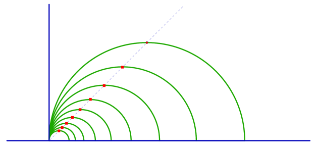
Figure 1: Vertical rays as limits of arcs

7 Integrals over slanted lines

In $\mathbb{R}_{+}^{2}$, our desired sonar-Radon relation Equation (10) reduces to:

$$\mathcal{R}^{(s)}=\mathcal{W}\circ\mathcal{A}_{1/y}\circ\overline{\mathcal{R}}\circ\mathcal{S}.$$ (34)

(As $\mathcal{D}_{\frac{n-2}{2}}=\mathcal{D}_{0}=\operatorname{id},$ no fractional derivative appears.) Below, this formula emerges as the foundation for the general case.

In dimension two, the centerset has dimension one. As hyperplanes in dimension one coincide with points, just in this section we will encode them as such (rather than as pairs of a unit vector and a magnitude). With this encoding the centerset Radon transform $\overline{\mathcal{R}}$ reduces to the identity map, so we must prove that

$$\mathcal{R}^{(s)}=\mathcal{W}\circ\mathcal{A}_{1/y}\circ\mathcal{S}.$$ (35)

Applying $\mathcal{V}$, the inverse of $\mathcal{W}$ to both sides yields the equivalent statement

$$\mathcal{V}\circ\mathcal{R}^{(s)}=\mathcal{A}_{1/y}\circ\mathcal{S}$$ (36)

for which we will aim.

Dimension two affords us a simple formula for the sonar transform:

$$\mathcal{S}[f](x,y)=\int_{0}^{\pi}f(x+y\,\cos\phi,y\,\sin\phi)\,y\,d\phi.$$ (37)

We now furnish the definition of $\mathcal{A}_{\sigma}$ — a type of weighted Radon transform on $\mathbb{R}_{+}^{2}$.

Definition 7.1.

Fix any set $T$. Consider a function $g$ on $T\times\mathbb{R}_{+}^{2}$ such that $g(\omega,\cdot)\in C_{c}^{\infty}\left(\mathbb{R}_{+}^{2}\right)$ for each $\omega$ in $T$. For $\beta\in(0,\pi/2)$ and non-negative weight $\sigma:\mathbb{R}_{+}\mapsto\mathbb{R}_{+},$ define a weighted Radon transform by

$$\mathcal{A}_{\sigma}[g](\omega,p,\beta)=\int_{0}^{\infty}g\left(\omega,p+s,s\,\sin\beta\right)\,\sigma(s)\,ds.$$ (38)

This section has $T$ a singleton and we thus suppress the variable $\omega$.

Consider the composition $\mathcal{A}_{\sigma}\circ\mathcal{S}$ for a general weight $\sigma$. $\mathcal{S}[f](p,y)$ means the integral of $f$ over over a radius $y$ circle centered at $p$ on the $x$-axis. By definition, the operator $\mathcal{A}_{\sigma}$ integrates functions along rays with slope $\sin\beta$. This makes $\mathcal{A}_{\sigma}[\mathcal{S}[f]\,](p,\beta)$ a weighted integral of integrals of $f$ over a family of circles, as in Figure 2.

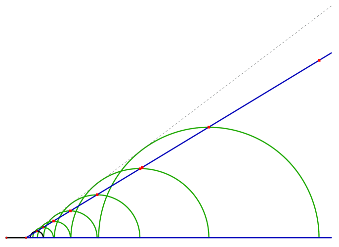
Figure 2: Semicircles tangential to a ray

One also sees from the figure that arcs with apexes on slanted rays sweep infinite wedges. If the apexes lie on a ray with slope $\sin\beta$ then the corresponding wedge has slope $\tan\beta$. Therefore $\mathcal{A}_{\sigma}[\mathcal{S}[f]\,](p,\beta)$ can be expressed as an integral over an infinite wedge with vertex at $p$ on the $x$-axis and angular measure $\beta$. Explicitly, by means of Equations (37) and (38),

$$\begin{split}&\mathcal{A}_{\sigma}[\mathcal{S}[f]\,](p,\beta)\\ &=\int_{0}^{\infty}\left[\int_{0}^{\pi}f\left(p+t\,(1+\sin\beta\,\cos\phi),t\,\sin\beta\,\sin\phi\right)\,d\phi\right]\,t\,\sin\beta\,\sigma(t)\,dt\end{split}$$ (39)

We now make a change of variables designed to simplify the argument of $f$ in Equation (39). Define $\Psi:\mathbb{R}^{2}\rightarrow\mathbb{R}^{2}$ by

$$\left[\begin{array}[]{c}\phi\\ t\\ \end{array}\right]\stackrel{{\scriptstyle\Psi}}{{\mapsto}}\left[\begin{array}[]{c}p+t\,(1+\sin\beta\,\cos\phi)\\ t\,\sin\beta\,\sin\phi\\ \end{array}\right].$$

Observe that $\Psi$ sends a line segment connecting $(0,t)$ and $(\pi,t)$ to the semicircle centered at $(p+t,0)$ with radius $t\sin\beta$.

On each of the two semi-infinite strips

$$\left(0,\frac{\pi}{2}+\beta\right)\times(0,\infty)\quad\text{and}\quad\left(\frac{\pi}{2}+\beta,\pi\right)\times(0,\infty)$$

$\Psi$ acts as a diffeomorphism to the infinite wedge

$$\left\{(x,y)\in\mathbb{R}^{2}\mid p<x,0<y<\tan\beta\,(x-p)\right\}$$

shown on Figure 2. In terms of $\Psi$, the double integral (39) over a wedge can be written as a sum of two integrals over infinite strips

$$\begin{split}&\int_{0}^{\infty}\left[\int_{0}^{\frac{\pi}{2}+\beta}(f\circ\Psi)(\phi,t)\,d\phi\right]\,t\,\sin\beta\,\sigma(t)\,dt\\ &+\int_{0}^{\infty}\left[\int_{\frac{\pi}{2}+\beta}^{\pi}(f\circ\Psi)(\phi,t)\,d\phi\right]\,t\,\sin\beta\,\sigma(t)\,dt.\end{split}$$ (40)

Introducing polar coordinates $(\rho,\theta)$, $\rho\in(0,\infty)$, $\theta\in(0,\beta)$ in the wedge

$$(p+t\,(1+\sin\beta\,\cos\phi),t\,\sin\beta\,\sin\phi)=(p+\rho\,\cos\theta,\rho\,\sin\theta)$$

gives us the relations:

$$t\,(1+\sin\beta\,\cos\phi) =\rho\,\cos\theta$$ (41)

$$t\,\sin\beta\,\sin\phi =\rho\,\sin\theta.$$ (42)

Using (41) and (42), we shall now change (40) into a much more amenable expression.

In order to transform (40), we need to express the old variables $(\phi,t)$ in terms of the new variables $(\theta,\rho)$ and find the corresponding Jacobian factors: one for each integral in (40). From the algebraic point of view, it is easier to find $\phi$. Divide Equation (42) by Equation (41): this eliminates variables $\rho$ and $t$. Next use trigonometric identities to solve the resulting relation between angles as follows:

$$\begin{split}\frac{\operatorname{Eq.}\eqref{e:r2r1polary}}{\operatorname{Eq.}\eqref{e:r2r1polarx}}&\Rightarrow\frac{\sin\beta\,\sin\phi}{1+\sin\beta\,\cos\phi}=\tan\theta\\ &\Rightarrow\sin\beta\,\sin\phi\,\cos\theta=\sin\theta+\sin\beta\,\cos\phi\,\sin\theta\\ &\Rightarrow\sin\phi\,\cos\theta-\cos\phi\,\sin\theta=\frac{\sin\theta}{\sin\beta}\\ &\Rightarrow\sin(\phi-\theta)=\frac{\sin\theta}{\sin\beta}\\ &\text{we get two solutions:}\\ &\left\{\begin{split}\phi_{1}&=\theta+\sin^{-1}\left(\frac{\sin\theta}{\sin\beta}\right),\\ \phi_{2}&=\theta+\pi-\sin^{-1}\left(\frac{\sin\theta}{\sin\beta}\right)\end{split}\right\}.\end{split}$$ (43)

With these expressions for the angular variable $\phi$, we may now find the corresponding values of $t$ as outlined in Equation (44) below:

$$\begin{split}\operatorname{Eq.}\eqref{e:r2r1polarx}\times\cos\theta&+\operatorname{Eq.}\eqref{e:r2r1polary}\times\sin\theta\\ &\Rightarrow t\,\cos\theta+t\,\sin\beta\,(\cos\phi\,\cos\theta+\sin\phi\,\sin\theta)=\rho\\ &\Rightarrow t\,\cos\theta+t\,\sin\beta\,\cos(\phi-\theta)=\rho\\ &\Rightarrow t=\frac{\rho}{\cos\theta+\sin\beta\,\cos(\phi-\theta)}\\ &\text{using the identity following from Equation \eqref{e:r2r1phi}:}\\ &\left(\begin{split}\sin\beta\,\cos(\phi-\theta)=\pm\sin\beta\,\sqrt{1-\sin^{2}(\phi-\theta)}&=\\ \pm\sin\beta\,\sqrt{1-(\sin^{2}\theta/\sin^{2}\beta)}=\pm\sqrt{\sin^{2}\beta-\sin^{2}\theta}\end{split}\right)\\ &\text{we get two solutions:}\\ &\left\{\begin{split}t_{1}&=\frac{\rho}{\cos\theta+\sqrt{\sin^{2}\beta-\sin^{2}\theta}},\\ t_{2}&=\frac{\rho}{\cos\theta-\sqrt{\sin^{2}\beta-\sin^{2}\theta}}\end{split}\right\}.\end{split}$$ (44)

Remark 7.2.

The relation between $(\phi,t)$ and $(\theta,\rho)$ can also be derived geometrically.

Figure 3: Polar coordinates

Consider semicircles inscribed in a fixed wedge of angular measure $\beta$ as in Figure 3. Our old variables $(\phi,t)$ specify a semicircle and then a point $B$ on it: from $t=OA$ we learn the center of the semicircle, and then from the tangency also its radius; $\phi$ locates the point $B$ since $\angle OAB=\pi-\phi$. From the right triangle $\triangle OAC$, we find the radius of the semicircle $r=t\,\sin\beta.$ A ray issuing from $O$ at angle $\theta<\beta$ with $OA$ will meet the semicircle twice and we take $B$ as the second intersection. The Law of Sines applied to triangle $\triangle OAB$ gives:

$$\frac{\sin(\angle AOB)}{AB}=\frac{\sin(\angle OBA)}{OA}\Rightarrow\frac{\sin\theta}{t\,\sin\beta}=\frac{\sin(\phi-\theta)}{t},$$

which is equivalent to (43). Then the Law of Cosines, in the form

$$OA^{2}+AB^{2}-2\,OA\,AB\,\cos(\angle OAB)=OB^{2},$$

tells us

$$t^{2}+t^{2}\,\sin^{2}\beta-2\,t^{2}\,\sin\beta\,\cos(\pi-\phi)=\rho^{2}.$$

After simplification (44) results.

As follows from Equation (43) the angular variable $\phi$ does not depend on $\rho$. Therefore the $2$-by-$2$ Jacobian matrix is triangular and its determinant is given by

$$\det\left[\begin{array}[]{cc}\frac{\partial\phi}{\partial\theta}&0\\ \frac{\partial t}{\partial\theta}&\frac{\partial t}{\partial\rho}\\ \end{array}\right]=\frac{\partial\phi}{\partial\theta}\times\frac{\partial t}{\partial\rho}.$$

The values of the partial derivatives $\frac{\partial\phi_{i}}{\partial\theta}$ and $\frac{\partial t_{i}}{\partial\rho}$ for $i=1,2$ can be found through straightforward differentiation:

$$\frac{\partial\phi_{i}}{\partial\theta} =1+\frac{(-1)^{i}}{\sqrt{1-(\sin^{2}\theta/\sin^{2}\beta)}}\,\frac{\cos\theta}{\sin\beta}=\frac{\sqrt{\sin^{2}\beta-\sin^{2}\theta}+(-1)^{i}\cos\theta}{\sqrt{\sin^{2}\beta-\sin^{2}\theta}},$$

$$\frac{\partial t_{i}}{\partial\rho} =\frac{1}{\cos\theta+(-1)^{i}\sqrt{\sin^{2}\beta-\sin^{2}\theta}},\quad i=1,2,$$

whence follows that for both sets of variables $(\phi_{1},t_{i})$ $i=1,2$ the absolute value of the determinant of the Jacobian is given by the same simple expression

$$\frac{1}{\sqrt{\sin^{2}\beta-\sin^{2}\theta}}.$$

We conclude that (40) can be written as a single integral of the form

$$\int_{0}^{\beta}\left[\int_{0}^{\infty}\frac{\sin\beta\,\left\{t_{1}\,\sigma(t_{1})+t_{2}\,\sigma(t_{2})\right\}}{\sqrt{\sin^{2}\beta-\sin^{2}\theta}}\,f(p+\rho\,\cos\theta,\rho\,\sin\theta)\,d\rho\right]\,d\theta,$$ (45)

where the values of $t_{i}$, $i=1,2$ in the numerator are given by (44).

Integral (45), representing the composition $\left(\mathcal{A}_{\sigma(y)}\circ\mathcal{S}\right)$ applied to $f$, becomes particularly simple if one sets the weight $\sigma=1/y:$

$$\begin{split}&\int_{0}^{\beta}\left[\int_{0}^{\infty}\frac{2\,\sin\beta}{\sqrt{\sin^{2}\beta-\sin^{2}\theta}}\,f(p+\rho\,\cos\theta,\rho\,\sin\theta)\,d\rho\right]\,d\theta\\ &=\int_{0}^{\beta}\frac{2\,\sin\beta}{\sqrt{\sin^{2}\beta-\sin^{2}\theta}}\,\left[\int_{0}^{\infty}f(p+\rho\,\cos\theta,\rho\,\sin\theta)\,d\rho\right]\,d\theta.\end{split}$$ (46)

Recognizing the bracketed integral as $\mathcal{R}^{(s)}$ (via Equation (7) from Section 2) and noticing that the outside integral is the fractional operator $\mathcal{V}$ (Definition 3.6 from Section 3), we get

$$\begin{split}(\mathcal{A}_{1/y}\circ\mathcal{S})[f](p,\beta)&=\int_{0}^{\beta}\frac{2\,\sin\beta}{\sqrt{\sin^{2}\beta-\sin^{2}\theta}}\,\mathcal{R}^{(s)}{f}(p,\theta)\,d\theta\\ &=(\mathcal{V}\circ\mathcal{R}^{(s)})[f](p,\beta),\end{split}$$

as desired.

8 Integrals over slanted planes

We now prove in all dimensions the sonar-Radon relation (10) first stated in Theorem 2.2 and reproduced below:

$$\mathcal{R}^{(s)}=\mathcal{W}\circ\mathcal{A}_{1/y}\circ\mathcal{D}_{\frac{n-2}{2}}\circ\overline{\mathcal{R}}\circ\mathcal{S}.$$

After some work, we reduce to the two-dimensional case treated in Section 7. Effectively, our conversion of sonar data into integrals over hyperplanes proceeds through an intermediate stage—integrals over cylinders.

In the usual way, let $(\omega,p)$ encode a hyperplane in the centerset of $\mathbb{R}_{+}^{n}$. By a cylinder, with radius $r$ with axis $(\omega,p)$, we mean any set:

$$\left\{(x,y)\in\mathbb{R}_{+}^{n}\mid(\omega\cdot x-p)^{2}+y^{2}=r^{2}\right\}.$$

We encode a cylinder of radius $y$ as a triple $(\omega,p,y)$ and write ${\cal C}[f](\omega,p,y)$ for the integral of $f$ over the given cylinder. (One naturally views transform ${\cal C}$ as a hybrid of sonar and Radon.) Given $\mathcal{S}[f]$, we can find ${\cal C}[f](\omega,p,y)$ as follows.

Theorem 8.1.

For $f\in C_{c}^{\infty}\left(\mathbb{R}_{+}^{n}\right),$

$${\cal C}[f](\omega,p,y)=(\mathcal{D}_{\frac{n-2}{2}}\circ\overline{\mathcal{R}}\circ\mathcal{S})[f](\omega,p,y)$$ (47)

Proof.

We shall actually prove the equivalent claim $\mathcal{I}_{\frac{n-2}{2}}\circ{\cal C}=\overline{\mathcal{R}}\circ\mathcal{S}$. Combining Equation (1) from Section 1 with Equation (6) from Section 2, we obtain an iterated integral for $(\overline{\mathcal{R}}\circ\mathcal{S})[f](\omega,p,y)$ in the form:

$$\int_{\omega\cdot x=p}\left[\int_{|t|<y}f\left(x+t,\sqrt{y^{2}-|t|^{2}}\right)\,\frac{y\,dt}{\sqrt{y^{2}-|t|^{2}}}\right]dm_{x}.$$

Interchanging the order of integration, which is possible because $f$ is smooth and compactly supported, we get

$$\int_{|t|<y}\left[\int_{\omega\cdot x=p}f\left(x+t,\sqrt{y^{2}-|t|^{2}}\right)\,dm_{x}\right]\,\frac{y\,dt}{\sqrt{y^{2}-|t|^{2}}},$$

where the inside integral is a Radon transform of a shifted function:

$$\begin{split}\int_{\omega\cdot x=p}&f\left(x+t,\sqrt{y^{2}-|t|^{2}}\right)\,dm_{x}\quad\text{(substitute $x+t=u$)}\\ &=\int_{\omega\cdot(u-t)=p}f\left(u,\sqrt{y^{2}-|t|^{2}}\right)\,dm_{u}\\ &=\overline{\mathcal{R}}[f]\left(\omega,p+\omega\cdot t,\sqrt{y^{2}-|t|^{2}}\right).\end{split}$$

We conclude that $(\overline{\mathcal{R}}\circ\mathcal{S})[f](\omega,p,y)$ is the following integral over a ball

$$\int_{|t|<y}\overline{\mathcal{R}}[f]\left(\omega,p+\omega\cdot t,\sqrt{y^{2}-|t|^{2}}\right)\,\frac{y\,dt}{\sqrt{y^{2}-|t|^{2}}}.$$

which, after switching to polar coordinates (Equation (25) from Section 4), becomes

$$y\,\int_{0}^{y}\left[\int_{\theta\in\mathbb{S}_{o,1}^{n-2}}\frac{\overline{\mathcal{R}}[f]\left(\omega,p+r\,(\omega\cdot\theta),\sqrt{y^{2}-r^{2}}\right)\,r^{n-2}}{\sqrt{y^{2}-r^{2}}}\,d\Omega_{\theta}\right]\,dr.$$

Inside the brackets, we have an integral of a plane wave over a unit sphere. Therefore, in light of Corollary 4.6, the composition $(\overline{\mathcal{R}}\circ\mathcal{S})[f](\omega,p,y)$ can be expressed as the following double integral:

$$|\mathbb{S}_{o,1}^{n-3}|\,y\,\int_{0}^{y}\int_{-1}^{+1}\frac{\overline{\mathcal{R}}[f]\left(\omega,p+r\,s,\sqrt{y^{2}-r^{2}}\right)\,r^{n-2}}{\sqrt{y^{2}-r^{2}}}\,\left(1-s^{2}\right)^{\frac{n-4}{2}}\,ds\,dr.$$ (48)

The mapping

$$(s,r)\mapsto\left(p+r\,s,\sqrt{y^{2}-r^{2}}\right)$$

is a diffeomorphism from the rectangle $[-1,1]\times[0,y]$ into an upper half-disk of radius $y$ centered at $p$. This suggests the following change of variables

$$p+r\,s=p+u,\quad\sqrt{y^{2}-r^{2}}=\sqrt{v^{2}-u^{2}},$$

where $v\in[0,y]$ and $u<|v|$.

We will now transform the integral in (48). Solving for $(s,r)$ in terms of $(u,v)$, we find that

$$s=\frac{u}{\sqrt{y^{2}-v^{2}+u^{2}}},\quad r=\sqrt{y^{2}-v^{2}+u^{2}},$$

and therefore the integrand

$$\frac{\overline{\mathcal{R}}[f]\left(\omega,p+r\,s,\sqrt{y^{2}-r^{2}}\right)\,r^{n-2}}{\sqrt{y^{2}-r^{2}}}\,\left(1-s^{2}\right)^{\frac{n-4}{2}}$$

in Equation (48) transforms to

$$\left(y^{2}-v^{2}\right)^{\frac{n-4}{2}}\,\overline{\mathcal{R}}[f]\left(\omega,p+u,\sqrt{v^{2}-u^{2}}\right)\,\sqrt{\frac{y^{2}-v^{2}+u^{2}}{v^{2}-u^{2}}}.$$

As can be found through routine differentiation, the Jacobian of the mapping

$$(u,v)\mapsto\left(\frac{u}{\sqrt{y^{2}-v^{2}+u^{2}}},\sqrt{y^{2}-v^{2}+u^{2}}\right).$$

is the following matrix

$$\left[\begin{array}[]{cc}\frac{y^{2}-v^{2}}{\left(y^{2}-v^{2}+u^{2}\right)^{3/2}}&\frac{u\,v}{\left(y^{2}-v^{2}+u^{2}\right)^{3/2}}\\ \frac{u}{\left(y^{2}-v^{2}+u^{2}\right)^{1/2}}&\frac{-v}{\left(y^{2}-v^{2}+u^{2}\right)^{1/2}}\\ \end{array}\right]$$

whose determinant has the absolute value

$$\frac{v}{\sqrt{y^{2}-v^{2}+u^{2}}}.$$

Now (48), representing $(\overline{\mathcal{R}}\circ\mathcal{S})[f](\omega,p,y),$ takes the form

$$|\mathbb{S}_{o,1}^{n-3}|\,y\,\int_{0}^{y}\left(y^{2}-v^{2}\right)^{\frac{n-4}{2}}\left[\int_{-v}^{+v}\overline{\mathcal{R}}[f]\left(\omega,p+u,\sqrt{v^{2}-u^{2}}\right)\,\frac{v\,du}{\sqrt{v^{2}-u^{2}}}\right]\,dv.$$

From Definition 3.1 of $\mathcal{I}_{\nu}$ (and the surface area formula for spheres found at the end of Section 4) we may conclude that

$$(\overline{\mathcal{R}}\circ\mathcal{S})[f](\omega,p,y)=\mathcal{I}_{\frac{n-2}{2}}\left\{\int_{-y}^{+y}\overline{\mathcal{R}}[f]\left(\omega,p+u,\sqrt{y^{2}-u^{2}}\right)\,\frac{y\,du}{\sqrt{y^{2}-u^{2}}}\right\}.$$

But now we recognize the expression in curly brackets as ${\cal C}[f](\omega,p,y)$, as desired. ∎

To finish, note that fixing $\omega$ determines a parallel family of cylinders. In the definition of $\mathcal{A}_{\sigma}$ we now set $T$ equal to the set all possible $\omega$, i.e. $T=\mathbb{S}_{o,1}^{n-2}$. According to Section 7, the composition $\mathcal{W}\circ\mathcal{A}_{1/y}\circ{\cal C}$ yields the two-dimensional Radon transform of $\overline{\mathcal{R}}[f]$ which is the $n$-dimensional Radon transform $\mathcal{R}^{(s)}[f]$.

9 Conclusion

The technique which proves the main theorem admits immediate variations, if perhaps of only theoretical interest. For the record, we mention two. In the sonar transform one could replace the spheres that function as loci of integration by other families of loci with similar scaling properties. Alternatively, in the Radon transform, one could replace slanted planes by cones whose axes lie in the centerset.

The authors view the methods in this paper as an expression of a more general philosophy, under development, aimed at providing sonar-Radon relations for more general centersets and in more general spaces. The planar centerset case deserves an independent treatment now because its rich structure allows for results of a particularly explicit form and because of potential for practical applications.

References

• [1] Margaret Cheney, A mathematical tutorial on synthetic aperture radar, SIAM Rev. 43 (2001), no. 2, 301–312 (electronic). MR 2002h:78019
• [2] R. Courant and D. Hilbert, Methods of mathematical physics. Vol. II, Wiley Classics Library, John Wiley & Sons Inc., New York, 1989, Partial differential equations, Reprint of the 1962 original, A Wiley-Interscience Publication. MR 90k:35001
• [3] Alexander Denisjuk, Integral geometry on the family of semi-spheres, Fract. Calc. Appl. Anal. 2 (1999), no. 1, 31–46. MR 2000m:53105
• [4] Arthur Erdélyi, Wilhelm Magnus, Fritz Oberhettinger, and Francesco G. Tricomi, Higher transcendental functions. Vol. I, Robert E. Krieger Publishing Co. Inc., Melbourne, Fla., 1981, Based on notes left by Harry Bateman, With a preface by Mina Rees, With a foreword by E. C. Watson, Reprint of the 1953 original. MR 84h:33001a
• [5] Lawrence C. Evans and Ronald F. Gariepy, Measure theory and fine properties of functions, Studies in Advanced Mathematics, CRC Press, Boca Raton, FL, 1992. MR MR1158660 (93f:28001)
• [6] Sigurdur Helgason, The Radon transform, second ed., Progress in Mathematics, vol. 5, Birkhäuser Boston Inc., Boston, MA, 1999. MR 2000m:44003
• [7] Fritz John, Plane waves and spherical means applied to partial differential equations, Springer-Verlag, New York, 1981, Reprint of the 1955 original. MR 82e:35001
• [8] Alfred K. Louis and Eric Todd Quinto, Local tomographic methods in sonar, Surveys on solution methods for inverse problems, Springer, Vienna, 2000, pp. 147–154. MR 2001d:86007
• [9] V. P. Palamodov, Reconstruction from limited data of arc means, J. Fourier Anal. Appl. 6 (2000), no. 1, 25–42. MR 2001h:44010
• [10] Stefan G. Samko, Anatoly A. Kilbas, and Oleg I. Marichev, Fractional integrals and derivatives, Gordon and Breach Science Publishers, Yverdon, 1993, Theory and applications, Edited and with a foreword by S. M. Nikolskiĭ, Translated from the 1987 Russian original, Revised by the authors. MR 96d:26012