Infinitely Many Stochastically Stable Attractors

Abstract

Let $f$ be a diffeomorphism of a compact finite dimensional boundaryless manifold $M$ exhibiting infinitely many coexisting attractors. Assume that each attractor supports a stochastically stable probability measure and that the union of the basins of attraction of each attractor covers Lebesgue almost all points of $M$. We prove that the time averages of almost all orbits under random perturbations are given by a finite number of probability measures. Moreover these probability measures are close to the probability measures supported by the attractors when the perturbations are close to the original map $f$.

1 Introduction

Let $f:M\longrightarrow M$ be a diffeomorphism of a compact finite dimensional boundaryless manifold $M$ exhibiting infinitely many coexisting attractors — e.g. the examples provided first by S. Newhouse in [13, 14, 15], or later by Pumariño-Rodriguez [17] and E. Colli [9], and more recently by Bonatti-Díaz [5]. What can be said about the stability of time averages of continuous functions $\varphi:M\longrightarrow{\mathbb{R}}$

$$\lim_{n\to\infty}\frac{1}{n}\sum_{j=0}^{n-1}\varphi(f^{j}(z)),\qquad z\in M$$ (1)

under random perturbations introduced at each iteration?

For general uniformly hyperbolic diffeomorphisms (Axiom A case) Sinai [20], Ruelle [18] and Bowen [8] have shown that there are finitely many probability measures $\mu_{1},\ldots,\mu_{N}$ such that

$$\lim_{n\to\infty}\frac{1}{n}\sum_{j=0}^{n-1}\varphi(f^{j}(z))=\int\varphi\,d\mu_{i},$$ (2)

for all continuous $\varphi:M\to{\mathbb{R}}$ and for points $z$ in a positive Lebesgue measure subset $B(\mu_{i})$ of $M$, $i=1,\ldots,l$. These measures are called $SRB$ measures and the sets $B(\mu_{i})$ are the basins of these measures, $i=1,\ldots,l$. Moreover the union of these basins covers Lebesgue almost all points of $M$ and the supports $\Lambda_{i}={\rm supp\,}{\mu_{i}}$ are attractors, i.e., $\Lambda_{i}$ is a compact $f$-invariant transitive set whose basin of attraction is a neighborhood of $\Lambda_{i}$.

Recently Bonatti-Viana [6] together with Alves [2] prove results analogous to the results of Sinai, Ruelle and Bowen for some maps with nonuniform expansion: there are finitely many SRB measures whose basins cover Lebesgue almost every point of the ambient manifold. It is worth noting that the mere existence of time averages for general systems is still an open problem.

The problem of stability of the measures $\mu_{i}$ has been studied for uniformly hyperbolic systems by Kifer [10, 11] and Young [25]. It has been proved that if we fix a $\Lambda_{i}$ and take at each iteration a diffeomorphism $f_{j}$ close to $f$, $j=0,1,2\ldots$, then the time averages (subject to a given probability distribution for the choices of $f_{j}$)

$$\lim_{n\to+\infty}\frac{1}{n}\sum_{j=0}^{n-1}\varphi\left(f_{j}\circ\cdots\circ f_{1}(z)\right),\qquad z\in M,$$ (3)

exist for a positive Lebesgue measure subset of points $z\in M$ close to $\Lambda_{i}$ and are equal to $\int\varphi\,d\mu_{i}^{\prime}$ for a probability measure $\mu_{i}^{\prime}$. Moreover $\mu_{i}^{\prime}$ gets close to the probability measure $\mu_{i}$ when the $f_{j}$ are restricted to a small neighborhood of $f$. This holds for all $i=1,\ldots,l$. We say that such hyperbolic systems are stochastically stable. In [4] Benedicks and Viana show that the Hénon map, for a positive Lebesgue set of parameters, also is stochastically stable.

A probability measure $\mu^{\prime}$ on $M$ is physical if the time averages (3) of every continuous $\varphi:M\to{\mathbb{R}}$, for almost all choices of $f_{j}$, coincide with the space average $\int\varphi\,d\mu^{\prime}$ for a positive Lebesgue measure subset of points $z\in M$.

In [3] the author proved that, under physical random perturbations along finite dimensional parameterized families of diffeomorphisms, there exist time averages for almost every perturbed orbit of each point of $M$. Moreover these time averages are given by a finite number of physical absolutely continuous probability measures — under mild conditions. This result holds for a fixed noise level, so the question naturally arises of what can we say when the noise level shrinks to zero.

We show here (Theorem 1) that a dynamical system given by a diffeomorphism $f:M\longrightarrow M$, exhibiting several (infinitely many) attractors $\{\Lambda_{k}\}_{k=1}^{N}$, $N\in{\mathbb{N}}\cup\{\infty\}$, has physical probability measures under random perturbations that are close to invariant probability measures supported on $\Lambda_{k}$ when the perturbed maps are close to $f$ if (i) the union of the basins of attraction $\cup_{k}W^{s}(\Lambda_{k})$ covers Lebesgue almost all points of $M$ and (ii) each attractor $\Lambda_{k}$ is stochastically stable. Condition (ii) means that each $\Lambda_{k}$ supports an $f$-invariant probability measure $\mu_{k}$ such that the time averages of continuous functions $\varphi$, along randomly perturbed orbits in a neighborhood of the attractor, converge to $\int\varphi\,d\mu_{k}$ when the perturbed maps are very close to the unperturbed map $f$. We do not assume that the attractors support $SRB$ measures.

In particular we obtain (Corollary 2.2) for the classical Axiom A case a new result, about the convergence of the distribution of the mean sojourn time of randomly perturbed orbits to a specific linear combination of the $SRB$ measures of the hyperbolic attractors, with weights given by the Lebesgue measure of the basins of attraction of each hyperbolic attractor, when the perturbations are close to the unperturbed map $f$.

In Theorem 2 we suppose that the number $N$ of attractors is finite and replace condition (i) by a weaker condition on the trapping regions of $f$. If for all open sets $U$ satisfying $f(\overline{U})\subset U$ it holds that

$$\bigcap_{n\geq 0}f^{n}(\overline{U})\;\;\mbox{contains}\;\;\Lambda_{i}\;\;\mbox{for some}\;\;i\in\{1,\ldots,N\},$$

then we show that the distribution of the mean sojourn times of randomly perturbed orbits in subsets of $M$ tends to a linear convex combination of the probability measures $\mu_{1},\ldots,\mu_{N}$, when the perturbed maps get close to $f$.

These results favor a global notion of stochastic stability, already proposed by e.g. Viana [24], as opposed to the usual notion of stochastic stability built on single attractors: stochastically stable systems have time averages given by measures that are close to a linear convex combination of invariant measures for the unperturbed system. Moreover this notion of stochastic stability extends to settings where infinitely many attractors coexist and even to a setting where time averages for the unperturbed map $f$ do not exist (cf. Example 3 in subsection 2.4). Recently the author together with Alves [1] proved that some nonuniformly expanding systems introduced in [22] and [2] are stochastically stable in this global sense.

We hope that these results will foster the understanding of the so called Newhouse phenomenon (the coexistence of infinitely many sinks when generically unfolding a quadratic homoclinic tangency by a one-parameter family), about which little is known apart from its existence. Taking a one-parameter family $\{f_{t}\}$ of surface diffeomorphisms generically unfolding a quadratic homoclinic tangency at $t=0$, it is known (cf. Palis-Takens [16, Chpt. 6]) that for generic $t$ close to $0$ (Baire category) the map $f_{t}$ exhibits infinitely many periodic attractors (sinks) whose orbits all pass through a fixed neighborhood $U$ of a homoclinic tangency point of $f_{0}$. In this setting we pose the following

Problem: Is there some parameter value $t$ for which the return map under $f_{t}$ to a neighborhood $U$ of a quadratic homoclinic tangency satisfies the conditions of Theorem 1?

Moreover we lack a characterization of the $f$ invariant measures that appear as weak^∗ limits of physical measures when the noise level $\epsilon$ tends to zero. This is a deep problem in dynamics whose understanding should enable us to state results similar to Theorems 1 and 2 in some fairly general setting without assuming the stochastic stability of the attractors.

Problem: Is there some characterization for the $f$ invariant measures obtained as weak^∗ limits or weak^∗ accumulation points of physical measures when the noise level tends to zero?

The necessary definitions and precise statements of the results can be found in section 2. In subsection 2.4 applications of these results to some simple systems are shown. Sections 3 and 4 demonstrate Theorems 1 and 2.

Acknowledgments: This paper benefitted from talks with Marcelo Viana at IMPA (Rio de Janeiro) and Michael Benedicks at KTH (Stockholm) while on leave from Centro de Matemática da Universidade do Porto (CMUP), Portugal. These three institutions also provided partial financial support, which made this work possible. Many thanks to José Alves, my colleague at CMUP, for invaluable discussions and also to the referees whose suggestions helped me to greatly improve the present text.

2 Statement of the results

2.1 Physical random perturbations

Let $f:M\longrightarrow M$ be a diffeomorphism of a compact finite dimensional boundaryless manifold $M$. We suppose $M$ to be endowed with a smooth Riemannian metric inducing a distance dist and the associated smooth normalized Riemannian volume $m$, fixed once and for all.

The random perturbation of $f$ to be considered is a finite dimensional smooth parameterized family of diffeomorphisms given by a $C^{1}$-map $F:M\times B_{1}\longrightarrow M$, $(x,t)\mapsto f_{t}(x)=f(x,t)$, where $B_{1}=\{x\in{{\mathbb{R}}}^{n}:\|x\|_{2}<1\}$ is the unit ball on ${{\mathbb{R}}}^{n}$ ($n$ is not related to ${\rm dim\,}(M)$) and for every $t\in B_{1}$ the map $f_{t}:M\longrightarrow M$, $x\mapsto f(x,t)$ is a diffeomorphism. This family must contain $f$ at the origin, i.e.

1. $f_{0}\equiv f$.

Moreover considering for a given $\epsilon\in]0,1[$ the perturbation space

$$\Delta_{\epsilon}=\big{\{}\underline{t}=(t_{j})_{j\geq 1}:t_{j}\in{{\mathbb{R}}}^{n}\quad\mbox{and}\quad\|t_{j}\|_{2}\leq\epsilon\big{\}}$$

and defining the perturbed iterate of $x\in M$ by the perturbation vector $\underline{t}\in\Delta_{\epsilon}$ as

$$f^{j}_{\underline{t}}(x)=f^{j}(x,\underline{t})=f_{t_{j}}\circ\cdots\circ f_{t_{1}}(x),\qquad j\geq 1\qquad\mbox{and}\quad f^{0}(x,\underline{t})=x$$

we impose another condition.

1. There are $K=K(\epsilon)\in{\mathbb{N}}$ and $\xi=\xi(\epsilon)>0$ such that for all $j\geq K$ it holds

   $$f^{j}(x,\Delta_{\epsilon})=\{f^{j}_{\underline{t}}(x):\underline{t}\in\Delta_{\epsilon}\}\supset B(f^{j}(x),\xi).$$

This assumption demands that the set of all perturbed iterates of any given $x\in M$ covers a full neighborhood of the unperturbed iterate of $f$, at least after some threshold. Further, to be able to measure typical behavior we take the infinite product probability $\nu^{\infty}_{\epsilon}$ on $\Delta_{\epsilon}$, where $\nu_{\epsilon}={\rm Leb}_{n}|\overline{B_{\epsilon}}$ (the normalized $n$-dimensional Lebesgue volume measure restricted to the closure of $B_{\epsilon}=\{x\in{{\mathbb{R}}}^{\mathbb{N}}:\|x\|_{2}<\epsilon\}$), and assume the following non degeneracy condition on the map $F$.

1. For every $x\in M$ and for all $k\geq K$ we have $f^{k}(x,\nu_{\epsilon}^{\infty})\ll m$,

where $f^{k}(x,\nu_{\epsilon}^{\infty})$ is the measure that integrates continuous functions $\varphi:M\longrightarrow{\mathbb{R}}$ as $f^{k}(x,\nu_{\epsilon}^{\infty})\varphi=\int\varphi(f^{k}(x,\underline{t}))\,d\nu_{\epsilon}^{\infty}(\underline{t})$ — the push-forward of $\nu_{\epsilon}^{\infty}$ to $M$ by $f^{k}(x,\cdot):\Delta_{\epsilon}\longrightarrow M$, a continuous function with respect to the product topology on $\Delta_{\epsilon}$ and continuously differentiable on each coordinate of $\Delta_{\epsilon}$. This says that sets of perturbation vectors of positive $\nu_{\epsilon}^{\infty}$-measure must send points of $M$ onto positive volume subsets of $M$ (positive $m$-measure) after a finite number of iterates.

A family $F$ satisfying items I, II and III for all $\epsilon\in]0,\epsilon_{0}[$, for some given fixed $\epsilon_{0}\in]0,1[$, will be named a physical random perturbation of $f$. When we fix the value of $\epsilon$ on some discussion we will just write the perturbation of level $\epsilon$.

As shown in [3, Examples 1 and 2] we can always build a physical random perturbation of any given diffeomorphism $f:M\longrightarrow M$ if we allow a sufficiently big (finite) number of parameters on the family $F$.

Remark 2.1

In what follows the arguments will be written out thinking in terms of families of diffeomorphisms. However they hold for continuous families $(f_{t})_{t\in B_{1}}$ of proper continuous maps such that $(f_{t})_{*}m\ll m$ for $\nu$ almost all $t\in B_{1}$.

2.2 Stochastically Stable Attractors

Let $f:M\longrightarrow M$ be a diffeomorphism of a compact finite dimensional manifold as in the previous sections. We will consider stochastically stable attractors, according to the following definitions.

Definition 2.1

An attractor for $f$ is a compact set $\Lambda$ such that (a) $f(\Lambda)=\Lambda$; (b) there is a neighborhood $U_{\Lambda}$ of $\Lambda$ such that $f(\overline{U}_{\Lambda})\subset U_{\Lambda}$ (a trapping region); (c) $\Lambda=\cap_{k\geq 1}f^{k}(\overline{U}_{\Lambda})$ and (d) there is $x\in\Lambda$ such that ${\rm closure}\{f^{k}(x):k\geq 1\}=\Lambda$. Moreover the basin of attraction of $\Lambda$ is the set $W^{s}(\Lambda)=\{x\in M:\lim_{k\to+\infty}{\rm dist\,}(f^{k}(x),\Lambda)=0\}$ and we remark that $W^{s}(\Lambda)$ is always open.

The following useful property enables us to localize physical probability measures — we postpone the proof to subsection 3.2.

Proposition 2.1

Let $\Lambda$ be an attractor with respect to $f$ and let us take a physical random perturbation $F$ of $f$. Then there are an open set $U=U_{\Lambda}$ and $\epsilon_{0}\in]0,1[$ such that for $\epsilon\in]0,\epsilon_{0}[$ we have that (a) $U$ is completely forward invariant, i.e. $f_{t}(\overline{U})\subset U$ for all $t\in\overline{B}_{\epsilon}$; (b) there is only one probability measure $\mu^{\epsilon}$ such that $\Lambda\subset{\rm supp\,}\mu^{\epsilon}\subset U$ and for all $x\in U$ and $\nu_{\epsilon}^{\infty}$ almost every $\underline{t}\in\Delta_{\epsilon}$ we have for each continuous $\varphi:M\longrightarrow{\mathbb{R}}$ that $\lim_{n\to\infty}\frac{1}{n}\sum_{j=0}^{n-1}\varphi(f^{j}(x,\underline{t}))=\int\varphi\,d\mu^{\epsilon};$ and also (c) ${\rm Hd}({\rm supp\,}\mu^{\epsilon},\Lambda)\longrightarrow 0$ when $\epsilon\longrightarrow 0^{+}$, where $\rm Hd$ is the Hausdorff distance between compact subsets of $M$.

We will need to assume the convergence of the physical probability measures in the following sense.

Definition 2.2

An attractor $\Lambda$ with respect to $f$ is stochastically stable with respect to a perturbation $F$ if it supports an $f$-invariant probability measure $\mu$ (${\rm supp\,}\mu=\Lambda$) such that

$$\mu^{\epsilon}\longrightarrow\mu\;\;\mbox{in the weak}^{*}\;\mbox{topology when}\;\;\epsilon\longrightarrow 0^{+},$$

where the $(\mu^{\epsilon})_{\epsilon>0}$ are given by Proposition 2.1. A stochastically stable attractor will be written as a pair $(\Lambda,\mu)$.

2.3 Infinitely Many Attractors

Let $f:M\to M$ be a diffeomorphism and $F$ be a physical random perturbation of $f$. For maps $f$ with several (infinitely many) attractors we study the distribution of the mean sojourn times of the randomly perturbed orbits of a point $x$ with respect to the probability measure $\nu_{\epsilon}^{\infty}$ on the perturbation vectors $\underline{t}\in\Delta_{\epsilon}$. We note that for a measurable subset $A\subset M$ the measure $\nu_{\epsilon}^{\infty}\left\{\underline{t}\in\Delta_{\epsilon}:f^{j}(x,\underline{t})\in A\right\}$ is the probability of choosing a perturbation vector that sends $x$ into the set $A$ after $j$ iterates. Then the average

$$\mu^{\epsilon}_{n}(x)A=\frac{1}{n}\sum_{j=0}^{n-1}\nu_{\epsilon}^{\infty}\left\{\underline{t}\in\Delta_{\epsilon}:f^{j}(x,\underline{t})\in A\right\}$$

gives the $\nu_{\epsilon}^{\infty}$-averaged frequency of visits to the set $A$ of the perturbed orbits of $x$ in $n$ iterates, which defines a Borel probability measure $\mu_{n}^{\epsilon}$ on $M$. We define the mean sojourn time of the random orbits of a point $x$ as the probability measure

$$\mu^{\epsilon}(x)=w^{*}-\lim_{n\to+\infty}\mu^{\epsilon}_{n}(x)$$ (4)

if the weak^∗ limit exists. Likewise we define for a measurable subset $A\subset M$ the $\nu_{\epsilon}^{\infty}$-averaged frequency of visits to $A$ of the perturbed orbits in $n$ iterates by

$$\mu^{\epsilon}_{n}A=\frac{1}{n}\sum_{j=0}^{n-1}(m\times\nu_{\epsilon}^{\infty})\left\{(x,\underline{t})\in M\times\Delta_{\epsilon}:f^{j}(x,\underline{t})\in A\right\}$$

which is a probability measure on $M$ and then define the mean sojourn time of the random orbits of the system as the probability measure

$$\mu^{\epsilon}=w^{*}-\lim_{n\to+\infty}\mu^{\epsilon}_{n}$$ (5)

if the weak^∗ limit exists. Since $\mu_{n}^{\epsilon}=\int\mu_{n}^{\epsilon}(x)\,dm(x)$ if $\mu^{\epsilon}(x)=\lim_{n\to\infty}\mu_{n}^{\epsilon}(x)$ exists $m$-a.e., then $\mu^{\epsilon}=\lim_{n\to\infty}\mu_{n}^{\epsilon}=\int\mu^{\epsilon}(x)\,dmu(x)$. When the noise level $\epsilon$ tends to zero we have the following properties.

Theorem 1

Let $f:M\longrightarrow M$ be a diffeomorphism of a compact finite dimensional boundaryless manifold $M$. We suppose that a physical random perturbation $F$ of $f$ is given and that there is a family of pairwise disjoint compacts $\{\Lambda_{i}\}_{i=1}^{N}$, $N\in{\mathbb{N}}\cup\{\infty\}$, satisfying

• each $\Lambda_{i}$ is an attractor ($i=1,\ldots,N$) and the basins of attraction of the $\Lambda_{i}$ cover $m$ almost every point of $M$: $\bigcup_{i=1}^{N}W^{s}(\Lambda_{i})=M,\;\;m\;\mbox{mod}\;0.$

• each attractor $\Lambda_{i}$ supports an $f$-invariant probability measure $\mu_{i}$ which is stochastically stable with respect to $F$, $i=1,\ldots,N$, $N\in{\mathbb{N}}\cup\{\infty\}$, according to definition 2.2.

Then it holds that

1. for $m$ almost all $x\in M$ there are $\epsilon_{x}>0$ and $i=i(x)\in\{1,\ldots,N\}$ such that for every $\epsilon\in]0,\epsilon_{x}[$ the mean sojourn time $\mu^{\epsilon}(x)$ of the perturbed orbits of $x$ exists and satisfies

   $$\mu^{\epsilon}(x)=\mu_{i}^{\epsilon}\;\;\mbox{and}\;\;\mu^{\epsilon}(x)\longrightarrow\mu_{i}\;\;\mbox{when}\;\;\epsilon\longrightarrow 0^{+},$$ (6)

   where the convergence is in the weak^∗ topology and $\mu_{i}$ is defined by $\Lambda_{i}$ as in Proposition 2.1.

2. for every $\epsilon>0$ there are finitely many physical measures $\mu_{1}^{\epsilon},\dots,\mu_{l}^{\epsilon}$, $l=l(\epsilon)$ for which there exist $\beta_{1}^{\epsilon},\dots,\beta_{l}^{\epsilon}\geq 0$ with $\beta_{1}^{\epsilon}+\cdots+\beta_{l}^{\epsilon}=1$ such that the mean sojourn time for the randomly perturbed system $\mu^{\epsilon}$ exists and satisfies

   $$\mu^{\epsilon}=\beta_{1}^{\epsilon}\mu_{1}^{\epsilon}+\cdots+\beta_{l}^{\epsilon}\mu_{l}^{\epsilon}$$ (7)

   and

   $$\lim_{\epsilon\to 0}\mu^{\epsilon}=\sum_{i=1}^{N}m(W^{s}(\Lambda_{i}))\cdot\mu_{i},$$ (8)

   where the convergence is always in the weak^∗ topology.

In this setting $\mu^{\epsilon}(x)$ is near a $f$-invariant probability measure $\mu_{i}$ for $m$ almost every $x\in M$ when the noise level is close to zero. Moreover if $\varphi:M\to{\mathbb{R}}$ is continuous, then $\mu^{\epsilon}(x)\varphi$ is the mean time average of $\varphi$ along almost all random orbits of $x$ and thus we know that for $m$ almost all $x\in M$ these averages are near $\int\varphi\,d\mu_{i}$ for some $i=i(x)\in\{1,\ldots,N\}$ when the noise level is close to zero. In addition (7) is saying that $\mu^{\epsilon}$ is a linear convex combination of the physical measures of the random system, and according to (8), when the noise level is close to zero, $\mu^{\epsilon}$ tends to a linear convex combination of $f$-invariant measures, supported on the attractors, whose weights are given by the volume of the respective stable sets.

Since an Axiom A system satisfies both Conditions $\underline{A}$ and $\underline{B}$ with a finite number of hyperbolic attractors, each of which supporting a unique $SRB$ measure which is stochastically stable, we have the following corollary.

Corollary 2.2

Let $f:M\to M$ be a diffeomorphism satisfying Axiom A and let $(\Lambda_{1},\mu_{1})$, …, $(\Lambda_{N},\mu_{N})$ be the hyperbolic attractors for $f$ and their respective $SRB$ measures. Then we have that the mean sojourn time for the randomly perturbed system by any physical random perturbation $F$ satisfies

$$\lim_{\epsilon\to 0}\mu^{\epsilon}=m(W^{s}(\Lambda_{1}))\cdot\mu_{1}+\ldots+m(W^{s}(\Lambda_{N}))\cdot\mu_{N}$$

where the limit is in the weak^∗ topology.

Now we replace Condition $\underline{A}$ by a weaker condition and suppose that the number of attractors is finite.

Theorem 2

Let $f:M\longrightarrow M$ be a diffeomorphism with a finite family of stochastically stable attractors $(\Lambda_{1},\mu_{1}),\ldots,(\Lambda_{N},\mu_{N})$, with respect to a given physical random perturbation $F$ (and $f$-invariant probability measures $\mu_{1},\ldots,\mu_{N}$), such that

• given any open subset $U\subset M$, $U\neq M$, satisfying $f(\overline{U})\subset U$, it holds that

  $$\bigcap_{k\geq 0}f^{k}(U)\;\;\mbox{contains}\;\;\Lambda_{i}\;\;\mbox{for some}\;\;i\in\{1,\ldots,N\}.$$

Then for every $x\in M$ the mean sojourn time $\mu^{\epsilon}(x)$ satisfies

$$\mu^{\epsilon}(x)\longrightarrow\mbox{convex hull}\;\{\mu_{i_{1}},\ldots,\mu_{i_{k}}\}\;\;\mbox{in the weak}^{*}\;\mbox{sense, when}\;\;\epsilon\longrightarrow 0^{+}.$$ (9)

The meaning of the convergence to the convex hull of the measures is to say that the integrals $\int\varphi\,d\mu^{\epsilon}(x)$ are close to the set of linear convex combinations

$$\left\{\alpha_{1}\int\varphi\,\mu_{i_{1}}+\cdots+\alpha_{k}\int\varphi\,\mu_{i_{k}},\;\alpha_{1},\ldots,\alpha_{k}\geq 0,\;\alpha_{1}+\cdots+\alpha_{k}=1\right\}$$

for all continuous $\varphi:M\longrightarrow{\mathbb{R}}$ and small enough $\epsilon>0$.

2.4 Examples

Figure 1: A map whose gradient flow has infinitely many sinks

This example illustrates with a simple map the meaning of Theorems 1 and 2.

Example 1:

We take the function $\phi:[-\frac{1}{\pi},\frac{1}{\pi}]\longrightarrow{\mathbb{R}}$, $s\mapsto s^{4}\sin(\frac{1}{s})$ and identify the endpoints of the interval to get a $C^{1}$ map $\varphi:S^{1}\longrightarrow{\mathbb{R}}$ (cf. Figure 1). Letting $\nabla\varphi:S^{1}\longrightarrow{\mathbb{R}}$ be the gradient of $\varphi$ and considering the gradient flow given by $\dot{x}=\nabla\varphi(x)$, we easily see the time one map $f:S^{1}\longrightarrow S^{1}$ of this flow to have infinitely many sources and sinks. In fact, these correspond to the local maxima and local minima of $\phi$, respectively (the zeros of $\nabla\varphi$ except the point $p$ in $S^{1}$ corresponding to $0$ in $[-\frac{1}{\pi},\frac{1}{\pi}]$). Moreover, the basin of attraction of the local minima of $\phi$ extends precisely until the next neighboring local maxima, and thus the union of all these basins covers $S^{1}$ with the exception of the denumerable set of local maxima and the point $p$.

We conclude that we are in the conditions of Theorem 1 since every sink is a stochastically stable attractor. Hence this system $f$ under the physical random perturbation given by the $C^{1}$ family $F:S^{1}\times[-1,1]\longrightarrow S^{1}$, $(x,t)\longrightarrow R_{t}(f(x))$ is stochastically stable globally as in Theorem 1, where $R_{t}:S^{1}\longrightarrow S^{1}$ is the rotation of angle $t$.

We remark that the basins of attraction of the sinks nearer to the origin do not persist under random perturbations. However for a given sink, when the level of noise is below a certain threshold, an invariant region under random perturbations must appear containing a neighborhood of the sink and supporting a physical probability measure. As the level of noise is reduced these invariant regions occupy a larger and larger proportion of the space and their physical measures tend to the Dirac delta probability measures concentrated on the sinks. Moreover the weak^∗ limit of the mean sojourn times of all points $x$ when $\epsilon\to 0$ cannot give positive weight to more than two neighboring sinks, with the exception of $x=0$ for which $\mu^{\epsilon}(0)$ must be supported in a neighborhood of $0$ whose diameter shrinks to zero when $\epsilon\to 0$. Hence $\mu^{\epsilon}(0)\to\delta_{0}$ when $\epsilon\to 0$ in the weak^∗ topology.

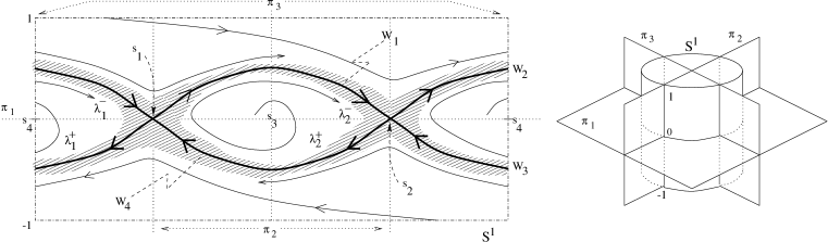
Figure 2: A sketch of the flow example of Bowen with symmetries

The following example shows how the global notion of stochastically stable systems is flexible enough to encompass systems for which time averages are not defined for Lebesgue almost every point.

Example 2:

The flow $(\phi_{t})_{t\geq 0}$ sketched on the left hand side of figure 2 is attributed to Bowen (cf. [21]) and is well known for showing that Birkhoff averages may not exist almost everywhere. In this system time averages exist only for the sources $s_{3},s_{4}$ and for the set of separatrixes and saddle equilibria $W=W_{1}\cup W_{2}\cup W_{3}\cup W_{4}\cup\{s_{1},s_{2}\}.$ Moreover the orbit $(\phi_{t}(x))_{t\geq 0}$ of each $x$ not in $W$ and different from $s_{3},s_{4}$ tends to $W$ as $t\to+\infty$.

Letting $f=\phi_{1}$ denote the time $1$ map of the flow, we see that $W$ is a compact $f$-invariant set and $W=\cap_{n\geq 0}f^{n}(U)$ for all sufficiently small neighborhoods $U$ of $W$. Hence $W$ lacks only transitiveness to become an attractor according to definition 2.1. However, defining $F:(S^{1}\times[-1,1])\times{{\mathbb{R}}}^{2}\longrightarrow S^{1}\times[-1,1]$ by

$$(x,y,(v_{1},v_{2}))\mapsto(x+v_{1}\bmod 1,y+v_{2})$$

where we identify $S^{1}$ with ${\mathbb{R}}/{\mathbb{Z}}$, and letting $B_{\epsilon}=\{(v_{1},v_{2})\in{{\mathbb{R}}}^{2}:v_{1}^{2}+v_{2}^{2}\leq\epsilon^{2}\}$ for small enough $\epsilon>0$, we have that the family $F$ is a physical random perturbation of $f$. In addition, as shown in [3, Prop. 10.1], there is a unique physical probability measure $\mu^{\epsilon}$ for the perturbed system whose support ${\rm supp\,}(\mu^{\epsilon})$ is a neighborhood of $W$, sketched in Figure 2 as a shaded region. This neighborhood is small for small $\epsilon>0$, satisfying all items of Proposition 2.1, although $W$ is not a transitive set.

The reason for this is that $W$ is chain-transitive or transitive with respect to pseudo-orbits. Indeed for all $\delta>0$ and every pair $x,y\in W$ there is a $\delta$-pseudo-orbit $(z_{k})_{k=0}^{n}$, for some $n\in{\mathbb{N}}$, such that $z_{0}=x$ and $z_{n}=y$, i.e., every pair of points of $W$ can be joined by some $\delta$-pseudo-orbit. Since random orbits are $\delta$-pseudo-orbits for some $\delta>0$, it is easily checked that the arguments of Proposition 2.1 can be repeated in this setting.

Finally we observe, on the one hand, that every weak^∗ accumulation point $\mu$ of $(\mu^{\epsilon})_{\epsilon>0}$, when $\epsilon\to 0$, is a $f$-invariant probability measure and, on the other hand, that $\mu$ must be a convex linear combination $\lambda\delta_{s_{1}}+(1-\lambda)\delta_{s_{2}}$, $0\leq\lambda\leq 1$, of the Dirac measures on the saddle fixed points. In fact every $f$-invariant probability measure must be a convex linear combination of $\delta_{s_{1}},\delta_{s_{2}},\delta_{s_{3}},\delta_{s_{4}}$ and ${\rm supp\,}(\mu)\subset{\rm supp\,}(\mu^{\epsilon})$ for all small $\epsilon>0$.

This means that $\delta_{s_{1}},\delta_{s_{2}}$ are stochastically stable! Indeed $C=\{\lambda\delta_{s_{1}}+(1-\lambda)\delta_{s_{2}}:0\leq\lambda\leq 1\}$ is a closed subset of $\mathcal{P}(M)$, the compact metrizable space of all probability measures on $M=S^{1}\times[-1,1]$ with the weak^∗ topology, and $(\mu^{\epsilon})_{\epsilon>0}$ is a family whose accumulation points all lie in $C$. Hence by compactness of $C$ and because the weak^∗ topology on $\mathcal{P}(M)$ is a metrizable one

$$\mu^{\epsilon}\longrightarrow\mbox{ convex hull }\{\delta_{s_{1}},\delta_{s_{2}}\}\qquad\mbox{when }\epsilon\to 0,$$

meaning that for all continuous $\varphi:M\to{\mathbb{R}}$ and for small enough $\epsilon>0$

$$\int\varphi\,d\mu^{\epsilon}\qquad\mbox{is close to}\qquad\Big{\{}\lambda\varphi(s_{1})+(1-\lambda)\varphi(s_{2}):0\leq\lambda\leq 1\Big{\}}.$$

3 Behavior of randomly perturbed orbits

We explain here the main ingredients involved in the proof of Theorems 1 and 2 recalling the main lemmas used in the proof of a general result in [3]. This result is stated below and guarantees the existence of a finite number of physical measures for general physical random perturbations. In subsection 3.2 we present a proof of proposition 2.1

Theorem 3.1

Under a physical random perturbation of fixed level $\epsilon>0$ of some diffeomorphism $f:M\longrightarrow M$, there are a finite number $\mu_{1},\ldots,\mu_{l}$ of physical probability measures in $M$ such that

1. ${\rm supp\,}\mu_{i}\cap{\rm supp\,}\mu_{j}=\emptyset$, $1\leq i<j\leq l$;

2. $\mu_{i}\ll m$ and ${\rm supp\,}(\mu_{i})$ contains a ball of radius $\xi=\xi(\epsilon)>0$, $i=1,\ldots,l$;

3. for every $x\in M$ there are open sets $V_{1}=V_{1}(x),\ldots,V_{l}=V_{l}(x)\subset\Delta_{\epsilon}$ such that

   1. $V_{i}\cap V_{j}=\emptyset$, $1\leq i<j\leq l$;

   2. $\nu_{\epsilon}^{\infty}(\Delta_{\epsilon}\setminus(V_{1}\cup\ldots\cup V_{l}))=0$;

   3. for every $1\leq i\leq l$ and all $\underline{t}\in V_{i}$ we have for every continuous $\varphi:M\longrightarrow{\mathbb{R}}$

      $$\frac{1}{n}\sum_{j=0}^{n-1}\varphi(f^{j}(x,\underline{t}))\longrightarrow\int\varphi\,d\mu_{i}\;\;\mbox{when}\;\;n\to\infty;$$ (10)

   4. $x\in{\rm supp\,}\mu_{i}\Longrightarrow V_{i}(x)=\Delta_{\epsilon}$, $\nu_{\epsilon}^{\infty}$-mod $0$, for $i=1,\ldots,l$;

   5. the $V_{i}(x)$ depend continuously on $x$ with respect to the metric $d_{\epsilon}(A,B)=\nu_{\epsilon}^{\infty}(A{\bigtriangleup}B)$, $A$, $B$ measurable subsets of $\Delta_{\epsilon}$.

Moreover every completely forward invariant nonempty set $C$ ($f_{t}(C)\subset C$ for all $t\in B_{\epsilon}$) contains ${\rm supp\,}\mu_{i}$ for some $i\in\{1,\ldots,l\}$ and ${\cal M}_{i}={\rm supp\,}\mu_{i}$ is a trapping region with respect to $f^{K}\equiv f_{0}^{K}$, i.e. $f_{t}^{K}({\cal M}_{i})\subset{\rm int\,}({\cal M}_{i})$ for all $i=1,\ldots,l$ (where $K=K(\epsilon)$ is given by condition II on $F$).

Proof:

See [3].    $\sqcup\!\!\!\!\sqcap$

In what follows we state the main lemmas used to prove Theorem 3.1 in [3].

3.1 Decomposing invariant probability measures

We assume that a diffeomorphism $f$ and a random perturbation $F$ of $f$ with fixed noise level $\epsilon>0$ are given. We set $S_{\epsilon}:M\times\Delta_{\epsilon}\to M\times\Delta_{\epsilon}$ to be the skew-product map $(x,\underline{t})\mapsto(f_{t_{1}}(x),\sigma\underline{t})$ where $\sigma$ is the usual left shift on sequences $\underline{t}=(t_{1},t_{2},\ldots)$.

Proposition 3.2

Let $D$ be a completely forward invariant subset of $M$ ($D=M$ is allowed). Given any $x\in D$ every $\mbox{weak}^{*}$ accumulation point $\mu$ of the sequence

$$\left(k^{-1}\sum_{j=0}^{k-1}f^{j}(x,\nu_{\epsilon}^{\infty})\right)_{k=1}^{\infty}$$ (11)

is a probability measure such that $\mu\times\nu_{\epsilon}^{\infty}$ is $S_{\epsilon}$-invariant and ${\cal M}={\rm supp\,}\mu$ is completely forward invariant, a trapping region for $f^{K}\equiv f^{K}_{0}$ and ${\cal M}\subset D$.

Proof:

V. [3, sects. 6, 7]. The $S_{\epsilon}$-invariance is trivial by construction of $\mu$ and definition of $S_{\epsilon}$. The complete forward invariance of ${\cal M}$ is an easy consequence of the form of $S_{\epsilon}$. If we take $K$ given by the property II of a physical random perturbation, that is $f^{K}(x,\Delta_{\epsilon})\supset B(f^{K}(x),\xi)$ for all $x\in D$, then we easily see that ${\cal M}$ is a trapping region for $f^{K}$.    $\sqcup\!\!\!\!\sqcap$

Definition 3.1

Given a probability measure $\mu$ such that $\mu\times\nu_{\epsilon}^{\infty}$ is $S_{\epsilon}$-invariant, we say that the set $B(\mu)=\left\{x\in M:k^{-1}\sum_{j=0}^{k-1}\delta_{f^{j}(x,\underline{t})}\stackrel{{\scriptstyle w^{*}}}{{\longrightarrow}}\mu\;\;\mbox{when}\;\;k\to\infty\;\;\mbox{for}\;\;\nu_{\epsilon}^{\infty}\mbox{a.e.}\;\underline{t}\in B_{\epsilon}\right\}$ is the basin of $\mu$.

Proposition 3.3

There are a finite number $\mu_{1},\ldots,\mu_{l}$ of probability measures in $M$ such that for all $1\leq i,j\leq l$

1. $\mu_{i}\times\nu_{\epsilon}^{\infty}$ is $S_{\epsilon}$-ergodic, ${\rm supp\,}\mu_{i}\cap{\rm supp\,}\mu_{j}=\emptyset$ and $\mu_{i}(\partial{\rm supp\,}\mu_{i})=0$;

2. $B(\mu_{i})\supset{\rm supp\,}\mu_{i}$;

3. for every probability measure $\mu$ such that $\mu\times\nu_{\epsilon}^{\infty}$ is $S_{\epsilon}$-invariant there are $\alpha_{1},\ldots,\alpha_{l}\geq 0$ with $\alpha_{1}+\ldots+\alpha_{l}=1$ such that $\mu=\alpha_{1}\mu_{1}+\ldots+\alpha_{l}\mu_{l}$.

Proof:

See [3, Sect.8].    $\sqcup\!\!\!\!\sqcap$

Remark 3.1

We observe that item 2 above corresponds to item 3d of Theorem 3.1.

The coefficients of item 3 of last proposition have a natural meaning.

Lemma 3.4

Let $\mu(x)$ be a $\mbox{weak}^{*}$ accumulation point of the sequence (11). Then

$$\alpha_{i}=\alpha^{\epsilon}_{i}(x)=\nu_{\epsilon}^{\infty}\{\underline{t}\in\Delta_{\epsilon}:\exists k\geq 1\;\;\mbox{such that}\;\;f^{k}(x,\underline{t})\in{\rm supp\,}\mu_{i}\},\;i=1,\ldots,l.$$

Consequently because $\alpha^{\epsilon}_{i}(x)$ depends only on $x$, we see that there is a single $\mbox{weak}^{*}$ accumulation point for the sequence (11) and thus we conclude that $\mu^{\epsilon}(x)$ is the weak^∗ limit of the sequence (11) when $k\to\infty$.

Proof:

We have $\mu(x)={\rm w^{*}}-\lim_{j\to\infty}k_{j}^{-1}\sum_{j=0}^{k_{j}-1}f^{j}(x,\nu_{\epsilon}^{\infty})$ for some sequence $k_{1}<k_{2}<\ldots$ of integers. According to proposition 3.3 there are $\alpha_{1},\ldots,\alpha_{l}\geq 0$ with $\alpha_{1}+\ldots+\alpha_{l}=1$ and $\mu_{1},\ldots,\mu_{l}$ satisfying $\mu(x)=\alpha_{1}\mu_{1}+\ldots+\alpha_{l}\mu_{l}$. Since the $\mu_{1},\ldots,\mu_{l}$ have pairwise disjoint compact supports, it must be that $\mu_{i}({\rm supp\,}\mu_{i})=\delta_{ij}$ (Kronecker delta), $i,j=1,\ldots,l$. Therefore $\mu(x)({\rm supp\,}\mu_{i})=\alpha_{i}$, $1\leq i\leq l$.

The construction of $\mu(x)$ tells us then that, because $\mu_{i}(\partial{\rm supp\,}\mu_{i})=0$,

$$\alpha_{i}=\alpha_{i}(x)=\lim_{h\to\infty}\frac{1}{k_{h}}\sum_{j=0}^{k_{h}-1}\nu_{\epsilon}^{\infty}(V_{i}^{j}(x))\;\;\mbox{where}\;\;V_{i}^{j}(x)=\{\underline{t}\in\Delta_{\epsilon}:f^{j}(x,\underline{t})\in{\rm supp\,}\mu_{i}\}.$$

Observing that $V_{i}^{j}(x)\subset V_{i}^{j+1}(x)$ by the invariance of ${\rm supp\,}\mu_{i}$, $i=1,\ldots,l;j\geq 1$, we see that defining $V_{i}(x)=\{\underline{t}\in\Delta_{\epsilon}:\exists k\geq 1\;\mbox{s.t.}\;f^{k}(x,\underline{t})\in{\rm supp\,}\mu_{i}\}=\cup_{j\geq 1}V_{i}^{j}(x)$ we arrive at $\nu_{\epsilon}^{\infty}(V_{i})=\lim_{j\to\infty}\nu_{\epsilon}^{\infty}(V^{j}_{i}(x))=\lim_{k\to\infty}k^{-1}\sum_{j=0}^{k-1}\nu_{\epsilon}^{\infty}(V_{i}^{j}(x))=\alpha_{i}(x)$.    $\sqcup\!\!\!\!\sqcap$

Finally, after these propositions, for any given $x\in M$ the unique probability $\mu(x)$ decomposes in a unique way $\alpha_{1}\mu_{1}+\ldots+\alpha_{l}\mu_{l}$ and $\Delta_{\epsilon}$ has a $\nu_{\epsilon}^{\infty}$ mod $0$ partition $V_{1},\ldots,V_{l}$ since, clearly, the $V_{1}=V_{1}(x),\ldots,V_{l}=V_{l}(x)$ are pairwise disjoint by definition and their total $\nu_{\epsilon}^{\infty}$ measure is $\alpha_{1}+\cdots+\alpha_{l}=1$.

3.2 Localizing physical probability measures

Now we are able to prove Proposition 2.1.

Proof of 2.1:

We suppose that $\Lambda$ is an attractor, that for a given open set $U$ we have $\Lambda=\cap_{k\geq 0}f^{k}(U)$ and $f(\overline{U})\subset U$ and that $F$ is a physical random perturbation of $f$. The parameterized family $F$ given by the map $F:M\times B_{1}(0)\longrightarrow M$ is such that, by continuity

$${\rm diam\,}(f(x,\Delta_{\epsilon}))=\sup\big{\{}{\rm dist\,}\left(f_{t}(x),f_{s}(x)\right),t,s\in B_{\epsilon}\big{\}}\longrightarrow 0\;\;\mbox{when}\;\;\epsilon\longrightarrow 0^{+}.$$ (12)

Therefore for sufficiently small $\delta_{0}>0$ the open set $U$ is a trapping region with respect to $f_{t}$ for all $\epsilon\in]0,\delta_{0}[$ and every $t\in B_{\epsilon}$. In particular this means that $U$ is a completely forward invariant set and then there is some physical probability $\mu^{\epsilon}$ with ${\rm supp\,}\mu^{\epsilon}\subset U$ by Theorem 3.1.

It is easy to see that ${\cal M}^{\epsilon}={\rm supp\,}\mu^{\epsilon}$ is a compact forward $f_{t}$-invariant set $f_{t}({\cal M}^{\epsilon})\subset{\cal M}^{\epsilon}$ for each $t\in B_{\epsilon}$ and $\epsilon\in]0,\delta_{0}[$. Indeed $({\rm supp\,}\mu^{\epsilon})\times\Delta_{\epsilon}={\rm supp\,}(\mu^{\epsilon}\times\nu_{\epsilon}^{\infty})$ is $S_{\epsilon}$-invariant and the definition of $S_{\epsilon}$ gives the invariance of ${\cal M}^{\epsilon}$. In particular ${\cal M}^{\epsilon}$ is forward $f$-invariant ($f\equiv f_{0}$). On the one hand $\Lambda\supset\cap_{k\geq 0}f^{k}({\cal M}^{\epsilon})$ since $\Lambda$ is the maximal forward $f$-invariant set in $U\supset{\cal M}^{\epsilon}$. On the other hand ${\cal M}^{\epsilon}$ is a $f_{t}^{K}$-trapping region (by Theorem 3.1) and so $\cap_{k\geq 0}f^{k}({\cal M}^{\epsilon})\subset{\rm int\,}({\cal M}^{\epsilon})$. Thus $\Lambda\cap{\rm int\,}({\cal M}^{\epsilon})\neq\emptyset$. Because $\Lambda$ is $f$-transitive and ${\cal M}^{\epsilon}$ is forward $f$-invariant, it must be that $\Lambda\subset{\rm int\,}({\cal M}^{\epsilon})$.

Observing that this holds for every physical probability measure $\mu^{\epsilon}$ with ${\rm supp\,}\mu^{\epsilon}\subset U$, and that for every random perturbation of fixed level $\epsilon$ the supports of the physical probability measures are pairwise disjoint by item 1 of Theorem 3.1, we deduce that there is a unique physical probability measure $\mu^{\epsilon}$ inside $U$. This provides items $(a)$ and $(b)$ and the uniqueness part of Proposition 2.1. In addition the orbital averages of any $x\in U$ must satisfy item $(c)$, since the random orbits cannot leave $U$ and their time averages exist and are given by a physical probability measure (Theorem 3.1 again). It must be $\mu^{\epsilon}$ by the previous uniqueness arguments.

To get $(d)$ we first note that $\Lambda\subset{\rm supp\,}(\mu^{\epsilon})$ for all small $\epsilon>0$. Now we just need to show that for any given neighborhood $W$ of $\Lambda$ we may find $\delta_{0}$ such that ${\rm supp\,}(\mu^{\epsilon})\subset W$ for every $\epsilon\in]0,\delta_{0}[$. It is easy to see that the set $U_{l}=\cap_{k=0}^{l}f^{k}(U)$ satisfies ${\rm dist\,}(U\setminus U_{l},\Lambda)\longrightarrow 0\;\;\mbox{when}\;\;l\longrightarrow\infty$, i.e. $W\supset U_{l}$ for big enough $l$, and $\Lambda\subset f(\overline{U}_{l})\subset U_{l}$ for all $l\geq 1$. Hence (12) ensures that for given $l\geq 1$ there is $\delta_{0}>0$ such that $f_{t}(\overline{U}_{l})\subset U_{l}$ for all $t\in B_{\epsilon}$ and $\epsilon\in]0,\delta_{0}[$. Thus ${\rm supp\,}\mu_{\epsilon}\subset U_{l}$ for all $\epsilon\in]0,\delta_{0}[$ with $\delta_{0}(l)\longrightarrow 0$ as $l\longrightarrow\infty$. This shows that ${\rm supp\,}(\mu^{\epsilon})\to\Lambda$ in the Hausdorff topology when $\epsilon\to 0$.    $\sqcup\!\!\!\!\sqcap$

4 Stochastic stability

Here we assume that $f$ is a diffeomorphism satisfying conditions $\underline{A}$ and $\underline{B}$ of Theorem 1.

Lemma 4.1

If $\mu_{i}^{\epsilon}$ is the physical probability measure provided by Proposition 2.1 for all small enough $\epsilon>0$, then $m[W^{s}(\Lambda_{i})\setminus B(\mu_{i}^{\epsilon})]\longrightarrow 0$ when $\epsilon\to 0^{+}$ for $i\in\{1,\ldots,N\}$.

Proof:

We fix $i\in\{1,\ldots,N\}$ and observe that because $\Lambda=\Lambda_{i}$ is an attractor there is a trapping region $U$ such that $\Lambda=\cap_{n\geq 1}f^{n}(\overline{U})$. By definition of basin of attraction $W^{s}(\Lambda)=\cup_{j=0}^{\infty}f^{-j}(\overline{U})$ and since $U$ is a trapping region $f^{-j-1}(\overline{U})\supset f^{-j}(\overline{U})$ for all $j\geq 0$. By Proposition 2.1 there is $\delta_{0}>0$ such that for every $\epsilon\in]0,\delta_{0}[$ it exists a physical measure $\mu^{\epsilon}=\mu^{\epsilon}_{i}$ satisfying ${\rm supp\,}(\mu^{\epsilon})\subset U$ and $B(\mu^{\epsilon})\supset U$. We have to show that for all $j\geq 1$ there is $\delta_{1}\in]0,\delta_{0}[$ such that for every $\epsilon\in]0,\delta_{1}[$ it holds that $B(\mu^{\epsilon})\supset f^{-j}(\overline{U})$.

Let us fix an arbitrary integer $j\geq 1$. Then for all $x\in f^{-j}(\overline{U})$ we know that, because $U$ is a trapping region and by the continuity of the map $f^{j+1}(x,\cdot):\Delta_{\delta_{0}}\to M$, there is $\delta_{1}\in]0,\delta_{0}[$ such that $f^{j+1}(x,\Delta_{\epsilon})\subset U$ for all $\epsilon\in]0,\delta_{1}[$. By compactness of $f^{-j}(\overline{U})$ ($f$ is a diffeomorphism) the value $\delta_{1}$ may be taken to depend on $j$ alone. It is easy to see that if $f^{j+1}(x,\underline{t})\in B(\mu^{\epsilon})$ for fixed $j\geq 1$ and for $\nu_{\epsilon}^{\infty}$ almost all $\underline{t}\in\Delta_{\epsilon}$, then $x\in B(\mu^{\epsilon})$ also. We conclude that $B(\mu^{\epsilon})\supset f^{-j-1}(\overline{U})\supset f^{-j}(\overline{U})$ for all $\epsilon\in]0,\delta_{1}[$.    $\sqcup\!\!\!\!\sqcap$

Remark 4.1

The proof of this lemma shows that $B(\mu_{i}^{\epsilon})$ is a nondecreasing function of $\epsilon$.

Now for $i\in\{1,\ldots,N\}$ we define the thresholds

$$\epsilon_{i}=\sup\left\{\delta\in]0,1[:\forall\epsilon\in]0,\delta[\;\;\exists!\mu_{i}^{\epsilon}\;\;\mbox{such that}\;\Lambda_{i}\subset{\rm supp\,}(\mu_{i}^{\epsilon})\subset{\rm supp\,}(\mu_{i}^{\delta})\right\}$$ (13)

(the set is nonempty by Proposition 2.1). We observe that when the number $N$ of attractors is infinite, it must be that $\inf_{i}\{\epsilon_{i}\}=0$ for otherwise we would have an infinite number of physical measures $(\mu_{i}^{\epsilon})_{i\geq 1}$ for $\epsilon\in]0,\inf_{i}\{\epsilon_{i}\}[$ such that $({\rm supp\,}(\mu_{i}^{\epsilon}))_{i\geq 1}$ are pairwise disjoint and each contains a ball of radius $\xi=\xi(\epsilon)>0$ (by Theorem 3.1). This is impossible in a compact space. Now we may reindex the attractors in such a way that $\epsilon_{1}\geq\epsilon_{2}\geq\ldots$ holds. If we define $N(\delta)=\sup\{i\geq 1\;:\;\epsilon_{i}\geq\delta,i\geq 1\}$ and ${\cal V}_{\delta}=\cup_{i=1}^{N(\delta)}B(\mu_{i}^{\delta})$, then $m({\cal V}_{\delta})\to 1$ when $\delta\to 0$, because Condition $\underline{A}$ of Theorem 1 and Lemma 4.1 easily imply that $\sum_{j=1}^{N(\epsilon)}m\big{(}B(\mu_{i}^{\epsilon})\big{)}\to 1$ when $\epsilon\to 0$.

It is now easy to prove item 1 of Theorem 1 because the weak^∗ limit of the sequence (11) is the same as the limit in the definition (4) of mean sojourn times. Indeed, according to Lemma 4.1 and Remark 4.1, for $m$ almost every $x\in M$ there is $\epsilon_{x}>0$ such that if $\epsilon\in]0,\epsilon_{x}[$, then $x\in B(\mu_{i}^{\epsilon})$ for some $i=i(x)\in\{1,\ldots,N\}$. Hence $\mu^{\epsilon}(x)=\mu_{i}^{\epsilon}$ and Condition $\underline{B}$ says that $\mu_{i}^{\epsilon}\to\mu_{i}$ when $\epsilon\to 0$ in the weak^∗ topology.

For the proof of item 2 of Theorem 1 we observe that the probability measure $\mu^{\epsilon}$ satisfies for all continuous $\varphi:M\to{\mathbb{R}}$

$$\mu^{\epsilon}(\varphi)=\lim_{n\to+\infty}\frac{1}{n}\sum_{j=0}^{n-1}\int\!\!\!\int\varphi(f^{j}(x,\underline{t}))\,d\nu_{\epsilon}^{\infty}(\underline{t})dm(x)$$ (14)

if the limit exists for fixed $\epsilon>0$. On the one hand, for all $x\in M$ we know that $\lim_{n\to\infty}n^{-1}\sum_{j=0}^{n-1}\varphi(f^{j}(x,\underline{t}))\,d\nu_{\epsilon}^{\infty}(\underline{t})=\alpha_{1}^{\epsilon}(x)\mu_{1}^{\epsilon}(\varphi)+\ldots+\alpha_{l}^{\epsilon}(x)\mu_{l}^{\epsilon}(\varphi)$ by Proposition 3.2 and item 3 of Proposition 3.3. It is clear that $\sup_{x}\big{|}n^{-1}\sum_{j=0}^{n-1}\varphi(f^{j}(x,\underline{t}))\,d\nu_{\epsilon}^{\infty}(\underline{t})\big{|}=\|\varphi\|_{0}$ for all $n\geq 1$ and (14) equals $\int[\lim_{n\to\infty}n^{-1}\sum_{j=0}^{n-1}\varphi(f^{j}(x,\underline{t}))\,d\nu_{\epsilon}^{\infty}(\underline{t})]dm(x)$ by Lebesgue’s Dominated Convergence Theorem. So (14) also equals $\beta_{1}^{\epsilon}\mu_{1}^{\epsilon}(\varphi)+\ldots+\beta_{l}^{\epsilon}\mu_{l}^{\epsilon}(\varphi)$ if we define $\beta_{i}^{\epsilon}=\int\alpha_{i}^{\epsilon}\,dm$, $i=1,\ldots,l=l(\epsilon)$ — note that $\beta_{i}^{\epsilon}$ is well defined by item 3e of Theorem 3.1. This proves (7).

On the other hand (8) is easy when $N$ is finite since $\mu^{\epsilon}=\beta_{1}^{\epsilon}\mu_{1}^{\epsilon}+\cdots+\beta_{N}^{\epsilon}\mu_{N}^{\epsilon}$ for $\epsilon\in]0,\inf\{\epsilon_{1},\ldots,\epsilon_{N}\}[$ and Condition $\underline{B}$ suffices to get the convergence if we show that $\lim_{\epsilon\to 0}\beta_{i}^{\epsilon}=m(W^{s}(\Lambda_{i}))$, $i=1,\ldots,N$. But in fact $\alpha_{i}^{\epsilon}(x)=\nu_{\epsilon}^{\infty}(V_{i}(x))$ by the proof of Lemma 3.4 and $\alpha_{i}^{\epsilon}(x)=1$ if $x\in B(\mu_{i}^{\epsilon})$ by item 3 of Theorem 3.1. So $\beta_{i}^{\epsilon}\geq m(B(\mu_{i}^{\epsilon}))$ and then $\liminf_{\epsilon\to 0}\beta_{i}^{\epsilon}\geq m(W^{s}(\Lambda_{i}))$ by Lemma 4.1. Since $m$ is a probability measure Condition $\underline{A}$ together with Lemma 4.1 imply that $\limsup_{\epsilon\to 0}\beta_{i}^{\epsilon}\leq m(W^{s}(\Lambda_{i}))$.

Now we assume that $N$ is infinite. It is obvious that $l(\epsilon)\geq N(\epsilon)\to+\infty$ when $\epsilon\to 0$. Let $\beta_{i}=m(W^{s}(\Lambda_{i}))$ for $i\geq 1$. Fixing a continuous map $\varphi:M\to{\mathbb{R}}$ we want to bound $D(\varphi,\epsilon)=\big{|}\sum_{i=1}^{l(\epsilon)}\beta_{i}^{\epsilon}\mu_{i}^{\epsilon}(\varphi)-\sum_{i\geq 1}\beta_{i}\mu_{i}(\varphi)\big{|}$ by a quantity tending to zero when $\epsilon\to 0$.

Let us fix $\delta>0$. Then it exists $I\geq 1$ such that $\sum_{i\geq I}\beta_{i}<\delta$ by Condition $\underline{A}$ and

$${\textstyle D(\varphi,\epsilon)} \leq {\textstyle\big{|}\sum_{i=1}^{I}\beta_{i}^{\epsilon}\mu_{i}^{\epsilon}(\varphi)-\sum_{i=1}^{I}\beta_{i}\mu_{i}(\varphi)\big{|}+\big{|}\sum_{i=I+1}^{l(\epsilon)}\beta_{i}^{\epsilon}\mu_{i}^{\epsilon}(\varphi)-\sum_{i=I+1}^{l(\epsilon)}\beta_{i}\mu^{\epsilon}_{i}(\varphi)\big{|}}$$

$${\textstyle+\big{|}\sum_{i=I+1}^{l(\epsilon)}\beta_{i}\mu_{i}^{\epsilon}(\varphi)-\sum_{i>I}\beta_{i}\mu_{i}(\varphi)\big{|}=D_{1}+D_{2}+D_{3}.}$$

for $\epsilon\in]0,\epsilon(I)[$ where $\epsilon(I)=\sup\{\epsilon\in]0,1[:l(\epsilon)>I\}$. By previous arguments $D_{1}\to 0$ when $\epsilon\to 0$. It is easy to see that $D_{3}\leq(\sum_{i>I}\beta_{i})(\|\varphi\|_{0}+\|\varphi\|_{0})\leq 2\delta\|\varphi\|_{0}$. If we take $\epsilon_{0}\in]0,\epsilon(I)[$ such that $|\beta_{i}^{\epsilon}-\beta_{i}|<\delta/I$ for $\epsilon\in]0,\epsilon_{0}[$ and $i=1,\ldots,I$, then $\sum_{i=I+1}^{l(\epsilon)}\beta_{i}^{\epsilon}<2\delta$ because $\sum_{i=1}^{l(\epsilon)}=1$. Thus $D_{2}\leq\sum_{i=I+1}^{l(\epsilon)}(\beta_{i}^{\epsilon}+\beta_{i})|\mu_{i}^{\epsilon}(\varphi)|\leq 3\delta\|\varphi\|_{0}$ for $\epsilon\in]0,\epsilon_{0}[$. This shows that $D(\varphi,\epsilon)\to 0$ when $\epsilon\to 0$ for any fixed continuous map $\varphi:M\to{\mathbb{R}}$ and concludes the proof of Theorem 1.

4.1 Convergence to finitely many measures

To prove Theorem 2 we now assume that $f$ satisfies Conditions $\underline{B}$ and $\underline{C}$ for a finite family $\Lambda_{1},\ldots,\Lambda_{N}$, of attractors. We observe that although Lemma 4.1 no longer holds, we may still define the thresholds $\epsilon_{1}\geq\ldots\geq\epsilon_{N}>0$ as before for a physical random perturbation $F$ of $f$ by Proposition 2.1. For $\epsilon\in]0,\epsilon_{N}[$ and $x\in M$ there are $l=l(\epsilon)\geq N$ physical probability measures such that $\mu^{\epsilon}(x)=\alpha_{1}^{\epsilon}(x)\mu_{1}^{\epsilon}+\ldots+\alpha_{l}^{\epsilon}(x)\mu_{l}^{\epsilon}$ where $\alpha_{1}^{\epsilon}(x),\ldots,\alpha_{l}^{\epsilon}(x)\geq 0$ and $\sum_{i=1}^{l(\epsilon)}\alpha_{i}^{\epsilon}(x)=1$, by Propositions 3.2 and 3.3.

If we show that $l(\epsilon)=N$ for $\epsilon\in]0,\epsilon_{N}[$, then Condition $\underline{B}$ and Proposition 2.1 together imply that $\mu_{i}^{\epsilon}\stackrel{{\scriptstyle w^{*}}}{{\longrightarrow}}\mu_{i}$ when $\epsilon\to 0$ for $i=1,\ldots,N$ and so we would get (9).

Arguing by contradiction, we suppose that $l(\epsilon)>N$ for $\epsilon\in]0,\epsilon_{N}[$. Then there is a physical measure $\mu_{N+1}^{\epsilon}$ and ${\rm supp\,}(\mu_{N+1})$ is a trapping region for $f^{K}$, where $K=K(\epsilon)$ from Condition II on $F$, by Theorem 3.1. According to Proposition 2.9 of [19], any trapping region for $f^{K}$ contains a trapping region for $f$. Then Condition $\underline{C}$ would ensure that ${\rm supp\,}(\mu_{N+1}^{\epsilon})$ contains $\Lambda_{i}$ for $i\in\{1,\ldots,N\}$. But we note that ${\rm supp\,}(\mu_{i}^{\epsilon})\supset\Lambda_{i}$ for $i=1,\ldots,N$, by Proposition 2.1 since $\epsilon<\epsilon_{N}$ and also remark that $({\rm supp\,}(\mu_{i}^{\epsilon}))_{i=1,\ldots,l(\epsilon)}$ are pairwise disjoint by Theorem 3.1. We have arrived at a contradiction. Hence we have showed that $l(\epsilon)=N$ for all $\epsilon\in]0,\epsilon_{N}[$ and thus proved Theorem 2.

Vítor Araújo

Centro de Matemática da Universidade do Porto

Rua do Campo Alegre 687, 4169-007 Porto, Portugal.

and

Instituto de Matemática, Universidade Federal do Rio de Janeiro,

C. P. 68.530, 21.945-970 Rio de Janeiro, RJ-Brazil

Email: vitor.araujo@im.ufrj.br and vdaraujo@fc.up.pt

References

- [1] Alves, J.; Araújo, V.; Random perturbations of nonuniformly expanding maps, preprint CMUP (2000).
- [2] Alves, J.; Bonatti, C.; Viana, M., SRB measures for partially hyperbolic systems whose central direction is mostly expanding, Invent. Math. 140 (2000) 351-398.
- [3] Araújo, V., Attractors and Time Averages for Random Maps, Ann. de l’Inst. H. Poincaré – Anal. Non Linéaire 17, 3 (2000) 307-369.
- [4] Benedicks, M.; Viana, M.; Random Perturbations and Statistical Properties of some Hénon-like maps, in preparation.
- [5] Bonatti, C; Díaz, L.J.; Connections heterocliniques et genericité d’une infinité de puis ou de sources, Ann. Sci. Ec. Norm. Super. IV, Ser. 32, No. 1 (1999) 135-150.
- [6] Bonatti, C.; Viana, M., SRB measures for partially hyperbolic systems whose central direction in mostly contracting, to appear in Israel Journal Math.
- [7] Bowen, R., Equilibrium States and the Ergodic Theory of Anosov Diffeomorphisms, Lect. Notes in Math. 470, Berlin: Springer-Verlag, 1975.
- [8] Bowen, R.; Ruelle, D.; The Ergodic Theory of Axiom A flows, Invent. Math. 29 (1975) 181-202.
- [9] Colli, E., Infinitely many coexisting strange attractors, Ann. de l’Inst. H. Poincaré – Anal. Non Linéaire 15 no. 5 (1998) 539-579.
- [10] Kifer, Y., Ergodic Theory of Random Perturbations, Basel: Birkhauser, 1998.
- [11] Kifer, Y., Random Perturbations of Dynamical Systems, Basel: Birkhauser, 1988.
- [12] Lorenz, E.N., Deterministic nonperiodic flow, J. Atmosph. Sci. 20 (1963) 130-141.
- [13] Newhouse, S., Non-density of Axiom A(a) on , Proc. A.M.S. Symp. Pure Math. 14 (1970) 191-202.
- [14] Newhouse, S., Diffeomorphisms with infinitely many sinks, Topology 13 (1974) 9-18.
- [15] Newhouse, S., The abundance of wild hyperbolic sets and nonsmooth stable sets for diffeomorphisms, Publ. Math. I.H.E.S. no. 50 (1979) 101-151.
- [16] Palis, J., Takens, F., Hyperbolicity and Sensitive Chaotic Dynamics at Homoclinic Bifurcations, Cambridge Studies in Adv. Math., no. 35, 1993.
- [17] Pumariño, A.; Rodriguez, J. A.; Coexistence and Persistence of Strange Attractors, Lect. Notes in Math. no. 1658, Berlin: Springer-Verlag, 1997.
- [18] Ruelle, D., A measure associated with Axiom A attractors, Amer. J. Math. 98 (1976) 619-654.
- [19] Shub, M., Global Stability of Dynamical Systems, New York-Springer Verlag, 1987.
- [20] Sinai, Ya., Gibbs measures in Ergodic Theory, Russian Math. Surveys 27 (1972) 21-69.
- [21] Takens, F., Heteroclinic attractors: time averages and moduli of topological conjugacy, Bul. Soc. Bras. Mat., Vol 25, no. 1 (1994) 107-120.
- [22] Viana, M, Multidimensional nonhyperbolic attractors, Publ. Math. IHES 85 (1997) 63-96.
- [23] Viana, M., Stochastic Dynamics of Deterministic Systems, Colóquio Brasileiro de Matemática, Rio de Janeiro: IMPA, 1997.
- [24] Viana, M., Dynamics: A Probabilistic and Geometric Perspective, Proceedings ICM 1998 – Documenta Mathematica.
- [25] Young, L.-S., Stochastic Stability of Hyperbolic Attractors, Erg. Th. & Dyn. Sys. 6 (1986) 311-319.