Cohomology of Categorical Self-Distributivity

Abstract

We define self-distributive structures in the categories of coalgebras and cocommutative coalgebras. We obtain examples from vector spaces whose bases are the elements of finite quandles, the direct sum of a Lie algebra with its ground field, and Hopf algebras. The self-distributive operations of these structures provide solutions of the Yang–Baxter equation, and, conversely, solutions of the Yang–Baxter equation can be used to construct self-distributive operations in certain categories.

Moreover, we present a cohomology theory that encompasses both Lie algebra and quandle cohomologies, is analogous to Hochschild cohomology, and can be used to study deformations of these self-distributive structures. All of the work here is informed via diagrammatic computations.

1 Introduction

In the past several decades, operations satisfying self-distributivity [$(a\triangleleft b)\triangleleft c=(a\triangleleft c)\triangleleft(b\triangleleft c)$] have secured an important role in knot theory. Such operations not only provide solutions of the Yang–Baxter equation and satisfy a law that is an algebraic distillation of the type (III) Reidemeister move, but they also capture one of the essential properties of group conjugation. Sets possessing such a binary operation are called shelves. Adding an axiom corresponding to the type (II) Reidemeister move amounts to the property that the set acts on itself (on the right) bijectively and thus gives the structure of a rack. Further introducing a condition corresponding to the type (I) Reidemeister move has the effect of making each element idempotent and gives the structure of a quandle. Keis, or involutory quandles, satisfy an extra involutory condition. Such structures were discussed as early as the 1940s [25].

The primordial example of a self-distributive operation comes from group conjugation: $x\triangleleft y=y^{-1}xy$. This operation satisfies the additional quandle axioms which are stated in the sequel. Quandle cohomology has been studied extensively in connection with applications to knots and knotted surfaces [10, 11]. Analogues of self-distributivity in a variety of categorical settings have been discussed as adjoint maps in Lie algebras  [12] and quantum group theories (see for example [20, 19]). In particular, the adjoint map $x\otimes y\mapsto S(y_{(1)})xy_{(2)}$ of Hopf algebras is a direct analogue of group conjugation. Thus, analogues of self-distributive operations are found in a variety of algebraic structures where cohomology theories are also defined.

In this paper, we study how quandles and racks and their cohomology theories are related to these other algebraic systems and their cohomology theories. Specifically, we treat self-distributive maps in a unified manner via a categorical technique called internalization  [13]. Then we develop a cohomology theory and provide explicit relations to rack and Lie algebra cohomology theories. Furthermore, this cohomology theory can be seen as a theory of obstructions to deformations of self-distributive structures.

The organization of this paper is as follows: Section 2 consists of a review of the fundamentals of quandle theory, internalization in a category, and the definition of a coalgebra. Section 3 contains a collection of examples that possess a self-distributive binary operation. In particular, a motivating example built from a Lie algebra is presented. In Section 4 we relate the ideas of self-distributivity to solutions of the Yang-Baxter equation, and demonstrate connections of these ideas to Hopf algebras. Section 5 contains a review of Hochschild cohomology from the diagrammatic point of view and in relation to deformations of algebras. These ideas are imitated in Section 6 where the most original and substantial ideas are presented. Herein a cohomology theory for shelves in the coalgebra category is defined in low dimensions. The theory is informed by the diagrammatic representation of the self-distributive operation, the comultiplication, their axioms, and their relationships. Section 7 contains the main results of the paper. Theorems 7.4 through 7.9 state that the cohomology theory is non-trivial, and that non-trivial quandle cocycles and Lie algebra cocycles give non-trivial shelf cocycles in dimension $2$ and $3$.

Acknowledgements

In addition to the National Science Foundation who supported this research financially, we also wish to thank our colleagues whom we engaged in a number of crucial discussions. The topology seminar at South Alabama listened to a series of talks as the work was being developed. Joerg Feldvoss gave two of us a wonderful lecture on deformation theory of algebras and helped provide a key example. John Baez was extremely helpful with some fundamentals of categorical constructions. We also thank N. Apostolakis, L.H. Kauffman, and D. Radford for valuable conversations.

2 Internalized Shelves

2.1 Review of Quandles

A quandle, $X$, is a set with a binary operation $(a,b)\mapsto a\triangleleft b$ such that

(I) For any $a\in X$, $a\triangleleft a=a$.

(II) For any $a,b\in X$, there is a unique $c\in X$ such that $a=c\triangleleft b$.

(III) For any $a,b,c\in X$, we have $(a\triangleleft b)\triangleleft c=(a\triangleleft c)\triangleleft(b\triangleleft c).$

A rack is a set with a binary operation that satisfies (II) and (III). Racks and quandles have been studied extensively in, for example, [6, 14, 16, 23].

The following are typical examples of quandles: A group $G$ with conjugation as the quandle operation: $a\triangleleft b=b^{-1}ab$, denoted by $X=$ Conj$(G)$, is a quandle. Any subset of $G$ that is closed under such conjugation is also a quandle. More generally if $G$ is a group, $H$ is a subgroup, and $s$ is an automorphism that fixes the elements of $H$ (i.e. $s(h)=h\ \forall h\in H$), then $G/H$ is a quandle with $\triangleleft$ defined by $Ha\triangleleft Hb=Hs(ab^{-1})b.$ Any $\Lambda(={\mathbb{Z}}[t,t^{-1}])$-module $M$ is a quandle with $a\triangleleft b=ta+(1-t)b$, for $a,b\in M$, and is called an Alexander quandle. Let $n$ be a positive integer, and for elements $i,j\in\{0,1,\ldots,n-1\}$, define $i\triangleleft j\equiv 2j-i\pmod{n}$. Then $\triangleleft$ defines a quandle structure called the dihedral quandle, $R_{n}$, that coincides with the set of reflections in the dihedral group with composition given by conjugation.

The third quandle axiom $(a\triangleleft b)\triangleleft c=(a\triangleleft c)\triangleleft(b\triangleleft c)$, which corresponds to the type (III) Reidemeister move, can be reformulated to make sense in a more general setting. In fact, we do not need the full-fledged structure of a quandle; we simply need a structure having a binary operation satisfying the self-distributive law. We call a set together with a binary operation satisfying the self-distributive axiom (III) a shelf.

We reformulate the self-distributive operation of a shelf as follows: Let $X$ be a shelf with the shelf operation denoted by a map $q:X\times X\rightarrow X$. Define $\Delta:X\rightarrow X\times X$ by $\Delta(x)=(x,x)$ for any $x\in X$, and $\tau:X\times X\rightarrow X\times X$ by a transposition $\tau(x,y)=(y,x)$ for $x,y\in X$. Then axiom (III) above can be written as:

$$q(q\times 1)=q(q\times q)(1\times\tau\times 1)(1\times 1\times\Delta):X^{3}\rightarrow X.$$

It is natural and useful to formulate this axiom for morphisms in certain categories. This approach was explored in [12] (see also [2]) and involves a technique known as internalization.

2.2 Internalization

All familiar mathematical concepts were defined in the category of sets, but most of these can live in other categories as well. This idea, known as internalization, is actually very familiar. For example, the notion of a group can be enhanced by looking at groups in categories other than ${\rm Set}$, the category of sets and functions between them. We have the notions of topological groups, which are groups in the category of topological spaces, Lie groups, groups in the category of smooth manifolds, and so on. Internalizing a concept consists of first expressing it completely in terms of commutative diagrams and then interpreting those diagrams in some sufficiently nice ambient category, $K$. In this paper, we consider the notion of a shelf in the categories of coalgebras and cocommutative coalgebras. Thus, we define the notion of an internalized shelf, or shelf in $K$. This concept is also known as a shelf object in $K$ or internal shelf.

Given two objects $X$ and $Y$ in an arbitrary category, we define their product to be any object $X\times Y$ equipped with morphisms $\pi_{1}:X\times Y\rightarrow X$ and $\pi_{2}:X\times Y\rightarrow Y$ called projections, such that the following universal property is satisfied: for any object $Z$ and morphisms $f:Z\rightarrow X$ and $g:Z\rightarrow Y,$ there is a unique morphism $h:Z\rightarrow X\times Y$ such that $f=\pi_{1}h$ and $g=\pi_{2}h$. Note that this product does not necessarily exist, nor is it unique. However, it is unique up to canonical isomorphism, which is why we refer to the product when it exists. We say a category has binary products when every pair of objects has a product. Trinary products $(X\times Y)\times Z$ and $X\times(Y\times Z)$ are defined similarly, are canonically isomorphic, and denoted by $X\times Y\times Z$ if the isomorphism is the identity. Inductively, $n$-ary products are defined. We say a category has finite products if it has $n$-ary products for all $n\geq 0$. Note that whenever $X$ is an object in some category for which the product $X\times X$ exists, there is a unique morphism called the diagonal $D:X\rightarrow X\times X$ such that $\pi_{1}D=1_{X}$ and $\pi_{2}D=1_{X}$. In the category of sets, this map is given by $D(x)=(x,x)$ for all $x\in X$. In a category with finite products, we also have a transposition morphism given by $\tau:X\times X\rightarrow X\times X$ by $\tau=(\pi_{2}\times\pi_{1})D_{X\times X}$.

Definition 2.1

Let $X$ be an object in a category $K$ with finite products. A map $q:X\times X\rightarrow X$ is a self-distributive map if the following diagram commutes:

where $\Delta:X\rightarrow X\times X$ is the diagonal morphism in $K$ and $\tau:X\times X\rightarrow X\times X$ is the transposition. We also say that a map $q$ satisfies the self-distributive law.

Definition 2.2

Let $K$ be a category with finite products. A shelf in $K$ is a pair $(X,q)$ such that $X$ is an object in $K$ and $q:X\times X\rightarrow X$ is a morphism in $K$ that satisfies the self-distributive law of Definition 2.1.

Example 2.3

A quandle $(X,q)$ is a shelf in the category of sets, with the cartesian products and the diagonal map $D:X\rightarrow X\times X$ defined by $D(x)=(x,x)$ for all $x\in X$. Thus the language of shelves and self-distributive maps in categories unifies all examples discussed in this paper, in particular those constructed from Lie algebras.

Remark 2.4

Throughout this paper, all of the categories considered have finite products:

• ${\rm Set}$, the category whose objects are sets and whose morphisms are functions.

• ${\rm Vect}$, the category whose objects are vector spaces over a field $k$ and whose morphisms are linear functions.

• ${\rm Coalg}$, the category whose objects are coalgebras with counit over a field $k$ and whose morphisms are coalgebra homomorphisms and compatible with counit.

• ${\rm CoComCoalg}$, the category whose objects are cocommutative coalgebras with counit over a field $k$ and whose morphisms are cocommutative coalgebra homomorphisms and compatible with counit.

It is convenient for calculations to express the maps and axioms of a shelf in $K$ diagrammatically as we do in the left and right of Fig. 1, respectively. The composition of the maps is read from right to left $(gf)(x)=g(f(x))$ in text and from bottom to top in the diagrams. In this way, when reading from left to right one can draw from top to bottom and when reading a diagram from top to bottom, one can display the maps from left to right. The argument of a function (or input object from a category) is found at the bottom of the diagram.

Figure 1: Internal Shelf Axioms

2.3 Coalgebras

A coalgebra is a vector space $C$ over a field $k$ together with a comultiplication $\Delta:C\rightarrow C\otimes C$ that is bilinear and coassociative: $(\Delta\otimes 1)\Delta=(1\otimes\Delta)\Delta$. A coalgebra is cocommutative if the comultiplication satisfies $\tau\Delta=\Delta$, where $\tau:C\otimes C\rightarrow C\otimes C$ is the transposition $\tau(x\otimes y)=y\otimes x$. A coalgebra with counit is a coalgebra with a linear map called the counit $\epsilon:C\rightarrow k$ such that $(\epsilon\otimes 1)\Delta=1=(1\otimes\epsilon)\Delta$ via $k\otimes C\cong C$. Diagrammatically, this condition says that the following commutes:

Note that if $(C,\Delta,\epsilon)$ is a coalgebra with counit, then so is the tensor product $C\otimes C.$

Lemma 2.5

If $C$ is a coalgebra with counit, the comultiplication $\Delta_{C}:C\rightarrow C\otimes C$ is the diagonal map in the category of coalgebras with counits.

Proof. Since $C\otimes C$ is the product in the category of coalgebras with counits, there is a diagonal, that is a unique morphism $\phi:C\rightarrow C\otimes C$ which makes the following diagram commute:

where the $\pi_{1}$ and $\pi_{2}$ are projection maps defined by

$$\pi_{1}:=\lx@xy@svg{\hbox{\raise 0.0pt\hbox{\kern 16.90448pt\hbox{\ignorespaces\ignorespaces\ignorespaces\hbox{\vtop{\kern 0.0pt\offinterlineskip\halign{\entry@#!@&&\entry@@#!@\cr&&&&\crcr}}}\ignorespaces{\hbox{\kern-16.90448pt\raise 0.0pt\hbox{\hbox{\kern 0.0pt\raise 0.0pt\hbox{\hbox{\kern 3.0pt\raise 0.0pt\hbox{$\textstyle{A\otimes B\ignorespaces\ignorespaces\ignorespaces\ignorespaces}$}}}}}}}\ignorespaces\ignorespaces\ignorespaces\ignorespaces{}{\hbox{\lx@xy@droprule}}\ignorespaces\ignorespaces\ignorespaces{\hbox{\kern 32.75275pt\raise 5.93889pt\hbox{{}\hbox{\kern 0.0pt\raise 0.0pt\hbox{\hbox{\kern 3.0pt\hbox{\hbox{\kern 0.0pt\raise-1.57222pt\hbox{$\scriptstyle{1\otimes\epsilon_{B}}$}}}\kern 3.0pt}}}}}}\ignorespaces{\hbox{\kern 70.90448pt\raise 0.0pt\hbox{\hbox{\kern 0.0pt\raise 0.0pt\hbox{\lx@xy@tip{1}\lx@xy@tip{-1}}}}}}{\hbox{\lx@xy@droprule}}{\hbox{\lx@xy@droprule}}{\hbox{\kern 40.90448pt\raise 0.0pt\hbox{\hbox{\kern 0.0pt\raise 0.0pt\hbox{\hbox{\kern 3.0pt\raise 0.0pt\hbox{$\textstyle{}$}}}}}}}{\hbox{\kern 70.90448pt\raise 0.0pt\hbox{\hbox{\kern 0.0pt\raise 0.0pt\hbox{\hbox{\kern 3.0pt\raise 0.0pt\hbox{$\textstyle{A\otimes k\ignorespaces\ignorespaces\ignorespaces\ignorespaces}$}}}}}}}\ignorespaces\ignorespaces\ignorespaces\ignorespaces{}{\hbox{\lx@xy@droprule}}\ignorespaces\ignorespaces\ignorespaces{\hbox{\kern 118.98949pt\raise 4.28406pt\hbox{{}\hbox{\kern 0.0pt\raise 0.0pt\hbox{\hbox{\kern 3.0pt\hbox{\hbox{\kern 0.0pt\raise-1.28406pt\hbox{$\scriptstyle{\sim}$}}}\kern 3.0pt}}}}}}\ignorespaces{\hbox{\kern 156.14746pt\raise 0.0pt\hbox{\hbox{\kern 0.0pt\raise 0.0pt\hbox{\lx@xy@tip{1}\lx@xy@tip{-1}}}}}}{\hbox{\lx@xy@droprule}}{\hbox{\lx@xy@droprule}}{\hbox{\kern 126.14746pt\raise 0.0pt\hbox{\hbox{\kern 0.0pt\raise 0.0pt\hbox{\hbox{\kern 3.0pt\raise 0.0pt\hbox{$\textstyle{}$}}}}}}}{\hbox{\kern 156.14746pt\raise 0.0pt\hbox{\hbox{\kern 0.0pt\raise 0.0pt\hbox{\hbox{\kern 3.0pt\raise 0.0pt\hbox{$\textstyle{A}$}}}}}}}\ignorespaces}}}}\ignorespaces \textstyle{A\otimes B\ignorespaces\ignorespaces\ignorespaces\ignorespaces} \scriptstyle{1\otimes\epsilon_{B}} \textstyle{A\otimes k\ignorespaces\ignorespaces\ignorespaces\ignorespaces} \scriptstyle{\sim} \textstyle{A} \textstyle{A\otimes B\ignorespaces\ignorespaces\ignorespaces\ignorespaces} \scriptstyle{1\otimes\epsilon_{B}} \textstyle{A\otimes k\ignorespaces\ignorespaces\ignorespaces\ignorespaces} \scriptstyle{\sim} \textstyle{A}$$

$$\pi_{2}:=\lx@xy@svg{\hbox{\raise 0.0pt\hbox{\kern 16.90448pt\hbox{\ignorespaces\ignorespaces\ignorespaces\hbox{\vtop{\kern 0.0pt\offinterlineskip\halign{\entry@#!@&&\entry@@#!@\cr&&&&\crcr}}}\ignorespaces{\hbox{\kern-16.90448pt\raise 0.0pt\hbox{\hbox{\kern 0.0pt\raise 0.0pt\hbox{\hbox{\kern 3.0pt\raise 0.0pt\hbox{$\textstyle{A\otimes B\ignorespaces\ignorespaces\ignorespaces\ignorespaces}$}}}}}}}\ignorespaces\ignorespaces\ignorespaces\ignorespaces{}{\hbox{\lx@xy@droprule}}\ignorespaces\ignorespaces\ignorespaces{\hbox{\kern 33.0168pt\raise 5.93889pt\hbox{{}\hbox{\kern 0.0pt\raise 0.0pt\hbox{\hbox{\kern 3.0pt\hbox{\hbox{\kern 0.0pt\raise-1.57222pt\hbox{$\scriptstyle{\epsilon_{A}\otimes 1}$}}}\kern 3.0pt}}}}}}\ignorespaces{\hbox{\kern 70.90448pt\raise 0.0pt\hbox{\hbox{\kern 0.0pt\raise 0.0pt\hbox{\lx@xy@tip{1}\lx@xy@tip{-1}}}}}}{\hbox{\lx@xy@droprule}}{\hbox{\lx@xy@droprule}}{\hbox{\kern 40.90448pt\raise 0.0pt\hbox{\hbox{\kern 0.0pt\raise 0.0pt\hbox{\hbox{\kern 3.0pt\raise 0.0pt\hbox{$\textstyle{}$}}}}}}}{\hbox{\kern 70.90448pt\raise 0.0pt\hbox{\hbox{\kern 0.0pt\raise 0.0pt\hbox{\hbox{\kern 3.0pt\raise 0.0pt\hbox{$\textstyle{k\otimes B\ignorespaces\ignorespaces\ignorespaces\ignorespaces}$}}}}}}}\ignorespaces\ignorespaces\ignorespaces\ignorespaces{}{\hbox{\lx@xy@droprule}}\ignorespaces\ignorespaces\ignorespaces{\hbox{\kern 119.57628pt\raise 4.28406pt\hbox{{}\hbox{\kern 0.0pt\raise 0.0pt\hbox{\hbox{\kern 3.0pt\hbox{\hbox{\kern 0.0pt\raise-1.28406pt\hbox{$\scriptstyle{\sim}$}}}\kern 3.0pt}}}}}}\ignorespaces{\hbox{\kern 156.73425pt\raise 0.0pt\hbox{\hbox{\kern 0.0pt\raise 0.0pt\hbox{\lx@xy@tip{1}\lx@xy@tip{-1}}}}}}{\hbox{\lx@xy@droprule}}{\hbox{\lx@xy@droprule}}{\hbox{\kern 126.73425pt\raise 0.0pt\hbox{\hbox{\kern 0.0pt\raise 0.0pt\hbox{\hbox{\kern 3.0pt\raise 0.0pt\hbox{$\textstyle{}$}}}}}}}{\hbox{\kern 156.73425pt\raise 0.0pt\hbox{\hbox{\kern 0.0pt\raise 0.0pt\hbox{\hbox{\kern 3.0pt\raise 0.0pt\hbox{$\textstyle{B}$}}}}}}}\ignorespaces}}}}\ignorespaces \textstyle{A\otimes B\ignorespaces\ignorespaces\ignorespaces\ignorespaces} \scriptstyle{\epsilon_{A}\otimes 1} \textstyle{k\otimes B\ignorespaces\ignorespaces\ignorespaces\ignorespaces} \scriptstyle{\sim} \textstyle{B} \textstyle{A\otimes B\ignorespaces\ignorespaces\ignorespaces\ignorespaces} \scriptstyle{\epsilon_{A}\otimes 1} \textstyle{k\otimes B\ignorespaces\ignorespaces\ignorespaces\ignorespaces} \scriptstyle{\sim} \textstyle{B}$$

where $\epsilon_{A}$ and $\epsilon_{B}$ are the counit maps for coalgebras $A$ and $B$. Since the comultiplication $\Delta_{C}$ satisfies the same property as $\phi$ and $\phi$ is unique, they must coincide. $\Box$

A linear map $f$ between coalgebras is said to be compatible with comultiplication, or preserves comultiplication, if it satisfies the condition $\Delta f=(f\otimes f)\Delta$. Diagrammatically, the following commutes:

A linear map $f$ between coalgebras is said to be compatible with counit, or preserves counit, if it satisfies the condition $\epsilon f=\epsilon$, which, diagrammatically says the following diagram commutes:

In particular, if $(C,\Delta,\epsilon)$ is a coalgebra with counit, a linear map $q:C\otimes C\rightarrow C$ between coalgebras is compatible with comultiplication if and only if it satisfies $\Delta q=(q\otimes q)(1\otimes\tau\otimes 1)(\Delta\otimes\Delta)$, and it is compatible with counit if and only if it satisfies $\epsilon q=q(\epsilon\otimes\epsilon)$.

A morphism $f$ in the category of coalgebras with counit is a linear map that preserves comultiplication and counit. As suggested by the categories listed in Remark  2.4, we will focus our main attention on coalgebras with counits. Thus, we use the word ‘coalgebra’ to refer to a coalgebra with counit and the phrase ‘coalgebra morphism’ to refer to a linear map that preserves comultiplication and counit. On the other hand, we wish to consider examples in which the self-distributive map is not compatible with the counit (see the sequel). For categorical hygiene, we are distinguishing a function that satisfies self-distributivity and is compatible with comultiplication from a morphism in the category ${\rm Coalg}.$

3 Self-Distributive Maps for Coalgebras

In this section we give concrete and broad examples of self-distributive maps for cocommutative coalgebras. Specifically, we discuss examples constructed from quandles/racks used as bases, Lie algebras, and Hopf algebras.

3.1 Self-Distributive Maps for Coalgebras Constructed From Racks

In this section we note that quandles and racks can be used to construct self-distributive maps in ${\rm CoComCoalg}$ simply by using their elements as basis.

Let $X$ be a rack. Let $V=kX$ be the vector space over a field $k$ with the elements of $X$ as basis. Then $V$ is a cocommutative coalgebra with counit, with comultiplication $\Delta$ induced by the diagonal map $\Delta(x)=x\otimes x$, and the counit induced by $\epsilon(x)=1$ for $x\in X$. This is a standard construction of a coalgebra with counit from a set.

Set $W=k\oplus kX$. We denote an element of $W=k\oplus kX$ by $a+\sum_{x\in X}a_{x}x$ or more briefly by $a+\sum_{x}a_{x}x$, and when context is understood by $a+\sum a_{x}x$. Extend $\Delta$ and $\epsilon$ on $V=kX$ to $W$ by linearly extending $\Delta(1)=1\otimes 1$ and $\epsilon(1)=1$ for $1\in k$. More explicitly,

$$\Delta(a+\sum a_{x}x)=a(1\otimes 1)+\sum a_{x}(x\otimes x),$$

and $\epsilon(a+\sum a_{x}x)=a+\sum a_{x}$. With these definitions, one can check that $(W,\Delta,\epsilon)$ is an object in ${\rm CoComCoalg}$.

Define $q:W\otimes W\rightarrow W$ by linearly extending $q(x\otimes y)=x\triangleleft y$, $q(1\otimes x)=1$, $q(x\otimes 1)=0$, and $q(1\otimes 1)=0$. More explicitly,

$$q(\ (a+\sum a_{x}x)\otimes(b+\sum b_{y}y)\ )=\sum_{y}ab_{y}+\sum_{x,y}a_{x}b_{y}(x\triangleleft y).$$

Proposition 3.1

The extended map $q$ given above is a self-distributive linear map compatible with comultiplication.

Proof. We begin by checking that $q$ satisfies self-distributivity and continue by showing that $q$ is compatible with comultiplication. In the second case, we check that $\Delta q=(q\otimes q)(1\otimes\tau\otimes 1)(\Delta\otimes\Delta)$.

Then one computes:

$$q(q\otimes 1)(\ (a+\sum a_{x}x)\otimes(b+\sum b_{y}y)\otimes(c+\sum c_{z}z)\ )$$

$$= q(\ (\sum_{y}ab_{y}+\sum_{x,y}a_{x}b_{y}(x\triangleleft y))\otimes(c+\sum c_{z}z)\ )$$

$$= \sum_{y,z}ab_{y}c_{z}+\sum_{x,y,z}a_{x}b_{y}c_{z}((x\triangleleft y)\triangleleft z),$$

$$q(q\otimes q)(1\otimes\tau\otimes 1)(1\otimes\Delta)(\ (a+\sum a_{x}x)\otimes(b+\sum b_{y}y)\otimes(c+\sum c_{z}z)\ )$$

$$= q(q\otimes q)(1\otimes\tau\otimes 1)(\ (a+\sum a_{x}x)\otimes(b+\sum b_{y}y)\otimes(c(1\otimes 1)+\sum c_{z}(z\otimes z))\ )$$

$$= q(q\otimes q)(\ c((a+\sum a_{x}x)\otimes 1\otimes(b+\sum b_{y}y)\otimes 1)$$

$$\quad+\sum_{z}c_{z}(a+\sum a_{x}x)\otimes z\otimes(b+\sum b_{y}y)\otimes z\ )$$

$$= q(0+\sum_{z}c_{z}(a+\sum a_{x}(x\triangleleft z))\otimes(b+\sum b_{y}(y\triangleleft z)\ )$$

$$= \sum_{z}c_{z}(\sum_{y}ab_{y}+\sum_{x,y}a_{x}b_{y}(x\triangleleft z)\triangleleft(y\triangleleft z)),$$

as desired. Compatibility with comultiplication is checked as follows:

$$\Delta q(\ (a+\sum a_{x}x)\otimes(b+\sum b_{y}y)\ )$$

$$= \Delta(\sum_{y}ab_{y}+\sum_{x,y}a_{x}b_{y}(x\triangleleft y))\ =\ \sum_{y}ab_{y}(1\otimes 1)+\sum_{x,y}a_{x}b_{y}(x\triangleleft y)\otimes(x\triangleleft y),$$

$$(q\otimes q)(1\otimes\tau\otimes 1)(\Delta\otimes\Delta)(\ (a+\sum a_{x}x)\otimes(b+\sum b_{y}y)\ )$$

$$= (q\otimes q)(1\otimes\tau\otimes 1)(\ (a(1\otimes 1)+\sum a_{x}(x\otimes x))\otimes(b(1\otimes 1)+\sum b_{y}(y\otimes y)\ )$$

$$= (q\otimes q)(\ (ab(1\otimes 1\otimes 1\otimes 1)+\sum ba_{x}(x\otimes 1\otimes x\otimes 1)$$

$$\quad+\sum ab_{y}(1\otimes y\otimes 1\otimes y)+\sum_{x,y}a_{x}b_{y}(x\otimes y\otimes x\otimes y)\ )$$

$$= \sum_{y}ab_{y}(1\otimes 1)+\sum_{x,y}a_{x}b_{y}(x\triangleleft y)\otimes(x\triangleleft y).\quad\Box$$

The pair $(W,q)$ falls short of being a shelf in ${\rm CoComCoalg}$ due to the following:

Proposition 3.2

The extended map $q$ defined above is not compatible with the counit, but satisfies $\epsilon q=q(\epsilon\otimes 1)$.

Proof. The counit $\epsilon$ has as its image $k\subset W$. Thus the image of $\epsilon\otimes 1$ is $W\otimes W$. We compute the following three quantities:

$$\epsilon q(\ (a+\sum a_{x}x)\otimes(b+\sum b_{y}y)\ ) = \epsilon(\sum ab_{y}+\sum_{x,y}a_{x}b_{y}(x\triangleleft y))$$

$$= a\sum b_{y}+\sum_{x,y}a_{x}b_{y},$$

$$\epsilon\otimes\epsilon(\ (a+\sum a_{x}x)\otimes(b+\sum b_{y}y)\ ) = (a+\sum a_{x})(b+\sum b_{y})$$

$$= ab+a\sum b_{y}+b\sum a_{x}+\sum a_{x}b_{y},\ {\mbox{\rm and}}$$

$$q(\epsilon\otimes 1)(\ (a+\sum a_{x}x)\otimes(b+\sum b_{y}y)\ ) = q(\ (a+\sum a_{x})\otimes(b+\sum b_{y}y)\ )$$

$$= (a+\sum a_{x})\sum b_{y}.$$

The first and third coincide. $\Box$

3.2 Lie Algebras

A Lie algebra ${\mathfrak{g}}$ is a vector space over a field $k$ of characteristic other than 2, with an antisymmetric bilinear form $[\cdot,\cdot]:{\mathfrak{g}}\otimes{\mathfrak{g}}\rightarrow{\mathfrak{g}}$ that satisfies the Jacobi identity $[[x,y],z]+[[y,z],x]+[[z,x],y]=0$ for any $x,y,z\in{\mathfrak{g}}$. Given a Lie algebra ${\mathfrak{g}}$ over $k$ we can construct a coalgebra $N=k\oplus{\mathfrak{g}}$. We will denote elements of $N$ as either $(a,x)$ or $a+x$, depending on clarity, where $a\in k$ and $x\in{\mathfrak{g}}$.

In fact, $N$ is a cocommutative coalgebra with comultiplication and counit given by $\Delta(x)=x\otimes 1+1\otimes x$ for $x\in{\mathfrak{g}}$ and $\Delta(1)=1\otimes 1$, $\epsilon(1)=1$, $\epsilon(x)=0$ for $x\in{\mathfrak{g}}$. In general we compute, for $a\in k$ and $x\in{\mathfrak{g}}$,

$$\Delta((a,x))=\ \Delta(a+x)=\Delta(a)+\Delta(x)$$

$$= a(1\otimes 1)+x\otimes 1+1\otimes x\ =\ (a\otimes 1+x\otimes 1)+1\otimes x$$

$$= (a+x)\otimes 1+1\otimes x\ =(a,x)\otimes(1,0)+(1,0)\otimes(0,x).$$

The following map is found in quantum group theory (see for example, [19], and studied in [12] in relation to Lie $2$-algebras). Define $q:N\otimes N\rightarrow N$ by linearly extending $q(1\otimes(b+y))=\epsilon(b+y)$, $q((a+x)\otimes 1)=a+x$ and $q(x,y)=[x,y]$ for $a,b\in k$ and $x,y\in{\mathfrak{g}}$, i.e.,

$$q((a,x)\otimes(b,y))=q((a+x)\otimes(b+y))=q((a+x)\otimes(b+y))=ab+bx+[x,y]=(ab,bx+[x,y]).$$

Since the solution to the classical YBE follows from the Jacobi identity, and the YBE is related to self-distributivity (see next section) via the third Reidemeister move, it makes sense to expect that there is a relation between the Lie bracket and the self-distributivity axiom.

Lemma 3.3

The above defined $q$ satisfies the self-distributive law in Definition 2.1.

Proof. We compute

$$q(q\otimes 1)((a,x)\otimes(b,y)\otimes(c,z))$$

$$= q((ab+bx+[x,y])\otimes(c,z))\ =\ abc+bcx+c[x,y]+b[x,z]+[[x,y],z],$$

$$q(q\otimes q)(1\otimes\tau\otimes 1)(1\otimes 1\otimes\Delta)((a+x)\otimes(b+y)\otimes(c+z))$$

$$= q(q\otimes q)(1\otimes\tau\otimes 1)((a+x)\otimes(b+y)\otimes\{(c+z)\otimes 1+1\otimes z\})$$

$$= q(q\otimes q)((a+x)\otimes(c+z)\otimes(b+y)\otimes 1+(a+x)\otimes 1\otimes(b+y)\otimes z$$

$$= q((ac+cx+[x,z])\otimes(b+y))+q((a+x)\otimes[y,z])$$

$$= (abc+bcx+c[x,y]+b[x,z]+[[x,z],y])+[x,[y,z]],$$

and the Jacobi identity in ${\mathfrak{g}}$ verifies the condition. $\Box$

Lemma 3.4

The map $q$ constructed above is a coalgebra morphism.

Proof. We compute:

$$\Delta q((a+x)\otimes(b+y))=(ab+bx+[x,y])\otimes 1+1\otimes(bx+[x,y]).$$

On the other hand, we have

$$(q\otimes q)(1\otimes\tau\otimes 1)(\Delta\otimes\Delta)((a+x)\otimes(b+y))$$

$$= (q\otimes q)(1\otimes\tau\otimes 1)((a+x)\otimes 1+1\otimes x)\otimes((b+y)\otimes 1+1\otimes y)$$

$$= q((a+x)\otimes(b+y))\otimes q(1\otimes 1)+q(1\otimes 1)\otimes q(x\otimes y)+\epsilon(b+y)\otimes x+(a+x)\otimes\epsilon(y)$$

$$= ((a+bx+[x,y])\otimes 1)+1\otimes[x,y]+b\otimes x+(a+x)\otimes 0$$

$$= ((a+bx+[x,y])\otimes 1)+1\otimes(bx+[x,y])$$

For the counit, we compute:

$$\epsilon q(\ (a+x)\otimes(b+y)\ )=\epsilon(ab+bx+[x,y])=ab=(\epsilon\otimes\epsilon)(\ (a+x)\otimes(b+y)\ ).\quad\Box$$

Combining these two lemmas, we have:

Proposition 3.5

The coalgebra $N$ together with map $q$ given above defines a shelf $(N,q)$ in ${\rm CoComCoalg}.$

Groups have quandle structures given by conjugation, and their subset Lie groups are related to Lie algebras through tangent spaces and exponential maps. In the above proposition we constructed shelves in ${\rm CoComCoalg}$ from Lie algebras, so we see this proposition as a step in completing the following square of relations.

3.3 Hopf Algebras

A bialgebra is an algebra $A$ over a field $k$ together with a linear map called the unit $\eta:k\rightarrow A$, satisfying $\eta(a)=a{\bf 1}$ where ${\bf 1}\in A$ is the multiplicative identity and with an associative multiplication $\mu:A\otimes A\rightarrow A$ that is also a coalgebra such that the comultiplication $\Delta$ is an algebra homomorphism. A Hopf algebra is a bialgebra $C$ together with a map called the antipode $S:C\rightarrow C$ such that $\mu(S\otimes 1)\Delta=\eta\epsilon=\mu(1\otimes S)\Delta$, where $\epsilon$ is the counit.

The reader can construct commutative diagrams similar to those found in Section 2.3 for the notions of bialgebra and Hopf algebra. Our diagrammatic conventions for these maps are depicted in Fig. 2. Recall that the diagrams are read from bottom to top. These diagrams have been used (see for example [18, 27]) for proving facts about Hopf algebras and related invariants.

We review the diagrammatic representation of Hopf algebra axioms. For convenience, assume that the underlying vector space of $A$ is finite dimensional with ordered basis $(e_{1},e_{2},\ldots,e_{n})$. Then the multiplication $\mu$ and comultiplication $\Delta$ are determined by the values, $\Lambda_{ij}^{\ell},Y^{ij}_{\ell}\in k$, of the structure constants: $\mu(e_{i}\otimes e_{j})=\Lambda_{ij}^{\ell}(e_{\ell})$, and $\Delta(e_{\ell})=Y^{ij}_{\ell}e_{i}\otimes e_{j}.$ Note that summation conventions are being applied, and so, for example, $\Lambda_{ij}^{\ell}(e_{\ell})=\sum_{\ell=1}^{n}\Lambda_{ij}^{\ell}(e_{\ell})$. Similarly, the unit can be written as $\eta(1)=\sum_{i}A^{i}e_{i}$. The co-unit can be written as $\epsilon(e_{i})=V_{i}\in k$, so that for a general vector, $\sum_{i}\alpha^{i}e_{i}$, we have $\epsilon(\sum\alpha^{i}e_{i})=(\sum_{i}A^{i})\epsilon(e_{i})=\sum_{i}a^{i}V_{i}.$ Finally, the antipode is a linear map so $S(e_{i})=s^{j}_{i}e_{j}$ for constants $s^{j}_{i}\in k$.

Thus the axioms of a (finite dimensional) Hopf algebra can be formulated in terms of the structure constants. The table below summarizes these formulations. Again summation convention applies, and all super, and subscripted variables are constants in the ground field.

associativity	$\Lambda_{ir}^{q}\Lambda^{r}_{j\ell}=\Lambda^{q}_{p\ell}\Lambda^{p}_{ij}$
coassociativity	$Y^{ij}_{p}Y_{q}^{p\ell}=Y_{r}^{j\ell}Y_{q}^{ir}$
unit	$\Lambda^{\ell}_{ij}A^{j}=A^{j}\Lambda^{\ell}_{ji}=\delta^{\ell}_{i}$
co-unit	$V^{i}Y^{ij}_{\ell}=Y^{ji}_{\ell}V_{i}=\delta^{j}_{\ell}$
Compatibility	$\Lambda^{p}_{tv}\Lambda^{q}_{uw}Y^{tu}_{i}Y^{vw}_{j}=Y^{pq}_{r}\Lambda^{r}_{ij}$
Antipode	$\Lambda^{i}_{rq}s^{r}_{p}Y^{pq}_{j}=\Lambda^{i}_{rq}s^{q}_{p}Y^{rp}_{j}=V_{i}A^{j}$

In the table above, $\delta^{\ell}_{i}$ denotes a Kronecker delta function. It is a small step, now to translate these Specifically, the multiplication tensor $\Lambda$ is diagrammatically represented by the leftmost trivalent vertex read from bottom to top. The letter choices $\Lambda,$ $Y$, $A$ and $V$ are meant to suggest the graphical depictions of these operators. A composition of maps corresponds to a contraction of the same indices of tensors which, in turn, corresponds to connecting end points of diagrams together vertically. Figures 2 and LABEL:HopfAxioms represents such diagrammatic conventions of maps that appear in the definition of a Hopf algebra and their axioms.

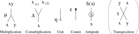
Figure 2: Operations in Hopf algebras

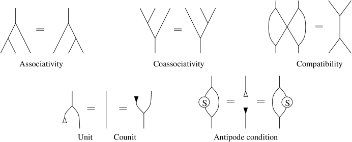
Figure 3: Axioms of Hopf algebras

Let $H$ be a Hopf algebra. Define $q:H\otimes H\rightarrow H$ by $q=\mu(1\otimes\mu)(S\otimes 1\otimes 1)(\tau\otimes 1)(1\otimes\Delta)$ where $\mu$, $\Delta,$ and $S$ denote the multiplication, comultiplication, and antipode, respectively. If we adopt the common notation $\Delta(x)=x_{(1)}\otimes x_{(2)}$ and $\mu(x\otimes y)=xy$, then $q$ is written as $q(x\otimes y)=S(y_{(1)})xy_{(2)}$. This appears as an adjoint map in [26, 20], and its diagram is depicted in Fig. 4. Notice the analogy with the group conjugation as a quandle: in a group ring, $\Delta(y)=y\otimes y$ and $S(y)=y^{-1}$, so that $q(x\otimes y)=y^{-1}xy$, and therefore, is of a great interest from point of view of quandles.

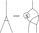
Figure 4: Self-distributive map in Hopf algebras

Figure 5: Proof of self-distributivity in Hopf algebras

Proposition 3.6

The above defined linear map $q:H\otimes H\rightarrow H$ satisfies the self-distributive law in Definition 2.1.

Proof. In Fig. 5, it is indicated that this follows from two properties of the adjoint map: $q(q\otimes 1)=q(1\otimes\mu)$ (which is used in the first and the third equalities in the figure), and $\mu=\mu(1\otimes q)(\tau\otimes 1)(1\otimes\Delta)$ (which is used in the second equality).

It is known that these properties are satisfied, and proofs are found in [26, 15]. Here we include diagrammatic proofs for reader’s convenience in Fig. 6 and Fig. 7, respectively. $\Box$

Remark 3.7

The definition of $q$ above contains an antipode, which is a coalgebra anti-homomorphism and not necessarily a coalgebra morphism. Thus, $(H,q)$ is not a shelf in ${\rm Coalg}$ in general.

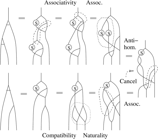
Figure 6: $q(q\otimes 1)=q(1\otimes\mu)$

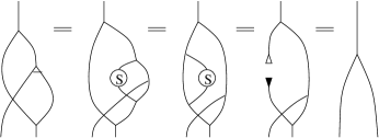
Figure 7: $\mu=\mu(1\otimes q)(\tau\otimes 1)(1\otimes\Delta)$

3.4 Other Examples

In this section we observe that there are plenty of examples of self-distributive linear maps for $2$-dimensional cocommutative coalgebras and shelves in ${\rm CoComCoalg}$.

Let $V$ be the two dimensional vector space over $k$ with basis $\{x,y\}$. Define a coalgebra structure on $V$ using the diagonal map $\Delta(z)=z\otimes z$ for $z\in\{x,y\}$ and extending it linearly.

Lemma 3.8

A linear map $q:V\otimes V\rightarrow V$ is self-distributive and compatible with comultiplication if and only if $q$ is a map defined on basis elements in the following list:

$$\begin{array}[]{ll|l|l|l|l|l|l|l|l|l|l|l|l|l|l|l|l|l|l|l|l}q(x\otimes x)=&0&0&0&0&0&0&x&x&x&x&x&x&x&x&x&y&y&y&y&y&0\\ q(x\otimes y)=&0&0&0&0&x&y&0&0&0&x&x&x&x&y&y&0&x&y&y&y&0\\ q(y\otimes x)=&0&0&x&x&0&0&0&0&y&x&x&y&y&x&y&0&y&0&x&y&0\\ q(y\otimes y)=&x&y&0&x&y&0&0&y&0&x&y&x&y&y&y&0&y&0&x&y&0\end{array}$$

Among these, $(V,q)$ is a shelf in ${\rm CoComCoalg}$ if and only if $q(a,b)\neq 0$ for any $a,b\in\{x,y\}.$

Proof. Let $q(x\otimes x)=\gamma_{1}x+\gamma_{2}y$ for some constants $\gamma_{1}$, $\gamma_{2}\in k$. The compatibility condition

$$\Delta q(x\otimes x)=(q\otimes q)(1\otimes\tau\otimes 1)(\Delta\otimes\Delta)(x\otimes x)$$

implies that $\gamma_{1}\gamma_{2}=0$ and $\gamma_{1}^{2}=\gamma_{1}$, $\gamma_{2}^{2}=\gamma_{2}$, i.e., $q(x\otimes x)=0$, $x$, or $y$. The same holds for $x\otimes y$, $y\otimes x$ and $y\otimes y$, so that the value of $q$ for a pair of basis elements is either a basis element ($x$ or $y$), or $0$.

A case by case analysis (facilitated by Mathematica and/or Maple) provides self-distributivity. When $\epsilon{(x)}=\epsilon{(y)}=1$, the only cases for which $\epsilon q=\epsilon\otimes\epsilon$ are those for which $q(a,b)\neq 0$ for all four choices of $a,b$. $\Box$

Another famous example of a cocommutative coalgebra is the trigonometric coalgebra, $T$, generated by $a$ and $b$ with comultiplication given by:

$$\Delta(a) = a\otimes a-b\otimes b$$

$$\Delta(b) = a\otimes b+b\otimes a$$

with counit $\epsilon(a)=1$, $\epsilon(b)=0$, in analogy with formulas for $\cos(x+y)$ and $\sin(x+y)$ and $\cos(0)=1$, $\sin(0)=0$.

Lemma 3.9

Let $T$ denote the trigonometric coalgebra over $\mathbb{C}$. Let $q:T\otimes T\rightarrow T$ be a linear map defined by:

$$q(a\otimes a)\ =\ \alpha_{1}a+\beta_{1}b, q(a\otimes b)\ =\ \alpha_{2}a+\beta_{2}b,$$

$$q(b\otimes a)\ =\ \alpha_{3}a+\beta_{3}b, q(b\otimes b)\ =\ \alpha_{4}a+\beta_{4}b.$$

Then such a linear map $q$ is self-distributive and compatible with comultiplication if and only if the coefficients are found in Table 1, where $i=\sqrt{-1}$.

Among these, $(V,q)$ is a shelf in ${\rm CoComCoalg}$ if and only if $(\alpha_{1},\alpha_{2},\alpha_{3},\alpha_{4})=(1,0,0,0)$.

Proof. This result is a matter of verifying the conditions for self-distributivity and compatibility over all possible choices of inputs. We generated solutions by both Maple and Mathematica. For the compatibility condition we established a system of $12$ quadratic equations in eight unknowns. Originally there were $16$ such equations, but $4$ of these are duplicates. In the Mathematica program we used the command “Solve” to generate a set of necessary conditions. The self-distributive condition gave a system of cubic equations in the unknowns. We checked these subject to the necessary conditions, and found the $21$ solutions above.

Expressing $\epsilon$ as a $(1\times 2)$ matrix and $q$ as the $2\times 4$ matrix $\left(\begin{array}[]{cccc}\alpha_{1}&\alpha_{2}&\alpha_{3}&\alpha_{4}\\ \beta_{1}&\beta_{2}&\beta_{3}&\beta_{4}\end{array}\right).$ We compute $\epsilon q=(\alpha_{1},\alpha_{2},\alpha_{3},\alpha_{4})$ and $\epsilon\otimes\epsilon=(1,0,0,0)$. The result follows. $\Box$

$$\begin{array}[]{||cccc||cccc||}\hline\cr\hline\cr\alpha_{1}&\alpha_{2}&\alpha_{3}&\alpha_{4}&\beta_{1}&\beta_{2}&\beta_{3}&\beta_{4}\\ \hline\cr\hline\cr 1&0&0&0&0&0&-1&0\\ \hline\cr 0&0&0&0&0&0&0&0\\ \hline\cr\frac{1}{2}&-\frac{i}{2}&0&0&0&0&\frac{1}{2}&-\frac{i}{2}\\ \hline\cr\frac{1}{2}&\frac{i}{2}&0&0&0&0&\frac{1}{2}&\frac{i}{2}\\ \hline\cr 1&0&0&0&0&0&1&0\\ \hline\cr\frac{1}{2}&0&0&-\frac{1}{2}&0&\frac{1}{2}&\frac{1}{2}&0\\ \hline\cr 1&0&0&0&0&1&0&0\\ \hline\cr\frac{1}{4}&-\frac{i}{4}&-\frac{i}{4}&-\frac{1}{4}&-\frac{i}{4}&-\frac{1}{4}&-\frac{1}{4}&\frac{i}{4}\\ \hline\cr\frac{1}{4}&\frac{i}{4}&-\frac{i}{4}&\frac{1}{4}&-\frac{i}{4}&\frac{1}{4}&-\frac{1}{4}&-\frac{i}{4}\\ \hline\cr\frac{1}{4}&\frac{i}{4}&\frac{i}{4}&-\frac{1}{4}&-\frac{i}{4}&\frac{1}{4}&\frac{1}{4}&\frac{i}{4}\\ \hline\cr\frac{1}{4}&\frac{i}{4}&\frac{i}{4}&-\frac{1}{4}&\frac{i}{4}&-\frac{1}{4}&-\frac{1}{4}&-\frac{i}{4}\\ \hline\cr\frac{1}{4}&-\frac{i}{4}&\frac{i}{4}&\frac{1}{4}&\frac{i}{4}&\frac{1}{4}&-\frac{1}{4}&\frac{i}{4}\\ \hline\cr\frac{1}{4}&-\frac{i}{4}&-\frac{i}{4}&-\frac{1}{4}&\frac{i}{4}&\frac{1}{4}&\frac{1}{4}&-\frac{i}{4}\\ \hline\cr 1&0&0&0&-\frac{i}{2}&-\frac{1}{2}&\frac{1}{2}&\frac{i}{2}\\ \hline\cr\frac{1}{2}&0&-\frac{i}{2}&0&-\frac{i}{2}&0&-\frac{1}{2}&0\\ \hline\cr 1&0&0&0&-\frac{i}{2}&\frac{1}{2}&\frac{1}{2}&-\frac{i}{2}\\ \hline\cr 1&0&0&0&\frac{i}{2}&-\frac{1}{2}&\frac{1}{2}&-\frac{i}{2}\\ \hline\cr\frac{1}{2}&0&\frac{i}{2}&0&\frac{i}{2}&0&-\frac{1}{2}&0\\ \hline\cr 1&0&0&0&\frac{i}{2}&\frac{1}{2}&\frac{1}{2}&\frac{i}{2}\\ \hline\cr 1&0&0&0&-i&0&0&0\\ \hline\cr 1&0&0&0&i&0&0&0\\ \hline\cr\hline\cr\end{array}$$

Table 1: List of self-distributive maps in the trigonometric coalgebra

4 Yang–Baxter Equation and Self-Distributive Maps for Coalgebras

In this section, we discuss relationships between solutions to the Yang-Baxter equations and self-distributive maps.

4.1 A Brief Review of YBE

The Yang–Baxter equation makes sense in any monoidal category. Originally mathematical physicists concentrated on solutions in the category of vector spaces with the tensor product, obtaining solutions from quantum groups.

Let $V$ be a vector space and $R:V\otimes V\rightarrow V\otimes V$ an invertible linear map. We say $R$ is a Yang–Baxter operator if it satisfies the Yang–Baxter equation, (YBE), which says that: $(R\otimes 1)(1\otimes R)(R\otimes 1)=(1\otimes R)(R\otimes 1)(1\otimes R)$. In other words, the YBE says that the following diagram commutes:

A solution to the YBE is also called a braiding.

In general, a braiding operation provides a diagrammatic description of the process of switching the order of two things. This idea is formalized in the concept of a braided monoidal category, where the braiding is an isomorphism

$$R_{X,Y}:X\otimes Y\rightarrow Y\otimes X.$$

If we draw $R:V\otimes V\rightarrow V\otimes V$ by the diagram:

then the Yang–Baxter equation is represented by:

This diagram represents the third Reidemeister move in classical knot theory [7], and it gives the most important relations in Artin’s presentation of the braid group [4]. As a result, any invertible solution of the Yang–Baxter equation gives an invariant of braids.

4.2 Shelves in Coalg and Solutions of the YBE

We now demonstrate the relationship between self-distributive maps in ${\rm Coalg}$ and solutions to the Yang–Baxter equation.

Figure 8: Solutions to YBE and shelves in Coalg

Definition 4.1

Let $X$ be a coalgebra and $q:X\otimes X\rightarrow X$ a linear map. Then the linear map $R_{q}:X\otimes X\rightarrow X\otimes X$ defined by

$$R_{q}=(1_{X}\otimes q)(\tau\otimes 1_{X})(1_{X}\otimes\Delta)$$

is said to be induced from $q$.

Conversely, let $R:X\otimes X\rightarrow X\otimes X$ be a linear map. Then the linear map $q_{R}:X\otimes X\rightarrow X$ defined by $q_{R}=(\epsilon\otimes 1_{X})R$ is said to be induced from $R$.

Figure 9: Hypotheses of Theorem 4.2

Diagrammatically, constructions of one of these maps from the other are depicted in Fig. 8. Our goal is to relate solutions of the YBE and self-distributive maps in certain categories via these induced maps.

Figure 10: Proof of Theorem 4.2

Figure 11: Cocommutativity

Theorem 4.2

Let $R:X\otimes X\rightarrow X\otimes X$ be a solution to the YBE on a coalgebra $X$ with counit. Suppose $R$ satisfies $(\epsilon\otimes\epsilon)R=(\epsilon\otimes\epsilon)$ and $R_{q_{R}}=R$. Then $(X,q_{R})$ is a shelf in ${\rm Coalg}.$

Proof. The conditions in the assumption are presented in Fig. 9. A proof is presented in Fig. 10. $\Box$

Figure 12: Proof of Theorem 4.3

Theorem 4.3

Let $X$ be an object in ${\rm CoComCoalg}$. Suppose a self-distributive linear map $q:X\otimes X\rightarrow X$ is compatible with comultiplication. Then $R_{q}$ is a solution to the YBE.

Proof. The cocommutativity of $\Delta$ is depicted in Fig. 11. A proof, then, is depicted in Fig. 12. Note here the condition that $q$ is compatible with comultiplication is that: $\Delta(q(a\otimes b))=q(a_{(1)}\otimes b_{(1)})\otimes q(a_{(2)}\otimes b_{(2)})$ or, equivalently, $\Delta q=q(1\otimes\tau\otimes 1)(\Delta\otimes\Delta)$. This is applied in Fig. 12 on the bottom row with the equal sign indicated to follow from compatibility. $\Box$

Propositions 3.1 and  3.5 and Theorem 4.3 imply the following:

Corollary 4.4

Let $q$ be a map defined from a quandle/rack as in Proposition 3.1 or from a Lie algebra as in Proposition 3.5. Then the induced map $R_{q}$ is a solution to the YBE.

In the Lie algebra case, the map is given as follows:

$$R_{q}((a,x)\otimes(b,y))=(b,y)\otimes(a,x)+(1,0)\otimes(0,[x,y]).$$

This appears, for example, in [12, 19].

Remark 4.5

Next we focus on the case of the adjoint map in Hopf algebras. Remark  3.7 states that the self-distributive map $q(x\otimes y)=S(y_{(1)})xy_{(2)}$ is not compatible with comultiplication, and therefore, Theorem 4.3 cannot be applied. However, the induced map $R_{q}$ does, indeed, satisfy YBE. This is of course for different reasons, and proved in [26], which was interpreted in [15] as a restriction of a regular representation of the universal $R$-matrix of a quantum double. Since it is of a great interest why the same construction gives rise to solutions to YBE for different reasons, we include their proofs in diagrams for reader’s convenience, and we specify two conditions from [26] in our point of view, to construct $R_{q}$ from $q$, and make a restatement of his theorem as follows:

Figure 13: Conclusion of Prop. 4.6/ Hypothesis of Prop. 4.7

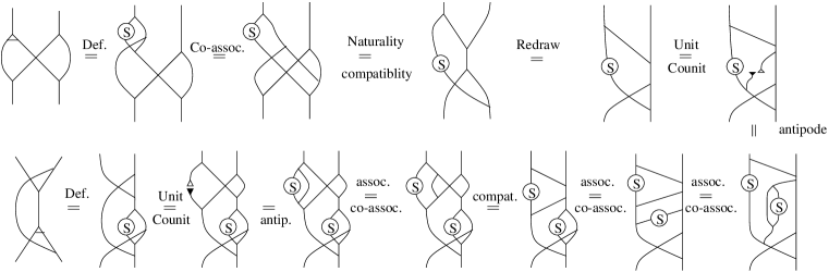
Figure 14: Proof of Proposition 4.6, second equation

Figure 15: Proof of Proposition 4.7

Proposition 4.6

In a Hopf algebra, let $q=\mu(1\otimes\mu)(S\otimes 1\otimes 1)(\tau\otimes 1)(1\otimes\Delta)$. Then $q(q\otimes 1)=q(1\otimes\mu)$ and $(q\otimes\mu)(1\otimes\tau\otimes 1)(\Delta\otimes\Delta)=(1\otimes\mu)(\tau\otimes 1)(1\otimes\Delta)(1\otimes q)(\tau\otimes 1)(1\otimes\Delta)$.

Proof. The proofs are indicated in Figs. 6 and  14, respectively. $\Box$

Recall from Section 3.3 that in a Hopf algebra, the map $q=\mu(1\otimes\mu)(S\otimes 1\otimes 1)(\tau\otimes 1)(1\otimes\Delta)$ satisfies self-distributivity.

Proposition 4.7

Suppose $X$ is a Hopf algebra and $q$ is any linear map that satisfies $q(q\otimes 1)=q(1\otimes\mu)$ and $(q\otimes\mu)(1\otimes\tau\otimes 1)(\Delta\otimes\Delta)=(1\otimes\mu)(\tau\otimes 1)(1\otimes\Delta)(1\otimes q)(\tau\otimes 1)(1\otimes\Delta)$. Then $R_{q}$ is a solution to the YBE.

Proof. The required conditions are depicted in Fig. 13. And the proof is given in Fig. 15. $\Box$

In particular, the above proposition applies when $q(x\otimes y)=S(y_{(1)})xy_{(2)}.$

5 Graph Diagrams for Bialgebra Hochschild Cohomology

The analogue of group cohomology for associative algebras is Hochschild cohomology. Then a natural question is, “What is an analogue of quandle cohomology for shelves in ${\rm Coalg}$?” Since we have developed diagrammatic methods to study self-distributivity in ${\rm Coalg},$ we apply these methods to seek such a cohomology theory, in combination with the interpretations of cocycles in bialgebra cohomology in terms of deformation theory of bialgebras. The first step toward this goal is to reestablish diagrammatic methods for Hochschild cohomology in terms of graph diagrams. Such approaches are found for homotopy Lie algebras and operads [21]. On the other hand, a diagrammatic method using polyhedra for bialgebra cohomology was given in [22]. In this section we follow the exposition in [22] of cocycles that appear in bialgebra deformation theory, and establish tree diagrams that can be used to prove cocycle conditions.

First we recall the Hochschild cohomology for bialgebras from [22]. Let $A=(V,\mu,\Delta)$ be a bialgebra over a field $k$, where $\mu$, $\Delta$ are multiplication and comultiplication, respectively, and $d_{H}:\mbox{Hom}(V^{\otimes p},V^{\otimes q})\rightarrow\mbox{Hom}(V^{\otimes(p+1)},V^{\otimes q})$ is the Hochschild differential

$$d_{H}(f)=\mu(1\otimes f)+\sum_{i=0}^{p-1}(-1)^{i+1}f(1^{i}\otimes\mu\otimes 1^{n-i-1})+(-1)^{p+1}\mu(f\otimes 1)$$

where the left and right module structures are given by multiplication. Dually $d_{C}:\mbox{Hom}(V^{\otimes p},V^{\otimes q})\rightarrow\mbox{Hom}(V^{\otimes p},V^{\otimes(q+1)})$ denotes the coHochschild differential. These define the total complex $(C^{*}_{b}(A;A),D)$, where $C^{n}_{b}(A;A)=\oplus_{i=1}^{n}\mbox{Hom}(V^{\otimes(n-i+1)},V^{\otimes i})$. For example, for a $1$-cochain $f\in\mbox{Hom}(V,V)$, $d_{H}(f)(x\otimes y)=xf(y)-f(xy)+f(x)y$ and $d_{C}(f)(x)=x_{(1)}\otimes f(x_{(2)})-f(x)_{(1)}\otimes f(x)_{(2)}+f(x_{(1)})\otimes x_{(2)}$.

For the rest of this section, we establish graph diagrams for Hochschild cohomology and review their aspects in deformation theory of bialgebras.

5.1 Graph Diagrams for Hochschild Differentials

A $1$-cochain $f\in\mbox{Hom}(V,V)$ is represented by a circle on a vertical segment as shown in Fig. 16, where the images of $f$ under the first differentials $d_{H}(f)$ and $d_{C}(f)$, as computed above, are also depicted. In general, a $(m+n-1)$-cochain in $\mbox{Hom}(V^{\otimes m},V^{\otimes n})$ is represented by a diagram in Fig. 17.

Figure 16: Hochschild $1$-differentials

Figure 17: Hochschild $(m+n)$-cochains

For $(\phi_{1},\phi_{2})$, where $\phi_{1}\in\mbox{Hom}(V^{\otimes 2},V)$ and $\phi_{2}\in\mbox{Hom}(V,V^{\otimes 2})$, the differentials are

$$d_{H}(\phi_{1}) = \mu(1\otimes\phi_{1})-\phi_{1}(\mu\otimes 1)+\phi_{1}(1\otimes\mu)-\mu(\phi_{1}\otimes 1),$$ (1)

$$d_{C}(\phi_{1}) = (\mu\otimes\phi_{1})\tau_{2}(\Delta\otimes\Delta)-\Delta(\phi_{1})+(\phi_{1}\otimes\mu)\tau_{2}(\Delta\otimes\Delta),$$ (2)

$$d_{H}(\phi_{2}) = (\mu\otimes\mu)\tau_{2}(\Delta\otimes\phi_{2})-\phi_{2}\mu+(\mu\otimes\mu)\tau_{2}(\phi_{2}\otimes\Delta),$$ (3)

$$d_{C}(\phi_{2}) = (1\otimes\phi_{2})\Delta-(\Delta\otimes 1)(\phi_{2})+(1\otimes\Delta)(\phi_{2})-(\phi_{2}\otimes 1)\Delta,$$ (4)

where $\tau_{2}$ is the homomorphism induced from the transposition of the second and the third factors. The $2$-cocycle conditions are $d_{H}(\phi_{1})=0$, $d_{C}(\phi_{1})=d_{H}(\phi_{2})$, and $d_{C}(\phi_{2})=0$. The differential $D$ of the total complex is $D=d_{H}-d_{C}$, $D(\phi_{1},\phi_{2})=d_{H}(\phi_{1})+[d_{H}(\phi_{2})-d_{C}(\phi_{1})]-d_{C}(\phi_{2})$.

Figure 18: Hochschild $2$-differentials

We demonstrate a proof that $(\phi_{1},\phi_{2})=(d_{H}(f),d_{C}(f))$ satisfies $d_{C}(\phi_{1})=d_{H}(\phi_{2})$ using graph diagrams. First, we use encircled vertices as depicted in Fig. 17 to represent an element of $\mbox{Hom}(V^{\otimes m},V^{\otimes n})$. Then $d_{C}(\phi_{1})$ and $d_{H}(\phi_{2})$ are represented on the top line of Fig. 18. Substituting $(\phi_{1},\phi_{2})=(d_{H}(f),d_{C}(f))$, that are represented diagrammatically as in Fig. 16, we perform diagrammatic computations as in the rest of Fig. 18, and the equality follows because multiplication and comultiplication are compatible. In particular each diagram in the left of the figure for which the vertex is external to the operations corresponds to a similar diagram on the right, but the correspondence is given after considering the compatible structures.

Figure 19: Hochschild $3$-cocycle conditions

For $3$-cochains $\psi_{i}\in\mbox{Hom}(V^{\otimes 3},V)$, $\psi_{2}\in\mbox{Hom}(V^{\otimes 2},V^{\otimes 2})$ and $\psi_{3}\in\mbox{Hom}(V,V^{\otimes 3})$, the $3$-cocycle condition is explicitly written as $d_{H}(\psi_{1})=0$, $d_{C}(\psi_{1})=d_{H}(\psi_{2})$, $d_{C}(\psi_{2})=d_{H}(\psi_{3})$, and $d_{C}(\psi_{3})=0$, see [22]

$$d_{H}(\psi_{1}) = \mu(1\otimes\psi_{1})-\psi_{1}(\mu\otimes 1^{2})+\psi_{1}(1\otimes\mu\otimes 1)-\psi_{1}(1^{2}\otimes\mu)+\mu(\psi_{1}\otimes 1),$$

$$d_{C}(\psi_{1}) = (\mu(1\otimes\mu)\otimes\psi_{1})\tau(\Delta\otimes\Delta\otimes\Delta)-\Delta(\psi_{1})+(\psi_{1}\otimes\mu(\mu\otimes 1))\tau(\Delta\otimes\Delta\otimes\Delta),$$

$$d_{H}(\psi_{2}) = (\mu\otimes\mu)\tau_{2}(\Delta\otimes\psi_{2})-\psi_{2}(\mu\otimes 1)+\psi_{2}(1\otimes\mu)-(\mu\otimes\mu)\tau_{2}(\psi_{2}\otimes\Delta),$$

$$d_{C}(\psi_{2}) = (\mu\otimes\psi_{2})\tau_{2}(\Delta\otimes\Delta)-(\Delta\otimes 1)(\psi_{2})+(1\otimes\Delta)(\psi_{2})-(\psi_{2}\otimes\mu)\tau_{2}(\Delta\otimes\Delta),$$

$$d_{H}(\psi_{3}) = (\mu\otimes\mu\otimes\mu)\tau^{\prime}((1\otimes\Delta)\Delta\otimes\psi_{3})-\psi_{3}(\mu)+(\mu\otimes\mu\otimes\mu)\tau^{\prime}(\psi_{3}\otimes(\Delta\otimes 1)\Delta),$$

$$d_{C}(\psi_{3}) = (1\otimes\psi_{3})\Delta-(\Delta\otimes 1^{2})(\psi_{3})+(1\otimes\Delta\otimes 1)(\psi_{3})-(1^{2}\otimes\Delta)(\psi_{3})+(\psi_{3}\otimes 1)\Delta,$$

where $\tau=\tau_{4}\tau_{3}\tau_{2}$ and $\tau^{\prime}=\tau_{5}\tau_{2}\tau_{3}$. In general, $\tau_{i}$ indicates the transposition of the $i\/$th and $(i+1)\/$st factors; the notation is used when type-setting gets complicated.

The first two $3$-cocycle conditions, $d_{H}(\psi_{1})=0$ and $d_{C}(\psi_{1})=d_{H}(\psi_{2})$, are depicted in Fig. 19. Note that the first is the pentagon identity for associativity. In particular, $\psi_{1}$ can be regarded as an obstruction to associativity. The morphism $\psi_{1}$ is assigned the difference between the two diagrams that represent the two expressions $(ab)c$ and $a(bc)$. Thus $\psi_{1}$ and its diagram are assigned to the change of diagrams corresponding to associativity, and can be seen to form an actual pentagon, as depicted in Fig. 20.

Figure 20: Hochschild $3$-cocycles as movies, part I

Similarly, the second condition $d_{C}(\psi_{1})=d_{H}(\psi_{2})$ can be represented as sequence of applications of the associativity and compatibility conditions as depicted in Fig. 21. Furthermore, the relations $d_{C}(\psi_{2})=d_{H}(\psi_{3})$ and $d_{C}(\psi_{3})=0$ can be obtained by turning the equations in Fig. 19 upside-down. Similarly, the “movie-moves” in Figs. 20 and 21 can be turned upside-down. Thus, $d_{C}(\psi_{3})=0$ when the pentagon identity for coassociativity holds, and $d_{C}(\psi_{2})=d_{H}(\psi_{3})$ when compatibility and coassociativity are compared.

Figure 21: Hochschild $3$-cocycles as movies, part Il

5.2 Review of Cocycles in Deformation Theory

Next we follow [22] for deformation of bialgebras. A deformation of $A=(V,\mu,\Delta)$ is a $k[[t]]$-bialgebra $A_{t}=(V_{t},\mu_{t},\Delta_{t})$, where $V_{t}=V\otimes k[[t]]$ and $A_{t}/(tA_{t})\cong A$. Deformations of $\mu$ and $\Delta$ are given by $\mu_{t}=\mu+t\mu_{1}+\cdots+t^{n}\mu_{n}+\cdots:V_{t}\otimes V_{t}\rightarrow V_{t}$ and $\Delta_{t}=\Delta+t\Delta_{1}+\cdots+t^{n}\Delta_{n}+\cdots:V_{t}\rightarrow V_{t}\otimes V_{t}$ where $\mu_{i}:V\otimes V\rightarrow V$, $\Delta_{i}:V\rightarrow V\otimes V$, $i=1,2,\cdots$, are sequences of maps. Suppose $\bar{\mu}=\mu+\cdots+t^{n}\mu_{n}$ and $\bar{\Delta}=\Delta+\cdots+t^{n}\Delta_{n}$ satisfy the bialgebra conditions (associativity, compatibility, and coassociativity) mod $t^{n+1}$, and suppose that there exist $\mu_{n+1}:V\otimes V\rightarrow V$ and $\Delta_{n+1}:V\rightarrow V\otimes V$ such that $\bar{\mu}+t^{n+1}\mu_{n+1}$ and $\bar{\Delta}+t^{n+1}\Delta_{n+1}$ satisfy the bialgebra conditions mod $t^{n+2}$. Define $\psi_{1}\in\mbox{Hom}(V^{\otimes 3},V)$, $\psi_{2}\in\mbox{Hom}(V^{\otimes 2},V^{\otimes 2})$, and $\psi_{3}\in\mbox{Hom}(V,V^{\otimes 3})$ by

$$\bar{\mu}(\bar{\mu}\otimes 1)-\bar{\mu}(1\otimes\bar{\mu}) = t^{n+1}\psi_{1}\quad{\rm mod}\ t^{n+2},$$ (5)

$$\bar{\Delta}\bar{\mu}-(\bar{\mu}\otimes\bar{\mu})\tau_{2}(\bar{\Delta}\otimes\bar{\Delta}) = t^{n+1}\psi_{2}\quad{\rm mod}\ t^{n+2},$$ (6)

$$(\bar{\Delta}\otimes 1)\bar{\Delta}-(1\otimes\bar{\Delta})\bar{\Delta} = t^{n+1}\psi_{3}\quad{\rm mod}\ t^{n+2}.$$ (7)

For the associativity of $\bar{\mu}+t^{n+1}\mu_{n+1}$ mod $t^{n+2}$ we obtain:

$$(\bar{\mu}+t^{n+1}\mu_{n+1})((\bar{\mu}+t^{n+1}\mu_{n+1})\otimes 1)-(\bar{\mu}+t^{n+1}\mu_{n+1})(1\otimes(\bar{\mu}+t^{n+1}\mu_{n+1}))=0\ {\rm mod}\ t^{n+2}$$

which is equivalent by degree calculations to:

$$d_{H}(\mu_{n+1})=\mu(1\otimes\mu_{n+1})-\mu_{n+1}(\mu\otimes 1)+\mu_{n+1}(1\otimes\mu_{n+1})-\mu(\mu_{n+1}\otimes 1)=\psi_{1}.$$

Similarly, we obtain: $(\psi_{1},\psi_{2},\psi_{3})=D(\mu_{n+1},\Delta_{n+1})$. The cochains $(\psi_{1},\psi_{2},\psi_{3})$, defined by deformations (5,6,7) then, satisfy the $3$-cocycle condition $D(\psi_{1},\psi_{2},\psi_{3})=0$. This concludes the review of deformation for the $2$-cocycle conditions cited from [22].

6 Towards a Cohomology Theory for Shelves in Coalg

Let $(X,q)$ be a coalgebra with a self-distributive linear map. In this section we present low-dimensional cocycle conditions for $q$. We justify our cocycle conditions through the use of analogy with Hochschild bialgebra cohomology using diagrammatics and the deformation theories reviewed in the preceding section. Both analogies are used interchangeably throughout this section, both in definitions and computations.

6.1 Chain Groups

Following the diagrammatics of the preceding section, we define chain groups, for positive integers $n$ and $i=1,\ldots,n$ by:

$$C^{n,i}_{\rm sh}(X;X) = \mbox{Hom}(X^{\otimes(n+1-i)},X^{\otimes i}),$$

$$C^{n}_{\rm sh}(X;X) = \oplus_{i=1}^{n}C^{n,i}_{sh}(X;X).$$

Specifically, the chain groups in low dimensions of our concern are:

$$C^{1}_{\rm sh}(X;X) = \mbox{Hom}(X,X),$$

$$C^{2}_{\rm sh}(X;X) = \mbox{Hom}(X^{\otimes 2},X)\oplus\mbox{Hom}(X,X^{\otimes 2}),$$

$$C^{3}_{\rm sh}(X;X) = \mbox{Hom}(X^{\otimes 3},X)\oplus\mbox{Hom}(X^{\otimes 2},X^{\otimes 2})\oplus\mbox{Hom}(X,X^{\otimes 3}).$$

To help keep track of the chain groups and their indices, we include the diagram in Fig. 22. The chain groups $C^{n,i}$ are located at position $(n+2-i,i)$ in the positive quadrant of the integer lattice. The chain groups $C^{j}$ are the direct sum of the groups along lines of slope $(-1)$. Differentials in the figure are indicated by arrows that point to the target groups. The differential $d^{2,3}$ has as its source the summand $C^{2,2}\subset C^{2}$ as indicated.

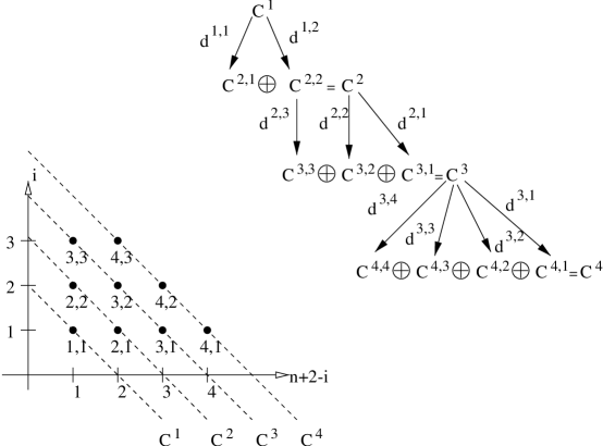
Figure 22: The lattice of chain groups and differentials

In the remaining sections we will define differentials that are homomorphisms between the chain groups:

$$d^{n,i}:C^{n}_{\rm sh}(X;X)\rightarrow C^{n+1,i}_{\rm sh}(X;X)(=\mbox{Hom}(X^{\otimes(n+2-i)},X^{\otimes i}))$$

and will be defined individually for $n=1,2,3$ and $i=1,\ldots,n+1$, and

$$D_{1} = d^{1,1}-d^{1,2}:C^{1}_{\rm sh}(X;X)\rightarrow C^{2}_{\rm sh}(X;X),$$

$$D_{2} = d^{2,1}+d^{2,2}+d^{2,3}:C^{2}_{\rm sh}(X;X)\rightarrow C^{3}_{\rm sh}(X;X),$$

$$D_{3} = d^{3,1}+d^{3,2}+d^{3,3}+d^{3,4}:C^{3}_{\rm sh}(X;X)\rightarrow C^{3}_{\rm sh}(X;X).$$

6.2 First Differentials

We take

$$d^{1,2}:\mbox{Hom}(X;X)(=C^{1,1}_{\rm sh}(X;X))\rightarrow\mbox{Hom}(X,X^{\otimes 2})(=C^{2,2}_{\rm sh}(X;X))$$

to be the coHochschild differential for the comultiplication $d^{1,2}(f)=(1\otimes f)\Delta-\Delta f+(f\otimes 1)\Delta$. Again by analogy with the differential for multiplication, we take:

$$d^{1,1}:\mbox{Hom}(X,X)(=C^{1,1}_{\rm sh}(X;X))\rightarrow\mbox{Hom}(X^{\otimes 2},X)(=C^{2,1}_{\rm sh}(X;X))$$

to be $d^{1,1}(f)=q(1\otimes f)-fq+q(f\otimes 1)$. Then define $D_{2}:C^{1}_{\rm sh}(X;X)\rightarrow C^{2}_{\rm sh}(X;X)$ by $D_{1}=d^{1,1}-d^{1,2}$.

6.3 Second Differentials

We derive second differentials by analogy with deformation theory, and then show that our definitions carry through in diagrammatics.

Recall that the self-distributivity, compatibility, and coassociativity are written as:

$$q(q\otimes 1) = q(q\otimes q)\tau_{2}(1\otimes 1\otimes\Delta),$$

$$\Delta q = (q\otimes q)\tau_{2}(\Delta\otimes\Delta),$$

$$(\Delta\otimes 1)\Delta = (1\otimes\Delta)\Delta.$$

where $\tau_{2}$ is the transposition acting on the second and third tensor factors. As before let $X_{t}=X\otimes k[[t]]$ and suppose we have partial deformations $\bar{q}=q+\cdots+t^{n}q_{n}$ and $\bar{\Delta}=\Delta+\cdots+t^{n}\Delta_{n}$ satisfying the above three conditions mod $t^{n+1}$, and suppose there are $q_{n+1}$ and $\Delta_{n+1}$ such that $\bar{q}+q_{n+1}$ and $\bar{\Delta}+\Delta_{n+1}$ satisfy the three conditions mod $t^{n+2}$.

Setting

$$\bar{q}(\bar{q}\otimes 1)-\bar{q}(\bar{q}\otimes\bar{q})\tau_{2}(1\otimes 1\otimes\bar{\Delta}) = t^{n+1}\xi_{1}\quad{\rm mod}\ t^{n+2},$$

$$\bar{\Delta}\bar{q}-(\bar{q}\otimes\bar{q})\tau_{2}(\bar{\Delta}\otimes\bar{\Delta}) = t^{n+1}\xi_{2}\quad{\rm mod}\ t^{n+2},$$

$$(\bar{\Delta}\otimes 1)\bar{\Delta}-(1\otimes\bar{\Delta})\bar{\Delta} = t^{n+1}\xi_{3}\quad{\rm mod}\ t^{n+2},$$

we obtain:

$$\left[q(q_{n+1}\otimes 1)+q_{n+1}(q\otimes 1)\right]-\left[q_{n+1}(q\otimes q)\tau_{2}(1\otimes 1\otimes\Delta)+q(q_{n+1}\otimes q)\tau_{2}(1\otimes 1\otimes\Delta)+\right.$$

$$\left.q(q\otimes q_{n+1})\tau_{2}(1\otimes 1\otimes\Delta)+q(q\otimes q)\tau_{2}(1\otimes 1\otimes\Delta_{n+1})\right] = \xi_{1},$$

$$\left[\Delta q_{n+1}+\Delta_{n+1}q\right]-\left[(q_{n+1}\otimes q)\tau_{2}(\Delta\otimes\Delta)+(q\otimes q_{n+1})\tau_{2}(\Delta\otimes\Delta)+\right.$$

$$\left.(q\otimes q)\tau_{2}(\Delta_{n+1}\otimes\Delta)+(q\otimes q)\tau_{2}(\Delta\otimes\Delta_{n+1})\right] = \xi_{2},$$

$$\left[(\Delta_{n+1}\otimes 1)\Delta+(\Delta\otimes 1)\Delta_{n+1}\right]-\left[(1\otimes\Delta_{n+1})\Delta+(1\otimes\Delta)\Delta_{n+1}\right] = \xi_{3}.$$

A natural requirement is $D_{2}(q_{n+1},\Delta_{n+1})=(\xi_{1},\xi_{2},\xi_{3})$, so we define $D_{2}:C^{2}_{\rm sh}(X;X)\rightarrow C^{3}_{\rm sh}(X;X)$ by $D_{2}=d^{2,1}+d^{2,2}+d^{2,3}$, where

$$d^{2,1}(\eta_{1},\eta_{2}) = \left[q(\eta_{1}\otimes 1)+\eta_{1}(q\otimes 1)\right]-\left[\eta_{1}(q\otimes q)\tau_{2}(1\otimes 1\otimes\Delta)+q(\eta_{1}\otimes q)\tau_{2}(1\otimes 1\otimes\Delta)\right.$$

$$\left.\quad+q(q\otimes\eta_{1})\tau_{2}(1\otimes 1\otimes\Delta)+q(q\otimes q)\tau_{2}(1\otimes 1\otimes\eta_{2})\right]$$

$$d^{2,2}(\eta_{1},\eta_{2}) = \left[\Delta\eta_{1}+\eta_{2}q\right]-\left[(\eta_{1}\otimes q)\tau_{2}(\Delta\otimes\Delta)+(q\otimes\eta_{1})\tau_{2}(\Delta\otimes\Delta)\right.$$

$$\left.\quad+(q\otimes q)\tau_{2}(\eta_{2}\otimes\Delta)+(q\otimes q)\tau_{2}(\Delta\otimes\eta_{2})\right]$$

$$d^{2,3}(\eta_{1},\eta_{2}) = \left[(\eta_{2}\otimes 1)\Delta+(\Delta\otimes 1)\eta_{2}\right]-\left[(1\otimes\eta_{2})\Delta+(1\otimes\Delta)\eta_{2}\right].$$

In fact, $d^{2,3}=d_{C}$, the same as the coHochschild $2$-differential for the comultiplication.

Figure 23: Diagrams for $2$-cochains

The diagrammatic conventions for $q$, a $2$-cochain $\eta_{1}\in\mbox{Hom}(X^{\otimes 2},X)$, and $\Delta$, a $2$-cochain $\eta_{2}\in\mbox{Hom}(X,X^{\otimes 2})$ are depicted from left to right, respectively, in Fig. 23.

Figure 24: The first $2$-differential $d^{2,1}$

Figure 25: The second $2$-differential $d^{2,2}$

The first and second differentials $d^{2,1}(\eta_{1},\eta_{2})$, $d^{2,2}(\eta_{1},\eta_{2})$ are depicted in Fig. 24 and Fig. 25, respectively. Here we note that these diagrams agree with those for Hochschild bialgebra cohomology in the sense that they are obtained by the following process: (1) Consider the diagrams of the equality in question (in this case the self-distributivity condition and the compatibility), (2) Mark exactly one vertex of such a diagram, (3) Take a formal sum of such diagrams over all possible markings. In Fig. 24, the first two terms correspond to the LHS of $q(q\otimes 1)=q(q\otimes q)\tau_{2}(1^{2}\otimes\Delta)$, and one of the two white triangular vertices is marked by a black vertex, representing the $2$-cochain $\eta_{1}$, while the remaining white vertex represents $q$. The negative four terms correspond to the RHS, and the last term has a circle, representing $\eta_{2}$ while unmarked ones in the rest represent $\Delta$. The same procedure for the compatibility gives rise to Fig. 25.

Figure 26: $d^{2,1}(D_{1}(f))=0$

Figure 27: $d^{2,2}(D_{1}(f))=0$

Lemma 6.1

For any $f\in C^{1}_{\rm sh}(X;X)$, we have $D_{2}D_{1}(f)=0$.

Proof. A proof is depicted in Fig. 26 and Fig. 27. By assumption, $\eta_{1}=d^{1,1}(f)$ and $\eta_{2}=d^{1,2}(f)$. Therefore, as in the case of Hochschild homology, marked vertices representing $\eta_{1}$ and $\eta_{2}$ are replaced by formal sum of three diagrams representing $d^{1,1}(f)$ and $d^{1,2}(f)$, see Fig. 16. The situation in which the first two terms are replaced by three terms each is depicted in the top two lines of Fig. 26.

A white circle on an edge represents $f$. The bottom three lines show replacements for the remaining four negative terms. Then the terms represented by identical graphs cancel directly. If a white circle representing $f$ appears near the boundary, then we use the self-distributive axiom to relate this to another term. For example, the first term on the top left cancels with the third term on the bottom row since $f$ is on the second tensor factor at the bottom of each.

To facilitate the reader’s understanding of the computation we present the following sequences: $1,-2,3,4,-5,2$ and $-6,5,-7,-8,7,-3,-9,6,-1,9,-4,8.$ Label the diagrams below the arrows in Fig. 26 in order with these numbers. The minus sign indicates the sign of the given term on the given side of the equation, and the number indicates which diagrams cancel which. A similar labelling can be accomplished in Fig. 27. $\Box$

Figure 28: First $3$-differential, $d^{3,1}$

We also note the following restricted version:

Lemma 6.2

Let $f\in C^{1}_{\rm sh}(X;X)=\mbox{Hom}(X;X)$. If $d^{1,2}(f)=0\in C^{2,2}_{\rm sh}(X;X)=\mbox{Hom}(X;X^{\otimes 2})$, then $D_{2}(d^{1,1}(f),0)=0$.

Proof. The conclusion is restated by the following condition: $d^{2,i}(d^{1,1}(f),0)=0$ for $i=1,2$, since $d^{1,1}(f)$ is not in the domain of the differential $d^{2,3}$. Then one computes $d^{2,i}(\eta_{1},0)$ for $\eta_{1}=d^{1,1}(f)$ either directly, or diagrammatically using Figs. 26, and 27, without trivalent vertices that are encircled. $\Box$

Figure 29: Second $3$-differential, $d^{3,2}$

6.4 Third Differentials

Throughout this section, we consider only self-distributive linear maps for cocommutative coalgebras with counits. The maps $q$ need not be compatible with the counit, but there must be such a counit present. In this case, $3$-differentials

$$d^{3,i}:C^{3}_{\rm sh}(X;X)(=\oplus_{j=1}^{3}\mbox{Hom}(X^{\otimes(4-j)},X^{\otimes j}))\rightarrow C^{4,i}_{\rm sh}(X;X)(=\mbox{Hom}(X^{\otimes(n+2-i)},X^{\otimes i}))$$

are defined below for $i=1,2,3$, and for $i=4$ it is defined by the same map as the differential for $\Delta$ for co-Hochschild cohomology (the pentagon identity for the comultiplication). Let $\xi_{j}\in\mbox{Hom}(X^{\otimes(4-j)},X^{\otimes j})\subset C^{3}_{\rm sh}(X;X)$, $j=1,2,3$.

Figure 30: Third $3$-differential, $d^{3,3}$

These differentials are defined by direct analogues with Hochschild differentials in diagrammatics, and we will justify our definition in two more ways: (1) $2$-cochains vanish under these maps, (2) $3$-cocycles of quandle and Lie algebra cohomology are realized in these formulas as discussed in the next section.

First we explain the diagrammatics. Recall that $3$-cocycle conditions in Hochschild cohomology correspond to two different sequences of relations applied to graphs that change one graph to another. At the top of Fig. 28, a graph representing $q(q\otimes 1)(q\otimes 1^{2})$ is depicted. There are two ways to apply sequences of self-distributivity to this map to get the map represented by the bottom graphs. A $3$-cochain $\xi_{1}$ represented by a black triangular vertex with three bottom edges and a single top edge corresponds to applying the self-distributivity relation to change a graph to another, and corresponds to where the self-distributivity relation was applied. The two different sequences are shown at the left and right of the figure. These sequences give rise to the LHS and RHS of $d^{3,1}(\xi_{1},\xi_{2},\xi_{3})$. Similar graphs are obtained as shown in Figs. 29 and 30.

The differentials thus obtained are:

$$d^{3,1}(\xi_{1},\xi_{2},\xi_{3}) = [q(\xi_{1}\otimes 1)+\xi_{1}(q\otimes q\otimes 1)(1\otimes\tau\otimes 1^{2})(1^{2}\otimes\Delta\otimes 1)$$

$$+\ \ q(\xi_{1}\otimes q)(1^{2}\otimes\tau\otimes 1)(1^{3}\otimes\Delta)(1^{2}\otimes q\otimes 1)$$

$$(1\otimes\tau\otimes 1^{2})(1^{2}\otimes\Delta\otimes 1)$$

$$+\ \ q(q\otimes\xi_{1})(q\otimes q\otimes 1^{3})(1\otimes\tau\otimes 1^{4})$$

$$(1^{2}\otimes\Delta\otimes 1^{3})(1^{2}\otimes\tau\otimes 1^{2})(1\otimes\tau\otimes\tau\otimes 1)(1^{2}\otimes\Delta\otimes\Delta)$$

$$+\ q(q\otimes q)(q\otimes q\otimes q\otimes q)(1\otimes\tau\otimes 1^{2}\otimes\tau\otimes 1)(1^{2}\otimes\Delta\otimes 1^{3})$$

$$(1^{2}\otimes\tau\otimes 1^{2})(1\otimes\tau\otimes\tau\otimes 1^{2})(1^{2}\otimes\Delta\otimes\xi_{3})]$$

$$-\ [\xi_{1}(q\otimes 1^{2})+q(\xi_{1}\otimes q)(1^{2}\otimes\tau\otimes 1)(1^{3}\otimes\Delta)$$

$$+\ \ \xi_{1}(q\otimes q\otimes q)(1\otimes\tau\otimes 1^{3})(1^{2}\otimes\Delta\otimes 1^{2})(1^{2}\otimes\tau\otimes 1)(1^{3}\otimes\Delta)$$

$$+\ \ q(q\otimes q)(1\otimes\tau\otimes 1)(q\otimes q\otimes 1^{2})(1^{2}\otimes\Delta\otimes 1^{2})(1^{3}\otimes\xi_{2})(1^{2}\otimes\tau\otimes 1)(1^{3}\otimes\Delta)$$

$$+\ q(q\otimes q)(q\otimes q\otimes q\otimes q)(1\otimes\tau\otimes\tau\otimes 1^{3})(1^{4}\otimes\tau\otimes\tau\otimes 1^{2})$$

$$(1\otimes\tau\otimes\Delta\otimes\tau\otimes 1)(1^{2}\otimes\Delta\otimes\xi_{3})]$$

$$d^{3,2}(\xi_{1},\xi_{2},\xi_{3}) = [\Delta\xi_{1}+\xi_{2}(q\otimes q)(1\otimes\tau\otimes 1)(1^{2}\otimes\Delta)$$

$$+\ \ (q\otimes q)(1\otimes\tau\otimes 1)(\xi_{2}\otimes\Delta)(1^{2}\otimes q)(1\otimes\tau\otimes 1)(1^{2}\otimes\Delta)$$

$$+\ (q\otimes q)(1\otimes\tau\otimes 1)(\Delta\otimes 1^{2}))(q\otimes\xi_{2})(1\otimes\tau\otimes 1)(1^{2}\otimes\Delta)$$

$$+\ (q\otimes q)(q\otimes\tau\otimes q)(1^{2}\otimes q\otimes q\otimes 1^{2})(1\otimes\tau\otimes\tau\otimes\tau\otimes 1)$$

$$(\Delta\otimes 1^{2}\otimes\tau\otimes\Delta)(1\otimes\tau\otimes 1^{3})(1\otimes\Delta\otimes\xi_{3})]$$

$$- [\xi_{2}(q\otimes 1)+(q\otimes q)(1\otimes\tau\otimes 1)(\xi_{2}\otimes\Delta)$$

$$+\ \ (\xi_{1}\otimes q)(1^{3}\otimes q\otimes 1)(1^{2}\otimes\tau\otimes 1^{2})(1\otimes\tau\otimes\tau\otimes 1)(\Delta\otimes\Delta\otimes\Delta)$$

$$+\ \ (q\otimes\xi_{1})(q\otimes 1^{4})(1^{2}\otimes\tau\otimes 1^{2})(1\otimes\tau\otimes\tau\otimes 1)(\Delta\otimes\Delta\otimes\Delta)$$

$$+\ \ (q\otimes q)(q\otimes q\otimes q\otimes q)(1\otimes\tau\otimes\tau\otimes\tau\otimes 1)(1^{2}\otimes\tau\otimes\tau\otimes\Delta)$$

$$(1\otimes\tau\otimes\tau\otimes 1^{2})(\Delta\otimes\Delta\otimes\xi_{3})]$$

$$d^{3,3}(\xi_{1},\xi_{2},\xi_{3}) = [(\Delta\otimes 1)\xi_{2}+(\xi_{2}\otimes q)(1\otimes\tau\otimes 1)(\Delta\otimes\Delta)$$

$$+\ \ (q\otimes q\otimes q)(1\otimes\tau\otimes 1^{3})(1^{2}\otimes\Delta\otimes 1^{2})(1^{2}\otimes\tau\otimes 1^{2})(\xi_{3}\otimes\Delta)]$$

$$- [\xi_{3}q+(1\otimes\Delta)\xi_{2}+(q\otimes\xi_{2})(1\otimes\tau\otimes 1)(\Delta\otimes\Delta)$$

$$+\ \ (q\otimes q\otimes q)(1\otimes\tau\otimes\tau\otimes 1)(1^{2}\otimes\tau\otimes 1^{2})(1\otimes\Delta\otimes 1^{3})(\Delta\otimes\xi_{3})]$$

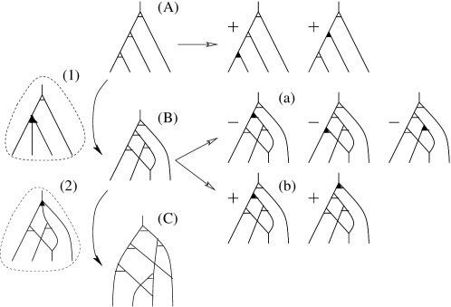
Figure 31: A strategy for a proof

The third differential is defined as $D^{3}=d^{3,1}+d^{3,2}+d^{3,3}+d^{3,4}.$

Lemma 6.3

Let $(\eta_{1},0)\in\mbox{Hom}(X^{\otimes 2},X)\subset C^{2}_{\rm sh}(X;X)$ $($so that $\eta_{2}=0)$. Then $d^{3,1}d^{2,1}(\eta_{1},0)=0$.

Proof. This is proved by calculations that seem complicated without diagrammatics. We sketch our computational method. For $\xi_{1}\in\mbox{Hom}(X^{\otimes 3},X)\subset C^{3}_{\rm sh}(X;X)$, the first two terms of $d^{3,1}(\xi_{1})$ are $q(\xi_{1}\otimes 1)$ and $\xi_{1}(q\otimes q\otimes 1)(\tau_{2})(1^{2}\otimes\Delta\otimes 1)$, that are diagrammatically represented by left of Fig. 31, (1) and (2), respectively. The black triangular four-valent vertex represents $\xi_{1}$. On the other hand, the first term $q(\xi_{1}\otimes 1)$ corresponds to the change of the diagrams represented in (A) and (B). Such a change of diagrams corresponds to $d^{(2)}_{1}(\eta_{1})$ as depicted in Fig. 24. Therefore the first terms of $d^{3,1}d^{2,1}(\eta_{1},0)$ are $q(\xi_{1}\otimes 1)=q(d^{2,1}(\eta_{1},0)\otimes 1)$ consisting of five terms represented by the diagrams on the right top two rows in Fig. 31. The third row consists of the positive terms of the second term (2), $d^{2,1}(\eta_{1},0)(q\otimes q\otimes 1)(\tau_{2})(1^{2}\otimes\Delta\otimes 1)$. Thus to prove this lemma, we write out all terms and check that they cancel. For example, the terms on the right of Fig. 31 labelled with (a) and (b) cancel.

The essential steps in the proofs are found in Figs. 33 and 34 in the appendix. The first rows of Fig. 33 coincide with those of Fig. 31. The remaining left columns indicate the different diagrams that are obtained by replacing the four-valent black vertices by the two sides of the self-distributive law. The right-hand entries are the expansions of the terms in the next differential. The terms are numbered and those in Fig. 33 and Fig. 34 cancel.

It is somewhat difficult to see the cancellation of the terms labelled $7,10,11,12,13,$ and $14.$ The terms labelled $15$ coincide by applications of coassociativity and cocommutativity. The identity between these terms becomes obvious after one works through the preceding terms. The proofs that the diagrams represent the same linear maps are provided in the appendix. $\Box$

Similarly we obtain:

Lemma 6.4

$d^{3,2}d^{2,i}(\eta_{1},0)=0$ for $i=2,3,4$, and $d^{3,3}d^{2,i}(\eta_{1},0)=0$ for $i=2,3,4$.

Diagrams that represent the proofs are included in the appendix.

6.5 Cohomology Groups

Now we use these differentials to define cohomology groups for self-distributive linear maps for objects in ${\rm Coalg}$. Let $(X,\Delta)$ be an object in ${\rm Coalg}$, and $q:X\otimes X\rightarrow X$ be a self-distributive linear map. Then Lemma 6.1 implies:

Corollary 6.5

$0\rightarrow C^{1}_{\rm sh}(X;X)\stackrel{{\scriptstyle D_{1}}}{{\rightarrow}}C^{2}_{\rm sh}(X;X)$ is a chain complex.

This enables us to define the following cohomology related groups:

Definition 6.6

The $1$-cocycle and cohomology groups are defined by:

$$H^{1,i}_{\rm sh}(X;X)=Z^{1,i}_{\rm sh}(X;X)=\{f\in C^{1,i}_{\rm sh}(X;X)\ |\ d^{1,i}(f)=0\}$$

for $i=1,2$, and

$$H^{1}_{\rm sh}(X;X)=Z^{1,1}_{\rm sh}(X;X)\oplus Z^{1,2}_{\rm sh}(X;X).$$

Since the $2$-cocycle conditions were formulated directly from a deformation theory formulation, we have the following:

Proposition 6.7

Let $X_{t}=X\otimes k[[t]]$ and suppose we have partial deformations $\bar{q}=q+\cdots+t^{n}q_{n}$ and $\bar{\Delta}=\Delta+\cdots+t^{n}\Delta_{n}$ satisfying the above three conditions mod $t^{n+1}$, so that they define a self-distributive map in ${\rm Coalg}$ mod $t^{n+1}$. Then there exist $q_{n+1}:X\otimes X\rightarrow X$ and $\Delta_{n+1}:X\rightarrow X\otimes X$ such that $\bar{q}+t^{n+1}q_{n+1}$ and $\bar{\Delta}+t^{n+1}\Delta_{n+1}$ satisfy the three conditions mod $t^{n+2}$, so that they define a self-distributive linear map mod $t^{n+2}$, if and only if $(q_{n+1},\Delta_{n+1})$ satisfy the $2$-cocycle condition: $D_{2}(q_{n+1},\Delta_{n+1})=0$.

For $3$-cocycles, we recall that $(X,\Delta,q)$ consists of an object $(X,\Delta)$ in ${\rm CoComCoalg}$, with a self-distributive linear map $q$. Let $d_{1}^{n,i}=d^{n,i}|(C^{n,1}_{\rm sh}(X;X))$ be the restriction of $d^{n,i}$ to $C^{n,1}_{\rm sh}(X;X)=\mbox{Hom}(X^{\otimes(n)},X)$, and $D^{\prime}_{(1)}=d^{1,1}$, $D^{\prime}_{n}=\sum_{i=1}^{n+1}d_{1}^{n,i}$ for $n=2,3$ and $i=1,2,3$. Then consider the sequence

$${\cal C}:\quad 0\rightarrow Z^{1,2}_{\rm sh}(X;X)\stackrel{{\scriptstyle D^{\prime}_{1}}}{{\rightarrow}}C^{2,1}_{\rm sh}(X;X)\stackrel{{\scriptstyle D^{\prime}_{2}}}{{\rightarrow}}C^{3,1}_{\rm sh}(X;X)\stackrel{{\scriptstyle D^{\prime}_{3}}}{{\rightarrow}}C^{4,1}_{\rm sh}(X;X).$$

Then Lemmas 6.2, 6.3, and 6.4 are summarized as:

Theorem 6.8

Let $(X,\Delta)$ be an object in ${\rm CoComCoalg}$ and $q:X\otimes X\rightarrow X$ be a self-distributive linear map. Then ${\cal C}$ is a chain complex.

This enables us to define:

Definition 6.9

The $1$-cocycle and cohomology group are defined as:

$$H^{\prime}{}^{1,1}_{\rm sh}(X;X)=Z^{\prime}{}^{1,1}_{\rm sh}(X;X)=\{f\in Z^{1,2}_{\rm sh}(X;X)\ |\ d^{1,1}(f)=0\},$$

and the $2$- and $3$-coboundary, cocycle, and cohomology groups are defined as:

$$B^{j,1}(X;X) = {\rm Image}(D^{\prime}_{j-1}),$$

$$Z^{j,1}(X;X) = {\rm Ker}(D^{\prime}_{j}),$$

$$H^{j,1}(X;X) = Z^{j,1}(X;X)/B^{j,1}(X;X)$$

for $j=2,3$.

The cocycles in these theories are called shelf cocycles. The name is a bit of a notational compromise. They should be called “cocycles for self-distributive linear maps for objects in the category of cocommutative coalgebras with counit,” which would inevitably get shortened to cocococo-cycles. There are two points here. First, the analogy “quandle is to rack as rack is to shelf” does not extend to the terminology for shelf-cohomology. More importantly, we do not require $q$ to be compatible with counit in defining cohomology theories, yet we call them shelf cocycles for short.

7 Relations to Other Cohomology Theories

In this section we examine relations of these cocycles to those in other cohomology theories, specifically the original quandle cohomology theories [10] and Lie algebra cohomology.

7.1 Quandle Cohomology

In this section we present procedures that produce shelf $2$- and $3$-cocycles from quandle $2$- and $3$-cocycles, respectively, and show that non-triviality is inherited by these processes.

First we briefly review the definition of quandle $2$- and $3$-cocycles. A quandle $2$-cocycle is a linear function $\phi$ defined on the free abelian group generated by pairs of elements $(x,y)$ taken from a quandle $X$ such that

$$\phi(x,y)-\phi(x,z)+\phi(x\triangleleft y,z)-\phi(x\triangleleft z,y\triangleleft z)=0,\quad\forall x,y,z\in X$$

and $\phi(x,x)=0$ for all $x\in X$. The function $\phi$ takes values in some fixed abelian group $A$. Similarly a $3$-cocycle is a function $\theta$ with the properties that

$$\theta(x,y,z)+\theta(x\triangleleft z,y\triangleleft z,w)+\theta(x,z,w)=\theta(x\triangleleft y,z,w)+\theta(x,y,w)+\theta(x\triangleleft w,y\triangleleft w,z\triangleleft w),$$

and

$$\theta(x,x,y)=\theta(x,y,y)=0$$

for all $x,y,z,w\in X.$ Quandle cohomology groups $H^{n}_{\rm Q}(X;A)$ were defined based on these conditions, see [10, 11] for details.

These cocycles were used to develop invariants of classical knots and knotted surfaces. We summarize the construction as follows. Given a quandle homomorphism from the fundamental quandle of a codimension $2$ embedding to the finite quandle $X$, and given a cocycle ($\phi$ or $\theta$), we evaluate the cocycle at the incoming quandle elements near each $0$-dimensional multiple point (crossing and triple point, respectively), in the projection of the knot or knotted surface. These values are added together in the abelian group $A$, and the collection of the results are formally collected together as a multiset over all homomorphisms. The cocycle invariants are fairly powerful in determining properties of knots and knotted surfaces. Generalizations have been discovered [1, 8, 9].

Recall that $W=k\oplus kX$ ($V=kX$) is the direct sum of the field $k$ and the vector space whose basis is comprised of the elements in $X$, and the self-distributive map $q$ defined on $V$ was extended to $W$.

Theorem 7.1

For a quandle $2$-cocycle $\phi$ with the coefficient group $A=k$, define $\hat{\phi}:W\otimes W\rightarrow W$ by linearly extending $\hat{\phi}(x\otimes y)=\phi(x,y)$, $\hat{\phi}(1\otimes x)=1$, and $\hat{\phi}(x\otimes 1)=\hat{\phi}(1\otimes 1)=0$ for $x,y\in X$. Then $\hat{\phi}$ satisfies $d^{2,1}(\hat{\phi},0)=0$.

Proof. We write expressions such as $(a+\sum_{x}a_{x}x)$ in the more compact form $(a+Ax)$. Then

$$\ (a+\sum_{x}a_{x}x)\otimes(b+\sum_{y}a_{y}y)\otimes(c+\sum_{z}a_{z}z)\$$

$$= abc(1\otimes 1\otimes 1)+Abc(x\otimes 1\otimes 1)+aBc(1\otimes y\otimes 1)+ABc(x\otimes y\otimes 1)$$

$$+ abC(1\otimes 1\otimes z)+AbC(x\otimes 1\otimes z)+aBC(1\otimes y\otimes z)+ABC(x\otimes y\otimes z)$$

In order to compute $d^{2,1}(\hat{\phi},0)$ on expressions such as the one above, we must compute it on the eight tensor products $(1\otimes 1\otimes 1)$ through $(x\otimes y\otimes z)$. These calculations are summarized in the table below (Juxtaposition or commas are used in place of $\otimes$ for typesetting purposes.):

	$0$	$0$	$0$	$0$	$0$	$0$	$1$	$\phi(x,y)$
	$0\otimes 1$	$0\otimes 1$	$1\otimes 1$	$\phi(x,y)\otimes 1$	$0\otimes z$	$0\otimes z$	$1\otimes z$	$\phi(x,y)\otimes z$
	$0$	$0$	$0$	$0$	$0$	$0$	$1$	$\phi(x\triangleleft y,z)$
	$0\otimes 1$	$0\otimes 1$	$1\otimes 1$	$(x\triangleleft y)\otimes 1$	$0\otimes z$	$0\otimes z$	$1\otimes z$	$(x\triangleleft y)\otimes z$
	$0$	$0$	$0$	$0$	$0$	$0$	$1$	$\phi(x,z)$
	$0,0$	$0,0$	$0,0$	$0,0$	$1,1$	$\phi(x,z),1$	$1,y\triangleleft z$	$\phi(x,z),y\triangleleft z$
	$0$	$0$	$0$	$0$	$0$	$0$	$1$	$\phi(x\triangleleft z,y\triangleleft z)$
	$0,0$	$0,0$	$0,0$	$0,0$	$1,1$	$x\triangleleft z,1$	$1,y\triangleleft z$	$x\triangleleft z,y\triangleleft z$
	$0$	$0$	$0$	$0$	$0$	$0$	$0$	$0$
	$0,0$	$0,0$	$0,0$	$0,0$	$1,1$	$x\triangleleft z,1$	$1,\phi(y,z)$	$x\triangleleft z,\phi(y,z)$
	$1111$	$x111$	$11y1$	$x1y1$	$1z1z$	$xz1z$	$1zyz$	$xzyz$
	$1\negthinspace\otimes\negthinspace 1\negthinspace\otimes\negthinspace 1$	$x\negthinspace\otimes\negthinspace 1\negthinspace\otimes\negthinspace 1$	$1\negthinspace\otimes\negthinspace y\negthinspace\otimes 1$	$x\negthinspace\otimes\negthinspace y\otimes\negthinspace 1$	$1\negthinspace\otimes 1\negthinspace\otimes\negthinspace z$	$x\negthinspace\otimes\negthinspace 1\otimes\negthinspace z$	$1\negthinspace\otimes\negthinspace y\negthinspace\otimes\negthinspace z$	$x\negthinspace\otimes\negthinspace y\negthinspace\otimes\negthinspace z$

Thus the calculation becomes:

$$d^{2,1}(\hat{\phi},0)\left(\ (a+\sum_{x}a_{x}x)\otimes(b+\sum_{y}a_{y}y)\otimes(c+\sum_{z}a_{z}z)\ \right)$$

$$= d^{2,1}(\hat{\phi},0)\left(abc(1\otimes 1\otimes 1)+Abc(x\otimes 1\otimes 1)+aBc(1\otimes y\otimes 1)+ABc(x\otimes y\otimes 1)\right.$$

$$\left.\quad\quad+\ (abC(1\otimes 1\otimes z)+AbC(x\otimes 1\otimes z)+aBC(1\otimes y\otimes z)+ABC(x\otimes y\otimes z)\right)$$

$$= \left[\ 2aBC+ABC\ \phi(x,y)+ABC\ \phi(x\triangleleft y,z)\ \right]$$

$$-\left[\ 2aBC+ABC\phi(x\triangleleft z,y\triangleleft z)+ABC\phi(x,z)\ \right]\quad\Box$$

Remark 7.2

On the other hand, without the factor $k$ in $W$, the original $2$-cocycles do not give rise to shelf cocycles. Consider $V$ to have as its basis the trivial quandle $X$ and let $q:V\otimes V\rightarrow V$ be induced from $\triangleleft$ so that $q(x\otimes y)=x$ for all $x,y\in X.$ If $\eta_{2}=0$ and $\eta_{1}$ is any linear function, then $d^{2,1}(\eta_{1},0)(x\otimes y\otimes z)=-x\neq 0\in V$. But in quandle cohomology any function is a cocycle.

Theorem 7.3

For the cocycles in Theorem 7.1, the following holds: If $\phi$ is not a coboundary, then $\hat{\phi}$ is not a coboundary. In particular, if $H^{2}_{\rm Q}(X;k)\neq 0$, then $H^{2,1}_{\rm sh}(W;W)\neq 0$.

Proof. A function $\phi$ is a coboundary if and only if there is a $1$-cochain such that $\delta g=\phi$, which is written as $\phi(x,y)=g(x)-g(x\triangleleft y)$ for any $x,y\in X$ (see [10]).

Suppose $\hat{\phi}$ is a coboundary, then there is a $1$-cochain $f$ such that $D_{1}(f)=\hat{\phi}$. A $1$-cochain $f$, in this case, is a map $f:W\rightarrow W(=k\oplus kX)$, which is written as $f(a+\sum a_{x}x)=f_{0}(a+\sum a_{x}x)+f_{1}(a+\sum a_{x}x)$, where $a\in k$, $x\in X$, $f_{0}(a+\sum a_{x}x)\in k$, and $f_{1}(a+\sum a_{x}x)\in kX$. The condition $D_{1}(f)=\hat{\phi}$, then, is written as:

$$\hat{\phi}(\ (a+\sum a_{x}x)\otimes(b+\sum b_{y}y)\ )=a\sum b_{y}+\sum_{x,y}a_{x}b_{y}\ \phi(x,y)$$

$$= D_{1}(f)(\ (a+\sum a_{x}x)\otimes(b+\sum a_{y}y)\ )$$

$$= \{q(1\otimes f)-fq+q(f\otimes 1)\}(\ (a+\sum a_{x}x)\otimes(b+\sum a_{y}y)\ )$$

In particular, for $(a+\sum a_{x}x,b+\sum b_{y}y)=(x,y)$, we obtain:

$$\phi(x,y)=(x\triangleleft f_{1}(y))-(f_{0}(x\triangleleft y)+f_{1}(x\triangleleft y))+(f_{0}(x)+f_{1}(x)\triangleleft y),$$

and by comparing the $k$ and $kX$ factors, this reduces to $\phi(x,y)=f_{0}(x)-f_{0}(x\triangleleft y)$ and $f_{1}(x\triangleleft y)=x\triangleleft f_{1}(y)+f_{1}(x)\triangleleft y$. In particular, the first equation implies that $\phi$ is a coboundary and causes a contradiction. $\Box$

Next we consider $3$-cocycles.

Theorem 7.4

For a quandle $3$-cocycle $\theta$ with the coefficient group $A=k$, define $\hat{\theta}:W\otimes W\rightarrow W$ by linearly extending $\hat{\theta}(x\otimes y\otimes z)=\theta(x,y,z)$, $\hat{\theta}(1\otimes y\otimes z)=1$, and
$\hat{\theta}(x\otimes y\otimes 1)=\hat{\theta}(x\otimes 1\otimes z)=\hat{\theta}(x\otimes 1\otimes 1)=\hat{\theta}(1\otimes y\otimes 1)=\hat{\theta}(1\otimes 1\otimes z)=\hat{\theta}(1\otimes 1\otimes 1)=0$
for $x,y,z\in X$. Then $\hat{\theta}$ is a shelf $3$-cocycle: $d^{3,1}(\hat{\theta},0,0)=0$.

Proof. In a manner similar to the proof of Theorem 7.1, we begin by expanding:

$$(a+\sum a_{x}x)\otimes(b+\sum b_{y}y)\otimes(c+\sum c_{z}z)\otimes(d+\sum d_{w}w)$$

$$= (a+Ax)\otimes(b+By)\otimes(c+Cz)\otimes(d+Dw)$$

$$= abcd(1\otimes 1\otimes 1\otimes 1)+Abcd(x\otimes 1\otimes 1\otimes 1)$$

$$+ aBcd(1\otimes y\otimes 1\otimes 1)+ABcd(x\otimes y\otimes 1\otimes 1)$$

$$+ abCd(1\otimes 1\otimes z\otimes 1)+AbCd(x\otimes 1\otimes z\otimes 1)$$

$$+ \ aBCd(1\otimes y\otimes z\otimes 1)+ABCd(x\otimes y\otimes z\otimes 1)$$

$$+ abcD(1\otimes 1\otimes 1\otimes w)+AbcD(x\otimes 1\otimes 1\otimes w)$$

$$+ aBcD(1\otimes y\otimes 1\otimes w)+ABcD(x\otimes y\otimes 1\otimes w)$$

$$+ abCD(1\otimes 1\otimes z\otimes w)+AbCD(x\otimes 1\otimes z\otimes w)$$

$$+ aBCD(1\otimes y\otimes z\otimes w)+ABCD(x\otimes y\otimes z\otimes w)$$

In a table similar to the one above, the values of the various operators $q(\hat{\theta}\otimes 1)$ and so forth can be evaluated on each of the sixteen tensors $(1\otimes 1\otimes 1\otimes 1)$ through $(x\otimes y\otimes z\otimes w).$ Most of these evaluations give $0$ (a result we leave to the reader). The exceptions are the values on $(1\otimes y\otimes z\otimes w)$ and $(x\otimes y\otimes z\otimes w).$ We remind the reader that $\xi_{2}=0$ and $\xi_{3}=0,$ so those terms do not appear below.

We compute:

$$q(\hat{\theta}\otimes 1)(1\otimes y\otimes z\otimes w)$$

$$=\hat{\theta}(q\otimes q)(1\otimes\tau\otimes 1^{2})(1^{2}\otimes\Delta 1)(1\otimes y\otimes z\otimes w)$$

$$=q(\hat{\theta}\otimes q)(1^{2}\otimes\tau\otimes 1)(1^{2}\otimes q\otimes\Delta)(1\otimes\tau\otimes 1^{2})(1^{2}\otimes\Delta\otimes 1)(1\otimes y\otimes z\otimes w)$$

$$=(\hat{\theta})(q\otimes 1^{2})(1\otimes y\otimes z\otimes w)$$

$$=q(\hat{\theta}\otimes q)(1^{2}\otimes\tau\otimes 1)(1^{3}\otimes\Delta)(1\otimes y\otimes z\otimes w)$$

$$=\hat{\theta}(q\otimes q\otimes 1)(1\otimes\tau\otimes 1\otimes q)(1^{2}\otimes\Delta\otimes 1^{2})(1^{2}\otimes\tau\otimes 1)(1^{3}\otimes\Delta)(1\otimes y\otimes z\otimes w)$$

$$=1,$$

and

$$q(q\otimes\hat{\theta}(q\otimes q\otimes 1^{3})(1\otimes\tau\otimes 1^{4})(1^{2}\otimes\Delta\otimes 1^{3})(1^{2}\otimes\tau\otimes 1^{2})(1\otimes\tau\otimes\tau\otimes 1)(1^{2}\otimes\Delta\otimes\Delta)(1\otimes y\otimes z\otimes w)$$

$$=q(q\otimes q)(1\otimes\tau\otimes 1)(q\otimes q\otimes\xi_{2})(1\otimes\tau 1^{3})(1^{2}\otimes\Delta\otimes 1^{2})(1^{2}\otimes\tau\otimes 1)(1^{3}\otimes\Delta)(1\otimes y\otimes z\otimes w)$$

$$=0.$$

The last equality follows trivially since $\xi_{2}=0$. A scheme for making these computations is illustrated in Fig 32. Meanwhile,

$$q(\hat{\theta}\otimes 1)(x\otimes y\otimes z\otimes w)=\theta(x,y,z)$$

$$\hat{\theta}(q\otimes q)(1\otimes\tau\otimes 1^{2})(1^{2}\otimes\Delta\otimes 1)(x\otimes y\otimes z\otimes w)=\theta(x\triangleleft z,y\triangleleft z,w)$$

$$q(\hat{\theta}\otimes q)(1^{2}\otimes\tau\otimes 1)(1^{2}\otimes q\otimes\Delta)(1\otimes\tau\otimes 1^{2})(1^{2}\otimes\Delta\otimes 1)(x\otimes y\otimes z\otimes w)=\theta(x,z,w)$$

$$(\hat{\theta})(q\otimes 1^{2})(x\otimes y\otimes z\otimes w)=\theta(x\triangleleft y,z,w)$$

$$q(\hat{\theta}\otimes q)(1^{2}\otimes\tau\otimes 1)(1^{3}\otimes\Delta)(x\otimes y\otimes z\otimes w)=\theta(x,y,w)$$

$$\hat{\theta}(q\otimes q\otimes 1)(1\otimes\tau\otimes 1\otimes q)(1^{2}\otimes\Delta\otimes 1^{2})(1^{2}\otimes\tau\otimes 1)(1^{3}\otimes\Delta)(x\otimes y\otimes z\otimes w)=\theta(x\triangleleft w,y\triangleleft w,z\triangleleft w),$$

and

$$q(q\otimes\hat{\theta}(q\otimes q\otimes 1^{3})(1\otimes\tau\otimes 1^{4})(1^{2}\otimes\Delta\otimes 1^{3})(1^{2}\otimes\tau\otimes 1^{2})(1\otimes\tau\otimes\tau\otimes 1)(1^{2}\otimes\Delta\otimes\Delta)(x\otimes y\otimes z\otimes w)$$

$$=q(q\otimes q)(1\otimes\tau\otimes 1)(q\otimes q\otimes\xi_{2})(1\otimes\tau 1^{3})(1^{2}\otimes\Delta\otimes 1^{2})(1^{2}\otimes\tau\otimes 1)(1^{3}\otimes\Delta)(x\otimes y\otimes z\otimes w)$$

$$=0.$$

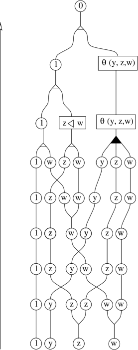
Figure 32: A sample computation with a $3$-cocycle

The result follows. $\Box$

Theorem 7.5

For the cocycles in Theorem 7.4, the following holds: If $\theta$ is not a coboundary, then $\hat{\theta}$ is not a coboundary. In particular, if $H^{3}_{\rm Q}(X;k)\neq 0$, then $H^{3,1}_{\rm sh}(W;W)\neq 0$.

Proof. The proof is similar to that of Theorem 7.3. The cochain $\theta$ is a coboundary if and only if there is a $2$-cochain $\phi$ such that $\delta\phi=\theta$, which is written as $\theta(x,y,z)=\phi(x,y)+\phi(x\triangleleft y,z)-\phi(x,z)-\phi(x\triangleleft z,y\triangleleft z)$ for any $x,y,z\in X$ (see [10]).

Suppose $\hat{\theta}$ is a coboundary. Then there is a $2$-cochain $f$ such that $D_{2}(f)=\hat{\theta}$. A $2$-cochain $f$, in this case, is a map $f:W\otimes W\rightarrow W(=k\oplus kX)$, that is written as:

$$f(\ (a+\sum a_{x}x)\otimes(b+\sum b_{y}y)\ )=f_{0}(\ (a+\sum a_{x}x)\otimes(b+\sum b_{y}y)\ )+f_{1}(\ (a+\sum a_{x}x)\otimes(b+\sum b_{y}y)\ ),$$

where $a\in k$, $x,y\in X$, $f_{0}(a+\sum a_{x}x)\in k$, and $f_{1}(a+\sum a_{x}x)\in kX$. We take specific values and compute $\hat{\theta}=D_{2}(f)$ evaluated at $x\otimes y\otimes z$. We have $\hat{\theta}(x\otimes y\otimes z)=\theta(x,y,z)$, and

$$D_{2}(f)(x\otimes y\otimes z) = [\ f_{0}(x\otimes y)+f_{1}(x\otimes y)\triangleleft z+f_{0}((x\triangleleft y)\otimes z)+f_{1}((x\triangleleft y)\otimes z)\ ]$$

$$- [\ f_{0}((x\triangleleft z)\otimes(y\triangleleft z))+f_{1}((x\triangleleft z)\otimes(y\triangleleft z))+f_{0}(x\otimes z)$$

$$+f_{1}(x\otimes z)\triangleleft(y\triangleleft z)+(x\triangleleft z)\triangleleft f_{1}(y\otimes z)\ ],$$

and comparing the elements on $k$, we obtain

$$\theta(x,y,z)=f_{0}(x\otimes y)+f_{0}((x\triangleleft y)\otimes z)-f_{0}((x\triangleleft z)\otimes(y\triangleleft z))-f_{0}(x\otimes z),$$

so that by defining $\phi(x,y)=f_{0}(x\otimes y)$ for any $x,y\in X$, we obtain a contradiction $\theta=\delta\phi$. $\Box$

7.2 Lie Algebra Cohomology

Let $q:N\otimes N\rightarrow N$ be the map defined in Lemma 3.2, where $N=k\oplus{\mathfrak{g}}$ for a Lie algebra ${\mathfrak{g}}$ over a ground field $k$. Let $\psi:{\mathfrak{g}}\times{\mathfrak{g}}\rightarrow{\mathfrak{g}}$ be a Lie algebra $2$-cocycle, with adjoint action. Then $\psi$ is bilinear and satisfies

$$\psi(y,x)=-\psi(x,y),$$

$$[\psi(x,y),z]+[\psi(y,z),x]+[\psi(z,x),y]+\psi([x,y],z)+\psi([y,z],x)+\psi([z,x],y)=0.$$

It defines a linear map $\psi:{\mathfrak{g}}\otimes{\mathfrak{g}}\rightarrow{\mathfrak{g}}$. The following result says that a Lie algebra $2$-cocycle gives rise to a shelf $2$-cocycle, when the comultiplication is fixed and undeformed ($\eta_{2}=0$).

Theorem 7.6

Let $\psi:{\mathfrak{g}}\times{\mathfrak{g}}\rightarrow{\mathfrak{g}}$ be a Lie algebra $2$-cocycle with adjoint action. Define $\hat{\psi}:N\otimes N\rightarrow N$ by $\hat{\psi}((a+x)\otimes(b+y))=\psi(x\otimes y)$ for $a,b,c\in k$, $x,y,z\in{\mathfrak{g}}$. Then $\hat{\psi}$ is a shelf $2$-cocycle: $d^{2,1}(\hat{\psi},0)=d^{2,2}(\hat{\psi},0)=0.$

Proof. One computes:

$$d^{2,1}(\hat{\psi},0)(\ (a+x)\otimes(b+y)\otimes(c+z)\ )$$

$$= \{\ q(\ \psi(x,y)\otimes(c+z)\ )+\hat{\psi}(\ (ab+bx+[x,y])\otimes(c+z)\ )\}$$

$$- \{\ \{\ \hat{\psi}(q\otimes q)+q(\hat{\psi}\otimes q)+q(q\otimes\hat{\psi})\ \}\tau_{2}(\ (a+x)\otimes(b+y)\otimes(\ (c+z)\otimes 1+1\otimes z\ )\ )\ \}$$

$$= \{\ (c\psi(x,y)+[\psi(x,y),z]\ )+(\ b\psi(x,z)+\psi([x,y],z)\ )\ \}$$

$$- \{\ (\ c\psi(x,y)+\psi([x,z],y)+\psi(x,[y,z])\ )$$

$$+(\ b\psi(x,z)+[\psi(x,z),y]\ )+(\ [x,\psi(y,z)]\ )\ \}\quad=0.$$

The other equality $d^{2,2}(\hat{\psi},0)=0$ is checked similarly. $\Box$

Next we consider Lie algebra $2$-cocycles $\psi:{\mathfrak{g}}\times{\mathfrak{g}}\rightarrow k$ with the trivial representation on the ground field $k$. In this case the $2$-cocycle condition is being skew-symmetric and satisfying the Jacobi identity:

$$\psi(y,x) = -\psi(x,y),$$

$$\psi([x,y],z)+\psi([y,z],x)+\psi([z,x],y) = 0.$$

Let ${\mathfrak{g}}^{\prime}=k\gamma+{\mathfrak{g}}$ where $\gamma\in{\mathfrak{g}}$ and $[\gamma,z]=0$ for all $z\in{\mathfrak{g}}$. Then ${\mathfrak{g}}^{\prime}$ is a Lie algebra with Lie bracket given by $[a\gamma+x,b\gamma+y]^{\prime}=[x,y]\in{\mathfrak{g}}\subset{\mathfrak{g}}^{\prime}$. For a given $2$-cocycle $\psi:{\mathfrak{g}}\times{\mathfrak{g}}\rightarrow k$, define $\psi^{\prime}:{\mathfrak{g}}^{\prime}\times{\mathfrak{g}}^{\prime}\rightarrow{\mathfrak{g}}^{\prime}$ by $\psi^{\prime}(a\gamma+x,b\gamma+y)=\psi(x,y)\gamma\in{\mathfrak{g}}^{\prime}$. Then we claim that $\psi^{\prime}$ satisfies the $2$-cocycle condition with adjoint action. We compute:

$$[\psi^{\prime}(a\gamma+x,b\gamma+y),c\gamma+z]^{\prime}=[\psi(x,y)\gamma,c\gamma+z]^{\prime}=[\psi(x,y)\gamma,z]=0.$$

Therefore the first three terms involving the adjoint action, in fact, vanish by construction. The last three terms reduce to the $2$-cocycle condition of $\psi$, since

$$\psi^{\prime}([a\gamma+x,b\gamma+y]^{\prime},c\gamma+z)=\psi^{\prime}([x,y],c\gamma+z)=\psi([x,y],z).$$

Hence this reduces to the previous case. We summarize this situation as:

Theorem 7.7

A Lie algebra $2$-cocycle valued in the ground field with trivial representation gives rise to a shelf $2$-cocycle.

Next we investigate relations for $3$-cocycles. A Lie algebra $3$-cocycle with adjoint action is a totally skew-symmetric trilinear map $\zeta:{\mathfrak{g}}\times{\mathfrak{g}}\times{\mathfrak{g}}\rightarrow{\mathfrak{g}}$ for a Lie algebra ${\mathfrak{g}}$ that satisfies

$$[\zeta(x,y,z),w]-[\zeta(x,y,w),z]+[\zeta(x,z,w),y]-[\zeta(y,z,w),x]$$

$$-\ \zeta([x,y],z,w)+\zeta([x,z],y,w)-\zeta([x,w],y,z)$$

$$+\ \zeta([y,z],x,w)-\zeta([y,w],x,z)+\zeta([z,w],x,y) = 0.$$

This defines a linear map $\zeta:{\mathfrak{g}}\otimes{\mathfrak{g}}\otimes{\mathfrak{g}}\rightarrow{\mathfrak{g}}$. Recall that we defined $N=k\oplus{\mathfrak{g}}$.

Theorem 7.8

Let $\zeta:{\mathfrak{g}}\times{\mathfrak{g}}\times{\mathfrak{g}}\rightarrow{\mathfrak{g}}$ be a Lie algebra $3$-cocycle with adjoint action. Define $\hat{\zeta}:N\otimes N\otimes N\rightarrow N$ by $\hat{\zeta}((a+x)\otimes(b+y)\otimes(c+z))=\zeta(x\otimes y\otimes z)$. Then $\hat{\zeta}$ satisfies $d^{3,1}(\hat{\zeta},0,0)=0$.

Proof. There are four positive ($L_{1},L_{2},L_{3},L_{4}$) and three negative ($R_{1},R_{2},R_{3}$) terms in $d^{3,1}(\hat{\zeta},0,0)$ (the last negative term vanishes because $\xi_{2}=0$ in $(\xi_{1},\xi_{2},\xi_{3})=(\hat{\zeta},0,0)$). We evaluate each term for a general element

$$(a+x)\otimes(b+y)\otimes(c+z)\otimes(d+w)$$

as before. The first term $L_{1}$ is

$$q(\ \zeta(x,y,z)\otimes(d+w)\ )=d\ \zeta(x,y,z)+[\zeta(x,y,z),w].$$

The second term $L_{2}$ is

$$\hat{\zeta}(q\otimes q\otimes 1)(\ (a+x)\otimes\{(c+z)\otimes(b+y)\otimes 1+1\otimes(b+y)\otimes z\}\otimes w\ )$$

$$= \hat{\zeta}(\ (ac+cx+[x,z])\otimes(b+y)\otimes w+(a+x)\otimes[y,z]\otimes w\ )$$

$$= c\ \zeta(x,y,w)+\zeta([x,z],y,w)+\zeta(x,[y,z],w)$$

By similar calculations the remaining terms give

$$L_{3} : b\ \zeta(x,z,w)+[\zeta(x,z,w),y]$$

$$L_{4} : [x,\zeta(y,z,w)]$$

$$R_{1} : b\ \zeta(x,z,w)+\zeta([x,y],z,w)$$

$$R_{2} : c\ \zeta(x,y,w)+[\zeta(x,y,w),z]$$

$$R_{3} : d\ \zeta(x,y,z)+\zeta([x,w],y,z)+\zeta(x,[y,w],z)+\zeta(x,y,[z,w])$$

and the result $(L_{1}+L_{2}+L_{3}+L_{4})-(R_{1}+R_{2}+R_{3})=0$ follows. $\Box$

Theorem 7.9

For the cocycles in Theorem 7.7, the following holds: If $\psi$ is not a coboundary, then $\hat{\psi}$ is not a coboundary. In particular, if the second cohomology group of the Lie algebra cohomology with adjoint action is non-trivial $(H^{2}_{\rm Lie}({\mathfrak{g}};{\mathfrak{g}})\neq 0)$, then $H^{2}_{\rm sh}(N;N)\neq 0$.

Proof. The proof is similar to that of Theorem 7.3. If $\psi$ is a coboundary, then there is a $1$-cochain $g$ such that $\delta g=\psi$, which is written as $\psi(x,y)=[x,g(y)]+[g(x),y]-g([x,y])$ for any $x,y\in{\mathfrak{g}}$.

Suppose $\hat{\phi}$ is a coboundary, then there is a $1$-cochain $f$ such that $D_{1}(f)=\hat{\psi}$. A $1$-cochain $f$, in this case, is a linear map $f:N\rightarrow N(=k\oplus{\mathfrak{g}})$, that is written as $f(a+x)=f_{0}(a+x)+f_{1}(a+x)$, where $a\in k$, $x\in{\mathfrak{g}}$, $f_{0}(a+x)\in k$, and $f_{1}(a+x)\in{\mathfrak{g}}$. The condition $D_{1}(f)=\hat{\phi}$, then, is written as

$$\hat{\psi}(\ (a+x)\otimes(b+y)\ )=\psi(x,y)$$

$$= D_{1}(f)(\ (a+x)\otimes(b+y)\ )$$

$$= \{q(1\otimes f)-fq+q(f\otimes 1)\}(\ (a+x)\otimes(b+y)\ )$$

In particular, for $(a+x,b+y)=(x,y)$, we obtain

$$\psi(x,y) = q(x\otimes f_{1}(y))-(f_{0}(q(x\otimes y))+f_{1}(q(x\otimes y)))+(f_{0}(x)+q(f_{1}(x)\otimes y))$$

$$= [x,f_{1}(y)]-f_{0}([x,y])-f_{1}([x,y])+f_{0}(x)+[f_{1}(x),y].$$

Comparing the elements in $k$ and ${\mathfrak{g}}$ in the image, we obtain

$$0 = -f_{0}([x,y])+f_{0}(x),$$

$$\psi(x,y) = [x,f_{1}(y)]-f_{1}([x,y])+[f_{1}(x),y],$$

and the second implies that $\psi$ is a coboundary. $\Box$

Let $W_{p}$ be the Witt algebra, a Lie algebra over the field ${\mathbb{F}}_{p}$ with $p$ elements for a prime $p>3$. Specifically, $W_{p}$ has basis $e_{a}$, $a\in{\mathbb{F}}_{p}$ and has bracket defined by $[e_{a},e_{b}]=(b-a)e_{a+b}$. Then it is known [5] (we thank J. Feldvoss for informing us) that the Lie algebra cohomology with trivial action $H^{2}_{\rm Lie}(W_{p};{\mathbb{F}}_{p})$ is one-dimensional and generated by the Virasoro cocycle $c(e_{a},e_{-a})=a(a^{2}-1)$ (otherwise zero). Let $W_{p}^{\prime}=k\gamma\oplus W_{p}$, $N(W_{p}^{\prime})=k\oplus W_{p}^{\prime}$ be the object in ${\rm CoComCoalg}$ with a self-distributive linear map $q$ constructed in Section 3.1. Then we have:

Corollary 7.10

$H^{2}_{\rm sh}(N(W_{p}^{\prime});N(W_{p}^{\prime}))\neq 0$.

8 A Compendium of Questions

What are more precise relationships among the Lie bracket, self-distributivity, solutions to the Yang-Baxter equations, Hopf algebras, and quantum groups? Can the cocycles constructed herein be used to construct invariants of knots and knotted surfaces? Can the coboundary maps be expressed skein theoretically? Is there a spectral sequence that is associated to a filtration of the chain groups? If so, what are the differentials? What does it compute? Are there non-trivial cocycles among any of the trigonometric shelves? The proofs of the main theorems come from grinding through computation. Are there more conceptual proofs? How can the theory be extended to higher dimensions, such as to higher dimensional Lie algebras, or Lie $2$-algebras? How, if at all, do the Zamolodchikov tetrahedron equation and the Jacobiator identity of a Lie $2$-algebra, relate to shelf cohomology? Can it be shown to be a cohomology theory in the case when $\xi_{2}$ and $\xi_{3}$ are non-zero? Is there a spin-foam interpretation of the $3$-cocycle conditions?

Appendix A Proving $D_{3}D_{2}=0$

The next illustrations represent the proofs of Lemmas 6.3 and 6.4.

Figure 33: $d^{3,1}d^{2,1}(\eta_{1},0)$, LHS

Figure 34: $d^{3,1}d^{2,1}(\eta_{1},0)$, RHS

Figure 35: $d^{3,2}d^{2,1}(\eta_{1},0)$, LHS

Figure 36: $d^{3,2}d^{2,1}(\eta_{1},0)$, RHS

Figure 37: $d^{3,3}d^{2,1}(\eta_{1},0)=0$

Appendix B Proving identities between terms in Fig. 33 and 34

The next illustrations give the outlines of the proofs that the terms labelled $7$, $10$, $11$, $12$, $13$, and $14$ represent the same functions in Figs. 33 and 34.

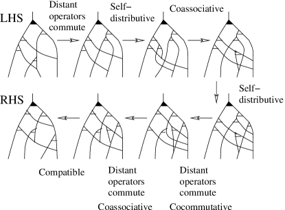
Figure 38: The term $7$

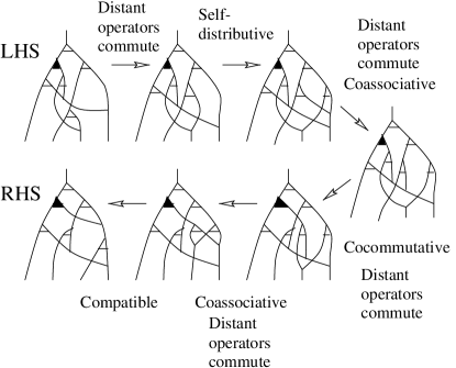
Figure 39: The term $10$

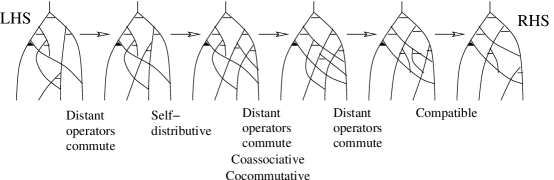
Figure 40: The term $11$

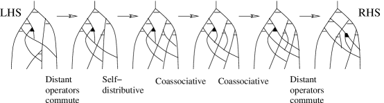
Figure 41: The term $12$

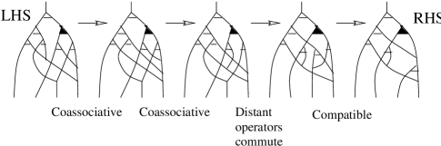
Figure 42: The term $13$

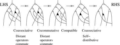
Figure 43: The term $14$

References

- [1] Andruskiewitsch, N.; Graña, M., From racks to pointed Hopf algebras, Adv. in Math. 178 (2003), 177–243.
- [2] Baez, J.C.; Crans, A.S., Higher-Dimensional Algebra VI: Lie 2-Algebras, Theory and Applications of Categories 12 (2004), 492–538.
- [3] Baez, J.C.; Langford, L., -tangles, Lett. Math. Phys. 43 (1998), 187–197.
- [4] Birman, J., Braids, Links, and Mapping Class Groups, Princeton U. Press, Princeton, 1974.
- [5] Block, R. E., On the extensions of Lie algebras Canad. J. Math. 20 (1968), 1439-1450.
- [6] Brieskorn, E., Automorphic sets and singularities, Contemporary math. 78 (1988), 45–115.
- [7] G. Burde and H. Zieschang, Knots, Walter de Gruyter, New York, 1985.
- [8] Carter, J.S.; Elhamdadi, M.; Saito, M., Twisted Quandle homology theory and cocycle knot invariants Algebraic and Geometric Topology (2002) 95–135.
- [9] Carter, J.S.; Elhamdadi, M.; Saito, M., Homology theory for the set-theoretic Yang?Baxter equation and knot invariants from generalizations of quandles, Fund. Math. 184 (2004), 31-54.
- [10] Carter, J.S.; Jelsovsky, D.; Kamada, S.; Langford, L.; Saito, M., Quandle cohomology and state-sum invariants of knotted curves and surfaces, Trans. Amer. Math. Soc. 355 (2003), no. 10, 3947–3989.
- [11] Carter, J.S.; Kamada, S.; Saito, M., “Surfaces in 4-space.” Encyclopaedia of Mathematical Sciences, 142. Low-Dimensional Topology, III. Springer-Verlag, Berlin, 2004.
- [12] Crans, A.S., Lie -algebras, Ph.D. Dissertation, 2004, UC Riverside, available at arXive:math.QA/0409602.
- [13] Ehresmann, C., Categories structurees, Ann. Ec. Normale Sup. 80 (1963). Ehresmann, C., Categories structurees III: Quintettes et applications covariantes, Cahiers Top. et GD V (1963). Ehresmann, C., Introduction to the theory of structured categories, Technical Report Univ. of Kansas at Lawrence (1966).
- [14] Fenn, R.; Rourke, C., Racks and links in codimension two, Journal of Knot Theory and Its Ramifications Vol. 1 No. 4 (1992), 343–406.
- [15] Hennings, M.A., On solutions to the braid equation identified by Woronowicz, Lett. Math. Phys. 27 (1993), 13–17.
- [16] Joyce, D., A classifying invariant of knots, the knot quandle, J. Pure Appl. Alg. 23, 37–65.
- [17] Kauffman, L.H., Knots and Physics, World Scientific, Series on knots and everything, vol. 1, 1991.
- [18] Kuperberg, G. Involutory Hopf algebras and -manifold invariants. Internat. J. Math. 2 (1991), no. 1, 41–66.
- [19] Majid, S. “A quantum groups primer.” London Mathematical Society Lecture Note Series, 292. Cambridge University Press, Cambridge, 2002.
- [20] Majid, S. “Foundations of quantum group theory.” Cambridge University Press, Cambridge, 1995.
- [21] Markl, M., Lie elements in pre-Lie algebras, trees and cohomology operations, Preprint, arXiv:math.AT/0509293.
- [22] Markl, M.; Stasheff, J.D., Deformation theory via deviations, J. Algebra 170 (1994), 122–155.
- [23] Matveev, S., Distributive groupoids in knot theory, (Russian) Mat. Sb. (N.S.) 119(161) (1982), no. 1, 78–88, 160.
- [24] Mochizuki, T., Some calculations of cohomology groups of finite Alexander quandles, J. Pure Appl. Algebra 179 (2003), 287–330.
- [25] Takasaki, M., Abstraction of symmetric Transformations: Introduction to the Theory of kei, T?hoku Math. J. 49, (1943). 145–207 ( a recent translation by Seiichi Kamada is available from that author).
- [26] Woronowicz, S.L., Solutions of the braid equation related to a Hopf algebra, Lett. Math. Phys. 23 (1991), 143–145.
- [27] Yetter, D. N. “Functorial knot theory. Categories of tangles, coherence, categorical deformations, and topological invariants.” Series on Knots and Everything, 26. World Scientific Publishing Co., Inc., River Edge, NJ, 2001.