Erlangen Program at Large—0: Starting with the Group $SL_{2}{}(\mathbb{R}{})$

The simplest objects with non-commutative multiplication may be $2\times 2$ matrices with real entries. Such matrices of determinant one form a closed set under multiplication (since $\det(AB)=\det A\cdot\det B$), the identity matrix is among them and any such matrix has an inverse (since $\det A\neq 0$). In other words those matrices form a group, the $SL_{2}{}(\mathbb{R}{})$ group [Lang85]—one of the two most important Lie groups in analysis. The other group is the Heisenberg group [Howe80a]. By contrast the “$ax+b$”-group, which is often used to build wavelets, is only a subgroup of $SL_{2}{}(\mathbb{R}{})$, see the numerator in (1).

The simplest non-linear transforms of the real line—linear-fractional or Möbius maps—may also be associated with $2\times 2$ matrices [Beardon05a]*Ch. 13:

(1) $$g:x\mapsto g\cdot x=\frac{ax+b}{cx+d},\text{ where }g=\begin{pmatrix}a&b\\ c&d\end{pmatrix},x\in\mathbb{R}{}.$$

An enjoyable calculation shows that the composition of two transforms (1) with different matrices $g_{1}$ and $g_{2}$ is again a Möbius transform with matrix the product $g_{1}g_{2}$. In other words (1) it is a (left) action of $SL_{2}{}(\mathbb{R}{})$.

According to F. Klein’s Erlangen program (which was influenced by S. Lie) any geometry is dealing with invariant properties under a certain group action. For example, we may ask: What kinds of geometry are related to the $SL_{2}{}(\mathbb{R}{})$ action (1)?

The Erlangen program has probably the highest rate of $\frac{\text{praised}}{\text{actually used}}$ among mathematical theories not only due to the big numerator but also due to undeserving small denominator. As we shall see below Klein’s approach provides some surprising conclusions even for such over-studied objects as circles.

1. Make a Guess in Three Attempts

It is easy to see that the $SL_{2}{}(\mathbb{R}{})$ action (1) makes sense also as a map of complex numbers $z=x+\mathrm{i}y$, $\mathrm{i}^{2}=-1$. Moreover, if $y>0$ then $g\cdot z$ has a positive imaginary part as well, i.e. (1) defines a map from the upper half-plane to itself.

However there is no need to be restricted to the traditional route of complex numbers only. Less-known dual and double numbers [Yaglom79]*Suppl. C have also the form $z=x+\mathrm{i}y$ but different assumptions on the imaginary unit $\mathrm{i}$: $\mathrm{i}^{2}=0$ or $\mathrm{i}^{2}=1$ correspondingly. Although the arithmetic of dual and double numbers is different from the complex ones, e.g. they have divisors of zero, we are still able to define their transforms by (1) in most cases.

Three possible values $-1$, $0$ and $1$ of $\sigma:=\mathrm{i}^{2}$ will be refereed to here as elliptic, parabolic and hyperbolic cases respectively. We repeatedly meet such a division of various mathematical objects into three classes. They are named by the historically first example—the classification of conic sections—however the pattern persistently reproduces itself in many different areas: equations, quadratic forms, metrics, manifolds, operators, etc. We will abbreviate this separation as EPH-classification. The common origin of this fundamental division can be seen from the simple picture of a coordinate line split by zero into negative and positive half-axes:

(2)

Connections between different objects admitting EPH-classification are not limited to this common source. There are many deep results linking, for example, ellipticity of quadratic forms, metrics and operators. On the other hand there are still a lot of white spots and obscure gaps between some subjects as well.

To understand the action (1) in all EPH cases we use the Iwasawa decomposition [Lang85] of $SL_{2}{}(\mathbb{R}{})=ANK$ into three one-dimensional subgroups $A$, $N$ and $K$:

(3) $$\begin{pmatrix}a&b\\ c&d\end{pmatrix}={\begin{pmatrix}\alpha&0\\ 0&\alpha^{-1}\end{pmatrix}}{\begin{pmatrix}1&\nu\\ 0&1\end{pmatrix}}{\begin{pmatrix}\cos\phi&\sin\phi\\ -\sin\phi&\cos\phi\end{pmatrix}}.$$

Subgroups $A$ and $N$ act in (1) irrespectively to value of $\sigma$: $A$ makes a dilation by $\alpha^{2}$, i.e. $z\mapsto\alpha^{2}z$, and $N$ shifts points to left by $\nu$, i.e. $z\mapsto z+\nu$.

By contrast, the action of the third matrix from the subgroup $K$ sharply depends on $\sigma$, see Fig. 1. In elliptic, parabolic and hyperbolic cases $K$-orbits are circles, parabolas and (equilateral) hyperbolas correspondingly. Thin traversal lines in Fig. 1 join points of orbits for the same values of $\phi$ and grey arrows represent “local velocities”—vector fields of derived representations.

Definition 1.

The common name cycle [Yaglom79] is used to denote circles, parabolas and hyperbolas (as well as straight lines as their limits) in the respective EPH case.

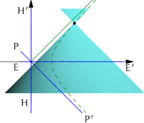
(a)                  (b)

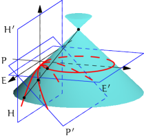
Figure 2. $K$-orbits as conic sections: circles are sections by the plane $EE^{\prime}$; parabolas are sections by $PP^{\prime}$; hyperbolas are sections by $HH^{\prime}$. Points on the same generator of the cone correspond to the same value of $\phi$.

It is well known that any cycle is a conic sections and an interesting observation is that corresponding $K$-orbits are in fact sections of the same two-sided right-angle cone, see Fig. 2. Moreover, each straight line generating the cone, see Fig. 2(b), is crossing corresponding EPH $K$-orbits at points with the same value of parameter $\phi$ from (3). In other words, all three types of orbits are generated by the rotations of this generator along the cone.

$K$-orbits are $K$-invariant in a trivial way. Moreover since actions of both $A$ and $N$ for any $\sigma$ are extremely “shape-preserving” we find natural invariant objects of the Möbius map:

Theorem 2.

The family of all cycles from Defn. 1 is invariant under the action (1).

Proof.

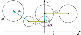
Figure 3. Decomposition of an arbitrary Möbius transformation $g$ into a product $g=g_{a}g_{n}g_{k}g_{a}^{\prime}g_{n}^{\prime}$.

We will show that for a given $g\in SL_{2}{}(\mathbb{R}{})$ and a cycle $C$ its image $gC$ is again a cycle. Fig. 3 make an illustration with $C$ as a circle, but our reasoning works in all EPH cases.

For a fixed $C$ there is always the unique pair of transformations $g^{\prime}_{n}$ from the subgroup $N$ and $g^{\prime}_{a}\in A$ that the cycle $g^{\prime}_{a}g^{\prime}_{n}C$ is exactly a $K$-orbit. We make a decomposition of $g(g^{\prime}_{a}g^{\prime}_{n})^{-1}$ into a product as in (3):

$$g(g^{\prime}_{a}g^{\prime}_{n})^{-1}=g_{a}g_{n}g_{k}.$$

Since $g^{\prime}_{a}g^{\prime}_{n}C$ is a $K$-orbit we have $g_{k}(g^{\prime}_{a}g^{\prime}_{n}C)=g^{\prime}_{a}g^{\prime}_{n}C$, then:

$$gC = g(g^{\prime}_{a}g^{\prime}_{n})^{-1}g^{\prime}_{a}g^{\prime}_{n}C=g_{a}g_{n}g_{k}g^{\prime}_{a}g^{\prime}_{n}C$$

$$= g_{a}g_{n}g_{k}(g^{\prime}_{a}g^{\prime}_{n}C)=g_{a}g_{n}g^{\prime}_{a}g^{\prime}_{n}C,$$

Since subgroups $A$ and $N$ obviously preserve the shape of any cycle this finishes our proof. ∎

According to Erlangen ideology we should now study invariant properties of cycles.

2. Invariance of FSCc

Fig. 2 suggests that we may get a unified treatment of cycles in all EPH by consideration of a higher dimension spaces. The standard mathematical method is to declare objects under investigations (cycles in our case, functions in functional analysis, etc.) to be simply points of some bigger space. This space should be equipped with an appropriate structure to hold externally information which were previously inner properties of our objects.

A generic cycle is the set of points $(u,v)\in\mathbb{R}^{2}{}$ defined for all values of $\sigma$ by the equation

(4) $$k(u^{2}-\sigma v^{2})-2lu-2nv+m=0.$$

This equation (and the corresponding cycle) is defined by a point $(k,l,n,m)$ from a projective space $\mathbb{P}^{3}{}$, since for a scaling factor $\lambda\neq 0$ the point $(\lambda k,\lambda l,\lambda n,\lambda m)$ defines the same equation (4). We call $\mathbb{P}^{3}{}$ the cycle space and refer to the initial $\mathbb{R}^{2}{}$ as the point space.

In order to get a connection with Möbius action (1) we arrange numbers $(k,l,n,m)$ into the matrix

(5) $$C_{\breve{\sigma}}^{s}=\begin{pmatrix}l+\mathrm{\breve{\i}}sn&-m\\ k&-l+\mathrm{\breve{\i}}sn\end{pmatrix},$$

with a new imaginary unit $\mathrm{\breve{\i}}$ and an additional parameter $s$ usually equal to $\pm 1$. The values of $\breve{\sigma}:=\mathrm{\breve{\i}}^{2}$ is $-1$, $0$ or $1$ independently from the value of $\sigma$. The matrix (5) is the cornerstone of (extended) Fillmore–Springer–Cnops construction (FSCc) [Cnops02a] and closely related to technique recently used by A.A. Kirillov to study the Apollonian gasket [Kirillov06].

The significance of FSCc in Erlangen framework is provided by the following result:

Theorem 3.

The image $\tilde{C}_{\breve{\sigma}}^{s}$ of a cycle $C_{\breve{\sigma}}^{s}$ under transformation (1) with $g\in SL_{2}{}(\mathbb{R}{})$ is given by similarity of the matrix (5):

(6) $$\tilde{C}_{\breve{\sigma}}^{s}=gC_{\breve{\sigma}}^{s}g^{-1}.$$

In other words FSCc (5) intertwines Möbius action (1) on cycles with linear map (6).

There are several ways to prove (6): either by a brute force calculation (fortunately performed by a CAS) [Kisil05a] or through the related orthogonality of cycles [Cnops02a], see the end of the next section 3.

The important observation here is that FSCc (5) uses an imaginary unit $\mathrm{\breve{\i}}$ which is not related to $\mathrm{i}$ defining the appearance of cycles on plane. In other words any EPH type of geometry in the cycle space $\mathbb{P}^{3}{}$ admits drawing of cycles in the point space $\mathbb{R}^{2}{}$ as circles, parabolas or hyperbolas. We may think on points of $\mathbb{P}^{3}{}$ as ideal cycles while their depictions on $\mathbb{R}^{2}{}$ are only their shadows on the wall of Plato’s cave.

Fig. 4(a) shows the same cycles drawn in different EPH styles. Points $c_{e,p,h}=(\frac{l}{k},-\sigma\frac{n}{k})$ are their respective e/p/h-centres. They are related to each other through several identities:

(7) $$c_{e}=\bar{c}_{h},\quad c_{p}=\frac{1}{2}(c_{e}+c_{h}).$$

Fig. 4(b) presents two cycles drawn as parabolas, they have the same focal length $\frac{n}{2k}$ and thus their e-centres are on the same level. In other words concentric parabolas are obtained by a vertical shift, not scaling as an analogy with circles or hyperbolas may suggest.

Fig. 4(b) also presents points, called e/p/h-foci:

(8) $$f_{e,p,h}=\left(\frac{l}{k},-\frac{\det C_{\breve{\sigma}}^{s}}{2nk}\right),$$

which are independent of the sign of $s$. If a cycle is depicted as a parabola then h-focus, p-focus, e-focus are correspondingly geometrical focus of the parabola, its vertex, and the point on the directrix nearest to the vertex.

As we will see, cf. Thms. 5 and 7, all three centres and three foci are useful attributes of a cycle even if it is drawn as a circle.

3. Invariants: algebraic and geometric

We use known algebraic invariants of matrices to build appropriate geometric invariants of cycles. It is yet another demonstration that any division of mathematics into subjects is only illusive.

For $2\times 2$ matrices (and thus cycles) there are only two essentially different invariants under similarity (6) (and thus under Möbius action (1)): the trace and the determinant. The latter was already used in (8) to define cycle’s foci. However due to projective nature of the cycle space $\mathbb{P}^{3}{}$ the absolute values of trace or determinant are irrelevant, unless they are zero.

Alternatively we may have a special arrangement for normalisation of quadruples $(k,l,n,m)$. For example, if $k\neq 0$ we may normalise the quadruple to $(1,\frac{l}{k},\frac{n}{k},\frac{m}{k})$ with highlighted cycle’s centre. Moreover in this case $\det{C^{s}_{\breve{\sigma}}}$ is equal to the square of cycle’s radius, cf. Section 6. Another normalisation $\det{C^{s}_{\breve{\sigma}}}=1$ is used in [Kirillov06] to get a nice condition for touching circles.

We still get important characterisation even with non-normalised cycles, e.g., invariant classes (for different $\breve{\sigma}$) of cycles are defined by the condition $\det C_{\breve{\sigma}}^{s}=0$. Such a class is parametrises only by two real number and as such is easily attached to certain point of $\mathbb{R}^{2}{}$. For example, the cycle $C_{\breve{\sigma}}^{s}$ with $\det C_{\breve{\sigma}}^{s}=0$, $\breve{\sigma}=-1$ drawn elliptically represent just a point $(\frac{l}{k},\frac{n}{k})$, i.e. (elliptic) zero-radius circle. The same condition with $\breve{\sigma}=1$ in hyperbolic drawing produces a null-cone originated at point $(\frac{l}{k},\frac{n}{k})$:

$$(u-\frac{l}{k})^{2}-(v-\frac{n}{k})^{2}=0,$$

i.e. a zero-radius cycle in hyperbolic metric.

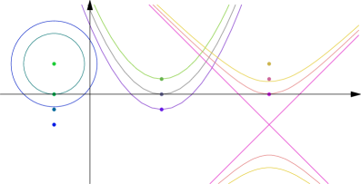
Figure 5. Different $\mathrm{i}$-implementations of the same $\breve{\sigma}$-zero-radius cycles and corresponding foci.

In general for every notion there is nine possibilities: three EPH cases in the cycle space times three EPH realisations in the point space. Such nine cases for “zero radius” cycles is shown on Fig. 5. For example, p-zero-radius cycles in any implementation touch the real axis.

This “touching” property is a manifestation of the boundary effect in the upper-half plane geometry [Kisil05a]*Rem. 3.4. The famous question on hearing drum’s shape has a sister:

Can we see/feel the boundary from inside a domain?

Both orthogonality relations described below are “boundary aware” as well. It is not surprising after all since $SL_{2}{}(\mathbb{R}{})$ action on the upper-half plane was obtained as an extension of its action (1) on the boundary.

According to the categorical viewpoint internal properties of objects are of minor importance in comparison to their relations with other objects from the same class. As an illustration we may put the proof of Thm. 3 sketched at the end of of the next section. Thus from now on we will look for invariant relations between two or more cycles.

4. Joint invariants: orthogonality

The most expected relation between cycles is based on the following Möbius invariant “inner product” build from a trace of product of two cycles as matrices:

(9) $$\left\langle C_{\breve{\sigma}}^{s},\tilde{C}_{\breve{\sigma}}^{s}\right\rangle=\mathop{tr}(C_{\breve{\sigma}}^{s}\tilde{C}_{\breve{\sigma}}^{s})$$

By the way, an inner product of this type is used, for example, in GNS construction to make a Hilbert space out of $C^{*}$-algebra. The next standard move is given by the following definition.

Definition 4.

Two cycles are called $\breve{\sigma}$-orthogonal if $\left\langle C_{\breve{\sigma}}^{s},\tilde{C}_{\breve{\sigma}}^{s}\right\rangle=0$.

For the case of $\breve{\sigma}\sigma=1$, i.e. when geometries of the cycle and point spaces are both either elliptic or hyperbolic, such an orthogonality is the standard one, defined in terms of angles between tangent lines in the intersection points of two cycles. However in the remaining seven ($=9-2$) cases the innocent-looking Defn. 4 brings unexpected relations.

Elliptic (in the point space) realisations of Defn. 4, i.e. $\sigma=-1$ is shown in Fig. 6. The left picture corresponds to the elliptic cycle space, e.g. $\breve{\sigma}=-1$. The orthogonality between the red circle and any circle from the blue or green families is given in the usual Euclidean sense. The central (parabolic in the cycle space) and the right (hyperbolic) pictures show non-local nature of the orthogonality. There are analogues pictures in parabolic and hyperbolic point spaces as well [Kisil05a].

This orthogonality may still be expressed in the traditional sense if we will associate to the red circle the corresponding “ghost” circle, which shown by the dashed line in Fig. 6. To describe ghost cycle we need the Heaviside function $\chi(\sigma)$:

(10) $$\chi(t)=\left\{\begin{array}[]{ll}1,&t\geq 0;\\ -1,&t<0.\end{array}\right.$$

Theorem 5.

A cycle is $\breve{\sigma}$-orthogonal to cycle $C_{\breve{\sigma}}^{s}$ if it is orthogonal in the usual sense to the $\sigma$-realisation of “ghost” cycle $\hat{C}_{\breve{\sigma}}^{s}$, which is defined by the following two conditions:

1. $\chi(\sigma)$-centre of $\hat{C}_{\breve{\sigma}}^{s}$ coincides with $\breve{\sigma}$-centre of $C_{\breve{\sigma}}^{s}$.

2. Cycles $\hat{C}_{\breve{\sigma}}^{s}$ and $C^{s}_{\breve{\sigma}}$ have the same roots, moreover $\det\hat{C}_{\sigma}^{1}=\det C^{\chi(\breve{\sigma})}_{\sigma}$.

The above connection between various centres of cycles illustrates their meaningfulness within our approach.

One can easy check the following orthogonality properties of the zero-radius cycles defined in the previous section:

1. Since $\left\langle C_{\breve{\sigma}}^{s},{C}_{\breve{\sigma}}^{s}\right\rangle=\det{C}_{\breve{\sigma}}^{s}$ zero-radius cycles are self-orthogonal (isotropic) ones.

2. A cycle ${C^{s}_{\breve{\sigma}}}$ is $\sigma$-orthogonal to a zero-radius cycle $Z^{s}_{\breve{\sigma}}$ if and only if ${C^{s}_{\breve{\sigma}}}$ passes through the $\sigma$-centre of $Z^{s}_{\breve{\sigma}}$.

Sketch of proof of Thm. 3.

The validity of Thm. 3 for a zero-radius cycle

$$Z^{s}_{\breve{\sigma}}=\begin{pmatrix}z&-z\bar{z}\\ 1&-\bar{z}\end{pmatrix}=\frac{1}{2}\begin{pmatrix}z&z\\ 1&1\end{pmatrix}\begin{pmatrix}1&-\bar{z}\\ 1&-\bar{z}\end{pmatrix}$$

with the centre $z=x+\mathrm{i}y$ is straightforward. This implies the result for a generic cycle with the help of Möbius invariance of the product (9) (and thus the orthogonality) and the above relation (ii) between the orthogonality and the incidence. See [Cnops02a] for details. ∎

5. Higher order joint invariants: s-orthogonality

With appetite already wet one may wish to build more joint invariants. Indeed for any homogeneous polynomial $p(x_{1},x_{2},\ldots,x_{n})$ of several non-commuting variables one may define an invariant joint disposition of $n$ cycles ${}^{j}\!{C^{s}_{\breve{\sigma}}}$ by the condition:

$$\mathop{tr}p({}^{1}\!{C^{s}_{\breve{\sigma}}},{}^{2}\!{C^{s}_{\breve{\sigma}}},\ldots,{}^{n}\!{C^{s}_{\breve{\sigma}}})=0.$$

However it is preferable to keep some geometrical meaning of constructed notions.

An interesting observation is that in the matrix similarity of cycles (6) one may replace element $g\in SL_{2}{}(\mathbb{R}{})$ by an arbitrary matrix corresponding to another cycle. More precisely the product ${C^{s}_{\breve{\sigma}}}{\tilde{C}^{s}_{\breve{\sigma}}}{C^{s}_{\breve{\sigma}}}$ is again the matrix of the form (5) and thus may be associated to a cycle. This cycle may be considered as the reflection of ${\tilde{C}^{s}_{\breve{\sigma}}}$ in ${C^{s}_{\breve{\sigma}}}$.

Definition 6.

A cycle ${C^{s}_{\breve{\sigma}}}$ is s-orthogonal to a cycle ${\tilde{C}^{s}_{\breve{\sigma}}}$ if the reflection of ${\tilde{C}^{s}_{\breve{\sigma}}}$ in ${C^{s}_{\breve{\sigma}}}$ is orthogonal (in the sense of Defn. 4) to the real line. Analytically this is defined by:

(11) $$\mathop{tr}({C^{s}_{\breve{\sigma}}}{\tilde{C}^{s}_{\breve{\sigma}}}{C^{s}_{\breve{\sigma}}}R^{s}_{\breve{\sigma}})=0.$$

Due to invariance of all components in the above definition s-orthogonality is a Möbius invariant condition. Clearly this is not a symmetric relation: if ${C^{s}_{\breve{\sigma}}}$ is s-orthogonal to ${\tilde{C}^{s}_{\breve{\sigma}}}$ then ${\tilde{C}^{s}_{\breve{\sigma}}}$ is not necessarily s-orthogonal to ${C^{s}_{\breve{\sigma}}}$.

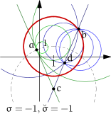
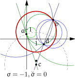
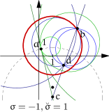
Figure 7. Orthogonality of the second kind for circles. To highlight both similarities and distinctions with the ordinary orthogonality we use the same notations as that in Fig. 6.

Fig. 7 illustrates s-orthogonality in the elliptic point space. By contrast with Fig. 6 it is not a local notion at the intersection points of cycles for all $\breve{\sigma}$. However it may be again clarified in terms of the appropriate s-ghost cycle, cf. Thm. 5.

Theorem 7.

A cycle is s-orthogonal to a cycle $C^{s}_{\breve{\sigma}}$ if its orthogonal in the traditional sense to its s-ghost cycle ${\tilde{C}^{\breve{\sigma}}_{\breve{\sigma}}}={C^{\chi(\sigma)}_{\breve{\sigma}}}\mathbb{R}^{\breve{\sigma}}_{\breve{\sigma}}{}{C^{\chi(\sigma)}_{\breve{\sigma}}}$, which is the reflection of the real line in ${C^{\chi(\sigma)}_{\breve{\sigma}}}$ and $\chi$ is the Heaviside function (10). Moreover

1. $\chi(\sigma)$-Centre of ${\tilde{C}^{\breve{\sigma}}_{\breve{\sigma}}}$ coincides with the $\breve{\sigma}$-focus of ${C^{s}_{\breve{\sigma}}}$, consequently all lines s-orthogonal to ${C^{s}_{\breve{\sigma}}}$ are passing the respective focus.

2. Cycles ${C^{s}_{\breve{\sigma}}}$ and ${\tilde{C}^{\breve{\sigma}}_{\breve{\sigma}}}$ have the same roots.

Note the above intriguing interplay between cycle’s centres and foci. Although s-orthogonality may look exotic it will naturally appear in the end of next Section again.

Of course, it is possible to define another interesting higher order joint invariants of two or even more cycles.

6. Distance, length and perpendicularity

Geometry in the plain meaning of this word deals with distances and lengths. Can we obtain them from cycles?

We mentioned already that for circles normalised by the condition $k=1$ the value $\det{C^{s}_{\breve{\sigma}}}=\left\langle{C^{s}_{\breve{\sigma}}},{C^{s}_{\breve{\sigma}}}\right\rangle$ produces the square of the traditional circle radius. Thus we may keep it as the definition of the radius for any cycle. But then we need to accept that in the parabolic case the radius is the (Euclidean) distance between (real) roots of the parabola, see Fig. 8(a).

Having radii of circles already defined we may use them for other measurements in several different ways. For example, the following variational definition may be used:

Definition 8.

The distance between two points is the extremum of diameters of all cycles passing through both points, see Fig. 8(b).

If $\breve{\sigma}=\sigma$ this definition gives in all EPH cases the distance between endpoints of a vector $z=u+\mathrm{i}v$ as follows:

(12) $$d_{e,p,h}(u,v)^{2}=(u+\mathrm{i}v)(u-\mathrm{i}v)=u^{2}-\sigma v^{2}.$$

The parabolic distance $d_{p}^{2}=u^{2}$, see Fig. 8(b), algebraically sits between $d_{e}$ and $d_{h}$ according to the general principle (2) and is widely accepted [Yaglom79]. However one may be unsatisfied by its degeneracy.

An alternative measurement is motivated by the fact that a circle is the set of equidistant points from its centre. However the choice of “centre” is now rich: it may be either point from three centres (7) or three foci (8).

Definition 9.

The length of a directed interval $\overrightarrow{AB}$ is the radius of the cycle with its centre (denoted by $l_{c}(\overrightarrow{AB})$) or focus (denoted by $l_{f}(\overrightarrow{AB})$) at the point $A$ which passes through $B$.

These definition is less common and have some unusual properties like non-symmetry: $l_{f}(\overrightarrow{AB})\neq l_{f}(\overrightarrow{BA})$. However it comfortably fits the Erlangen program due to its $SL_{2}{}(\mathbb{R}{})$-conformal invariance:

Theorem 10 ([Kisil05a]).

Let $l$ denote either the EPH distances (12) or any length from Defn. 9. Then for fixed $y$, $y^{\prime}\in\mathbb{R}^{\sigma}{}$ the limit:

$$\lim_{t\rightarrow 0}\frac{l(g\cdot y,g\cdot(y+ty^{\prime}))}{l(y,y+ty^{\prime})},\qquad\text{ where }g\in SL_{2}{}(\mathbb{R}{}),$$

exists and its value depends only from $y$ and $g$ and is independent from $y^{\prime}$.

We may return from distances to angles recalling that in the Euclidean space a perpendicular provides the shortest root from a point to a line, see Fig. 8(c).

Definition 11.

Let $l$ be a length or distance. We say that a vector $\overrightarrow{AB}$ is $l$-perpendicular to a vector $\overrightarrow{CD}$ if function $l(\overrightarrow{AB}+\varepsilon\overrightarrow{CD})$ of a variable $\varepsilon$ has a local extremum at $\varepsilon=0$.

A pleasant surprise is that $l_{f}$-perpendicularity obtained thought the length from focus (Defn. 9) coincides with already defined in Section 5 s-orthogonality as follows from Thm. 7(i). It is also possible [Kisil08a] to make $SL_{2}{}(\mathbb{R}{})$ action isometric in all three cases.

All these study are waiting to be generalised to high dimensions and Clifford algebras provide a suitable language for this [Kisil05a, JParker07a].

7. Erlangen program at large

As we already mentioned the division of mathematics into areas is only apparent. Therefore it is unnatural to limit Erlangen program only to “geometry”. We may continue to look for $SL_{2}{}(\mathbb{R}{})$ invariant objects in other related fields. For example, transform (1) generates unitary representations on certain $L_{2}{}$ spaces, cf. (1):

(13) $$g^{-1}:f(x)\mapsto\frac{1}{(cx+d)^{m}}f\left(\frac{ax+b}{cx+d}\right).$$

For $m=1$, $2$, …the invariant subspaces of $L_{2}{}$ are Hardy and (weighted) Bergman spaces of complex analytic functions. All main objects of complex analysis (Cauchy and Bergman integrals, Cauchy-Riemann and Laplace equations, Taylor series etc.) may be obtaining in terms of invariants of the discrete series representations of $SL_{2}{}(\mathbb{R}{})$ [Kisil02c]*§ 3. Moreover two other series (principal and complimentary [Lang85]) play the similar rôles for hyperbolic and parabolic cases [Kisil02c] [Kisil05a].

Moving further we may observe that transform (1) is defined also for an element $x$ in any algebra $\mathfrak{A}$ with a unit $\mathbf{1}$ as soon as $(cx+d\mathbf{1})\in\mathfrak{A}$ has an inverse. If $\mathfrak{A}$ is equipped with a topology, e.g. is a Banach algebra, then we may study a functional calculus for element $x$ [Kisil02a] in this way. It is defined as an intertwining operator between the representation (13) in a space of analytic functions and a similar representation in a left $\mathfrak{A}$-module.

In the spirit of Erlangen program such functional calculus is still a geometry, since it is dealing with invariant properties under a group action. However even for a simplest non-normal operator, e.g. a Jordan block of the length $k$, the obtained space is not like a space of point but is rather a space of $k$-th jets [Kisil02a]. Such non-point behaviour is oftenly attributed to non-commutative geometry and Erlangen program provides an important input on this fashionable topic [Kisil02c].

Of course, there is no reasons to limit Erlangen program to $SL_{2}{}(\mathbb{R}{})$ group only, other groups may be more suitable in different situations. However $SL_{2}{}(\mathbb{R}{})$ still possesses a big unexplored potential and is a good object to start with.

8. Acknowledgements

I am in debt to the Editorial board of the Notices of AMS who spent enormous amount of time correcting and improving this paper. I am also grateful to Prof. Troels Roussau Johansen who pointed out some more misprints and obscure places.

Graphics for this article were created with the help of Open Source Software:

MetaPost (http://www.tug.org/metapost.html),
Asymptote (http://asymptote.sourceforge.net),
and GiNaC (http://www.ginac.de).

Figure 1. Action of the $K$ subgroup. The corresponding $K$-orbits are thick circles, parabolas and hyperbolas. Thin traversal lines are images of the vertical axis for certain values of the parameter $\phi$.

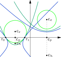
(a)           (b)

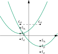
Figure 4. (a) Different EPH implementations of the same cycles defined by quadruples of numbers.
(b) Centres and foci of two parabolas with the same focal length.

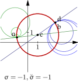
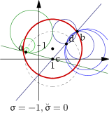
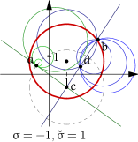
Figure 6. Orthogonality of the first kind in the elliptic point space.
Each picture presents two groups (green and blue) of cycles which are orthogonal to the red cycle $C^{s}_{\breve{\sigma}}$. Point $b$ belongs to $C^{s}_{\breve{\sigma}}$ and the family of blue cycles passing through $b$ is orthogonal to $C^{s}_{\breve{\sigma}}$. They all also intersect in the point $d$ which is the inverse of $b$ in $C^{s}_{\breve{\sigma}}$. Any orthogonality is reduced to the usual orthogonality with a new (“ghost”) cycle (shown by the dashed line), which may or may not coincide with $C^{s}_{\breve{\sigma}}$. For any point $a$ on the “ghost” cycle the orthogonality is reduced to the local notion in the terms of tangent lines at the intersection point. Consequently such a point $a$ is always the inverse of itself.

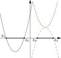
(a) (b) (c)

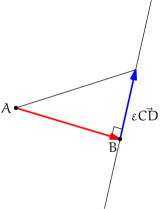
Figure 8. (a) The square of the parabolic diameter is the square of the distance between roots if they are real ($z_{1}$ and $z_{2}$), otherwise the negative square of the distance between the adjoint roots ($z_{3}$ and $z_{4}$).
(b) Distance as extremum of diameters in elliptic ($z_{1}$ and $z_{2}$) and parabolic ($z_{3}$ and $z_{4}$) cases.
(c) Perpendicular as the shortest route to a line.