Abstract.

We present an accessible introduction to basic results on groups of intermediate growth.

Introduction

The study of growth of groups has a long and remarkable history spanning over much of the twentieth century, and goes back to Hilbert, Poincare, Alphors, etc. In 1968 it became apparent that all known classes of groups have either polynomial or exponential growth, and John Milnor formally asked whether groups of intermediate growth exist. The first such examples were introduced by the first author two decades ago [4] (see also [3, 5]), and since then there has been an explosion in the number of works on the subject. While new techniques and application have been developed, much of the literature remains rather specialized, accessible only to specialists in the area. This paper is an attempt to present the material in an introductory manner, to the reader familiar with only basic algebraic concepts.

We concentrate on study of the first construction, a finitely generated group $\mathbb{G}$ introduced by the first author to resolve Milnor’s question, and which became a prototype for further developments. Our Main Theorem shows that $\mathbb{G}$ has intermediate growth, i.e. superpolynomial and subexponential.

Our proof is neither the shortest nor gives the best possible bounds. Instead, we attempt to simplify the presentation as much as possible by breaking the proof into a number of propositions of independent interest, supporting lemmas, and exercises. Along the way we prove two ‘bonus’ theorems: we show that $\mathbb{G}$ is periodic (every element has a finite order) and give a nearly linear time algorithm for the word problem in $\mathbb{G}$. We hope that the beginner readers now have an easy time entering the field and absorbing what is usually viewed as unfriendly material.

Let us warn the reader that this paper neither gives a survey nor presents a new proof of the Main Theorem. We refer to extensive survey articles [1, 2, 6] and a recent book [8] for further results and references. Our proofs roughly follow [5, 10], but the presentation and details are mostly new.

The paper is structured is as follows. We start with some background information on the growth of groups (Section 1) and technical results for bounding the growth function (Section 2). These technical results have elementary analytic nature; their proofs are moved to the Appendix (Section 12). In Section 3 we study the group ${\text{\rm Aut}}(\mathbf{T})$ of automorphisms of an infinite binary (rooted) tree. The ‘first construction’ group $\mathbb{G}$ is introduced in Section 4, while the remaining sections 5–10 prove the intermediate growth of $\mathbb{G}$ and one ‘bonus’ theorem. We conclude with final remarks and few open problems (Section 11).

Notation.  Throughout the paper we use only left group multiplication. For example, a product $\tau_{1}\cdot\tau_{2}$ of automorphisms $\tau_{1},\tau_{2}\in{\text{\rm Aut}}(\mathbf{T})$ is given by $[\tau_{1}\cdot\tau_{2}](v)=\tau_{2}(\tau_{1}(v))$. We use notation $g^{h}=h^{-1}gh$ for conjugate elements, and I for the identity element. Finally, let $\mathbb{N}=\{0,1,2,\ldots\}$.

1. Growth of groups

Let $S=\{s_{1},\ldots,s_{k}\}$ be a generating set of a group $G=\langle S\rangle$. For every group element $g\in G$, denote by $\ell(g)=\ell_{S}(g)$ the length of the shortest decomposition $g\,=\,s_{i_{1}}^{\pm 1}\cdots s_{i_{\ell}}^{\pm 1}$. Let $\gamma_{G}^{S}(n)$ be the number of elements $g\in G$ such that $\ell(g)\leq n$. Function $\gamma=\gamma_{G}^{S}$ is called the growth function of the group $G$ with respect to the generating set $S$. Clearly, $\gamma(n)\,\leq\,\sum_{i=0}^{n}\,(2k)^{n}\,\leq\,(2k+1)^{n}.$

Exercise 1.1.

Let $G$ be an infinite group. Prove that the growth function $\gamma$ is monotone increasing:   $\gamma(n+1)\,>\,\gamma(n)$, for all $n\geq 1$.

Exercise 1.2.

Check that the growth function $\gamma$ is submultiplicative:

$\gamma(m+n)\,\leq\,\gamma(m)\,\gamma(n)$, for all $m,n\geq 1$.

Consider two functions $\gamma,\gamma^{\prime}:\mathbb{N}\to\mathbb{N}$. Define $\gamma\preccurlyeq\gamma^{\prime}$ if $\gamma(n)\leq C\,\gamma^{\prime}(\alpha n)$, for all $n>0$ and some $C,\alpha>0$. We say that $\gamma$ and $\gamma^{\prime}$ are equivalent, write $\gamma\sim\gamma^{\prime}$, if $\gamma\preccurlyeq\gamma^{\prime}$ and $\gamma^{\prime}\preccurlyeq\gamma$.

Exercise 1.3.

Let $S$ and $S^{\prime}$ be two generating sets of $G$. Prove that the corresponding growth functions $\gamma_{G}^{S}$ and $\gamma_{G}^{S^{\prime}}$ are equivalent.

A function $f:\mathbb{N}\to\mathbb{R}$ is called polynomial if $f(n)\sim n^{\alpha}$, for some $\alpha>0$. A function $f$ is called superpolynomial if there exists a limit $\frac{\ln\gamma(n)}{\ln n}\to\infty$ as $n\to\infty$. For example, $n^{\pi}$ is polynomial, while $n^{n}$ and $n^{\log\log n}$ are superpolynomial.

Similarly, a function $f$ is called exponential if $f(n)\sim e^{n}$. A function $f$ is called subexponential if there exists a limit $\frac{\ln\gamma(n)}{n}\to 0$ as $n\to\infty$. For example, $n^{e}e^{n}$ and $\exp\bigl{(}n/2-\sqrt{n}\,\log^{2}n)$ are exponential, $e^{n/\log n}$ and $n^{\pi}$ are subexponential, while $n^{n}$ is neither.

Let us note also that there are functions which cannot be categorized. For example, $\exp\bigl{(}n^{\sin n}\bigr{)}$ fluctuates between 1 and $e^{n}$, so it is neither polynomial nor superpolynomial, neither exponential nor subexponential.

Finally, a functions $f$ is said to have intermediate growth if $f$ is both subexponential and superpolynomial. For example, $n^{\log\log n}$, $e^{\sqrt{n}}$, and $e^{n/\log n}$ all have intermediate growth, while functions $e^{\sqrt{\log n}}$ and $n!\sim\left(\frac{n}{e}\right)^{n}\sim e^{n\log n}$ do not.

Exercise 1.3 implies that we can speak of groups with polynomial, exponential and intermediate growth. By a slight abuse of notation, we denote by $\gamma_{G}$ the growth function with respect to any particular set of generators. Using the equivalence of functions, we can speak of groups $G$ and $H$ as having equivalent growth: $\gamma_{G}\sim\gamma_{H}$.

Exercise 1.4.

Let $G$ be an infinite group with polynomial growth. Prove that the direct product $G^{m}=G\times G\times\ldots\times G$ also has polynomial growth, but $\gamma_{G}\nsim\gamma_{G^{m}}$ for all $m\geq 2$. Similarly, if $G$ has exponential growth then so does $G^{m}$, but $\gamma_{G}\sim\gamma_{G^{m}}$.

Exercise 1.5.

Let $H$ be a subgroup of $G$ of finite index. Prove that their growth functions are equivalent: $\gamma_{H}\sim\gamma_{G}$.

Exercise 1.6.

Let $S$ be a generating set of a group $G$, and let $\gamma=\gamma_{G}^{S}(n)$ be its growth function. Show that the the limit

$$\lim_{n\to\infty}\frac{\ln\gamma(n)}{n}$$

always exist. This limits is called the growth rate of $G$. Deduce from here that every group $G$ has either exponential or subexponential growth.

2. Analytic tools

The following two technical results are key is our analysis of growth of groups. Their proofs are based on straightforward analytic arguments and have no group theoretic content. For convenience of the reader we move the proof into Appendix (Section 12).

Lemma 2.1 (Lower Bound Lemma).

Let $f:\mathbb{N}\to\mathbb{R}_{+}$ be a monotone increasing function, such that $f(n)\to\infty$ as $n\to\infty$. Suppose $f\succcurlyeq f^{m}$ for some $m>1$. Then $f(n)\succcurlyeq\exp(n^{\alpha})$ for some $\alpha>0$.

For the upper bound, we need to introduce a notation. Let $f:\mathbb{N}\to\mathbb{R}_{+}$ be a monotone increasing function, and let:

$$f^{\star\,k}(n)\,:=\,\sum_{(n_{1},\ldots,n_{k})}\,f(n_{1})\cdots f(n_{k}),$$

where the summation is over all $k$-tuples $(n_{1},\ldots,n_{k})\in\mathbb{N}^{k}$ such that $n_{1}+\ldots+n_{k}\leq n$.

Lemma 2.2 (Upper Bound Lemma).

Let $f(n)$ be a nonnegative monotone increasing function, such that $f(n)\to\infty$ as $n\to\infty$. Suppose $f(n)\leq C\,f^{\star\,k}(\alpha\hskip 0.42677ptn)$ for some $k\geq 2$, $C>0$, and $0<\alpha<1$. Then $f(n)\preccurlyeq\exp(n^{\beta})$ for some $\beta<1$.

Let us note that the functions $f^{k}$ and $f^{\star\,k}$ are strongly related:

$$f^{k}\left(\left\lfloor\frac{n}{k}\right\rfloor\right)\leq f^{\star\,k}(n)\leq n^{k}f^{k}(n)$$

However, to analyze the growth we need the lemmas in this particular form.

3. Group automorphisms of a tree

Consider an infinite binary tree $\mathbf{T}$ as shown in Figure 1. Denote by $V$ the set of vertices $v$ in $\mathbf{T}$, which are in a natural bijection with finite 0-1 words $v=(x_{0},x_{1},\ldots)\in\{{\text{\bf 0}},{\text{\bf 1}}\}^{\ast}$. Note that the root of $\mathbf{T}$, denotes r, corresponds to an empty word $\varnothing$. Orient all edges in the tree $\mathbf{T}$ away from the root. We denote by $E$ the set of all (oriented) edges in $\mathbf{T}$. By definition, $(v,w)\in E$ if $w=v{\text{\bf 0}}$ or $w=v{\text{\bf 1}}$. Denote by $|v|$ the distance from the root r to vertex $v$; we call it the level of $v$. Finally, denote by $\mathbf{T}_{v}$ a subtree of $\mathbf{T}$ rooted in $v\in V$. Clearly, $\mathbf{T}_{v}$ is isomorphic to $\mathbf{T}$.

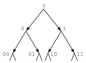
Figure 1. Infinite binary tree $\mathbf{T}$.

The main subject of this section is the group ${\text{\rm Aut}}(\mathbf{T})$ of automorphisms of $\mathbf{T}$, i.e. the group of bijections $\tau:V\to V$ which map edges into edges. Note that the root r is always a fixed point of $\tau$. In other words, $\tau({\text{\bf r}})={\text{\bf r}}$ for all $\tau\in{\text{\rm Aut}}(\mathbf{T})$. More generally, all automorphisms $\tau\in{\text{\rm Aut}}(\mathbf{T})$ preserve the level of vertices: $|\tau(v)|=|v|$, for all $v\in V$. Denote by ${\text{\small{\rm{I}}}}\in{\text{\rm Aut}}(\mathbf{T})$ a trivial (identity) automorphism of $\mathbf{T}$.

An example of a nontrivial automorphism $a\in{\text{\rm Aut}}(\mathbf{T})$ is given in Figure 2. This is the most basic automorphism which will be used throughout the paper, and can be formally defined as follows. Denote by $\mathbf{T}_{\text{\bf 0}}$ and $\mathbf{T}_{\text{\bf 1}}$ the left and right subtrees (branches) of the tree $\mathbf{T}$, with roots at 0 and 1, respectively. Let $a$ be an automorphism which maps $\mathbf{T}_{\text{\bf 0}}$ into $\mathbf{T}_{\text{\bf 1}}$ and preserves the natural order on vertices:

$$\tau:\,({\text{\bf 0}},x_{1},x_{2},\ldots)\longleftrightarrow({\text{\bf 1}},x_{1},x_{2},\ldots).$$

Clearly, automorphism $a$ is an involution: $a^{2}={\text{\small{\rm{I}}}}$.

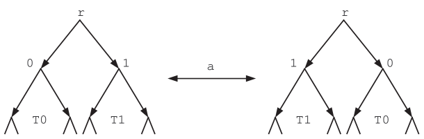
Figure 2. Automorphism $a\in{\text{\rm Aut}}(\mathbf{T})$.

Similarly, one can define an automorphism $a_{v}$ which exchanges two branches $\mathbf{T}_{v{\text{\bf 0}}}$ and $\mathbf{T}_{v{\text{\bf 1}}}$ of a subtree $\mathbf{T}_{v}$ rooted in $v\in V$. These automorphisms will be used in the next section to define finitely generated subgroups of ${\text{\rm Aut}}(\mathbf{T})$.

More generally, denote by ${\text{\rm Aut}}(\mathbf{T}_{v})$ the subgroup of automorphisms in ${\text{\rm Aut}}(\mathbf{T})$ which preserve subtree $T_{v}$ and are trivial on the outside of $T_{v}$. There is a natural graph isomorphism $\iota_{v}:\mathbf{T}\to\mathbf{T}_{v}$ which extends to a group isomorphism $\iota_{v}:{\text{\rm Aut}}(\mathbf{T})\to{\text{\rm Aut}}(\mathbf{T}_{v})$.

By definition, every automorphism $\tau\in{\text{\rm Aut}}(\mathbf{T})$ maps two edges leaving vertex $v$ into two edges leaving vertex $\tau(v)$. Thus we can define a sign $\epsilon_{v}(\tau)\in\{0,1\}$ as follows:

$$\epsilon_{v}(\tau)=\left\{\begin{aligned} &0,\ \ \ \text{if}\ \ \,\tau(v{\text{\bf 0}})=\tau(v){\text{\bf 0}},\ \,\tau(v{\text{\bf 1}})=\tau(v){\text{\bf 1}},\\ &1,\ \ \ \text{if}\ \ \,\tau(v{\text{\bf 0}})=\tau(v){\text{\bf 1}},\ \,\tau(v{\text{\bf 1}})=\tau(v){\text{\bf 0}}.\end{aligned}\right.$$

In other words, $\epsilon_{v}(\tau)$ is equal to $0$ if the automorphism maps the left edge leaving vertex $v$ into the left edge leaving $\tau(v)$, and is equal to $1$ if the automorphism maps the left edge leaving $v$ into the right edge leaving $\tau(v)$.

Observe that the collection of signs $\{\epsilon_{v}(\tau),v\in\mathbf{T}\}$ can take all possible values, and uniquely determines the automorphism $\tau\in{\text{\rm Aut}}(\mathbf{T})$. As a corollary, the group ${\text{\rm Aut}}(\mathbf{T})$ is uncountable and cannot be finitely generated.

To further understand the structure of ${\text{\rm Aut}}(\mathbf{T})$, consider a map

$$\varphi:\ {\text{\rm Aut}}(\mathbf{T})\times{\text{\rm Aut}}(\mathbf{T})\,\to\,{\text{\rm Aut}}(\mathbf{T}),$$

defined as follows. If $\tau_{0},\tau_{1}\in{\text{\rm Aut}}(\mathbf{T})$, let $\tau=\varphi(\tau_{0},\tau_{1})$ be an automorphism defined by $\tau:=\iota_{\text{\bf 0}}(\tau_{0})\cdot\iota_{\text{\bf 1}}(\tau_{1})\in{\text{\rm Aut}}(\mathbf{T})$. Here $\iota_{\text{\bf 0}}(\tau_{0})\in{\text{\rm Aut}}(\mathbf{T}_{\text{\bf 0}})$ and $\iota_{\text{\bf 1}}(\tau_{1})\in{\text{\rm Aut}}(\mathbf{T}_{\text{\bf 1}})$ are the automorphisms of subtrees $\mathbf{T}_{\text{\bf 0}}$ and $\mathbf{T}_{1}$, respectively, defined as above. Pictorially, automorphism $\tau$ is shown in Figure 3.

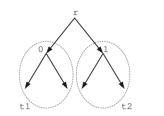
Figure 3. Automorphism $\tau=\varphi(\tau_{0},\tau_{1})\in{\text{\rm Aut}}(\mathbf{T})$.

For any group $G$, the wreath product $G\wr\mathbb{Z}_{2}$ is defined as a semidirect product $(G\times G)\rtimes\mathbb{Z}_{2}$, with $\mathbb{Z}_{2}$ acting by exchanging two copies of $G$.

Proposition 3.1.

${\text{\rm Aut}}(\mathbf{T})\simeq{\text{\rm Aut}}(\mathbf{T})\wr\mathbb{Z}_{2}$.

Proof.

Let us extend the map $\varphi$ to an isomorphism

$$\varphi:\ \bigl{(}{\text{\rm Aut}}(\mathbf{T})\times{\text{\rm Aut}}(\mathbf{T})\bigr{)}\rtimes\mathbb{Z}_{2}\,\longrightarrow\,{\text{\rm Aut}}(\mathbf{T})$$

as follows. When $\sigma={\text{\small{\rm{I}}}}$, let $\varphi(\tau_{0},\tau_{1};\sigma):=\varphi(\tau_{0},\tau_{1})$, as before. When $\sigma\neq{\text{\small{\rm{I}}}}$, let $\varphi(\tau_{0},\tau_{1};\sigma):=\varphi(\tau_{0},\tau_{1})\cdot a$, where $a\in{\text{\rm Aut}}(\mathbf{T})$ is defined as above. Now check that multiplication of automorphisms $\varphi(\cdot)$ coincides with that of the semidirect product, and defines the group isomorphism. We leave this easy verification to the reader. ∎

We denote by $\psi=\varphi^{-1}$ the isomorphism $\psi:{\text{\rm Aut}}(\mathbf{T})\to{\text{\rm Aut}}(\mathbf{T})\wr\mathbb{Z}_{2}$ defined in the proof above. This notation will be used throughout the paper.

Exercise 3.2.

Let ${\text{\rm A}}_{m}\subset{\text{\rm Aut}}(\mathbf{T})$ be a subgroup of all automorphisms $\tau\in{\text{\rm Aut}}(\mathbf{T})$ such that $\epsilon_{v}(\tau)=0$ for all $|v|\geq m$. For example, ${\text{\rm A}}_{1}=\{{\text{\small{\rm{I}}}},a\}$. Use the idea above to show that

$${\text{\rm A}}_{m}\simeq\mathbb{Z}_{2}\,\wr\,\mathbb{Z}_{2}\,\wr\,\cdots\,\wr\,\mathbb{Z}_{2}\ \ \ (m\ \text{times}).$$

Conclude from here that the order of $\,{\text{\rm A}}_{m}$ is $\,|\,{\text{\rm A}}_{m}|\,=\,2^{2^{m}-1}$.

Exercise 3.3.

Consider a (unique) tree automorphism $\tau\in{\text{\rm Aut}}(\mathbf{T})$ with signs given by: $\epsilon_{v}(\tau)=1$ if $v={\text{\bf 1}}^{k}={\text{\bf 1}}\ldots{\text{\bf 1}}$ ($k$ times), for $k\geq 0$, and $\epsilon_{v}(\tau)=0$ otherwise. Check that $\tau$ has infinite order in ${\text{\rm Aut}}(\mathbf{T})$.

Hint: Consider elements $\tau_{m}\in{\text{\rm A}}_{m}$ with signs as in the definition of above, and $k<m$. Show that the order ${\text{\rm ord}}(\tau_{m})\to\infty$ as $m\to\infty$, and deduce the result from here.

4. The first construction

In this section we define a finitely generated group $\mathbb{G}\subset{\text{\rm Aut}}(\mathbf{T})$ which we call the first construction. Historically, this is the first example of a group with intermediate growth [4].

Let us first define group $\mathbb{G}$ implicitly, by specifying the necessary conditions on generators. Let $\mathbb{G}=\langle a,b,c,d\rangle\subset{\text{\rm Aut}}(\mathbf{T})$, where $a$ is the automorphism defined as in Section 3, and automorphisms $b$, $c$, $d$ satisfy the following conditions:

$$(\circ)\ \ \ b=\varphi(a,c),\ \ c=\varphi(a,d),\ \ d=\varphi({\text{\small{\rm{I}}}},b).$$

Observe that the automorphisms $b$, $c$, and $d$ are defined through each other. Since the generator $d$ is acting as identity automorphism on the left subtree $\mathbf{T}_{\text{\bf 0}}$, and as $b$ on the right subtree $\mathbf{T}_{\text{\bf 1}}$, one can recursively compute the action of all three automorphisms $b,c,d\in{\text{\rm Aut}}(\mathbf{T})$.

Here is a direct way to define automorphisms $b,c,d$ :

$$(\ast)\ \ \ \ \begin{aligned} b\,&:=\,(a_{{\text{\bf 0}}}\ \cdot\,a_{{\text{\bf 1}}^{3}{\text{\bf 0}}}\,\cdot\,a_{{\text{\bf 1}}^{6}{\text{\bf 0}}}\cdot\ldots)\,(a_{{\text{\bf 1}}{\text{\bf 0}}}\ \cdot\,a_{{\text{\bf 1}}^{4}{\text{\bf 0}}}\,\cdot\,a_{{\text{\bf 1}}^{7}{\text{\bf 0}}}\cdot\ldots),\\ c\,&:=\,(a_{{\text{\bf 0}}}\,\cdot\,a_{{\text{\bf 1}}^{3}{\text{\bf 0}}}\,\cdot\,a_{{\text{\bf 1}}^{6}{\text{\bf 0}}}\cdot\ldots)\,(a_{{\text{\bf 1}}^{2}{\text{\bf 0}}}\ \cdot\,a_{{\text{\bf 1}}^{5}{\text{\bf 0}}}\,\cdot\,a_{{\text{\bf 1}}^{8}{\text{\bf 0}}}\cdot\ldots),\\ d\,&:=\,(a_{{\text{\bf 1}}{\text{\bf 0}}}\ \cdot\,a_{{\text{\bf 1}}^{4}{\text{\bf 0}}}\,\cdot\,a_{{\text{\bf 1}}^{7}{\text{\bf 0}}}\cdot\ldots)(a_{{\text{\bf 1}}^{2}{\text{\bf 0}}}\,\cdot\,a_{{\text{\bf 1}}^{5}{\text{\bf 0}}}\,\cdot\,a_{{\text{\bf 1}}^{8}{\text{\bf 0}}}\cdot\ldots),\end{aligned}$$

where ${\text{\bf 1}}^{m}$ is short for ${\text{\bf 1}}\ldots{\text{\bf 1}}$ ($m$ times). Note that the automorphisms $a_{{\text{\bf 1}}^{m}{\text{\bf 0}}}$ used in $(\ast)$ commute with each other, and thus elements $b,c,d\in{\text{\rm Aut}}(\mathbf{T})$ are well defined.

Elements $b,c,d\in{\text{\rm Aut}}(\mathbf{T})$ are graphically shown in Figure 4. Here black triangles in vertices of trees represent the subtrees swaps.

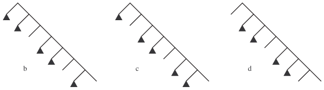
Figure 4. Elements $b,c$ and $d\in{\text{\rm Aut}}(\mathbf{T})$.

Theorem 4.1 (Main Theorem).

Group $\mathbb{G}=\langle a,b,c,d\rangle$ has intermediate growth.

The proof of Theorem 4.1 is quite involved and occupies much of the rest of the paper.

Exercise 4.2.

Check that elements $b,c,d\in{\text{\rm Aut}}(\mathbf{T})$ defined by $(\ast)$ satisfy conditions $(\circ)$.

Exercise 4.3.

Check that elements $b,c$, and $d$ are involutions (have order 2), commute with each other, and satisfy   $b\cdot c\cdot d={\text{\small{\rm{I}}}}$. Conclude from here that $\langle b,c,d\rangle\simeq\mathbb{Z}_{2}^{2}$ and that the group $\mathbb{G}=\langle a,b,c,d\rangle$ is $3$-generated.

Exercise 4.4.

Check the following relations in $\mathbb{G}:$   $(ad)^{4}=(ac)^{8}=(ab)^{16}={\text{\small{\rm{I}}}}$. Deduce from here that 2-generator subgroups $\langle a,b\rangle,\langle a,c\rangle,\langle a,d\rangle\subset\mathbb{G}$ are finite.

While these exercises have straightforward ‘verification style’ proofs, they will prove useful in the future. Thus we suggest the reader studies them before proceeding to read (hopefully) the rest of the paper.

5. Group $\mathbb{G}$ is infinite

We have yet to establish that $\mathbb{G}$ is infinite. Although one can prove this directly, the proof below introduces definitions and notation which will be helpful in the future.

Let ${\text{\rm St}}_{\mathbb{G}}(n)$ denote a subgroup of $\mathbb{G}$ stabilizing all vertices with level $n$. In other words, ${\text{\rm St}}_{\mathbb{G}}(n)$ consists of all automorphisms $\tau\in\mathbb{G}$ such that $\tau(v)=v$ for all vertices $v\in\mathbf{T}$ with $|v|=n$:

$${\text{\rm St}}_{\mathbb{G}}(n)\,=\,\bigcap_{|v|=n}{\text{\rm St}}_{\mathbb{G}}(v).$$

The subgroup $\mathbb{H}:={\text{\rm St}}_{\mathbb{G}}(1)$ is called the fundamental subgroup of $\mathbb{G}$.

Lemma 5.1.

Let $\mathbb{H}\subset\mathbb{G}$ be the fundamental subgroup defined above. Then:

$$\mathbb{H}=\langle b,c,d,b^{a},c^{a},d^{a}\rangle,\quad\mathbb{H}\lhd\mathbb{G},\ \ \ \text{and}\ \ \ [\mathbb{G}:\mathbb{H}]=2.$$

Proof.

From Exercise 4.3 we conclude that every reduced decomposition $w$ is a product $w=(a)\ast a\ast a\ast\ldots\ast a\ast(a)$, where each $\ast$ is either $b$, $c$, or $d$, while the first and last $a$ may or may not appear. Denote by $|w|$ the length of the word $w$, and by $|w|_{a}$ the number of occurrences of $a$ in $w$. Note that $w\in\mathbb{H}$ if and only if $|w|_{a}$ is even. This immediately implies the third part of the lemma. Since every subgroup of index 2 is normal this also implies the second part.

For the first part, suppose $|w|_{a}$ is even. Join subsequent occurrences of $a$ to obtain $w$ as a product of $\ast$ and $(a\ast a)$. Since $a^{2}={\text{\small{\rm{I}}}}$, we have $(a\ast a)=\ast^{a}$, which implies the result. ∎

This following exercise generalizes the second part of Lemma 5.1 and will be used in Section 9 to prove the upper bound on the growth function of $\mathbb{G}$.

Exercise 5.2.

Check that the stabilizer subgroup $\mathbb{H}_{n}:={\text{\rm St}}_{\mathbb{G}}(n)$ has finite index in $\mathbb{G}:$ $[\mathbb{G}:\mathbb{H}_{n}]\leq|\,{\text{\rm A}}_{n}|=2^{2^{n}-1}$ (see Exercise 3.2).

Let $\psi=\varphi^{-1}:{\text{\rm Aut}}(\mathbf{T})\to\bigl{(}{\text{\rm Aut}}(\mathbf{T})\times{\text{\rm Aut}}(\mathbf{T})\bigr{)}\rtimes\mathbb{Z}_{2}$ be the isomorphism defined in Section 3. By definition, $\mathbb{H}\subset\mathbb{G}\subset{\text{\rm Aut}}(\mathbf{T})$.

Lemma 5.3.

The image $\psi(\mathbb{H})$ is a subgroup of $\mathbb{G}\times\mathbb{G}$, such that projection of $\psi(\mathbb{H})$ onto each component is surjective.

Proof.

By definition, $\mathbb{H}$ stabilizes 0 and 1, so $\psi(\mathbb{H})\subset{\text{\rm Aut}}(\mathbf{T})\times{\text{\rm Aut}}(\mathbf{T})$. From Exercise 4.2 we have

$$\psi:\ \ \left\{\begin{aligned} &\ b\to(a,c)\,,\ \qquad b^{a}\to(c,a)\,,\\ &\ c\to(a,d)\,,\ \qquad c^{a}\to(d,a)\,,\\ &\ d\to({\text{\small{\rm{I}}}},b)\,,\ \qquad d^{a}\to(b,{\text{\small{\rm{I}}}})\,.\end{aligned}\right.$$

Now Lemma 5.1 implies that $\psi(\mathbb{H})\subset\mathbb{G}\times\mathbb{G}$. On the other hand, the projection of $\psi(\mathbb{H})$ onto each component contains all four generators $a,b,c,d\in\mathbb{G}$, and is therefore surjective. ∎

Corollary 5.4.

Group $\mathbb{G}$ is infinite.

Proof.

From Lemma 5.1 and Lemma 5.3 above, we have $\mathbb{H}$ is a proper subgroup of $\mathbb{G}$ which is mapped surjectively onto $\mathbb{G}$. If $|\mathbb{G}|<\infty$, then $|\mathbb{G}|>|\mathbb{H}|\geq|\mathbb{G}|$, a contradiction. ∎

Here is a different application of Lemma 5.3. Let $G\subset{\text{\rm Aut}}(\mathbf{T})$ be a subgroup of the group automorphisms of the binary tree $\mathbf{T}$. Denote by $G_{v}={\text{\rm St}}_{G}(v)|_{\mathbf{T}_{v}}\subset{\text{\rm Aut}}(\mathbf{T}_{v})$ the subgroup of $G$ of elements which fix vertex $v\in\mathbf{T}$ with the action restricted only to the subtree $\mathbf{T}_{v}$. We say that $G$ has (strong) self-similarity property if $G_{v}\simeq G$ for all $v\in\mathbf{T}$.

Corollary 5.5.

Group $\mathbb{G}$ has self-similarity property.

Proof.

Use the induction on the level $|v|$. By definition, $\mathbb{G}_{\text{\bf r}}=\mathbb{G}$, and by Lemma 5.3 we have $\mathbb{G}_{\text{\bf 0}},\mathbb{G}_{1}\simeq\mathbb{G}$. For general $v\in\mathbf{T}$ we similarly have $\mathbb{G}_{v{\text{\bf 0}}},\mathbb{G}_{v{\text{\bf 1}}}\simeq\mathbb{G}_{v}$. This implies the result. ∎

Exercise 5.6.

Consider the following rewriting rules:

$$\eta:\,a\to aba,\ \ b\to d,\ \ c\to b,\ \ d\to c$$

Define a sequence of elements in $\mathbb{G}$: $x_{1}=a$ and $x_{i+1}:=\eta(x_{i})$ for all $i\geq 1$. Prove directly that all these elements are distinct. Conclude from here that $\mathbb{G}$ is infinite.

6. Superpolynomial growth of $\mathbb{G}$

In this section we prove the first half of Theorem 4.1, by showing that the growth function $\gamma$ of group $\mathbb{G}$ satisfies conditions of the Lower Bound Lemma.

Two groups $G_{1}$ and $G_{2}$ are called commeasurable, denotes $G_{1}\approx G_{2}$, if they contain isomorphic subgroups of finite index:

$$H_{1}\subset G_{1},\,H_{2}\subset G_{2},\,\ H_{1}\simeq H_{2},\ \ \text{and}\ \ [G_{1}:H_{1}],\,[G_{2}:H_{2}]<\infty.$$

For example, group $\mathbb{Z}$ is commeasurable with the infinite dihedral group $\textsc{D}_{\infty}\simeq\mathbb{Z}\rtimes\mathbb{Z}_{2}$. Of course, all finite groups are commeasurable to each other. Another example is $\mathbb{H}\approx\mathbb{G}$, since $\mathbb{H}$ is a subgroup of finite index in $\mathbb{G}$. Note also that commeasurability is an equivalence relation.

Proposition 6.1.

Groups $\mathbb{G}$ and $\mathbb{G}\times\mathbb{G}$ are commeasurable: $\mathbb{G}\approx\mathbb{G}\times\mathbb{G}$.

Proposition 6.1 describes an important phenomenon which can be formalized as follows. The group $G$ is called multilateral if $G$ is infinite and $G\approx G^{m}$ for some $m\geq 2$. As we show below, all such groups have superpolynomial growth.

To prove the proposition, consider the subgroups $\mathbb{H}\subset\mathbb{G}$ and $\widetilde{\mathbb{H}}:=\psi(\mathbb{H})\subset\mathbb{G}\times\mathbb{G}$. By Lemma 5.1 we have $[\mathbb{G}:\mathbb{H}]<\infty$. Since $\psi$ is a group isomorphism, we also have $\widetilde{\mathbb{H}}\simeq\mathbb{H}$. If we show that $[\mathbb{G}\times\mathbb{G}:\widetilde{\mathbb{H}}]<\infty$, then $\mathbb{G}\approx\mathbb{G}\times\mathbb{G}$, as claimed in Proposition 6.1.

Denote by $\mathbb{B}=\langle b\rangle^{G}$ the normal closure of $b\in\mathbb{G}$, defined as $\mathbb{B}:=\langle g^{-1}bg\mid g\in\mathbb{G}\rangle$.

Lemma 6.2.

Subgroup $\mathbb{B}$ has a finite index in $\mathbb{G}$. More precisely, $[\mathbb{G}:\mathbb{B}]\leq 8$.

Proof.

By Exercise 4.4, we have $a^{2}=d^{2}=(ad)^{4}={\text{\small{\rm{I}}}}$. It is easy to see now that the 2-generated subgroup $\langle a,d\rangle\subset\mathbb{G}$ is a dihedral group $D_{4}$ of order 8. By Exercise 4.3, we have $\mathbb{G}=\langle a,b,d\rangle$. Therefore, $\mathbb{G}/\mathbb{B}$ is a quotient of $\langle a,d\rangle$, and $[\mathbb{G}:\mathbb{B}]\leq|D_{4}|=8$. ∎

Lemma 6.3.

Subgroup $\widetilde{\mathbb{H}}=\psi(\mathbb{H})$ contains $\mathbb{B}\times\mathbb{B}\subset\mathbb{G}\times\mathbb{G}$.

Proof.

By Lemma 5.1, we know that $\widetilde{\mathbb{H}}\supset\langle\psi(d),\psi(d^{a})\rangle=\langle(1,b),(b,1)\rangle$. Let $x\in\mathbb{H}$ and $\psi(x)=(x_{0},x_{1})$. We have:

$$\psi(d^{x}) =\,\psi(x^{-1}dx)\,=\,\psi(x^{-1})\,\psi(d)\,\psi(x)\,=\,(x_{0}^{-1},x_{1}^{-1})\,({\text{\small{\rm{I}}}},b)\,(x_{0},x_{1})$$

$$=\,({\text{\small{\rm{I}}}},x_{1}^{-1}bx_{1})\,=\,({\text{\small{\rm{I}}}},b^{x_{1}}).$$

By Lemma 5.3, here we can take any element $x_{1}\in\mathbb{G}$. Therefore, the image $\psi(\mathbb{H})$ contains all elements of the form $({\text{\small{\rm{I}}}},b^{g})$, $g\in\mathbb{G}$. By definition, these elements generate a subgroup $1\times\mathbb{B}$. In other words, $\widetilde{\mathbb{H}}=\psi(\mathbb{H})\supset 1\times\mathbb{B}$. Similarly, using the element $d^{a}$ in place of $d$, we obtain $\widetilde{\mathbb{H}}\supset\mathbb{B}\times 1$. Therefore, $\widetilde{\mathbb{H}}\supset\mathbb{B}\times\mathbb{B}$, as desired. ∎

Now Proposition 6.1 follows immediately once we note that $\mathbb{B}\times\mathbb{B}\subset\widetilde{\mathbb{H}}\subset\mathbb{G}\times\mathbb{G}$, and by Lemma 6.2 the index

$$[\mathbb{G}\times\mathbb{G}:\widetilde{\mathbb{H}}]\,\leq\,[\mathbb{G}\times\mathbb{G}:\mathbb{B}\times\mathbb{B}]\,=\,[\mathbb{G}:\mathbb{B}]^{2}\,\leq\,8^{2}\,=\,64.$$

Since $\mathbb{G}$ is infinite (Corollary 5.4) this implies that group $\mathbb{G}$ is multilateral.  $\square$

Lemma 6.4.

Every multilateral group $G$ has superpolynomial growth. Moreover, the growth function $\gamma_{G}(n)\succcurlyeq\exp(n^{\alpha})$ for some $\alpha>0$.

Proof.

By definition, $G$ is infinite, and $G\approx G^{m}$ for some $m>1$. In other words, there exist $H\subset G$, $\widetilde{H}\subset G^{m}$ such that $H\simeq\widetilde{H}$ and $[G:H],[G^{m}:\widetilde{H}]<\infty$. From Exercise 1.5 we obtain $\gamma_{G}\sim\gamma_{H}\sim\gamma_{\widetilde{H}}\sim\gamma_{G^{m}}$. Thus $\gamma_{G}\succcurlyeq\gamma_{G^{m}}$, and the Lower Bound (Lemma 2.1) implies the result. ∎

Now Proposition 6.1 and Lemma 6.4 immediately imply the first part of Theorem 4.1:

Corollary 6.5.

Group $\mathbb{G}$ has superpolynomial growth. Moreover, the growth function $\gamma_{\mathbb{G}}(n)\succcurlyeq\exp(n^{\alpha})$ for some $\alpha>0$.

7. Length of elements and rewriting rules

To prove the second half of Theorem 4.1 we derive sharp upper bounds on the growth function $\gamma=\gamma_{\mathbb{G}}^{S}$ of the group $\mathbb{G}$ with the generating set $S=\{a,b,c,d\}$. In this section we obtain some recursive bounds on the length $\ell(g)=\ell_{\mathbb{G}}^{S}(g)$ of elements $g\in\mathbb{G}$ in terms of $S$. Note that although $\mathbb{G}$ is 3-generated, having the fourth generator is convenient for technical reasons.

We begin with a simple classification of reduced decompositions of elements of $\mathbb{G}$ following the approach in the proof of Lemma 5.1. We define four types of reduced decompositions:

$({\text{\rm i}})$       if  $g=a\ast a\ast a\cdots\ast a\ast a$,

$({\text{\rm i}}{\text{\rm i}})$      if  $g=a\ast a\ast a\cdots\ast a\,\ast$,

$({\text{\rm i}}{\text{\rm i}}{\text{\rm i}})$   if  $g=\ast\,a\ast a\ast\cdots a\ast a$,

$({\text{\rm i}}{\text{\rm v}})$   if  $g=\ast\,a\ast a\ast\cdots a\ast a\,\hskip 0.42677pt\ast$.

Of course, element $g$ can have many different reduced decompositions. On the other hand, the type of a decomposition is almost completely determined by $g$.

Lemma 7.1.

Every group element $g\in\mathbb{G}$ has all of its reduced decompositions of the same type $({\text{\rm i}})$, or of type $({\text{\rm i}}{\text{\rm v}})$, or of type $({\text{\rm i}}{\text{\rm i}})$ and $({\text{\rm i}}{\text{\rm i}}{\text{\rm i}})$.

Proof.

Recall that the number of $a$’s in a reduced decomposition of $g\in\mathbb{G}$ is even if $g\in\mathbb{H}$, and is odd otherwise. Thus $g$ cannot have decompositions of type $({\text{\rm i}})$ and $({\text{\rm i}}{\text{\rm v}})$ at the same time. Noting that decompositions of type $({\text{\rm i}})$ and $({\text{\rm i}}{\text{\rm v}})$ have odd length while those of type $({\text{\rm i}}{\text{\rm i}})$ and $({\text{\rm i}}{\text{\rm i}}{\text{\rm i}})$ have even length implies the result. ∎

It is easy to see that one cannot strengthen Lemma 7.1 since some elements can have decompositions of both type $({\text{\rm i}}{\text{\rm i}})$ and $({\text{\rm i}}{\text{\rm i}}{\text{\rm i}})$. For example, $adad=dada$ by Exercise 4.3, and both are reduced decompositions. From this point on we refer to elements $g\in\mathbb{G}$ as of type $({\text{\rm i}})$, $({\text{\rm i}}{\text{\rm i}}/{\text{\rm i}}{\text{\rm i}}{\text{\rm i}})$, or $({\text{\rm i}}{\text{\rm v}})$ depending on the type of their reduced decompositions.

In the next lemma we use the isomorphism $\psi=\varphi^{-1}:{\text{\rm Aut}}(\mathbf{T})\to{\text{\rm Aut}}(\mathbf{T})\wr S_{2}$, where $S_{2}=\{{\text{\small{\rm{I}}}},a\}\simeq\mathbb{Z}_{2}$.

Lemma 7.2.

Let $\ell(g)$ be the length of $g\in\mathbb{G}$ in generators $S=\{a,b,c,d\}$. Suppose $\psi(g)=(g_{0},g_{1};\sigma)$, where $g_{0},g_{1}\in\mathbb{G}$ and $\sigma\in S_{2}$. Then:

$\ell(g_{0}),\ell(g_{1})\leq\frac{1}{2}(\ell(g)-1)$ if $g$ has type $({\text{\rm i}})$,

$\ell(g_{0}),\ell(g_{1})\leq\frac{1}{2}\,\ell(g)$ if $g$ has type $({\text{\rm i}}{\text{\rm i}}/{\text{\rm i}}{\text{\rm i}}{\text{\rm i}})$,

$\ell(g_{0}),\ell(g_{1})\leq\frac{1}{2}(\ell(g)+1)$ if $g$ has type $({\text{\rm i}}{\text{\rm v}})$.

Proof.

Fix an element $g\in\mathbb{G}$, and let $g_{0},g_{1},\sigma$ be as in the lemma. We have $\sigma={\text{\small{\rm{I}}}}$ if $g\in\mathbb{H}$, and $\sigma=a$ otherwise (see the proof of Lemma 5.1). For every reduced decomposition $w=(a)\ast a\ast a\cdots\ast a\ast(a)$ of $g$ we shall construct decompositions of elements $g_{0},g_{1}$ with lengths as in the lemma. As before, we use $\ast$ to denote either of the generators $b,c,d$. Also, for every $\ast$ in a reduced decomposition denote by $\pi(\ast)$ the number of $a$’s preceding $\ast$.

Consider the following rewriting rules:

$$\Phi_{0}:\ \qquad\left\{\begin{aligned} &a\to{\text{\small{\rm{I}}}},\\ &b\to a,\ \ c\to a,\ \ d\to{\text{\small{\rm{I}}}}\ \ \ \text{if}\ \ \,\pi(\ast)\ \ \,\text{is odd,}\\ &b\to c,\ \ c\to d,\ \ \hskip 0.42677pt\hskip 0.42677ptd\to b\ \ \ \text{if}\ \ \,\pi(\ast)\ \ \,\text{is even,}\end{aligned}\right.$$

and

$$\Phi_{1}:\ \qquad\left\{\begin{aligned} &a\to{\text{\small{\rm{I}}}},\\ &b\to a,\ \ c\to a,\ \ d\to{\text{\small{\rm{I}}}}\ \ \ \text{if}\ \ \,\pi(\ast)\ \ \,\text{is even,}\\ &b\to c,\ \ c\to d,\ \ \hskip 0.42677pt\hskip 0.42677pt\hskip 0.42677ptd\to b\ \ \ \text{if}\ \ \,\pi(\ast)\ \ \,\text{is odd.}\end{aligned}\right.$$

These rules act on words $w$ in generators $S$, and substitute each occurrence of a letter with the corresponding letter or I.

Let $\Phi_{0}(w)$, $\Phi_{1}(w)$ be the words obtained from the word $w=(a)\ast a\cdots a\ast(a)$ by the rewriting rules as above, and let $g^{\prime}_{0},g^{\prime}_{1}\in\mathbb{G}$ be group elements defined by these products. Check by induction on the length $\ell(g)$ that $\psi(g)=(g^{\prime}_{0},g^{\prime}_{1};\sigma)$. Indeed, note that the rules give the first and second components in the formula for $\psi$ in the proof of Lemma 5.3. Now, as in the proof of Lemma 5.1 subdivide the product $w$ into elements $(a)$ and $(\ast\,\hskip 0.42677pta\hskip 0.42677pt\ast)$, and obtain the induction step. From here we have $g_{0}=g^{\prime}_{0}$, $g_{1}=g^{\prime}_{1}$, and by construction of rewriting rules the lengths of $g_{0},g_{1}$ are as in the lemma. ∎

As we show below, the rewriting rules are very useful in the study of group $\mathbb{G}$, but also in a more general setting.

Corollary 7.3.

In conditions of Lemma 7.2 we have: $\ell(g_{0})+\ell(g_{1})\leq\ell(g)+1$.

The above corollary is not tight and can be improved in certain cases. The following exercise give bounds in the other direction, limiting potential extensions of Corollary 7.3.

Exercise 7.4.

In conditions of Lemma 7.2 we have: $\ell(g)\leq 2\ell(g_{0})+2\ell(g_{1})+50$.

This result can be used to show that $\gamma_{\mathbb{G}}\succcurlyeq\exp(\sqrt{n})$. The proof is more involved that of other exercises; it will not be used in this paper.

Exercise 7.5.

Prove that every element $g\in\mathbb{G}$ has order $2^{k}$, for some integer $k$.  Hint: use induction to reduce the problem to elements $g_{0}$, $g_{1}$ (cf. Lemma 7.2).

8. The word problem

The classical word problem can be formulated as follows: given a word $w=s_{i_{1}}\cdots s_{i_{n}}$ in generators $s_{j}\in S$, decide whether this product is equal to I in $G=\langle S\rangle$. To set up the problem carefully one would have to describe presentation of the group and allowed operations [8]. We skip these technicalities in hope that the reader has an intuitive understanding of the problem.

Now, from the algorithmic point of view the problem is undecidable, i.e. there is no Turing machine which can resolve it in finite time for every group. On the other hand, for certain groups the problem can be solved very efficiently, in time polynomial in the length $n$ of the product. For example, in the free group $F_{k}=\langle x_{1}^{\pm 1},\ldots,x_{k}^{\pm 1}\rangle$ the problem can be solved in linear time: take a product $w$ and repeatedly cancel every occurrence of $x_{i}x_{i}^{-1}$ and $x_{i}^{-1}x_{i}$, $1\leq i\leq k$; the product $w={\text{\small{\rm{I}}}}$ if and only if the resulting word is empty. Since every letter is cancelled at most once and new letters are not created, the algorithm takes $O(n)$ cancellations.

Exercise 8.1.

Note that the above algorithm as defined one might need to search for the next cancellation, increasing the complexity of the algorithm to as much as $O(n^{2})$. Modify the algorithm by using a single stack to prove that word problem in $F_{k}$ can in fact be solved in linear time.

The class of groups where the word problem can be solved in linear number of cancellations is called word hyperbolic. This class has a simple description and many group theoretic applications [7]. The following result shows that word problem can be resolved in $\mathbb{G}$ in nearly linear time.

Theorem 8.2.

The word problem in $\mathbb{G}$ can be solved in $O(n\log n)$ time.

Proof.

Consider the following algorithm. First, cancel products of $b,c,d$ to write the word as $w=(a)\ast a\ast\cdots\ast a\ast(a)$. If the number $\pi(w)$ of $a$’s is odd, then the product $w\neq_{\mathbb{G}}{\text{\small{\rm{I}}}}$. If the $\pi(w)$ is even, use the rewriting rules (proof of Lemma 7.2) to obtain words $w_{0}=\Phi_{0}(w)$ and $w_{1}=\Phi_{1}(w)$ (which may no longer by reducible). Recall that the product $w=_{\mathbb{G}}{\text{\small{\rm{I}}}}$ if and only if $w_{0},w_{1}=_{\mathbb{G}}{\text{\small{\rm{I}}}}$. Now repeat the procedure for the words $w_{0},w_{1}$ to obtain words $w_{00},w_{01},w_{10},w_{11}$, etc. Check that $w=_{\mathbb{G}}{\text{\small{\rm{I}}}}$ if and only if eventually all the obtained words are trivial.

Observe that the length of each word $w_{i}$ is at most $(n+1)/2$. Iterating this bound, we conclude that the number of ‘rounds’ in the algorithm of constructing smaller and smaller words is $O(\log n)$. Therefore, each letter is replaced at most $O(\log n)$ times and thus the algorithm finishes in $O(n\log n)$ time. ∎

Remark 8.3.

For every reduced decomposition as above one can construct a binary tree of nontrivial words $w_{i_{1}i_{2}\dots i_{r}}$. The distribution of height and shape (profile) of these trees is closely connected to the growth function $\gamma_{\mathbb{G}}$. Exploring this connection is of great interest, but lies outside the scope of this paper.

9. Subexponential growth of $\mathbb{G}$

In this section we prove the second half of Theorem 4.1 by establishing the upper bound on the growth function $\gamma$ of group $\mathbb{G}$ with generators $S=\{a,b,c,d\}$. The proof relies on the technical Cancellation Lemma which will be stated here and proved in the next section.

Let $\mathbb{H}_{3}:={\text{\rm St}}_{\mathbb{G}}(3)$ be the stabilizer of vertices on the third level, and recall that the index $[\mathbb{G}:\mathbb{H}_{3}]\leq 2^{7}=128$ (Exercise 5.2). There is a natural embedding

$$\psi_{3}\,:\,\mathbb{H}_{3}\,\longrightarrow\,\mathbb{G}_{{\text{\bf 0}}{\text{\bf 0}}{\text{\bf 0}}}\times\mathbb{G}_{{\text{\bf 0}}{\text{\bf 0}}{\text{\bf 1}}}\times\ldots\times\mathbb{G}_{{\text{\bf 1}}{\text{\bf 1}}{\text{\bf 1}}}$$

(see Section 5). By self-similarity, each of the eight groups in the product is isomorphic: $\mathbb{G}_{\mathbf{ijk}}\simeq\mathbb{G}$, where $\mathbf{i},\mathbf{j},\mathbf{k}\in\{{\text{\bf 0}},{\text{\bf 1}}\}$. These isomorphisms are obtained by restrictions of natural maps: $\iota_{v}^{-1}:{\text{\rm Aut}}(\mathbf{T}_{v})\to{\text{\rm Aut}}(\mathbf{T})$, where $v\in\mathbf{T}$. Now combine $\psi_{3}$ with the map $(\iota_{{\text{\bf 0}}{\text{\bf 0}}{\text{\bf 0}}}^{-1},\iota_{{\text{\bf 0}}{\text{\bf 0}}{\text{\bf 1}}}^{-1},\ldots,\iota_{{\text{\bf 1}}{\text{\bf 1}}{\text{\bf 1}}}^{-1})$ we obtain a group homomorphism $\chi:\mathbb{H}_{3}\to\mathbb{G}^{8}$ written as $\chi(h)=(g_{000},g_{001},\ldots,g_{111})$, where $h\in\mathbb{H}_{3}$ and $g_{ijk}\in\mathbb{G}$.

It follows easily from Corollary 7.3 that $\ell(g_{000})+\ell(g_{001})+\ldots+\ell(g_{111})\leq\ell(h)+7$. The following result is an improvement over this bound:

Lemma 9.1 (Cancellation Lemma).

Let $h\in\mathbb{H}_{3}$. In the notation above we have:

$$\ell(g_{000})+\ell(g_{001})+\ldots+\ell(g_{111})\,\leq\,\frac{5}{6}\,\ell(h)+8.$$

We postpone the proof of Cancellation Lemma till next section. Now we are ready to finish the proof of the Main Theorem.

Proposition 9.2.

Group $\mathbb{G}$ has subexponential growth. Moreover, $\gamma_{\mathbb{G}}(n)\preccurlyeq\exp(n^{\nu})$ for some $\nu<1$.

Proof.

All elements $g\in\mathbb{G}$ can be written as $g=u\cdot h$ where $h\in\mathbb{H}_{3}$ and $u$ is a coset representative of $\mathbb{G}/\mathbb{H}_{3}$. Since $[\mathbb{G}:\mathbb{H}_{3}]\leq 128$, there are at most 128 such elements $u$. Note that we can choose elements $u$ which have length at most 127 in $S=\{a,b,c,d\}$, since all prefixes of a reduced decomposition can be made to lie in distinct cosets. The decomposition $h=u^{-1}g$ then gives $\ell(h)\leq\ell(g)+127$.

Now write $g=u\hskip 0.42677pth=u\hskip 0.42677ptg_{000}\hskip 0.42677ptg_{001}\cdots g_{111}$. The Cancellation Lemma gives:

$$\sum_{ijk}\ell(g_{ijk})\,\leq\,\,\frac{5}{6}\,\ell(h)+8\,\leq\,\frac{5}{6}\,\bigl{(}\ell(g)+127\bigr{)}+8\,<\,\frac{5}{6}\,\ell(g)+114.$$

Putting all this together we conclude:

$$\gamma(n)\,\leq\,128\sum_{(n_{1},\ldots,n_{8})}\,\gamma(n_{1})\cdots\gamma(n_{8}),$$

where the summation is over all integer $8$-tuples with $n_{1}+\ldots+n_{8}\leq\frac{5}{6}n+114$. Set $m=n+137$ so that $\frac{5}{6}\hskip 0.42677ptn+114<\frac{5}{6}\hskip 0.42677ptm$. Now note that

$$\gamma(m)\,=\,\gamma(n+137)\,\leq\,\gamma(n)\cdot|S|^{137}\,=\,4^{137}\,\gamma(n).$$

Therefore, we have:

$$\gamma(m)\,\leq\,4^{137}\,\gamma(n)\,\leq\,4^{137}\cdot 128\cdot\gamma^{\star\,8}\left(\frac{5}{6}\,n+114\right)\,\leq\,2^{281}\,\gamma^{\star\,8}\left(\frac{5}{6}\,m\right).$$

From here and the Upper Bound (Lemma 2.2) we obtain the result. ∎

Recall that subexponential growth of $\mathbb{G}$ is shown in Corollary 6.5. This completes the proof of Theorem 4.1.  $\square$

10. Proof of the Cancellation Lemma

Fix a reduced decomposition $(a)\ast a\ast a\cdots\ast(a)$ of $h\in\mathbb{H}_{3}$, and denote this decomposition by $w$. Apply rewriting rules $\Phi_{0}$ and $\Phi_{1}$ to $w$ obtain words $w_{0}$ and $w_{1}$. At this moment remove all identities I. Then apply these rules again to obtain $w_{00},w_{01},w_{10}$ and $w_{11}$, and remove the identities I. Finally, repeat this once again to obtain words $w_{000},w_{001},\ldots,w_{111}$. Following the proof of Theorem 8.2, all these words give decompositions of elements $g_{0},g_{1}$, then $g_{00},\ldots,g_{11}$, and $g_{ijk}\in\mathbb{G}_{\textbf{ijk}}$, respectively. Note that these decompositions are not necessarily reduced, so for the record:

$$(\maltese)\ \ \ \ell(g_{i})\leq|w_{i}|,\ \ \ell(g_{ij})\leq|w_{ij}|,\ \ \ell(g_{ijk})\leq|w_{ijk}|,\ \ \ \text{for all}\ \ i,j,k\in\{0,1\},$$

where $|u|$ denotes the length of the word $u$. Also, by Corollary 7.3 we have:

$$(\diamondsuit)\quad\begin{aligned} \ell(g_{0})+\ell(g_{1})&\leq\ell(h)+1,\\ \ell(g_{00})+\ldots+\ell(g_{11})&\leq\ell(g_{0})+\ell(g_{1})+2,\\ \ell(g_{000})+\ell(g_{001})+\ldots+\ell(g_{111})&\leq\ell(g_{00})+\ldots+\ell(g_{11})+4.\end{aligned}\quad$$

To simplify the notation, consider the following concatenations of these words:

$$w^{\prime}=w_{0}\cdot w_{1},\ \ w^{\prime\prime}=w_{00}\cdots w_{11},\ \ \,\text{and}\ \ w^{\prime\prime\prime}=w_{000}\cdot w_{001}\cdots w_{111}.$$

By construction of the rewriting rules, since the only possible cancellation happens when $d\to{\text{\small{\rm{I}}}}$ we have: $|w^{\prime}|\leq|w|+1-|w|_{d}$, where $|w|_{d}$ is the number of letters $d$ in $w$. Indeed, simply note that each letter $d$ in $w$ is cancelled by either $\Phi_{0}$ or $\Phi_{1}$. Unfortunately we cannot iterate this inequality as the words $w_{i}$ are not reduced. Note on the other hand, that each letter $c$ in $w$ produces one letter $d$ in $w^{\prime}$ and each of the latter is cancelled again by either $\Phi_{0}$ or $\Phi_{1}$. Finally, each letter $b$ in $w$ produces one letter $c$ in $w^{\prime}$, which in turn produces letter $d$ in $w^{\prime\prime}$, and each of the latter is cancelled again by either $\Phi_{0}$ or $\Phi_{1}$. Taking into account the types of decompositions we obtain:

$$(\heartsuit)\ \qquad\begin{aligned} |w^{\prime}|\,&\leq\,|w|+1-|w|_{d}\,,\\ |w^{\prime\prime}|\,&\leq\,|w|+3-|w|_{c}\,,\\ |w^{\prime\prime\prime}|\,&\leq\,|w|+7-|w|_{b}\,.\end{aligned}\quad$$

Since $|w|_{b}+|w|_{c}+|w|_{d}\geq(|w|-1)/2$, at least one of the numbers $|w|_{\ast}>|w|/6-1$. Combining this with $(\heartsuit)$, $(\diamondsuit)$, and (✠) we conclude:

$$\ell(g_{000})+\ell(g_{001})+\ldots+\ell(g_{111})\,\leq\,\max\bigl{\{}|w^{\prime}|+2+4,|w^{\prime\prime}|+4,|w^{\prime\prime\prime}|\bigr{\}}\,$$

$$\ \ \ \leq\,|w|+7-\max_{\ast\in\{b,c,d\}}|w|_{\ast}\,\leq\,|w|+7-(|w|/6-1)\,=\,\frac{5}{6}\,\ell(h)+8,$$

as desired.  $\square$

11. Further developments, conjectures and open problems

Much about groups of intermediate growth remains open. Below we include only the most interesting results and conjectures which are closely connected to the material presented in this paper. Everywhere below we refer to surveys [1, 2, 6] and books [8, 11] for details and further references.

Let us start by saying that the Upper Bound and Lower Bound lemmas can be used to obtain effective bounds on the growth function of $\mathbb{G}$. Although considerably sharper bounds are known, the exact asymptotic behavior of $\gamma_{\mathbb{G}}$ remain an open problem. Unfortunately, we do not even know whether it makes sense to say that $\gamma_{\mathbb{G}}$ has growth $\exp(n^{\alpha})$ for some fixed $\alpha>0$:

Conjecture 11.1.

Let $\gamma=\gamma_{\mathbb{G}}$ be the growth function of group $\mathbb{G}$. Prove that there exists a limit $\,\alpha=\lim_{n\to\infty}\log_{n}\log\hskip 0.42677pt\gamma(n)$.

In fact, the limit as in the conjecture is not known to exist and satisfy $0<\alpha<1$ for any finitely generated group. Alternatively, the extend to which results for $\mathbb{G}$ generalize to other groups of intermediate growth remains unclear as well. Although there are now constructions of groups with subexponential growth function $\gamma(n)\sim e^{n\hskip 0.42677pt(1-o(1))}$, there are no known examples of groups with superpolynomial growth function $\gamma(n)\sim\exp(n^{o(1)})$. The following result has been established for a large classes of groups, but not in general:

Conjecture 11.2.

Let $G$ be a group of intermediate growth, and let $\gamma_{G}(n)$ be its growth function. Then $\gamma_{S}(n)\succcurlyeq\exp(n^{\alpha})$ for some $\alpha>0$.

Moving away from the bounds on the growth, let us mention that group $\mathbb{G}$ is not finitely presented. Existence of finitely presented groups of intermediate growth is a major open problem in the field, and the answer is believed to be negative:

Conjecture 11.3.

There are no finitely presented groups of intermediate growth.

Our final conjecture may seem technical and unmotivated as stated. If true it resolves positively the “$p_{c}<1$” conjecture of Benjamini and Schramm on percolation on Cayley graphs.

Conjecture 11.4.

Every group $G$ of intermediate growth contains two infinite subgroups $H_{1}$ and $H_{2}$ which commute with each other: $[h_{1},h_{2}]={\text{\small{\rm{I}}}}$ for all $h_{1}\in H_{1}$ and $h_{2}\in H_{2}$.

We refer to [9] for an overview of this conjecture and its relation to groups of intermediate growth.

Acknowledgements.  We would like to thank Tatiana Nagnibeda and Roman Muchnik the interest in the subject and engaging discussions. Both authors were partially supported by the NSF.

12. Appendix

Proof of the Lower Bound Lemma.  To simplify the notation, let us extend definition of $f$ to the whole line $f:\mathbb{R}_{+}\to\mathbb{R}_{+}$ by setting $f(x):=f(\lfloor x\rfloor)$. Let $\pi(n)=\ln f(n)$. Clearly, $\pi(n)$ is monotone increasing, and $\pi(n)\to\infty$ as $n\to\infty$. By definition, condition $f\succcurlyeq f^{m}$ gives $f(n)\geq C\,f^{m}(\alpha\hskip 0.42677ptn)$ for some $C,\alpha>0$. Write this as

$$(\divideontimes)\ \ \ \ \ \ \pi(n)\,\geq\,c\,+\,m\,\pi(\alpha\hskip 0.42677ptn)\,,\ \ \$$

where $c=\log C$. Let us first show that $\alpha<1$. Indeed, if $\alpha\geq 1$, we have:

$$(\divideontimes\divideontimes)\ \ \ m\,\pi(\alpha\hskip 0.42677ptn)\,-\,\pi(n)\,>\,m\,\pi(n)\,-\,\pi(n)\,=\,(m-1)\,\pi(n)\,\to\,\infty\ \ \text{as}\ \ n\to\infty.$$

On the other hand, $(\divideontimes)$ implies that the l.h.s. of $(\divideontimes\divideontimes)$ is $\leq-c$, a contradiction.

Applying $(\divideontimes)$ repeatedly to itself gives us:

$$\pi(n) \geq\,c+m\hskip 0.42677pt\pi(\alpha\hskip 0.42677ptn)\,\geq\,c+m\hskip 0.42677pt(c+m\hskip 0.42677pt\pi(\alpha\hskip 0.42677ptn))\,\geq\,\ldots$$

$$\geq\,m^{k}\pi(\alpha^{k}n)+c(1+m+\ldots+m^{k-1}).$$

Suppose $c\geq 0$. Take $k=\lfloor(\log n-1)/\log 1/\alpha\rfloor$. Then $\pi(\alpha^{k}n)\geq\log(\alpha^{k}n)\geq 1$ and $\pi(n)\,\geq\,m^{k}\,\geq A\hskip 0.42677ptn^{\nu}$, where $m^{1/\log\alpha}\geq A\geq m^{(1/\log\alpha)-1}$ and $\nu=(\log m)/(\log 1/\alpha)>0$.

Suppose now $c<0$ and recall that $m\geq 2$. Then $\pi(n)\geq m^{k}\bigl{(}\pi(\alpha^{k}n)+c\bigr{)}$. Take $k=\lfloor(\log n+c-1)/\log 1/\alpha\rfloor$. Then $\pi(\alpha^{k}n)+c\geq\log(\alpha^{k}n)+c\geq 1$, and $\pi(n)\,\geq\,m^{k}\,\geq A\hskip 0.42677ptn^{\nu}$, where $m^{-(c-1)/\log\alpha}\geq A\geq m^{-1-(c-1)/\log\alpha}$ and $\nu$ as above.

Therefore, in both cases we have $f(n)=\exp\hskip 0.42677pt\pi(n)\geq\exp(A\hskip 0.42677ptn^{\nu})$ for some $A,\nu>0$, as desired.  $\square$

Proof of the Upper Bound Lemma.  We prove the result by induction on $n$. Suppose $\pi(n):=\log f(m)\leq A\hskip 0.42677ptn^{\nu}$. We have:

$$f(n)\,\leq\,C\hskip 0.42677ptf^{\star\,k}(\alpha\hskip 0.42677ptn)\,=\,C\sum_{(n_{1},\ldots,n_{k})}\,f(n_{1})\cdots f(n_{k}),$$

where the summation is over all $n_{1}+\ldots+n_{k}\leq\alpha\hskip 0.42677pt\hskip 0.42677ptn$. Clearly, the number of terms of the summation is at most $(\alpha\hskip 0.42677ptn)^{k}$. Also, for each product in the summation we have by induction:

$$\log\bigl{(}f(n_{1})\cdots f(n_{k})\bigr{)}\,\leq\,\pi(n_{1})+\ldots+\pi(n_{k})\,\leq\,A\hskip 0.42677pt(n_{1}^{\nu}+\ldots+n_{k}^{\nu})$$

$$\qquad\quad\leq\,A\hskip 0.42677ptk\hskip 0.42677pt(\alpha\hskip 0.42677ptn/k)^{\nu}\,\leq\,A\hskip 0.42677ptn^{\nu}\cdot\left[k\,\left(\frac{\alpha}{k}\right)^{\nu}\right]\,=\,A\hskip 0.42677ptn^{\nu}\cdot(1-\varepsilon),$$

where $\varepsilon=\varepsilon(k,\alpha)>0$, and where $\nu<1$ is large enough. Therefore,

$$(\diamond)\ \ \ \ \begin{aligned} \pi(n)\,&=\,\log f(n)\,\leq\,\log C+\log(\alpha\hskip 0.42677ptn)^{k}+A\hskip 0.42677ptn^{\nu}\cdot(1-\varepsilon)\\ &\leq\,(\log C+k\log\alpha+k\log n)+A\hskip 0.42677ptn^{\nu}\cdot(1-\varepsilon)\,\leq\,A\hskip 0.42677ptn^{\nu}\end{aligned}$$

for $A$ large enough. Setting $A$ large enough to satisfy $(\diamond)$ and the base of induction, we obtain the result.  $\square$

References

- [1] L. Bartholdi, R. I. Grigorchuk and V. V. Nekrashevych, From fractal groups to fractal sets, in Fractals in Graz (P. Grabner, W. Woess, eds.), Birkhaüser, Basel, 2003, 25–118.
- [2] L. Bartholdi, R. I. Grigorchuk and Z. Sunik, Branch groups, in Handbook of Algebra, vol. 3, North-Holland, Amsterdam, 2003, 989–1112.
- [3] R. I. Grigorchuk, On Burnside’s problem on periodic groups, Funct. Anal. Appl. 14 (1980), 41–43.
- [4] R. I. Grigorchuk, On the Milnor problem of group growth, Soviet Math. Dokl. 28 (1983), no. 1, 23–26.
- [5] R. I. Grigorchuk, Degrees of growth of finitely generated groups and the theory of invariant means, Math. USSR-Izv. 25 (1985), 259–300.
- [6] R. I. Grigorchuk, V. V. Nekrashevych and V. I. Sushchanskiĭ, Automata, dynamical systems, and groups, Proc. Steklov Inst. Math. 231 (2000), 128–203.
- [7] M. Gromov, Hyperbolic groups, in Essays in group theory, Math. Sci. Res. Inst. Publ. 8, Springer, New York, 1987, 75–263.
- [8] P. de la Harpe, Topics on Geometric Group Theory, Chicago Lectures in Mathematics, University of Chicago Press, Chicago, IL, 2000.
- [9] R. Muchnik and I. Pak, Percolation on Grigorchuk groups, Comm. Algebra 29 (2001), 661–671.
- [10] R. Muchnik and I. Pak, On growth of Grigorchuk groups, Int. J. Algebra Comp. 11 (2001), 1–17.
- [11] V. Nekrashevych, Self-similar groups, AMS, Providence, RI, 2005