NON PARAMETRIC THRESHOLD ESTIMATION FOR MODELS

WITH STOCHASTIC DIFFUSION COEFFICIENT AND JUMPS

Cecilia Mancini

Università di Firenze, Dipartimento di matematica per le decisioni,

via C.Lombroso, 6/17, 50134 Florence, Italy, tel. +39 055 4796808, fax +39 055 4796800

cecilia.mancini@dmd.unifi.it

Summary

We consider a stochastic process driven by a diffusion and jumps. We devise a technique, which is based on a discrete record of observations, for identifying the times when jumps larger than a suitably defined threshold occurred. The technique allows also jump size estimation. We prove the consistency of a nonparametric estimator of the integrated infinitesimal variance of the process continuous part when the jump component with infinite activity is Lévy. Central limit results are proved in the case where the jump component has finite activity. Some simulations illustrate the reliability of the methodology in finite samples.

Key words: discrete observations, non parametric estimation, models with stochastic diffusion coefficient and jumps, threshold, integrated infinitesimal variance of the continuous component, asymptotic properties.

1 Introduction

We consider a stochastic process $X$ starting from $x_{0}\in{\rm{I\!R}}$ at time $t=0$ and such that

$$dX_{t}=a_{t}dt+\sigma_{t}dW_{t}+dJ_{t},\;t\in]0,T],$$ (1)

where $a$ and $\sigma$ are progressively measurable processes, $W$ is a standard Brownian motion and $J$ is a pure jump process. A jump process is said to have finite activity (FA) when it makes a.s. a finite number of jumps in each finite time interval, otherwise it is said to have infinite activity (IA). We provide an estimate of $\int_{0}^{T}\sigma^{2}_{t}dt$, denoted by $IV$, given discrete observations $\{x_{0},X_{t_{1}},...,X_{t_{n}}\}$. The estimator is consistent both when $J$ has FA and when the IA component of $J$ is Lévy. $IV$ stands for Integral of the infinitesimal Variance of the continuous part of $X$; $\int_{0}^{T}\sigma^{2}_{t}dt$ is also called integrated volatility in the financial econometric literature. When $J$ has FA we also give an estimate of jump times and sizes, while, when $J$ has IA we can identify the instants when jumps are larger than a given threshold. These results have important applications in financial econometrics, see the reviews in Andersen et al. (2005) and Barndorff-Nielsen and Shephard (2006).
The method we propose here extends previous work in Mancini (2001) and Mancini (2004) allowing for infinite jump activity and very mild assumptions on $a$ and $\sigma$.

Nonparametric estimation of the diffusion coefficient $\sigma$ has been studied, in absence of the jump component, e.g. by Barndorff-Nielsen and Shephard (2002). For a review see Fan (2005). However, the inclusion of jumps within financial models seems to be more and more necessary for practical applications (Das, 2002; Piazzesi, 2005; Bates, 2002). In the literature on non parametric inference for stochastic processes driven by diffusions plus jumps, several approaches have been proposed to separate the diffusion part and the jump part given discrete observations.
Berman (1965) defined power variation estimators of the sum of given powers of the jumps. Recently these have been recovered and developed in Barndorff-Nielsen and Shephard (2004a), Woerner (2006) and Jacod (2006).
Barndorff-Nielsen and Shephard (2004a, 2004b) define and use the bipower and the multipower variation processes to estimate $\int_{0}^{T}\sigma^{p}_{t}dt$ for given values of $p$, and in particular they focus on $p=2$. They assume that $\sigma$ is independent of the leading Brownian motion (in the financial literature this is called no leverage assumption) and that the jump process has finite activity. In particular they build a test for the presence of jumps in the data generating process. Barndorff-Nielsen et al. (2006) and Woerner (2006) show that, in particular cases, the consistency and central limit theorem of the multipower variation estimators can be extended in the presence of infinite activity jump processes.
Bandi and Nguyen (2003) and Johannes (2004) assume that $a_{t}\equiv a(X_{t}),\sigma_{t}\equiv\sigma(X_{t})$ and that $J$ has FA bounded jumps. They use Nadaraya Watson kernels to obtain pointwise estimators of the functions $a(x)$ and $\sigma(x)$ and aggregate information about $J$. Mancini and Renò (2006) combine the kernel and the threshold methods to improve the estimation of the jump part and they extend the results to the infinite jump activity framework.
Our contribution to the extant literature can be summarized as follows. First, in the FA case, threshold estimation is a more effective way to identify intervals $]t_{j-1},t_{j}]$ where $J$ jumped. Second, the threshold estimator of $IV$ is more efficient (in the Cramer-Rao inequality lower bound sense) than the multipower variation estimators. Finally, the consistency of the threshold estimator holds even under leverage and when the observations are not equally spaced, both in the FA and in the IA of jump cases. An alternative extension has been made in Jacod (2006), where, in order to obtain a central limit theorem, the diffusion coefficient dynamics has to be specified.
The good performance of our estimator on finite samples of realistic length is shown within three different simulated models.

An outline of the paper is as follows: in section 2 we introduce the framework and the notations; in section 3 we deal with the case where $J$ has FA: we show that by the threshold method we can asymptotically identify each instant of jump. As a consequence we obtain threshold estimators of $\int_{0}^{T}\sigma_{s}^{2}ds$ and of each stochastic size of the occurred jumps. Using results in Barndorff-Nielsen et al. (2005) and in Barndorff-Nielsen and Shephard (2006) we show the asymptotic normality of $\hat{IV}$, whatever the dynamics for $\sigma$. Moreover we find the asymptotic distribution of the estimation error of the sizes of jump under the no leverage assumption and when the jump component is a compound Poisson process. Section 4 is devoted to the case when the underlying process contains an infinite activity Lévy jump part: in a quite simple way we show that the threshold estimator of $IV$ is still consistent, even under leverage and when the observations are not equally spaced. Section 5 shows the performance of the estimator of $IV$ in finite samples within three different simulated models. Section 6 concludes.

Acknowledgements. I’m sincerely grateful to Rama Cont, Jean Jacod and Roberto Renò for the important comments on this work. I also want to thank PierLuigi Zezza. I thank Sergio Vessella and Marcello Galeotti who supported this research by MIUR grant number 2002013279 and Progetto Strategico.

2 The framework

On the filtered probability space ($\Omega$, $({\cal F}_{t})_{t\in[0,T]}$, ${\cal F}$, P), let $W$ be a standard Brownian motion and $J$ be a pure jump process given by $J_{1}+\tilde{J}_{2}$, where $J_{1}$ has FA and $\tilde{J}_{2}$ has IA and is Lèvy. Let $\left(X_{t}\right)_{t\in[0,T]}$ be a real process starting from $x_{0}\in{\rm{I\!R}}$ and such that

$$dX_{t}=a_{t}dt+\sigma_{t}dW_{t}+dJ_{t},\;t\in]0,T],$$ (2)

where $a$, $\sigma$ are progressively measurable processes which guarantee that (2) has a unique strong solution on $[0,T]$ which is adapted and right continuous with left limits (se e.g. Ikeda and Watanabe, 1981; Protter, 1990). Suppose that on the finite and fixed time horizon $[0,T]$ we dispose of a discrete record $\{x_{0},X_{t_{1}},...,X_{t_{n-1}},X_{t_{n}}\}$ of $n+1$ observations of a realization of $X$, with $t_{i}=ih$, for a given lag $h$, $T=nh$.

When $J$ is a pure jump Lévy process, we can always decompose it as the sum of the jumps larger than one and the sum of the compensated jumps smaller than one, as follows

$$\begin{array}[]{c}J=J_{1}+\tilde{J}_{2},\\ \\ J_{1s}\doteq\int_{0}^{s}\int_{|x|>1}x\mu(dt,dx),\quad\tilde{J}_{2s}\doteq\int_{0}^{s}\int_{|x|\leq 1}x(\mu(dt,dx)-\nu(dx)dt),\end{array}$$ (3)

where $\mu$ is the Poisson random measure of the jumps of $J$, $\tilde{\mu}(dt,dx)=\mu(dt,dx)-\nu(dx)dt$ is the compensated measure, and $\nu$ is the Lévy measure of $J$ (see Sato, 1999 or Ikeda and Watanabe, 1981). $\tilde{J}_{2}$ is a square integrable martingale with infinite activity of jump. For each $s$, $Var(\tilde{J}_{2}$${}_{s})=s\int_{|x|\leq 1}x^{2}\nu(dx)\doteq s\sigma^{2}(1)<\infty$. $J_{1}$ is a compound Poisson process with finite activity of jump, and we can also write $J_{1}$${}_{s}=\sum_{i=1}^{N_{s}}\gamma_{i}$, where $N$ is a Poisson process with constant intensity $\lambda$, jumping at times denoted by $\left(\tau_{i}\right)_{\!i=1..N_{T}}$, and each $\gamma_{i}$, also denoted $\gamma_{\tau_{i}}$, is the size of the jump occurred at $\tau_{i}$. The random variables $\gamma_{i}$ are i.i.d. and independent of $N$.
More generally a FA jump process is of the form $J_{1}$${}_{s}=\sum_{i=1}^{N_{s}}\gamma_{i}$, where $N$ is a non explosive counting process and the random variables $\gamma_{i}$ are not necessarily i.i.d., nor independent of $N$.
Denote by $\tau^{(i)}$ the first instant a jump occurs within $]t_{i-1},t_{i}]$, if $\Delta_{i}N\geq 1$; by $\gamma^{(i)}$ the size of this first jump within $]t_{i-1},t_{i}]$, if $\Delta_{i}N\geq 1$; by $\underline{\gamma}\doteq\min_{j=1..N_{T}}|\gamma_{j}|$ .

Next section deals with the FA case where $\tilde{J}_{2}\equiv 0$, while in section 4 we allow $J$ to have infinite activity, where $\tilde{J}_{2}$ is Lévy.

Further notations.
For any semimartingale $Z$, let us denote by $\Delta_{i}Z$ the increment $Z_{t_{i}}-Z_{t_{i-1}}$ and by $\Delta Z_{t}$ the size $Z_{t}-Z_{t-}$ of the jump (eventually) occurred at time $t$.
$[Z]$ is the quadratic variation process associated to $Z$.
$[Z^{(h)}]_{T}$ is the estimator $\sum_{i=1}^{n}(\Delta_{i}Z)^{2}$ of the quadratic variation $[Z]_{T}$.
${\cal F}^{Z}$ denotes the sigma-algebra generated by the process $Z$.
$H.W$ is the process given by the stochastic integral $\int_{0}^{\cdot}H_{s}dW_{s}$.
$IV_{t}=\int_{0}^{t}\sigma^{2}_{u}du$.
$IQ_{t}=\int_{0}^{t}\sigma^{4}_{u}du$. This quantity is called in the econometric literature integrated quarticity of $X$.
By $c$ (low case) we denote generically a constant.
${\rm Plim}$ means ”limit in probability”; ${\rm dlim}$ means ”limit in distribution”.
If $\eta$ is a r.v., $M{\cal N}(0,\eta)$ indicates the mixed Gaussian law having characteristic function $\phi(\theta)=E[e^{-\frac{1}{2}\eta^{2}\theta^{2}}]$.

3 Finite activity jumps

3.1 Consistency

An important variable related to $X$ and containing $IV_{T}$ is the quadratic variation at $T$

$$[X]_{T}=\int_{0}^{T}\sigma^{2}_{t}dt+\int_{0}^{T}\int_{{\rm{I\!R}}}x^{2}\mu(dx,dt).$$ (4)

An estimate of $[X]_{T}$ is given by $\sum_{j=1,...,m}(X_{t_{j}}-X_{t_{j-1}})^{2}$, since ${\rm Plim}_{|\pi^{(T)}|\rightarrow 0}$ $\sum_{j=1,...,m}$ $(X_{t_{j}}-X_{t_{j-1}})^{2}\doteq[X]_{T},$ where $\pi^{(T)}$ is a finite partition $\{t_{0}=0,t_{1},...,t_{m}=T\}$ of $[0,T]$, and $|\pi^{(T)}|=\max_{j}|t_{j}-t_{j-1}|$.
We consider in this section the case in which $J$ has FA, so that (4) becomes

$$[X]_{T}=\int_{0}^{T}\sigma^{2}_{t}dt+\sum_{j=1}^{N_{T}}\gamma^{2}_{\tau_{j}},$$

and the quadratic variation gives us only an aggregate information regarding both $IV$ and the jump sizes. In order to estimate the contribution of $\int_{0}^{T}\sigma^{2}_{t}dt$ to $[X]_{T}$, the key point is to exclude the time intervals $]t_{i-1},t_{i}]$ where $J$ jumped. The following theorem provides an instrument to asymptotically identifying such intervals.

Theorem 3.1.

Suppose that $J=\sum_{j=1}^{N_{t}}\gamma_{j}$ is a finite activity jump process where $N$ is a non explosive counting process and the random variables $\gamma_{j}$ satisfy $\forall t\in[0,T]$ $P\{\Delta N_{t}\neq 0,\gamma_{N_{t}}=0\}=0$. Suppose also that
1) a.s. $\limsup\limits_{h\rightarrow 0}\frac{\sup_{i}|\int_{t_{i-1}}^{t_{i}}a_{s}ds|}{\sqrt{h\log\frac{1}{h}}}\leq C(\omega)<\infty$
2) a.s. $\int_{0}^{T}\sigma^{2}_{s}ds<\infty$ and $\limsup\limits_{h\rightarrow 0}\frac{\sup_{i}|\int_{t_{i-1}}^{t_{i}}\sigma^{2}_{s}ds|}{h}\leq M(\omega)<\infty$;
3) $r(h)$ is a deterministic function of the lag $h$ between the observations, s.t.

$$\lim\limits_{h\rightarrow 0}r(h)=0,\mbox{ and }\lim\limits_{h\rightarrow 0}\frac{h\log\frac{1}{h}}{r(h)}=0,$$

then for P-almost all $\omega$ $\exists\bar{h}(\omega)$ s.t. $\forall h\leq\bar{h}(\omega)$ we have

$$\forall i=1,...,n,\;\;\;I_{\{\Delta_{i}N=0\}}(\omega)=I_{\{(\Delta_{i}X)^{2}\leq r(h)\}}(\omega).$$ (5)

Assumption 3) indicates how to choose the threshold $r(h)$. The absolute value of the increments of any path of the Brownian motion (and thus of a stochastic integral with respect to the Brownian motion) tends a.s. to zero as the deterministic function $\sqrt{2h\ln\frac{1}{h}}$. Therefore, for small $h$, when we find that the squared increment $(\Delta_{i}X)^{2}$ is larger than $r(h)>2h\ln\frac{1}{h}$ some jumps had to be occurred.

For the proof we need the following preliminary remarks.

$\bullet$ The Paul Lévy law for the modulus of continuity of Brownian motion’s paths (see e.g. Karatzas and Shreve, 1999, theorem 9.25) implies that

$$\mbox{a.s.}\quad\lim\limits_{h\rightarrow 0}\sup_{i\in\{1,...,n\}}\frac{|\Delta_{i}W|}{\sqrt{2h\log\frac{1}{h}}}\leq 1.$$

$\bullet$ The stochastic integral $\sigma.W$ is a time changed Brownian motion (Revuz and Yor 2001, theorems 1.9 and 1.10): defined the pseudo-inverse of $\left(IV_{t}\right)_{t}$, $\xi_{t}=\inf\{v:IV_{v}>t\}$, then

$$\Delta_{i}\left(\sigma.W\right)=B_{IV_{t_{i}}}-B_{IV_{t_{i-1}}},$$ (6)

where $B$ is a Brownian motion.

$\bullet$ As a consequence, under assumptions 1) and 2) of theorem 3.1, by Karatzas and Shreve (1999, theorem 9.25) and the monotonicity of the function $x\ln\frac{1}{x}$ it follows that a.s. for small $h$

$$\sup_{i}\frac{|\int_{t_{i-1}}^{t_{i}}a_{s}ds+\int_{t_{i-1}}^{t_{i}}\sigma_{s}dW_{s}|}{\sqrt{2h\log\frac{1}{h}}}\leq\Lambda(\omega),$$

where $\Lambda(\omega)=C(\omega)+\sqrt{M(\omega)}+1$ is a finite r.v..

Proof of the theorem. First we show that a.s., for small $h$, it holds that $\forall i,\;I_{\{\Delta_{i}N=0\}}\leq I_{\{(\Delta_{i}X)^{2}\leq r(h)\}}$, then we will see that a.s., for small $h$, it holds also that $\forall i,\;I_{\{\Delta_{i}N=0\}}\geq I_{\{(\Delta_{i}X)^{2}\leq r(h)\}}$, and that will conclude our proof.

1) For each $\omega$ set $J_{0,h}=\{i\in\{1,...,n\}:\Delta_{i}N=0\}$: to show that a.s., for small $h$, $I_{\{\Delta_{i}N=0\}}\leq I_{\{(\Delta_{i}X)^{2}\leq r(h)\}}$ it is sufficient to prove that a.s., for small $h$, $\sup_{J_{0,h}}(\Delta_{i}X)^{2}\leq r(h).$ To evaluate the $\sup_{J_{0,h}}(\Delta_{i}X)^{2}$, remark that a.s.

$$\sup_{i\in J_{0,h}}\frac{(\Delta_{i}X)^{2}}{r(h)}=\sup_{J_{0,h}}\left(\frac{|\int_{t_{i-1}}^{t_{i}}a_{s}ds+\int_{t_{i-1}}^{t_{i}}\sigma_{s}dW_{s}|}{\sqrt{2h\log\frac{1}{h}}}\right)^{2}\cdot\frac{2h\log\frac{1}{h}}{r(h)}\leq\Lambda^{2}\frac{2h\log\frac{1}{h}}{r(h)}\rightarrow 0$$

In particular, for small $h$, $\sup_{i\in J_{0,h}}\frac{(\Delta_{i}X)^{2}}{r(h)}\leq 1$, as we need.

2) Now we establish the other inequality. For any $\omega$ set $J_{1,h}=\{i\in\{1,...,n\}:\Delta_{i}N\neq 0\}$. In order to prove that a.s., for small $h$, $\forall i,\;I_{\{\Delta_{i}N=0\}}\geq I_{\{(\Delta_{i}X)^{2}\leq r(h)\}}$ it is sufficient to show that a.s., for small $h$, $\inf_{i\in J_{1,h}}(\Delta_{i}X)^{2}>r(h)$. In order to evaluate $\inf_{i\in J_{1,h}}\frac{(\Delta_{i}X)^{2}}{r(h)}$ remark that

$$\forall i\in J_{1,h},\frac{(\Delta_{i}X)^{2}}{r(h)}=\frac{\left(\int_{t_{i-1}}^{t_{i}}a_{s}ds+\Delta_{i}\sigma.W\right)^{2}}{2h\log\frac{1}{h}}\frac{2h\log\frac{1}{h}}{r(h)}+$$

$$+2\frac{\int_{t_{i-1}}^{t_{i}}a_{s}ds+\Delta_{i}\sigma.W}{\sqrt{r(h)}}\frac{\sum_{\ell=1}^{\Delta_{i}N}\gamma_{\ell}}{\sqrt{r(h)}}+\frac{(\sum_{\ell=1}^{\Delta_{i}N}\gamma_{\ell})^{2}}{r(h)}$$

the first term tends a.s. to zero uniformly with respect to $i$. Since for small $h$ we have that $\Delta_{i}N\leq 1$ for each $i$, then the other terms become

$$\frac{\gamma_{\tau^{(i)}}}{\sqrt{r(h)}}\left[\frac{\int_{t_{i-1}}^{t_{i}}a_{s}ds+\Delta_{i}(\sigma.W)}{\sqrt{r(h)}}+\frac{\gamma_{\tau^{(i)}}}{\sqrt{r(h)}}\right].$$

The contribution of the first term within brackets tends a.s. to zero uniformly on $i$. Note that the assumption on $J$ guarantees that $P\{\underline{\gamma}=0\}=0$, thus a.s.

$$\lim_{h}\inf_{i\in J_{1,h}}\frac{(\Delta_{i}X)^{2}}{r(h)}=\lim_{h}\frac{\gamma^{2}_{\tau^{(i)}}}{r(h)}\geq\lim_{h}\frac{\underline{\gamma}^{2}}{r(h)}=+\infty.$$

∎

Remarks.

i) Assumption 1) simply asks for the sequence $\sup_{i}|\int_{t_{i-1}}^{t_{i}}a_{s}ds|/\left(h\log\frac{1}{h}\right)^{1/2}$ keeping bounded as $h\rightarrow 0$. It is satisfied if, for example, $\left(a_{s}(\omega)\right)_{s}$ is bounded pathwise on $[0,T]$. In particular assumption 1) is satisfied in a model with mean reverting drift $a_{s}=k\theta-kX_{s}$.

If we assume that in equation (2) $a$ and $\sigma$ are processes having right continuous paths with left limits (càdlàg), then assumptions 1) and 2) are immediately satisfied, since a.s. such paths are bounded on [0,T].

ii) Note that a FA Lévy process satisfies that $P\{\underline{\gamma}=0\}=0$, since $\nu\{0\}=0$ (jumps occurring with zero size are not jumps). E.g. this is the case for a compound Poisson process with Gaussian sizes of jump.

iii) Frequently, in practice, the lag $\Delta t_{i}\doteq t_{i}-t_{i-1}$ between the observations of an available record $\{x_{0},X_{t_{1}},...,X_{t_{n-1}},X_{t_{n}}\}$ is not constant (not equally spaced observations). Theorem 3.1, and thus also (7) below, is still valid. In fact if we set $h\doteq\max_{i}\Delta t_{i}$, all the fundamental ingredients of the proof of theorem 3.1 hold:

$$\lim\limits_{h\rightarrow 0}\sup_{i\in\{1,...,n\}}\frac{|\Delta_{i}W|}{\sqrt{2h\log\frac{1}{h}}}\leq\lim\limits_{h\rightarrow 0}\sup_{i\in\{1,...,n\}}\frac{|\Delta_{i}W|}{\sqrt{2\Delta t_{i}\log\frac{1}{\Delta t_{i}}}}\leq 1,$$

by the monotonicity of $x\ln\frac{1}{x}.$ Moreover, using (6), it still holds that

$$\mbox{a.s.}\quad\sup_{i\in\{1,...,n\}}\frac{|\Delta_{i}\sigma.W|}{\sqrt{2h\log\frac{1}{h}}}\leq M(\omega),$$

since $\mbox{a.s.}\ \forall i\quad\Delta_{i}IV<\Delta t_{i}\cdot M(\omega)\leq hM(\omega).$
It is asymptotically equivalent to directly compare each $(\Delta_{i}X)^{2}$ with the relative $r(\Delta t_{i})$: a.s. for small $h$ we have, for each $i=1...,n$,

$$I_{\{(\Delta_{i}X)^{2}\leq r(\Delta t_{i})\}}=I_{\{\Delta_{i}N=0\}}.$$

∎

Define

$$\hat{IV}=\sum_{i=1}^{n}(\Delta_{i}X)^{2}I_{\{(\Delta_{i}X)^{2}\leq r(h)\}}.$$

The consistency of $\hat{IV}$ is a consequence of theorem 3.1, which is needed in order to asymptotically identify and exclude each jump instant.

Corollary 3.2.

Under the assumptions of theorem 3.1 we have

$${\rm P}\!\lim\limits_{\!\!\!\!\!h\rightarrow 0}\sum_{i=1}^{n}(\Delta_{i}X)^{2}I_{\{(\Delta_{i}X)^{2}\leq r(h)\}}=\int_{0}^{T}\sigma_{t}^{2}dt.$$ (7)

Proof. Since a.s. for small $h$ we have $I_{\{\Delta_{i}N=0\}}=I_{\{(\Delta_{i}X)^{2}\leq r(h)\}},$ uniformly on $i$, then

$${\rm P}\!\lim\limits_{\!\!\!\!\!h\rightarrow 0}\sum_{i}(\Delta_{i}X)^{2}I_{\{(\Delta_{i}X)^{2}\leq r(h)\}}={\rm P}\!\lim\limits_{\!\!\!\!\!h\rightarrow 0}\sum_{i}(\Delta_{i}X)^{2}I_{\{\Delta_{i}N=0\}}=$$

$${\rm Plim}\sum_{i=1}^{n}(\int_{t_{i-1}}^{t_{i}}a_{s}ds+\int_{t_{i-1}}^{t_{i}}\sigma_{s}dW_{s})^{2}-{\rm Plim}\sum_{i=1}^{n}(\int_{t_{i-1}}^{t_{i}}a_{s}ds+\int_{t_{i-1}}^{t_{i}}\sigma_{s}dW_{s})^{2}I_{\{\Delta_{i}N\neq 0\}}$$

which coincides with $\int_{0}^{T}\sigma^{2}_{u}du,$ since $\sum_{i=1}^{n}(\int_{t_{i-1}}^{t_{i}}a_{s}ds+\int_{t_{i-1}}^{t_{i}}\sigma_{s}dW_{s})^{2}I_{\{\Delta_{i}N\neq 0\}}\leq$ $N_{T}\cdot$ $\sup_{i}(\int_{t_{i-1}}^{t_{i}}a_{s}ds+\int_{t_{i-1}}^{t_{i}}\sigma_{s}dW_{s})^{2}\rightarrow 0.$ ∎

3.2 Central limit theorems

As a corollary of theorem 2.2 in Barndorff-Nielsen et al. (2005), from our theorem 3.1 we obtain a threshold estimator of $\int_{0}^{T}\sigma_{t}^{4}dt$, which is alternative to the power variation estimator. An estimate of $\int_{0}^{T}\sigma_{t}^{4}dt$ is needed in order to give the asymptotic law of the approximation error $\sum_{i=1}^{n}(\Delta_{i}X)^{2}I_{\{(\Delta_{i}X)^{2}\leq r(h)\}}-\int_{0}^{T}\sigma_{t}^{2}$. We reach a central limit result for $\hat{IV}$ whatever the dynamics for $\sigma$.

Theorem 3.3 (power variation estimator: theorem 2.2 in Barndorff-Nielsen and al. (2005), case $r=4,s=0$).

If $dX=a_{s}ds+\sigma_{s}dW_{s}$, where $a$ is predictable and locally bounded and $\sigma$ is càdlàg, then for $h\rightarrow 0$

$$\frac{1}{3}\frac{\sum_{i}(\Delta_{i}X)^{4}}{h}\stackrel{{\scriptstyle P}}{{\rightarrow}}\int_{0}^{T}\sigma_{t}^{4}dt.$$

∎

In the light of this result we now state the following asymptotic properties of the threshold estimator of $IQ$.

Proposition 3.4.

Under the same assumptions as in theorem 3.1 and the assumptions of theorem 2.2 in Barndorff-Nielsen et al. (2005) we have that

$$\frac{1}{3}\frac{\sum_{i}(\Delta_{i}X)^{4}I_{\{(\Delta_{i}X)^{2}\leq r(h)\}}}{h}\stackrel{{\scriptstyle P}}{{\rightarrow}}\int_{0}^{T}\sigma_{t}^{4}dt.$$

Proof. By theorem 3.1

$${\rm Plim}\ \frac{1}{3}\frac{\sum_{i}(\Delta_{i}X)^{4}I_{\{(\Delta_{i}X)^{2}\leq r(h)\}}}{h}={\rm Plim}\ \frac{1}{3}\frac{\sum_{i}(\Delta_{i}X)^{4}I_{\{\Delta_{i}N=0\}}}{h}.$$

The latter coincides with

$${\rm Plim}\ \frac{1}{3}\frac{\sum_{i=1}^{n}(\int_{t_{i-1}}^{t_{i}}a_{s}ds+\int_{t_{i-1}}^{t_{i}}\sigma_{s}dW_{s})^{4}}{h},$$ (8)

since

$${\rm Plim}\ \frac{1}{3}\frac{\sum_{i=1}^{n}(\int_{t_{i-1}}^{t_{i}}a_{s}ds+\int_{t_{i-1}}^{t_{i}}\sigma_{s}dW_{s})^{4}I_{\{\Delta_{i}N\neq 0\}}}{h}\leq{\rm Plim}\ \Lambda^{4}N_{T}\frac{(h\ln\frac{1}{h})^{2}}{3h}=0.$$ (9)

Finally (8) coincides with $\int_{0}^{T}\sigma_{t}^{4}dt$, as Barndorff-Nielsen et al. (2005) have shown. ∎

Finally, as a corollary of theorem 1 in Barndorff-Nielsen and Shephard (2006) we have the following result of asymptotic normality for our estimator $\hat{IV}_{T}.$

Theorem 3.5 (Theorem 1 in Barndorff-Nielsen and Shephard (2006)).

If $dX=a_{s}ds+\sigma_{s}dW_{s}$, where $a$ and $\sigma$ are càdlàg processes then, as $h\rightarrow 0$

$$\frac{[X^{(h)}]_{T}-[X]_{T}}{\sqrt{h}}\stackrel{{\scriptstyle d}}{{\rightarrow}}\sqrt{2}\int_{0}^{T}\sigma^{2}_{u}dB_{u},$$

where $B$ is a Brownian motion independent of $X$ (recall from the notations that $[X^{(h)}]_{T}=\sum_{i=1}^{n}(\Delta_{i}X)^{2}$).∎

Proposition 3.6.

Under the assumptions of theorem 3.1 and if $a$ is cadlag and locally bounded, $\sigma$ is cadlag and ${\cal F}^{X}$-measurable, then we have

$$\frac{\sum_{i=1}^{n}(\Delta_{i}X)^{2}I_{\{(\Delta_{i}X)^{2}\leq r(h)\}}-\int_{0}^{T}\sigma_{t}^{2}dt}{\sqrt{\frac{2}{3}\sum_{i}(\Delta_{i}X)^{4}I_{\{(\Delta_{i}X)^{2}\leq r(h)\}}}}\stackrel{{\scriptstyle d}}{{\rightarrow}}{\cal N}\left(0,1\right).$$

Proof. Denoting by $X_{0}$ the continuous process given by $X_{0t}=\int_{0}^{t}a_{s}ds+\int_{0}^{t}\sigma_{s}dW_{s}$, for all $t\in[0,T]$, similarly as in (9)

$${\rm dlim}\ \frac{\sum_{i=1}^{n}(\Delta_{i}X)^{2}I_{\{(\Delta_{i}X)^{2}\leq r(h)\}}-\int_{0}^{T}\sigma_{t}^{2}dt}{\sqrt{\frac{2}{3}\sum_{i}(\Delta_{i}X)^{4}I_{\{(\Delta_{i}X)^{2}\leq r(h)\}}}}$$

coincides with

$${\rm dlim}\frac{\sum_{i=1}^{n}(\Delta_{i}X_{0})^{2}-\int_{0}^{T}\sigma_{t}^{2}dt}{\sqrt{\frac{2}{3}\sum_{i}(\Delta_{i}X_{0})^{4}-\frac{2}{3}\sum_{i}(\Delta_{i}X_{0})^{4}I_{\Delta_{i}N\neq 0}}}=$$

$${\rm dlim}\frac{[X_{0}^{(h)}]_{T}-[X_{0}]_{T}}{\sqrt{h}\sqrt{\frac{2}{3}\frac{\sum_{i}(\Delta_{i}X_{0})^{4}}{h}}}={\rm dlim}\frac{[X^{(h)}_{0}]_{T}-[X_{0}]_{T}}{\sqrt{h}}\frac{1}{\sqrt{2\int_{0}^{T}\sigma_{t}^{4}dt}}\ .$$

The first factor tends in law to $\sqrt{2}\int_{0}^{T}\sigma^{2}_{u}dB_{u}$, by Barndorff-Nielsen and Shephard result (2006, theorem 1). However (Jacod and Protter, 1998) $B$ is independent on the whole $X$. Now the assumption $\sigma\in{\cal F}^{X}$ ensures that $\sigma$ is independent of $B$ and thus, conditionally on $\sigma$, $B$ is again a Brownian motion and $\sqrt{2}\int_{0}^{T}\sigma^{2}_{u}dB_{u}$ is Gaussian with law ${\cal N}(0,2\int_{0}^{T}\sigma^{4}_{u}du)$. Thus, conditionally on $\sigma$, we have that $\frac{[X^{(h)}_{0}]_{T}-[X_{0}]_{T}}{\sqrt{h}}\frac{1}{\sqrt{2\int_{0}^{T}\sigma_{t}^{4}dt}}\stackrel{{\scriptstyle d}}{{\rightarrow}}{\cal N}(0,1)$. However the convergence in distribution holds even without conditioning. ∎

Remarks.

i) A comparison with the bipower variation (BPV) estimator shows that the advantages of the non parametric threshold method are al least two.

The threshold estimator of $IV$ is efficient (in the Cramer-Rao inequality lower bound sense), in fact we showed that $\frac{\hat{IV}_{T}-IV_{T}}{\sqrt{h}\sqrt{\hat{IQ}_{T}}}$ tends in distribution to ${\cal N}(0,2)$, while Barndorff-Nielsen and Shephard (2004b, p.29) show that (under the further assumption that $X$ is a diffusion) the limit law is ${\cal N}(0,\frac{\pi^{2}}{4}+\pi-3)$. In particular the threshold estimator is efficient (see Aït-Sahalia, 2004 for constant $\sigma$).

Moreover, since we asymptotically identify each jump instant, we can apply known estimation methods for diffusion processes also to jump-diffusion processes as soon as we have eliminated the jumps (see e.g. Mancini and Renò, 2006).

ii) In Mancini and Renò (2006) we show that it is possible to consider also a time varying threshold, which is particularly important for the practical application of the estimator.∎

By theorem 3.1 and by the fact that, for small $h$, the probability of more than one jump over an interval $]t_{i-1},t_{i}]$ is low, it is clear that an estimator of each jump instant is obtained through

$$\hat{\Delta}_{i}N\doteq I_{\{(\Delta_{i}X)^{2}>r(h)\}}.$$

Moreover a natural estimate of each realized jump size is given by

$$\hat{\gamma}^{(i)}\doteq\Delta_{i}XI_{\{(\Delta_{i}X)^{2}>r(h)\}},$$

since when a jump occurs then the contribution of $\int_{t_{i-1}}^{t_{i}}a_{u}du+\int_{t_{i-1}}^{t_{i}}\sigma_{u}dW_{u}$ to $\Delta_{i}X$ is asymptotically negligible. In Mancini (2004) we have shown the consistency of each $\hat{\gamma}^{(i)}$ when $T\rightarrow\infty$. However we only gave a lower bound for the speed of convergence when the coefficients $\sigma$ and $a$ are stochastic processes. Here we show that, at least under the no leverage assumption and when $J_{1}$ is Lévy, the speed is exactly $\sqrt{n}$.

Theorem 3.7.

If $J$ is a compound Poisson process, if a.s. $\limsup\limits_{h\rightarrow 0}\frac{\sup_{i}|\int_{t_{i-1}}^{t_{i}}a_{s}ds|}{h^{\mu}}\leq C(\omega)<\infty$ for some $\mu>0.5$ (which is the case if $a$ is càdlàg), if $\sigma$ is an adapted stochastic process with continuous paths, if $\sigma$ is independent of $W$ and $N$, with $E[\int_{0}^{T}\sigma^{2}_{s}ds]<\infty$, if the threshold $r(h)$ is chosen as in theorem 3.1 then

$$\sqrt{n}\sum_{i}\left(\hat{\gamma}^{(i)}-\gamma^{(i)}I_{\{\Delta_{i}N\geq 1\}}\right)\stackrel{{\scriptstyle d}}{{\rightarrow}}M{\cal N}\left(0,T\int_{0}^{T}\sigma^{2}_{s}dN_{s}\right).$$

Proof.

$$\sqrt{n}\sum_{i}\left(\hat{\gamma}^{(i)}-\gamma^{(i)}I_{\{\Delta_{i}N\geq 1\}}\right)=$$

$$\sqrt{n}\sum_{i}\Delta_{i}XI_{\{(\Delta_{i}X)^{2}>r(h),\ \Delta_{i}N=0\}}+\sqrt{n}\sum_{i}\!\left(\!\Delta_{i}XI_{\{(\Delta_{i}X)^{2}>r(h),\ \Delta_{i}N=1\}}-\gamma^{(i)}I_{\{\Delta_{i}N=1\}}\!\right)$$

$$+\sqrt{n}\sum_{i}\left(\Delta_{i}XI_{\{(\Delta_{i}X)^{2}>r(h),\ \Delta_{i}N\geq 2\}}-\gamma^{(i)}I_{\{\Delta_{i}N\geq 2\}}\right):$$

by theorem 3.1, a.s. for small $h$, the first term vanishes. The third term tends to zero in probability, since

$$P\{\sqrt{n}\sum_{i}\left(\Delta_{i}XI_{\{(\Delta_{i}X)^{2}>r(h)\}}-\gamma^{(i)}\right)I_{\{\Delta_{i}N\geq 2\}}\neq 0\}\leq$$

$$P(\cup_{i}\{\Delta_{i}N\geq 2\})\leq nO(h^{2})=O(h).$$

Therefore we only have to compute the

$${\rm dlim}\sqrt{n}\sum_{i}\left(\Delta_{i}XI_{\{(\Delta_{i}X)^{2}>r(h),\Delta_{i}N=1\}}-\gamma^{(i)}I_{\{\Delta_{i}N=1\}}\right)=$$

$${\rm dlim}\sqrt{n}\sum_{i}\left(\Delta_{i}X-\gamma^{(i)}\right)I_{\{\Delta_{i}N=1\}}=$$

$${\rm dlim}\sqrt{n}\sum_{i}\left(\int_{t_{i-1}}^{t_{i}}a_{s}ds+\int_{t_{i-1}}^{t_{i}}\sigma_{s}dW_{s}\right)I_{\{\Delta_{i}N=1\}}.$$ (10)

However, since for small $h$

$$P\left\{\sqrt{n}\sum_{i}\left|\int_{t_{i-1}}^{t_{i}}a_{s}ds\right|I_{\{\Delta_{i}N=1\}}>\varepsilon\right\}\leq$$

$$P\left\{\sqrt{n}C(\omega)h^{\mu}N_{T}>\varepsilon\right\}\leq P\left\{h^{\mu-0.5}\sqrt{T}C(\omega)N_{T}>\varepsilon\right\}\rightarrow 0,$$

as $h\rightarrow 0$, (10) coincides with

$${\rm dlim}\sqrt{n}\sum_{i}\int_{t_{i-1}}^{t_{i}}\sigma_{s}dW_{s}I_{\{\Delta_{i}N=1\}}.$$

Let us compute the characteristic function

$$E\left[e^{i\theta\sqrt{n}\sum_{i}\int_{t_{i-1}}^{t_{i}}\sigma_{s}dW_{s}\ I_{\{\Delta_{i}N=1\}}}\right]=E\left[e^{i\theta\sqrt{T}\sum_{i}\frac{\int_{t_{i-1}}^{t_{i}}\sigma_{s}dW_{s}}{\sqrt{h}}\ I_{\{\Delta_{i}N=1\}}}\right]:$$

conditionally on $\sigma$, $\frac{\int_{t_{i-1}}^{t_{i}}\sigma_{s}dW_{s}}{\sqrt{h}}$ are independent Gaussian random variables with law ${\cal N}\left(0,\frac{\int_{t_{i-1}}^{t_{i}}\sigma^{2}_{s}ds}{h}\right)$. Since $W$ and $N$ are independent (Ikeda and Watanabe, 1981), our characteristic function equals

$$\Pi_{i=1}^{n}E\left[e^{i\theta\sqrt{T}\frac{\int_{t_{i-1}}^{t_{i}}\sigma_{s}dW_{s}}{\sqrt{h}}}I_{\{\Delta_{i}N=1\}}+I_{\{\Delta_{i}N\neq 1\}}\right]=$$

$$\Pi_{i=1}^{n}\left(1+\left(e^{-\frac{1}{2}\theta^{2}T\frac{\int_{t_{i-1}}^{t_{i}}\sigma^{2}_{s}ds}{h}}-1\right)e^{-\lambda h}\lambda h\right)\doteq\Pi_{i=1}^{n}(1+\theta_{ni}).$$ (11)

However $\max_{i}|\theta_{ni}|\rightarrow 0$, $\sum_{i=1}^{n}|\theta_{ni}|\leq\lambda$ and

$$\sum_{i=1}^{n}\theta_{ni}=\lambda e^{-\lambda h}\sum_{i}\left(e^{-\frac{1}{2}\theta^{2}T\sigma^{2}_{\xi_{i}}}-1\right)h\rightarrow\lambda\int_{0}^{T}\left(e^{-\frac{\theta^{2}T}{2}\sigma^{2}_{s}}-1\right)ds,$$

where, for each $i$, $\xi_{i}$ are suitable points belonging to $]t_{i-1},t_{i}[$. Therefore (Chung, 1974, p.199) (11) tends to $e^{\lambda\int_{0}^{T}\left(e^{-\frac{\theta^{2}T}{2}\sigma^{2}_{s}}-1\right)ds},$ which coincides with (Cont and Tankov, p.78) $E\left[e^{-\frac{\theta^{2}T}{2}\int_{0}^{T}\sigma^{2}_{s}dN_{s}}\right],$ the characteristic function of a mixed Gaussian r.v. $\eta Z$ where $Z(P)={\cal N}(0,1)$ and $\eta^{2}=T\int_{0}^{T}\sigma^{2}_{s}dN_{s}.$ ∎

4 Infinite activity jumps

Let us now consider the case when $J$ has possibly infinite activity. Denote

$$\begin{array}[]{c}X_{0s}\doteq\int_{0}^{s}a_{t}dt+\int_{0}^{s}\sigma_{t}dW_{t},\\ X_{1}\doteq X_{0}+J_{1},\end{array}$$ (12)

and note that since $\int_{|x|\leq 1}x^{2}\nu(dx)<+\infty$, then as $\varepsilon\rightarrow 0$

$$\sigma^{2}(\varepsilon)\doteq\int_{|x|\leq\varepsilon}x^{2}\nu(dx)\rightarrow 0.$$

In fact our threshold estimator is still able to extract $IV$ from the observed data. The reason is that now

$$[X]_{T}=\int_{0}^{T}\sigma^{2}_{u}du+\int_{0}^{T}\int_{|x|>0}x^{2}\mu(dx,du)=\int_{0}^{T}\sigma^{2}_{u}du+\sum_{s\leq T}(\Delta J_{1s})^{2}+\sum_{s\leq T}(\Delta\tilde{J}_{2s})^{2}$$

and the threshold $r(h)$ cuts off all the jumps of $J_{1}$ and the jumps of $\tilde{J}_{2}$ larger, in absolute value, than $2\sqrt{r(h)}$. However such jumps are all jumps of $\tilde{J}_{2}$ when $r(h)\rightarrow 0$.

Theorem 4.1.

Let the assumptions 1) (pathwise boundedness condition on $a$), 2) (pathwise boundedness condition on $\sigma$) and 3) (choice of the function $r(h)$) of theorem 3.1 hold. Let $J=J_{1}+\tilde{J}_{2}$ be such that $J_{1}$ has FA with $P\{\Delta_{i}N\neq 0\}=O(h)$ for all $h$, for all $i=1..n$; let $\tilde{J}_{2}$ be Lévy and be independent of $N$. Then

$${\rm P}\!\lim\limits_{\!\!\!\!h\rightarrow 0}\sum_{i=1}^{n}(\Delta_{i}X)^{2}I_{\{(\Delta_{i}X)^{2}\leq r(h)\}}=\int_{0}^{T}\sigma_{t}^{2}dt.$$ (13)

Jacod (2006) proves the consistency of the threshold estimator when the jump process is a more general pure jump semimartingale, with the choice $r(h)=h^{\beta}$. The proof we present here is simpler and it allows to understand the contribution of the different jump terms to the estimation bias. Most importantly, the advantage of the approach presented here is that it allows to prove a central limit theorem for $\hat{IV}$ without any substantial assumption on $\sigma$, while in Jacod (2006) an assumption on the dynamics of $\sigma$ is needed in order to get a CLT. This topic is further developed in Cont and Mancini (2005).

To prove theorem 4.1 we decompose $X$ into the sum of a jump diffusion process, $X_{1}$, with stochastic diffusion coefficient and a finite activity jump part, plus an infinite activity compensated process $\tilde{J}_{2}$ of small jumps. We use corollary 3.2 for the first term, and we show that the contribution of each $\Delta_{i}\tilde{J}_{2}$ is negligible within the truncated version $\sum_{i=1}^{n}(\Delta_{i}X)^{2}I_{\{(\Delta_{i}X)^{2}\leq r(h)\}}$ of $[X^{(h)}]_{T}$.

Proof. Since $X=X_{1}+\tilde{J}_{2}$, we can write

$$\left|\sum_{i}(\Delta_{i}X)^{2}I_{\{(\Delta_{i}X)^{2}\leq r(h)\}}-\int_{0}^{t}\sigma^{2}dt\right|\leq$$

$$\begin{array}[]{c}\left|\sum_{i}(\Delta_{i}X_{1})^{2}I_{\{(\Delta_{i}X_{1})^{2}\leq 4r(h)\}}-\int_{0}^{t}\sigma^{2}dt\right|+\\ \\ +\left|\sum_{i}(\Delta_{i}X_{1})^{2}(I_{\{(\Delta_{i}X)^{2}\leq r(h)\}}-I_{\{(\Delta_{i}X_{1})^{2}\leq 4r(h)\}})\right|+\\ \\ +2\left|\sum_{i}\Delta_{i}X_{1}\Delta_{i}\tilde{J}_{2}I_{\{(\Delta_{i}X)^{2}\leq r(h)\}}\right|+\left|\sum_{i}(\Delta_{i}\tilde{J}_{2})^{2}I_{\{(\Delta_{i}X)^{2}\leq r(h)\}}\right|.\end{array}$$ (14)

By corollary 3.2 we know that the first term of the left hand side tends to zero in probability. We now show that the ${\rm Plim}$ of each one of the other three terms of the left hand side is zero.

Let us deal with the second term:

$$\left|\sum_{i}(\Delta_{i}X_{1})^{2}(I_{\{(\Delta_{i}X)^{2}\leq r(h)\}}-I_{\{(\Delta_{i}X_{1})^{2}\leq 4r(h)\}})\right|=$$

$$\left|\sum_{i}(\Delta_{i}X_{1})^{2}\!\!\left(I_{\{(\Delta_{i}X)^{2}\leq r(h),(\Delta_{i}X_{1})^{2}>4r(h)\}}-I_{\{(\Delta_{i}X)^{2}>r(h),(\Delta_{i}X_{1})^{2}\leq 4r(h)\}}\right)\right|$$ (15)

If $I_{\{(\Delta_{i}X)^{2}\leq r(h),(\Delta_{i}X_{1})^{2}>4r(h)\}}=1$, since

$$2\sqrt{r(h)}-|\Delta_{i}\tilde{J}_{2}|<|\Delta_{i}X_{1}|-|\Delta_{i}\tilde{J}_{2}|\leq|\Delta_{i}X_{1}+\Delta_{i}\tilde{J}_{2}|\leq\sqrt{r(h)},$$

then $|\Delta_{i}\tilde{J}_{2}|>\sqrt{r(h)}$. Thus a.s.

$$\sum_{i}(\Delta_{i}X_{1})^{2}I_{\{(\Delta_{i}X)^{2}\leq r(h),(\Delta_{i}X_{1})^{2}>4r(h)\}}\leq\sum_{i}(\Delta_{i}X_{1})^{2}I_{\{(\Delta_{i}\tilde{J}_{2})^{2}>r(h)\}}\leq$$

$$2\sum_{i}\left(\Delta_{i}X_{0}\right)^{2}I_{\{(\Delta_{i}\tilde{J}_{2})^{2}>r(h)\}}+2\sum_{i}\left(\sum_{j=1}^{\Delta_{i}N}\gamma_{j}\right)^{2}I_{\{(\Delta_{i}\tilde{J}_{2})^{2}>r(h)\}}.$$ (16)

The first term is a.s. dominated by

$$2\Lambda^{2}h\ln\frac{1}{h}\sum_{i}I_{\{(\Delta_{i}\tilde{J}_{2})^{2}>r(h)\}}\stackrel{{\scriptstyle P}}{{\rightarrow}}0,$$ (17)

as $h\rightarrow 0$, since

$$h\ln\frac{1}{h}\ nP\{(\Delta_{i}\tilde{J}_{2})^{2}>r(h)\}\leq h\ln\frac{1}{h}\ n\frac{E[(\Delta_{i}\tilde{J}_{2})^{2}]}{r(h)}=nh\sigma^{2}(1)\frac{h\ln\frac{1}{h}}{r(h)}\rightarrow 0.$$

Moreover

$$P\left\{\sum_{i}(\sum_{j=1}^{\Delta_{i}N}\gamma_{j})^{2}I_{\{(\Delta_{i}\tilde{J}_{2})^{2}>r(h)\}}\neq 0\right\}\leq P\left(\cup_{i}\{\Delta_{i}N\neq 0,(\Delta_{i}\tilde{J}_{2})^{2}>r(h)\}\right)\leq$$ (18)

$$nP\{\Delta_{1}N\neq 0\}\frac{E[(\Delta_{1}\tilde{J}_{2})^{2}]}{r(h)}=nO(h)\frac{h\sigma^{2}(1)}{r(h)}\rightarrow 0.$$

For the second term of (15) we note that by theorem 3.1 for small $h$ on $\{(\Delta_{i}X_{1})^{2}\leq 4r(h)\}$ we have, uniformly with respect to $i$, $\Delta_{i}N=0$. Therefore for small $h$

$$\left\{(\Delta_{i}X)^{2}>r(h),(\Delta_{i}X_{1})^{2}\leq 4r(h)\right\}\subset\left\{(\Delta_{i}X_{0}+\Delta_{i}\tilde{J}_{2})^{2}>r(h)\right\}\subset$$

$$\left\{(\Delta_{i}X_{0})^{2}>\frac{r(h)}{4}\right\}\cup\left\{(\Delta_{i}\tilde{J}_{2})^{2}>\frac{r(h)}{4}\right\}.$$

However, by theorem 3.1, for small $h$ a.s. $\forall i=1..n\ \ I_{\{(\Delta_{i}X_{0})^{2}>\frac{r(h)}{4}\}}=0$ and thus

$$\sum_{i}(\Delta_{i}X_{1})^{2}I_{\{(\Delta_{i}X)^{2}>r(h),(\Delta_{i}X_{1})^{2}\leq 4r(h)\}}\leq\sum_{i}(\Delta_{i}X_{0})^{2}I_{\{(\Delta_{i}\tilde{J}_{2})^{2}>\frac{r(h)}{4}\}}\rightarrow 0,$$

as before in (17). Therefore (15) vanishes.

Let us now deal with (half) the ${\rm Plim}$ of the third term on the left hand side of (14), which coincides with

$${\rm Plim}\sum_{i}\Delta_{i}X_{1}\Delta_{i}\tilde{J}_{2}I_{\{|\Delta_{i}X|\leq\sqrt{r(h)},|\Delta_{i}\tilde{J}_{2}|\leq 2\sqrt{r(h)}\}}\ .$$ (19)

In fact if $|\Delta_{i}X|\leq\sqrt{r(h)}$ and $|\Delta_{i}\tilde{J}_{2}|>2\sqrt{r(h)}$ then $2\sqrt{r(h)}-|\Delta_{i}X_{1}|<|\Delta_{i}\tilde{J}_{2}|-|\Delta_{i}X_{1}|\leq|\Delta_{i}X|\leq\sqrt{r(h)}$, i.e. $|\Delta_{i}X_{1}|>\sqrt{r(h)}$, so that $|\Delta_{i}J_{1}|+|\Delta_{i}X_{0}|>|\Delta_{i}J_{1}+\Delta_{i}X_{0}|>\sqrt{r(h)}$, and then

$$\mbox{ either }|\Delta_{i}J_{1}|>\frac{\sqrt{r(h)}}{2}\mbox{ or }|\Delta_{i}X_{0}|>\frac{\sqrt{r(h)}}{2}.$$ (20)

Since for small $h$, uniformly in $i$, $I_{\left\{|\Delta_{i}X_{0}|>\frac{\sqrt{r(h)}}{2}\right\}}=0$, then

$$P\left\{\sum_{i}|\Delta_{i}X_{1}\Delta_{i}\tilde{J}_{2}|I_{\{|\Delta_{i}X|\leq\sqrt{r(h)},\ |\Delta_{i}\tilde{J}_{2}|>2\sqrt{r(h)}\}}\neq 0\right\}\leq$$ (21)

$$P\left(\cup_{i}\{|\Delta_{i}\tilde{J}_{2}|>2\sqrt{r(h)},\ \Delta_{i}N\neq 0\}\right),$$

which tends to zero as in (18).

In order to deal now with (19), note that if $|\Delta_{i}X|\leq\sqrt{r(h)}$ and $|\Delta_{i}\tilde{J}_{2}|\leq 2\sqrt{r(h)}$ then

$$|\Delta_{i}J_{1}|-|\Delta_{i}X_{0}+\Delta_{i}\tilde{J}_{2}|<|\Delta_{i}X|\leq\sqrt{r(h)},$$

so a.s. $\Delta_{i}N<|\Delta_{i}J_{1}|<\sqrt{r(h)}+\Lambda\sqrt{h\ln\frac{1}{h}}+|\Delta_{i}\tilde{J}_{2}|=O\left(\sqrt{r(h)}\right),$ uniformly in $i$. Therefore a.s. for small $h$, $\forall\ i$ on $\{|\Delta_{i}X|\leq\sqrt{r(h)},|\Delta_{i}\tilde{J}_{2}|$ $\leq 2\sqrt{r(h)}\}$ we have $\Delta_{i}N=0$. Thus (19) is dominated by

$${\rm Plim}\sum_{i}|\Delta_{i}X_{0}\Delta_{i}\tilde{J}_{2}|I_{\{|\Delta_{i}\tilde{J}_{2}|\leq 2\sqrt{r(h)}\}}\leq$$

$${\rm Plim}\sqrt{\sum_{i}(\Delta_{i}X_{0})^{2}}\sqrt{\sum_{i}(\Delta_{i}\tilde{J}_{2})^{2}I_{\{|\Delta_{i}\tilde{J}_{2}|\leq 2\sqrt{r(h)}\}}}=\sqrt{IV_{T}}\ {\rm Plim}\sqrt{\sum_{i}(Y^{(h)})^{2}}=0$$

by the Schwartz inequality and remark 4.2 below.

Finally let us show that last term of the left hand side of (14) tends to zero in probability. Analogously as in (21)

$$P\left\{\sum_{i}(\Delta_{i}\tilde{J}_{2})^{2}I_{\{|\Delta_{i}X|\leq\sqrt{r(h)},\ |\Delta_{i}\tilde{J}_{2}|>2\sqrt{r(h)}\}}\neq 0\right\}\leq$$

$$P(\cup_{i}\{\Delta_{i}N\neq 0,\ |\Delta_{i}\tilde{J}_{2}|>2\sqrt{r(h)}\})\rightarrow 0,$$

so that last term of (14) coincides with

$${\rm Plim}\sum_{i}(\Delta_{i}\tilde{J}_{2})^{2}I_{\{|\Delta_{i}X|\leq\sqrt{r(h)},\ |\Delta_{i}\tilde{J}_{2}|\leq 2\sqrt{r(h)}\}}\leq{\rm Plim}\sum_{i}(\Delta_{i}\tilde{J}_{2})^{2}I_{\{(\Delta_{i}\tilde{J}_{2})^{2}\leq 4r(h)\}}=0$$

by remark 4.2. ∎

Remark 4.2.

A.s., for small $h$, uniformly in $i$, on $\{(\Delta_{i}\tilde{J}_{2})^{2}\leq 4r(h)\}$ we have that all the jumps $|\Delta\tilde{J}_{2,s}|$ are bounded by $2\sqrt{r(h)}$, that is

$$(\Delta\tilde{J}_{2,s})^{2}\leq 4r(h),\quad\forall s\in]t_{i-1},t_{i}].$$

More precisely on $\{(\Delta_{i}\tilde{J}_{2})^{2}\leq 4r(h)\}$ we have $\int_{0}^{t}\int_{2\sqrt{r(h)}<|x|\leq 1}\ x\mu(ds,dx)=0$, therefore
$\Delta_{i}\tilde{J}_{2}I_{\{(\Delta_{i}\tilde{J}_{2})^{2}\leq 4r(h)\}}$ are the increments of the process $Y^{(h)}$ given by

$$Y^{(h)}_{t}\doteq\int_{0}^{t}\int_{|x|\leq 2\sqrt{r(h)}}\ x[\mu(ds,dx)-\nu(dx)ds]-t\int_{2\sqrt{r(h)}\leq|x|\leq 1}\ x\nu(dx).$$

As a consequence

$${\rm Plim}\sum_{i}(\Delta_{i}\tilde{J}_{2})^{2}I_{\{(\Delta_{i}\tilde{J}_{2})^{2}\leq 4r(h)\}}={\rm Plim}\sum_{i}(\Delta_{i}Y^{(h)})^{2}=$$

$${\rm Plim}\ [Y^{(h)}]_{T}={\rm Plim}\int_{0}^{T}\int_{|x|<1\wedge 2\sqrt{r(h)}}\ x^{2}\mu(ds,dx)=0,$$ (22)

since last term has expectation $\sigma^{2}(1\wedge 2\sqrt{r(h)}\ )\rightarrow 0$, as $h\rightarrow 0$.

In fact

$$\frac{E[\sup_{i}\sum_{s\in]t_{i-1},t_{i}]}(\Delta\tilde{J}_{2,s})^{2}]}{r(h)}=\frac{h}{r(h)}\sigma^{2}(1)\rightarrow 0$$

as $h\rightarrow 0$, meaning that a.s., uniformly on $i$, $\sum_{s\in]t_{i-1},t_{i}]}(\Delta\tilde{J}_{2,s})^{2}$ tends to zero more quickly than $r(h)$, that is for small $h$, for all $i=1..n$, $\sum_{s\in]t_{i-1},t_{i}]}(\Delta\tilde{J}_{2,s})^{2}<r(h),$ and thus $(\Delta\tilde{J}_{2,s})^{2}\leq 4r(h)$ for each $s\in]t_{i-1},t_{i}]$. ∎

Remarks.

i) Everything is still valid if we have non equally spaced observations. In fact if we set, as in the remark of the previous section, $h\doteq\max_{i}\Delta t_{i}$, the term $E[I_{\{(\Delta_{i}\tilde{J}_{2})^{2}>r(h)\}}]$, we often encounter from equation (17) on, is still negligible, since as $h=\max\Delta t_{i}\rightarrow 0$, $P\{(\Delta_{i}\tilde{J}_{2})^{2}>r(h)\}\leq\frac{E[(\Delta_{i}\tilde{J}_{2})^{2}]}{r(h)}=\frac{\Delta t_{i}\sigma^{2}(1)}{r(h)}\leq c\ \frac{h}{r(h)}\$. On $\{(\Delta_{i}\tilde{J}_{2})^{2}\leq 4r(h)\}$ each jump size $(\Delta\tilde{J}_{2,s})^{2}\leq 4r(\Delta t_{i})\leq 4r(h)$, so that (22) still holds.

ii) Consistently with the results in Barnodrff-Nielsen et al. (2006) for the multipower variations and in Jacod (2006), the asymptotic normality of our estimator of $\int_{0}^{T}\sigma^{2}_{s}ds$ does not hold in general if $X$ has an infinite activity Lévy jump component and general cadlag coefficient $\sigma$ (Cont and Mancini 2005). Namely the asymptotic normality holds when the jump component has a moderate jump activity (when the Blumenthal-Gatoor index $\alpha$ of $J$ belongs to $[0,1[$), while the speed of convergence of $\hat{IV}_{T}$ is less than $\sqrt{h}$ if the activity of jump of $J$ is too wild ($\alpha\in[1,2[$).

5 Simulations

In this section we study the performance of our threshold estimator on finite samples. We implement the threshold estimator within three different simulated models which are commonly used in finance: a jump diffusion process with jump part given by a compound Poisson process with Gaussian jump sizes; a similar model with stochastic diffusion coefficient correlated with the Brownian motion driving the dynamics of $X$; and a model with an infinite activity (finite variation) Variance Gamma jump part.

MODEL 1. Let us begin with the case of a jump diffusion process with finite activity compound Poisson jump part. We generated $N=5000$ trajectories of a process of kind

$$dX_{t}=\sigma dW_{t}+\sum_{i=1}^{N_{T}}Z_{i}$$

with $Z_{i}$ i.i.d. with law ${\cal N}(0,\eta^{2})$, where $\eta=0.6$, $\sigma=0.3$ and $\lambda$ is intentionally chosen higher than a realistic situation, $\lambda=5$, like as in Aït-Sahalia (2004). To generate each path we discretized EDS (2) and we took $n=6000$ equally spaced observations $X_{t_{i}}$ with lag $h=\frac{1}{n}$ so that $T=1$. We chose $r(h)=h^{0.9}$. Figure 1 shows the distribution of the 5000 values assumed by the normalized bias term

$$\frac{\sum_{i=1}^{n}(\Delta_{i}X)^{2}I_{\{(\Delta_{i}X)^{2}\leq r(h)\}}-\int_{0}^{T}\sigma_{t}^{2}dt}{\sqrt{\frac{2}{3}\sum_{i}(\Delta_{i}X)^{4}I_{\{(\Delta_{i}X)^{2}\leq r(h)\}}}}$$ (23)

versus the standard Gaussian density (continuous line).

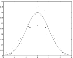
Figure 1: Distribution of 5000 values assumed by the normalized bias term (24), when $X$ has constant volatility and compound Poisson jumps (MODEL 1). The continuous line is the density of the theoretical limit law ${\cal N}(0,1)$.

MODEL 2. Let us now consider a process with jump part given by a finite activity compound Poisson process and a stochastic diffusion coefficient correlated with the Brownian motion driving $X$. We generated $N=5000$ trajectories of a process of kind

$$X_{t}=\ln(S_{t})$$

where

$$\frac{dS_{t}}{S_{t-}}=\mu dt+\sigma_{t}dW_{t}^{(1)}+dJ_{t}\quad J_{t}=\sum_{i=1}^{N_{t}}Z_{i},\quad Z_{i}\sim{\cal N}(m_{G},\nu^{2}),$$

$$\sigma_{t}=e^{H_{t}},\quad dH_{t}=-k(H_{t}-\bar{H})dt+\eta dW_{t}^{(2)},\quad d<W^{(1)},W^{(2)}>_{t}=\rho dt.$$

Note that

$$dX_{t}=(\mu-\sigma^{2}/2)dt+\sigma dW_{t}^{(1)}+\ln(1+\Delta J_{t}).$$

We chose $\mu=0$, $\lambda=4$ and a negative correlation coefficient $\rho=-0.7$; then we took $H_{0}\equiv\ln(0.3)$, $k=1$, $\bar{H}=\ln(0.25)$, $\eta=0.01$ so to ensure that a path of $\sigma$ within $[0,T]$ varies most between 0.2 and 0.4. Moreover $m_{G}=0.001$, $\nu=\sqrt{0.02}$ give relative amplitudes of the jumps of $S$ most between 0.01 and 0.20. Finally we again took $n=6000$ equally spaced observations $X_{t_{i}}$ with lag $h=\frac{1}{n}$ and $r(h)=h^{0.9}$. Figure 2 shows the distribution of the normalized bias term (23) against the asymptotic density (continuous line).

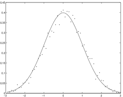
Figure 2: Distribution of 5000 values assumed by the normalized bias term (24) when $X$ has stochastic volatility, negatively correlated with $W^{(1)}$, plus compound Poisson jumps (MODEL 2). The continuous line is the density of the theoretical limit law ${\cal N}(0,1)$.

MODEL 3. Figure 3 shows the distribution obtained in the case of a Variance Gamma (VG) jump component. The VG process is a pure jump process with infinite activity and finite variation. We add to it a diffusion component $\sigma B_{t}$:

$$X_{t}=\sigma B_{t}+cG_{t}+\eta W_{G_{t}}.$$

The subordinator $G$ is a Gamma process having $Var(G_{1})=b$, $B$ and $W$ are independent Brownian motions; we chose $N=5000$, $n=6000$ and $h=1/n$. $b=0.23$, $c=-0.2$ and $\eta=0.2$ are chosen as in Madan (2001); $\sigma=0.3$ is chosen so that $Var(X_{1})=\eta^{2}+c^{2}b+\sigma^{2}=.0892$ matches the $Var(X_{1})$ we obtained for model 1. Finally $r(h)=h^{0.99}$.

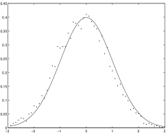
Figure 3: Distribution of 5000 values assumed by the normalized bias term (24) when $X$ has constant volatility plus a Variance Gamma jump part (MODEL 3). The continuous line is the density of the theoretical limit law ${\cal N}(0,1)$.

6 Conclusions

In this paper we devise a technique for identifying the time instants of significant jumps for a process driven by diffusion and jumps, based on a discrete record of observations, making use of a suitably defined threshold.
We provide a consistent estimate of $IV=\int_{0}^{T}\sigma^{2}_{t}dt$, extending previous results (Mancini 2001, 2004) with very mild assumptions on $a$ and $\sigma$ and, most importantly, allowing for infinite jump activity.
When $J$ has finite activity, we give a nonparametric estimate of the jump times and sizes, while when $J$ has a pure jump Lévy component with infinite activity we can identify the instants when jumps are larger than the threshold. When $J$ has FA we also prove central limit results for $\hat{IV}$ and for the jump sizes estimates.

Compared with power variations, multipower variations or kernel estimators the threshold method in the FA case is a more effective way to identify each interval $]t_{j-1},t_{j}]$ where $J$ jumped.

We also prove that the threshold estimator of $IV$ is efficient.
Moreover, our method allows the extension of kernel estimators in diffusion frameworks to processes driven by diffusions and jumps, provided we eliminate the jumps (Mancini and Renò, 2006).
The consistency of the threshold estimator holds even under leverage, both in FA and IA cases.
The threshold technique holds even when the observations are not equally spaced and also when the threshold is time varying, which is particularly important for the practical application of the estimator.

The advantage of the approach presented here is that it allows to prove a central limit theorem for $\hat{IV}$ without any substantial assumptions on $\sigma$, while in Jacod (2006) an assumption on the dynamics of $\sigma$ is needed in order to get a CLT. This topic is further developed in Cont and Mancini (2005).

The good performance of our estimator on finite samples of realistic length is shown within three different simulated models.

References

Aït-Sahalia, Y. (2004). Disentangling volatility from jumps. Journal of Financial Economics, 74, 487-528

Andersen, T.G., Bollerslev, T., Diebold, F.X. (2005). Parametriuc and nonparametric volatility measurement. In: Handbook of financial econometrics, Y. Aït-Sahalia and L.P. Hansen Eds

Bandi, F.M., and Nguyen, T.H. (2003). On the functional estimation of jump-diffusion models. Journal of Econometrics, 116, 1, pp. 293-328(36)

Barndorff-Nielsen, O.E., Gravensen, S.E., Jacod, J., Podolskij, M. and Shephard, N. (2005). A central limit theorem for realised power and bipower variation of continuous semimartingales. To appear in From Stochastic Analysis to Mathematical Finance, Festschrift for Albert Shiryaev

Barndorff-Nielsen, O.E., Shephard (2002). Econometric analysis of realized volatility and its use in estimating stochastic volatility models. Journal of the Royal Statistical Society, Series B, 64, 253-280

Barndorff-Nielsen, O.E. and Shephard, N. (2004a). Power and bipower variation with stochastic volatility and jumps (with discussion). Journal of Financial Econometrics 2, 1-48

Barndorff-Nielsen, O.E. and Shephard, N. (2004b). Econometrics of testing for jumps in financial economics using bipower variation. Journal of Financial Econometrics, 2006, 4, 1-30

Barndorff-Nielsen, O.E. and Shephard, N. (2006): Variation, jumps and high frequency data in financial econometrics. In Advanced in Economics and Econometrics. Theory and Applications, Ninth World Congress Eds Richard Blundell, Persson Torsten, Whitney K Newey, Econometric Society Monographs, Cambridge University Press

Barndorff-Nielsen, O.E., Shephard, N., Winkel, M. (2006), Limit theorems for multipower variation in the presence of jumps. Stochastic Processes and Their Applications, 2006, 116, 796-806

Berman, S.M. (1965). Sign-invariant random variables and stochastic processes with sign invariant increments. Trans. Amer. Math. Soc, 119, 216-243

Chung, K.L. (1974). A course in probability theory. Academic Press Inc.

Cont, R. and Mancini, C. (2005). Detecting the presence of a diffusion and the nature of the jumps in asset prices. Working paper

Cont, R. and Tankov, P. (2004). Financial modelling with jump processes. Chapman& Hall - CRC

Das, S. (2002). The surprise element: jumps in interest rates. Journal of Econometrics, 106, 27-65

Fan, J. (2005). A selective overview of nonparametric methods in finance. Statistical Science 20 (4), 317-337

Ikeda, N., Watanabe, S. (1981). Stochastic differential equations and diffusion processes. North Holland

Jacod, J. (2006). Asymptotic properties of realized power variations and associated functionals of semimartingales. arXiv, 20 April 2006 n. 0023146

Jacod, J., Protter, P. (1998). Asymptotic error distributions for the Euler method for stochastic differential equations. The Annals of Probability 26, 267-307

Johannes, M. (2004). The statistical and economic role of jumps in continuous-time interest rate models. The Journal of finance, 59, 227-260.

Karatzas, I., Shreve, S.E. (1999): Brownian motion and stochastic calculus. Springer

Madan, D.B. (2001) Purely discontinuous asset price processes. Advances in Mathematical Finance Eds. J. Cvitanic, E. Jouini and M. Musiela, Cambridge University Press

Mancini, C. (2001). Disentangling the jumps of the diffusion in a geometric jumping Brownian motion. Giornale dell’Istituto Italiano degli Attuari, Volume LXIV, Roma, 19-47

Mancini, C., (2004). Estimation of the parameters of jump of a general Poisson-diffusion model. Scandinavian Actuarial Journal, 2004, 1:42-52

Mancini, C., Renò, R. (2006). Threshold estimation of jump-diffusion models and interest rate modeling. working paper

Piazzesi, M. (2005). Bond Yields and the Federal Reserve. Journal of Political Economy 113 (2), 311-344

Protter, P., (1990) Stochastic integration and differential equations. Springer-Verlag

Revuz, D., Yor, M. (2001) Continuous martingales and Brownian motion. Springer

Sato, K., (1999). Lévy Processes and infinitely divisible distributions. Cambridge University Press

Woerner, J. (2006): Power and Multipower variation: inference for high frequency data. In Stochastic Finance, eds A.N. Shiryaev, M. do Rosário Grossinho, P. Oliviera, M. Esquivel, Springer, 343-364.