Variational optimization of probability measure spaces resolves
the chain store paradox

Abstract

In game theory, players have continuous expected payoff functions and can use fixed point theorems to locate equilibria. This optimization method requires that players adopt a particular type of probability measure space. Here, we introduce alternate probability measure spaces altering the dimensionality, continuity, and differentiability properties of what are now the game’s expected payoff functionals. Optimizing such functionals requires generalized variational and functional optimization methods to locate novel equilibria. These variational methods can reconcile game theoretic prediction and observed human behaviours, as we illustrate by resolving the chain store paradox. Our generalized optimization analysis has significant implications for economics, artificial intelligence, complex system theory, neurobiology, and biological evolution and development.

I Introduction

In game theory, as formalized by von Neumann and Morgenstern vonNeumann_44 , Nash Nash_50_48 ; Nash_51_28 , and Kuhn Kuhn_1953 , rational players with common knowledge of rationality (CKR) locate equilibria by using fixed point theorems to optimize continuous expected payoff functions. These expected payoff functions, according to probability measure theory Bauer_1981 ; Pfeiffer_1990 ; Kelly_94 , can only be defined after the adoption of a suitable probability measure space supporting appropriate random variables, functions, and probability distributions. For instance, mixed strategy probability measure spaces were used by von Neumann and Morgenstern vonNeumann_44 and Nash Nash_50_48 ; Nash_51_28 , while behavioural strategy probability measure spaces were introduced by Kuhn Kuhn_1953 . In addition, correlated strategy probability measure spaces were introduced by Aumann to model communication channels between players Aumann_74_67 . In this last case, communications necessitate a change of probability measure space, however a change of probability space does not always require communication. Consequently, in this paper we introduce a method to analyze games using the infinite number of different probability measure spaces available to describe any given game and set of expected payoffs Bauer_1981 ; Pfeiffer_1990 ; Kelly_94 . Our particular interest lies in the class of probability measure spaces which is consistent with the given game information constraints. That is, we consider only probability measure spaces which are consistent with rationality, CKR, and no communication channels between players. Such probability measure spaces can exist, as we show later, simply because a number of different probability measure spaces are consistent with information flow via the game history set without any communication channels. In this paper, we suppose players may freely alter their choice of probability measure space among all those consistent with no communications or any other alteration in the game, in contrast to, for instance, previous work on correlated equilibria Aumann_74_67 . For many games, a change in the underlying probability measure space will not affect equilibria—witness the equivalence of mixed and behavioural strategies in games of perfect recall Kuhn_1953 . However, in this paper, we argue that there exist games in which altering the choice of probability measure space will alter strategic equilibria. Assuming rationality, CKR, and the usual game information constraints, players can search an enlarged space of alternate probability measure spaces to optimize their expected payoffs, and thereby locate novel equilibria improving their outcomes over those achieved using only the conventional mixed or behavioural strategy probability spaces of game theory.

In this paper, we assess for the first time whether the set of equilibria of any arbitrary game are entirely invariant under the altered mathematical parameterizations defined by different probability measure spaces. It does appear that equilibria are indeed invariant under alternate probability measure spaces for single-player and multiple-player-single-stage games. However, equilibria are not invariant under altered choice of probability measure space for multiple-player-multiple-stage games. In these games, the adoption of alternate probability measure spaces by players can so alter the parameterized expected payoff functions as to generate entirely novel sets of equilibria.

Demonstrating this requires a significant generalization of the usual optimization methods of game theory. This is because alternate probability measure spaces and parameterizations can alter the functional form, dimensionality, continuity and differentiability properties of what must now be treated as expected payoff functionals (not functions). As a result, the multiple-player calculus methods (essentially fixed point theorems) suitable for expected payoff functions defined over continuous probability simplexes are insufficient. To optimize expected payoff functionals, we must generalize the variational and functional optimization techniques used in, for instance, general equilibrium and Cass-Koopmans style optimal growth analysis Cass_1965_233 ; Koopmans_1965_1 , Ramsey-style multiple stage optimization Ramsey_1928_543 ; Kamien_1991 ; Chiang_2000 , and continuous time differential games Dockner_2000 . Suitably generalized, these variational and functional optimization techniques can reconcile game theoretic prediction and observed human behaviour as we illustrate using Selton’s chain store paradox Selten_78_12 . In this game, backwards induction predicts that a monopolist never fights new market entrants even though, in practice, most monopolists will indeed fight new entrants and thereby improve their payoffs. This led Selton to conclude “mathematically trained persons recognize the logical validity of the induction argument, but they refuse to accept it as a guide to practical behavior.” Selten_78_12 . This stark contrast makes this game a suitable vehicle for the presentation of our new methods.

II Variational optimization of probability measure spaces

We consider the general strategic optimization problem faced by two players $X$ and $Y$ seeking to maximize their respected expected payoffs $\langle\Pi^{X}\rangle$ and $\langle\Pi^{Y}\rangle$ in a game where $X$ chooses events $x$ and $Y$ chooses events $y$ to generate respective payoff outcomes for each player of $\Pi^{X}(x,y)$ and $\Pi^{Y}(x,y)$. The chosen events $x\times y$ are contained in $\Omega^{X}\times\Omega^{Y}$, the set of all possible events in the game and in both player’s chosen “roulette” randomization devices. These devices are used by players to avoid their choices being forecast and exploited, with the result that the choice of events is described using a joint probability distribution $P^{XY}_{xy}$. As is required in probability measure theory Bauer_1981 ; Pfeiffer_1990 ; Kelly_94 , the definition of this joint probability distribution requires player $X$ to adopt a probability measure space ${\cal P}^{X}$, and player $Y$ to adopt a probability measure space ${\cal P}^{Y}$, such that the joint product probability measure space ${\cal P}^{X}\times{\cal P}^{Y}$ supports the probability measure $P^{XY}_{xy}$. We allow players to vary their choice of probability measure space to maximize their expected payoffs. Altogether, the strategic optimization problem facing each player is

$$X\!\!:\;\max_{{\cal P}^{X}}\;\;\langle\Pi^{X}\rangle\!\! = \!\!\int_{\Omega^{X}\!\!\times\Omega^{Y}}dP^{XY}_{xy}\;\;\Pi^{X}(x,y)$$

$$Y\!\!:\;\max_{{\cal P}^{Y}}\;\;\langle\Pi^{Y}\rangle\!\! = \!\!\int_{\Omega^{X}\!\!\times\Omega^{Y}}dP^{XY}_{xy}\;\;\Pi^{Y}(x,y).$$

Here, expected payoffs for each player $Z\in\{X,Y\}$ are defined by a Lebesgue integral over all possible game and roulette events $\Omega^{X}\times\Omega^{Y}$ of payoffs $\Pi^{Z}(x,y)$ resulting from particular game events $(x,y)$ weighted by the joint probability measure of those events occurring $P^{XY}_{xy}$. The optimization involves each player $Z$ maximizing their expected payoff over every possible joint probability measure space that might be adopted ${\cal P}^{X}\times{\cal P}^{Y}$, where ${\cal P}^{Z}=\{\Omega^{Z},\sigma^{Z},P^{Z}\}$ is defined in terms of an appropriate event set $\Omega^{Z}$ modelling all game and roulette device events, a suitable sigma-algebra $\sigma^{Z}$, and an appropriate probability measure $P^{Z}$.

Game theory has not previously allowed rational players to vary their choice of probability space to maximize their expected payoffs. This is largely because von Neumann and Morgenstern’s original goal was to formulate strategic plans assessing every possible move in a game vonNeumann_44 , and they considered this goal required only that each player adopt a particular probability measure space defining mixed strategies in any game. (Kuhn later introduced alternate behavioural strategy probability measure spaces providing an equivalent analysis in games of perfect recall Kuhn_1953 .) While never stated explicitly, this restriction essentially limits the search space of the players so they can only optimize over the probability parameters of a single type of probability space using fixed point theorems to locate Nash equilibria. In contrast, we argue that, under CKR, players can search every alternate probability space consistent with game information constraints by using generalized variational and functional optimization techniques. In the remainder of this section, we seek to explain heuristically why such a generalized analysis can generate novel and improved equilibria, and thus reconcile game theoretic prediction and observed human behaviours.

Alternate probability measure spaces can support different equilibria in strategic situations as each adopted probability space can mathematically parameterize the same random event in very different ways. For example, consider a player $X$ seeking to optimize a binary outcome specified by a random variable taking value $x=0$ with probability $P^{X}(0)$ or $x=1$ with probability $P^{X}(1)$. These probabilities can be characterized in terms of a single probability parameter $p$ by tossing a biased coin, or in terms of five probability parameters $(p_{1},p_{2},p_{3}.p_{4},p_{5})$ say by using a biased dice. An alternative probability measure space might employ two sequentially tossed, independent, biased coins producing outcomes $u=1$ with probability $p$, while if $u=0$ then $v=1$ with probability $q$ and if $u=1$ then $v=1$ with probability $r$. The subsequent adoption of the random variable $x=\delta_{u1}\delta_{v1}$ defines $P^{X}(1)=P(u=1,v=1)=pr$. (Here, $\delta_{ab}=1$ if $a=b$ and zero otherwise.) As a last illustration, consider a probability measure space in which the above two biased coins are now perfectly correlated via $P(u,v)=P(u)P(v|u)=P(u)\delta_{uv}=P(u)$. In this case, the known perfect correlation introduces a delta function to reduce the dimensionality of the joint distribution $P(u,v)$ giving $P^{X}(1)=P(u=1,v=1)=p$. In general, when parameterized using different probability measure spaces, a given probability possesses alternate functional forms with different dimensionality, correlation, continuity, and differentiability properties.

This changeability of functional form and dimensionality requires generalized variational and functional optimization methods be used to optimize strategic decisions. The generalized methods we develop extend the calculus of variations which typically optimizes a functional $F[f(x),f^{\prime}(x)]$ of known form, and where the functional $F$, the function $f(x)$, and the gradient $f^{\prime}(x)$ have specified differentiability properties. For instance, a shortest path problem seeks to optimize the known functional $F[f(x),f^{\prime}(x)]=\sqrt{1+f^{\prime 2}}$ via

$$\max_{f,f^{\prime}}\;\;I=\int_{a}^{b}\sqrt{1+f^{\prime 2}}dx.$$ (2)

Similarly, the shortest time or Brachistochrone problem optimizes the known functional $F[f(x),f^{\prime}(x)]=\sqrt{\frac{1+f^{\prime 2}}{2gf}}$ via

$$\max_{f,f^{\prime}}\;\;I=\int_{a}^{b}\sqrt{\frac{1+f^{\prime 2}}{2gf}}dx.$$ (3)

Lastly, a typical multiple stage Ramsey-style utility maximization problem optimizes

$$\max_{f,f^{\prime}}\;\;I=\int_{a}^{b}e^{-rx}F[f-f^{\prime}]dx,$$ (4)

where now only the functional dependencies and certain differentiability properties of the functional $F[f(x),f^{\prime}(x)]$ are specified. To our knowledge, all applications of the calculus of variations place severe restrictions on the range of variation of the form of the functional being optimized, so much so that a problem with an entirely arbitrary functional would be considered ill defined. In contrast, in a strategic optimization problem, players are able to arbitrarily vary their choice of probability measure space to alter all of the functional form, the dimensionality, and the continuity and differentiability properties of the functional being optimized. Heuristically, in single player terms, the optimization problem becomes

$$\max_{f,f^{\prime}}\;\;I=\left\{\begin{array}[]{c}\vdots\\ \\ \int_{a}^{b}\sqrt{1+f^{\prime 2}}dx\\ \\ \int_{a}^{b}\sqrt{\frac{1+f^{\prime 2}}{2gf}}dx\\ \\ \int_{a}^{b}e^{-rx}F[f-f^{\prime}]dx\\ \\ \vdots\\ \end{array}\right..$$ (5)

That is, each player has the option of first choosing a parameterizing probability measure space to alter the functional form, dimensionality, continuity and differentiability properties of the functionals being optimized, and only then to optimize the chosen functional over all possible variations of $f(x)$ and $f^{\prime}(x)$. More importantly, each of their choices affects their opponent’s functionals, while at the same time, their opponent’s decisions are similarly altering their own functionals.

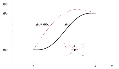
Figure 1: The variational optimization of the functional $F[f(x),f^{\prime}(x)]$ requires the variation of both the function $f(x)\rightarrow f(x)+\delta f(x)$ and independently, its gradient $f^{\prime}(x)\rightarrow f^{\prime}(x)+\delta f^{\prime}(x)$ over the region $[a,b]$. That is, through any point “$A$”, every possible gradient must be considered in order to perform a complete variational analysis.

We suggest that this variability of the strategic functionals means that optimization requires independent examination of every possible functional, and every possible functional gradient, that might be defined by the players. That is, we generalize the standard optimization algorithm of the calculus of variations in which functionals $F[f(x),f^{\prime}(x)]$ of known form are optimized by an independent variation of the function $f$ and the gradient $f^{\prime}$. This independent variation of each of the coordinates $(f,f^{\prime})$ over every possible value allows for instance, derivation of the Euler-Lagrange equations providing the first order optimization conditions. This is depicted in Fig. 1 showing that every possible gradient and trajectory through any point “A” in the parameter space must be considered to locate optimal trajectories. Any restrictions on this search of all possible trajectories constrains the optimization. For instance, when players are restricted to using only a particular type of probability measure space, i.e. mixed or behavioural strategy spaces, then expected payoff functions have fixed functional form, are continuous, and possess a single gradient at every point in the joint function space. These restrictions allow use of the calculus (effectively fixed point theorems) rather than a generalized calculus of variations to locate equilibria.

We argue that, under CKR, players should potentially benefit from the ability to search an enlarged mathematical space including many alternative joint probability measure spaces. A complete search of this enlarged mathematical space requires that they examine not only every possible value of the expected payoff functions at every point in their parameter space, but also every possible gradient at every one of those points. In the following, we show that different probability measure spaces can associate different gradients with the same point in the joint expected payoff function space, and we argue that every such possible gradient must be taken into account in any complete variational and functional optimization. That is, when players $X$ and $Y$ are seeking to optimize their respective expected payoffs $\langle\Pi^{X}\rangle$ and $\langle\Pi^{Y}\rangle$, they must examine not only every possible pair of joint values $\left(\langle\Pi^{X}\rangle,\langle\Pi^{Y}\rangle\right)$ but also every possible joint gradient $\left(\frac{\partial\langle\Pi^{X}\rangle}{\partial p_{1}},\frac{\partial\langle\Pi^{X}\rangle}{\partial p_{2}},\dots,\frac{\partial\langle\Pi^{Y}\rangle}{\partial q_{1}},\frac{\partial\langle\Pi^{Y}\rangle}{\partial q_{2}},\dots\right)$ evaluated with respect to every possible parameterization $(p_{1},p_{2},\dots,q_{1},q_{2},\dots)$ defined in every possible joint probability measure space.

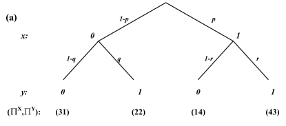
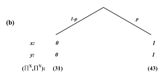
Figure 2: A simple example two-player-two-stage perfect information game showing the different game decision trees specific to players adopting the respective joint probability spaces (a) ${\cal P}^{X}_{0}\times{\cal P}^{Y}_{0}$ where optimal player choices are $(x,y)=(0,1)$ generating expected payoffs $\left(\langle\Pi^{X}\rangle,\langle\Pi^{Y}\rangle\right)=(2,2)$, and (b) ${\cal P}^{X}_{0}\times{\cal P}^{Y}_{1}$ where optimal player choices are $(x,y)=(1,1)$ generating expected payoffs $\left(\langle\Pi^{X}\rangle,\langle\Pi^{Y}\rangle\right)=(4,3)$.

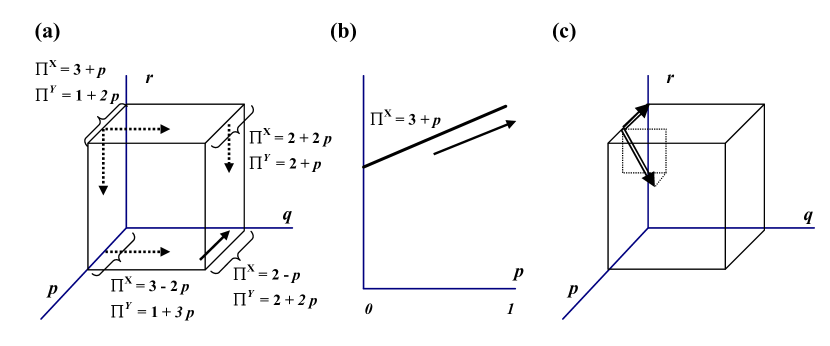
Figure 3: (a) Game theory adopts a joint probability measure space ${\cal P}^{X}_{0}\times{\cal P}^{Y}_{0}$ in which expected payoffs vary over three dimensions $(p,q,r)$ and where positive gradients with respect to $q$ and $r$ (dotted arrows) and with respect to $p$ (solid arrow) ensure that players maximize joint payoffs by choosing $(p,q,r)=(0,1,0)$. (b) An alternate joint probability space ${\cal P}^{X}_{0}\times{\cal P}^{Y}_{1}$ in which expected payoffs vary solely over a single dimension $p$ with positive gradients with respect to $p$ (solid arrow) ensuring that players optimize payoffs by choosing $p=1$. (c) The choice of two alternate probability spaces (more are possible) associates two different total gradients (double-lined arrows) with any point along the perfect correlation line $\rho_{xy}=1$ at $(q,r)=(0,1)$ with $\left.\left(\frac{\partial\langle\Pi^{X}_{00}(p,q,r)\rangle}{\partial p},\frac{\partial\langle\Pi^{Y}_{00}(p,q,r)\rangle}{\partial q},\frac{\partial\langle\Pi^{Y}_{00}(p,q,r)\rangle}{\partial r}\right)\right|_{(q,r)\rightarrow(0,1)}\neq\left(\frac{\partial\langle\Pi^{X}_{01}(p)\rangle}{\partial p}\right)$. In the absence of any effective decision procedure privileging any one space over another, players should examine all possible spaces, all possible gradients, and all possible trajectories.

III Variational optimization in multiple stage games

In this section, we use a simple two-player-two-stage game to introduce standard mathematical methods that have not previously been applied in game analysis. Our goal is to demonstrate that even simple games can exhibit expected payoffs with multiple functional forms, multiple gradients and multiple trajectories at the same point in the parameter space necessitating use of variational optimization methods.

Suppose two players, denoted $Z\in\{X,Y\}$, each seek to optimize their own outcomes in a strategic interaction, where in stage one $X$ makes a choice of $x=0$ or $x=1$. In the second stage, player $Y$ is aware of the opponent’s previous choice and must also make a choice of $y=0$ or $y=1$ at which point the game terminates and players obtain payoffs $\Pi^{Z}(x,y)$ as shown in Fig. 2(a).

Game theory analyzes this game by having each player adopt a joint probability space allowing the complete analysis of every possible choice that might be made in the game. In this game, both players suppose that $X$ adopts a probability space ${\cal P}^{X}_{0}$ with random variable $x\in\{0,1\}$ taking value $x=1$ with probability $p$. In turn, both players suppose that player $Y$ chooses a probability space allowing for any degree of correlation $\rho$ between the observable game events $x$ and $y$, that is, that these variables might be perfectly correlated $\rho_{xy}=1$, or perfectly anti-correlated $\rho_{xy}=-1$, or entirely uncorrelated $\rho_{xy}=0$, or any value in between. Player $Y$ does this by adopting the probability space ${\cal P}^{Y}_{0}$ with random variables $y,u,v\in\{0,1\}$ with $u$ and $v$ independent and taking values $u=1$ with probability $q$ and $v=1$ with probability $r$. The random variable $y$ is functional determined to be

$$y=\left\{\begin{array}[]{cc}u&\mbox{if }x=0\\ &\\ v&\mbox{if }x=1,\\ \end{array}\right.$$ (6)

giving

$$P^{Y}(y|x)=\left\{\begin{array}[]{l}P^{Y}(0|0)=1-q\\ \\ P^{Y}(1|0)=q\\ \\ P^{Y}(0|1)=1-r\\ \\ P^{Y}(1|1)=r\\ \end{array}\right..$$ (7)

As desired, this choice of probability space allows the players to examine every possible correlation state between $x$ and $y$ defined as

$$\rho_{xy}(p,q,r) = \frac{\langle xy\rangle-\langle x\rangle\langle y\rangle}{\sqrt{\langle x^{2}\rangle-\langle x\rangle^{2}}\sqrt{\langle y^{2}\rangle-\langle y\rangle^{2}}}$$ (8)

$$= \frac{\sqrt{p(1-p)}(r-q)}{\sqrt{\left[q+p(r-q)\right]\left[1-q-p(r-q)\right]}}.$$

Then, $x$ and $y$ are perfectly correlated at $\rho_{xy}(p,0,1)=1$, perfectly anti-correlated at $\rho_{xy}(p,1,0)=-1$, and uncorrelated if either $p=0$ or $1$ or $q=r$ giving $\rho_{xy}=0$. As shown in Fig. 3(a), in the joint probability space ${\cal P}^{X}_{0}\times{\cal P}^{Y}_{0}$, the expected payoff functions are

$$\langle\Pi^{X}_{00}(p,q,r)\rangle = \sum_{xy=0}^{1}P^{X}(x)P^{Y}(y|x)\Pi^{X}(x,y)$$

$$= 3-q+p(q+3r-2)$$

$$\langle\Pi^{Y}_{00}(p,q,r)\rangle = \sum_{xy=0}^{1}P^{X}(x)P^{Y}(y|x)\Pi^{Y}(x,y)$$ (9)

$$= 1+q-p(q+r-3),$$

so the gradients with respect to the three continuous dependent variables $p$, $q$ and $r$ are

$$\frac{\partial\langle\Pi^{X}_{00}(p,q,r)\rangle}{\partial p} = q+3r-2$$

$$\frac{\partial\langle\Pi^{Y}_{00}(p,q,r)\rangle}{\partial q} = 1-p$$

$$\frac{\partial\langle\Pi^{Y}_{00}(p,q,r)\rangle}{\partial r} = -p.$$ (10)

As shown in Fig. 3(a), this three-dimensional gradient exists and is non-zero even when $x$ and $y$ are perfectly correlated $\rho_{xy}=1$ at all points $(q,r)=(0,1)$ so payoffs are not optimized at these points. In fact, given the choice of probability space ${\cal P}^{X}_{0}\times{\cal P}^{Y}_{0}$, both players conclude that $Y$ maximizes their payoff by setting $(q,r)=(1,0)$ while $X$ maximizes their payoff by setting $p=0$. The resulting move choices are $(x,y)=(0,1)$ generating payoffs of $\left(\langle\Pi^{X}\rangle,\langle\Pi^{Y}\rangle\right)=(2,2)$. This completes our analysis of the usually adopted joint probability measure space, and we now turn to examine alternatives.

In any game, alternate joint probability measure spaces exist with expected payoff functions of different functional form and different gradients at the same point in the parameter space. Suppose that player $Y$ chooses a different probability space ${\cal P}^{Y}_{1}$ in which they treat the observed value of the random variable $x$ as a coin toss determining their choice of $y=1$ with probability $p$. That is, $Y$ functionally assigns the random variable $y$ to be perfectly correlated with the observed random variable $x$ via

$$y = x$$

$$P^{Y}(y|x) = \delta_{yx}.$$ (11)

This functional assignment does not require any communication between player $X$ and $Y$. Then, in the joint probability space ${\cal P}^{X}_{0}\times{\cal P}^{Y}_{1}$, the expected payoff functions straightforwardly equal

$$\langle\Pi^{X}_{01}(p)\rangle = \sum_{xy=0}^{1}P^{X}(x)P^{Y}(y|x)\Pi^{X}(x,y)$$

$$= 3+p$$

$$\langle\Pi^{Y}_{01}(p)\rangle = \sum_{xy=0}^{1}P^{X}(x)P^{Y}(y|x)\Pi^{Y}(x,y)$$ (12)

$$= 1+2p,$$

as seen in the decision tree of Fig. 2(b), and in the expected payoff function space of Fig. 3(b). These expected payoff functions are now dependent only on the single freely varying parameter $p$ determining the gradient with respect to $p$ to be

$$\frac{\partial\langle\Pi^{X}_{01}(p)\rangle}{\partial p}=1.$$ (13)

Consequently, player $X$ maximizes their payoff by setting $p=1$ to choose $x=1$ leading $Y$ to set $y=1$. Thus, in the joint probability space ${\cal P}^{X}_{0}\times{\cal P}^{Y}_{1}$, player payoffs are $\left(\langle\Pi^{X}\rangle,\langle\Pi^{Y}\rangle\right)=(4,3)$.

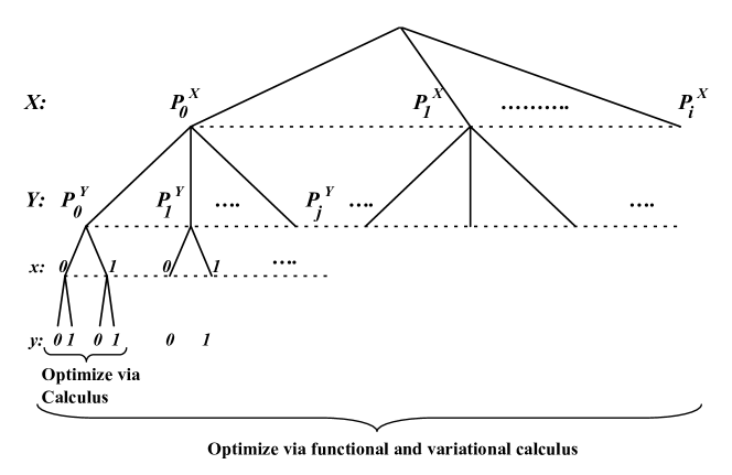
Figure 4: A schematic representation of a complete analysis of the simple game of Fig. 2 showing that each player must first decide which probability space to adopt. Here, players $X$ and $Y$ simultaneously choose their respective probability spaces ${\cal P}^{X}_{i}$ and ${\cal P}^{Y}_{j}$ from among an infinite number of possibilities, where each choice generates a different decision tree for the game defining altered payoff functions. Players do not know their opponent’s choice of probability space. Given the adoption of a particular joint probability space ${\cal P}^{X}_{i}\times{\cal P}^{Y}_{j}$, expected payoff functions are known and continuous in terms of their input parameters so the calculus, suitably generalized for multiple-player strategic interactions, can be used to optimize payoffs. However, optimizing the choice of joint probability space involves expected payoff functionals requiring players to use variational calculus methods to optimize payoffs.

We now have two possible joint probability spaces; that normally adopted in game theory ${\cal P}^{X}_{0}\times{\cal P}^{Y}_{0}$ and the novel ${\cal P}^{X}_{0}\times{\cal P}^{Y}_{1}$. In these alternate spaces, the expected payoff functions possess exactly the same value when $x$ and $y$ are perfectly correlated but possess entirely different gradients at this point—see Fig. 3(c). Variational optimization principles insist that every possible functional form and gradient must be taken into account in any complete optimization. These principles permit players to infinitely vary the “immutable” functional assignments defining any space (i.e. $y=\delta_{x0}u+\delta_{x1}v$ and $y=x$ above), providing access to a vastly larger decision space than usually analyzed in game theory. It is not a question of which space is best, rather, it is a question of either restricting the analysis to a single space or allowing players to analyze all possible spaces.

Game theory adopts expected payoff “functions” $\langle\Pi^{Z}_{00}(p,q,r)\rangle$ allowing examination of every possible combination of payoff values and assumes that this is sufficient for optimization. However, while these functions can duplicate every possible payoff value, they cannot duplicate every possible functional gradient—and optimization depends on gradients. When $Y$ adopts a randomization device (a “roulette”) which perfectly correlates $x$ and $y$ via the probability space ${\cal P}^{Y}_{1}$, then certainly $\langle\Pi^{Z}_{00}(p,0,1)\rangle=\langle\Pi^{Z}_{01}(p)\rangle$, but these functions have different dimensionality and gradients. That is, $\left.\left(\frac{\partial\langle\Pi^{X}_{00}(p,q,r)\rangle}{\partial p},\frac{\partial\langle\Pi^{Y}_{00}(p,q,r)\rangle}{\partial q},\frac{\partial\langle\Pi^{Y}_{00}(p,q,r)\rangle}{\partial r}\right)\right|_{(q,r)\rightarrow(0,1)}\neq\left(\frac{\partial\langle\Pi^{X}_{01}(p)\rangle}{\partial p}\right)$. Similar results apply for points at different correlation values $\rho_{xy}$; should $Y$ adopt a randomization device where $y$ is entirely uncorrelated with $x$ via a new probability space ${\cal P}^{Y}_{2}$, then certainly $\langle\Pi^{Z}_{00}(p,q,q)\rangle=\langle\Pi^{Z}_{02}(p,q)\rangle$ but these functions again have different dimensionality and gradients $\left.\left(\frac{\partial\langle\Pi^{X}_{00}(p,q,r)\rangle}{\partial p},\frac{\partial\langle\Pi^{Y}_{00}(p,q,r)\rangle}{\partial q},\frac{\partial\langle\Pi^{Y}_{00}(p,q,r)\rangle}{\partial r}\right)\right|_{r=q}\neq\left(\frac{\partial\langle\Pi^{X}_{02}(p,q)\rangle}{\partial p},\frac{\partial\langle\Pi^{Y}_{02}(p,q)\rangle}{\partial q}\right)$. These inequalities result as the usually adopted space ${\cal P}^{X}_{0}\times{\cal P}^{Y}_{0}$ evaluates gradients using infinitesimals between points with different correlations so $\Delta\rho_{xy}=\rho_{xy}(p,q,r)-\rho_{xy}(p+\delta p,q+\delta q,r+\delta r)\neq 0$. In contrast, when a roulette possesses a known correlation state as in the spaces ${\cal P}^{X}_{0}\times{\cal P}^{Y}_{1}$ or ${\cal P}^{X}_{0}\times{\cal P}^{Y}_{2}$, then gradients are evaluated taking all constraints into account ensuring $\Delta\rho_{xy}=0$. Game analysis does not include every possible correlation constraint or every possible roulette, and taking these alternatives into account requires the variational methods presented in this paper.

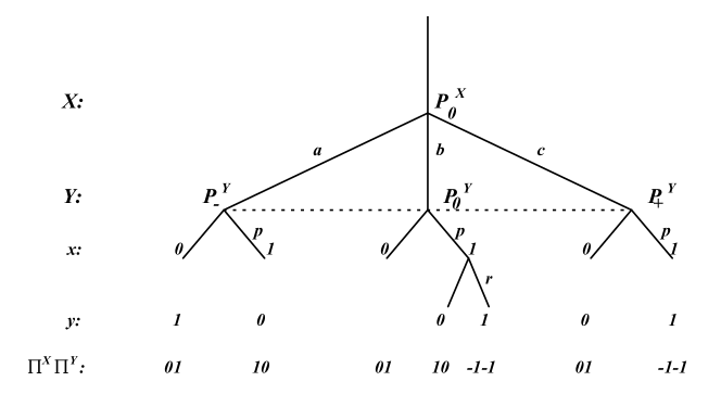
Figure 5: An extended decision tree for the chain store paradox where player $X$ adopts the usual probability space ${\cal P}^{X}_{0}$ with certainty while $Y$ has a choice of three alternate probability spaces ${\cal P}^{Y}_{j}$ for $j\in\{-,0,+\}$ selected with probabilities $a$, $b$, and $c$, and respectively denoting anti-correlated, independent, and correlated decision making. Game theory examines only the branch generated by the joint probability space ${\cal P}^{X}_{0}\times{\cal P}^{Y}_{0}$ in which a potential new market entrant $X$ must decide to either stay out of a new market $x=0$ or enter the market $x=1$ (with probability $p$), in which case the monopolist $Y$ chooses to either acquiesce $y=0$ or fight their entry $y=1$ (with probability $r$), with the corresponding payoffs shown.

We suggest that the example game described in the two decision trees of Fig. 2 is best seen as having the schematic form shown in Fig. 4 in which players must first choose which probability space they will adopt, where this choice is unknown to their opponents at the commencement of the game, and must then optimize their payoffs given the possible joint probability spaces that might be adopted. In such generalized trees incorporating choice of probability space, standard approaches can be applied to locate pure “variational” strategies, probabilistic “variational” mixed and “variational” behavioural strategies, and “variational” equilibria. Of course, introducing “variational” mixed and behavioural strategies means that players must introduce yet further probability spaces allowing the optimization of these probabilistic strategies.

To provide a concrete illustration of our approach, we now show that rational players using variational optimization methods can resolve the chain store paradox.

IV Resolving the chain store paradox

A minimal chain store paradox is shown as the central branch in Fig. 5 generated by the adoption of the joint probability space ${\cal P}^{X}_{0}\times{\cal P}^{Y}_{0}$ (defined below). This game is played over two sequential stages where first, a potential market entrant $X$ must decide to either stay out of a new market $x=0$ or enter that market $x=1$. Their opponent, the monopolist $Y$, observes this choice. Should no market entry occur, $X$ neither gains nor loses any payoff while $Y$ gains monopolist profits so $(\Pi^{X},\Pi^{Y})=(0,1)$. In contrast, should $X$ enter the market, $Y$ must then decide whether to acquiesce to their opponent’s entry $y=0$ by leaving prices unchanged and sharing profits so $(\Pi^{X},\Pi^{Y})=(1,0)$, or by driving $X$ out of business by price cutting so payoffs are $(\Pi^{X},\Pi^{Y})=(-1,-1)$.

A backwards induction analysis of the central branch of Fig. 5 in isolation indicates that $X$ will enter the market confident that the monopolist will not forego profits to fight their entry Selten_78_12 . Based on this, many economists argue it is irrational for monopolists to engage in predatory pricing to drive rivals out of business as predation is costly while potential new entrants well understand that price cuts are temporary and monopoly profits readily attract new market entrants Milgrom_1982_280 . Efforts to resolve the paradox include introducing multiple stages permitting reputation and deterrence effects Selten_78_12 , as well as asymmetric information, mistakes, bounded rationality or imperfect information and uncertainty Milgrom_1982_280 ; Rosenthal_1981_92 ; Davis_85_13 ; Kreps_1982_253 ; Trockel_86_16 . For a review, see Wilson_1992_305 .

The decision and payoff combinations above define the general strategic optimization problem faced by the players in the chain store paradox as

$$X\!\!:\max_{{\cal P}^{X}}\;\;\langle\Pi^{X}\rangle = P^{X}(1)\left[1-2P^{Y}(1|1)\right]$$

$$Y\!\!:\max_{{\cal P}^{Y}}\;\;\langle\Pi^{Y}\rangle = 1-P^{X}(1)-P^{X}(1)P^{Y}(1|1).$$

Here, players alter their choice of joint probability space ${\cal P}^{X}\times{\cal P}^{Y}$ such that, within the selected optimal joint probability space, the optimization of their respective probability distributions $P^{X}(x)$ and $P^{Y}(y|x)$ allows optimal choices $(x,y)$ to be made so as to maximize respective payoffs.

A complete derivation of the “variational” equilibria of the extended tree of Fig. 5 is of course possible (and indicates that as long as $Y$ sets $c+br\geq\frac{1}{2}$, most easily achieved by choosing $c=1$, then $X$ maximizes their payoff through the choice $p=0$). In this paper, we locate pure variational equilibria in the chain store game. That is, we suppose that player $X$ always chooses ${\cal P}^{X}_{0}$ (other choices are possible) while player $Y$ chooses with certainty any of the three probability spaces ${\cal P}^{Y}_{j}$ with $j\in\{-,0,+\}$. The interpretation of these latter spaces is that $j=$“$-$” indicates that $y$ is perfectly anti-correlated to $x$, $j=$“$0$” indicates that $y$ is entirely independent, and $j=$“$+$” indicates that $y$ is perfectly correlated to $x$—see Fig. 5.

First, we replicate the usual game analysis by supposing that player $X$ adopts a probability space ${\cal P}^{X}_{0}$ with random variable $x\in\{0,1\}$ such that $x=1$ with probability $p$, while player $Y$ adopts the probability space ${\cal P}^{Y}_{0}$ with random variables $y,u,v\in\{0,1\}$ such that $u$ and $v$ are independent random variables taking value $u=1$ with probability $q$ and $v=1$ with probability $r$, and where the random variable $y$ is functionally assigned as $y=\delta_{x0}u+\delta_{x1}v$. Altogether, this gives the same probability parameterization for $P^{Y}(y|x)$ as appears in Eq. 7. In the joint probability space ${\cal P}^{X}_{0}\times{\cal P}^{Y}_{0}$, the optimization problem reduces to

$$X\!\!:\max_{p}\;\;\langle\Pi^{X}_{00}\rangle = P^{X}(1)\left[1-2P^{Y}(1|1)\right]$$

$$= p(1-2r)$$

$$Y\!\!:\max_{r}\;\;\langle\Pi^{Y}_{00}\rangle = 1-P^{X}(1)-P^{X}(1)P^{Y}(1|1)$$

$$= 1-p-pr,$$

so the gradients with respect to the two continuous dependent variables $p$ and $r$ are

$$\frac{\partial\langle\Pi^{X}_{00}\rangle}{\partial p} = 1-2r$$

$$\frac{\partial\langle\Pi^{Y}_{00}\rangle}{\partial r} = -p.$$ (16)

Essentially then, the monopolist $Y$ maximizes their expected payoff by setting $r=0$ and always acquiesces to new market entrants, while $X$ maximizes their payoff by choosing $p=1$ and so always decides to enter the market. The resulting expected payoffs given that players adopt this sole perfect Nash equilibria of $(p,r)=(1,0)$ are $\left(\langle\Pi^{X}\rangle,\langle\Pi^{Y}\rangle\right)=(1,0)$.

Suppose however that players $X$ and $Y$ choose the joint probability space ${\cal P}^{X}_{0}\times{\cal P}^{Y}_{+}$ (the rightmost branch of Fig. 5) where $y$ is perfectly correlated with $x$ via the functional assignment $y=x$ and $P(y|x)=\delta_{yx}$ altering the strategic optimization problem to

$$X\!\!:\max_{p}\;\;\langle\Pi^{X}_{0+}\rangle = P^{X}(1)\left[1-2P^{Y}(1|1)\right]$$

$$= -p$$

$$Y\!\!:\langle\Pi^{Y}_{0+}\rangle = 1-P^{X}(1)-P^{X}(1)P^{Y}(1|1)$$

$$= 1-2p.$$

These expected payoff functions are continuous over the single freely varying parameter $p$ giving the gradient

$$\frac{\partial\langle\Pi^{X}_{0+}\rangle}{\partial p}=-1<0$$ (18)

ensuring that player $X$ maximizes their expected payoff by setting $p=0$ and not entering the market. That is, when players $(X,Y)$ adopt the ${\cal P}^{X}_{0}\times{\cal P}^{Y}_{+}$ joint probability space, they maximize their payoffs via the combination $(x,y)=(0,0)$ to garner payoffs $\left(\langle\Pi^{X}\rangle,\langle\Pi^{Y}\rangle\right)=(0,1)$.

Alternatively, in the anti-correlated joint probability space ${\cal P}^{X}_{0}\times{\cal P}^{Y}_{-}$ (the leftmost branch of Fig. 5), $y$ is perfectly anti-correlated with $x$ via $y=(1-x)$ and $P(y|x)=\delta_{y(1-x)}$ giving the altered strategic optimization problem of

$$X\!\!:\max_{p}\;\;\langle\Pi^{X}_{0-}\rangle = P^{X}(1)\left[1-2P^{Y}(1|1)\right]$$

$$= p$$

$$Y\!\!:\langle\Pi^{Y}_{0-}\rangle = 1-P^{X}(1)-P^{X}(1)P^{Y}(1|1)$$

$$= 1-p.$$

Again, these are functions of the sole parameter $p$ giving the gradients

$$\frac{\partial\langle\Pi^{X}_{0-}\rangle}{\partial p}=1>0,$$ (20)

ensuring that player $X$ sets $p=1$ and chooses to enter the market. The result is that when players $(X,Y)$ adopt the ${\cal P}^{X}_{0}\times{\cal P}^{Y}_{-}$ joint probability space, they maximize their payoffs via the combination $(x,y)=(1,0)$ to garner payoffs $\left(\langle\Pi^{X}\rangle,\langle\Pi^{Y}\rangle\right)=(1,0)$.

Altogether, when players consider only pure variational strategies (specifying probability spaces and move choices), the various payoffs available are

$$\begin{array}[]{c|c}\left(\langle\Pi^{X}\rangle,\langle\Pi^{Y}\rangle\right)&{\cal P}^{X}_{0}\\ \hline\cr&\\ {\cal P}^{Y}_{-}&(1,0)\\ &\\ {\cal P}^{Y}_{0}&(1,0)\\ &\\ {\cal P}^{Y}_{+}&(0,1),\\ \end{array}$$ (21)

making it evident that to maximize their expected payoff, player $Y$ must rationally elect to use probability space ${\cal P}^{Y}_{+}$ in preference to either ${\cal P}^{Y}_{0}$ or ${\cal P}^{Y}_{-}$. That is, $Y$ will undertake to functionally correlate their move to the previous choice of the potential market entrant, and thereby deny themselves a choice about the setting of $y$ once the game has commenced. In the probability space ${\cal P}^{Y}_{+}$, the optimization by player $Y$ has no second stage component as the joint probability distributions are inseparable, and an opportunity for a second stage optimization exist only in the space ${\cal P}^{Y}_{0}$. Player $Y$ foregoes a choice during the game itself knowing this to be payoff maximizing. Player $X$, being aware of this will not enter the market as in the minimal chain store game described by ${\cal P}^{X}_{0}\times{\cal P}^{Y}_{+}$, entry automatically invokes retaliation. We thus reconcile game theoretic prediction and observed human behaviour implying human players generally commence a strategic analysis by first optimizing their choice of probability space and only subsequently optimizing the probability distributions defined by that space.

It is of course possible to consider a broader range of joint probability spaces for both players $X$ and $Y$, though this will not substantially alter the conclusion here that it can be rational for a monopolist to punish market entrants to resolve the chain store paradox.

V Conclusion

This paper locates strategic equilibria using generalized calculus of variation techniques and is thus consistent with, and extends, the more usual methods of game theory based on the fixed point theorems of the calculus Hart_92_19 ; Sorin_92_c4 . We hold that under CKR, players might often improve their outcomes by expanding their mathematical search space to include alternate probability spaces. Consequently, we allow players to first optimize their choices of probability measure space which alters both the expected payoff functionals (not functions) and the joint probability distributions specifying move choices to locate “variational” equilibria. Generally, these variational equilibria differ from Nash equilibria even in perfect information games such as the chain store paradox considered here. This is because first, players are uncertain about which joint probability measure space is in play, and second, each alternative space introduces different correlations rendering the joint probability distribution inseparable and altering allowable subgame decompositions and the backwards induction analysis. We show that when rational players variationally optimize their choice of probability measure space to access “variational” equilibria, then this can reconcile game theoretic prediction and observed human behaviour. To illustrate this, we demonstrated that our general variational and functional optimization approaches resolve the chain store paradox. This strongly suggests that rational players should, in fact, exploit unrestricted optimization in general.

More generally, we suggest that selfish “homo economicus” might exploit variational optimization to access alternate probability measure spaces to exhibit altruistic or cooperative behaviour whenever that is payoff-maximizing. This might explain for instance, the efficacy of state led development processes World_Bank_93 ; Stiglitz_00 and the industry wide correlations of the “Just-In-Time” Toyota production system Lu_89 ; Womack_1990 . Consequently, variational optimization may change the orientation and methods of evolutionary game theory Maynard_Smith_1982 and quantum game theory Meyer_99_10 , among other fields, while the need to search infinite numbers of joint probability spaces will reinforce the importance of learning, a principal feature of evolutionary economics Wit_1993 . Similarly, variational optimization will impact “selfish gene” theory which presently holds that genes optimize their fitness independently so altruism is explained by relatedness and the likelihood of shared genes Dawkins_1976 . In contrast, we suggest that modelling the evolution of emergent hierarchical complexity in living organisms requires taking account of alternative probability spaces correlating system components; correlated entities together constitute an indivisible unit which must be optimized as a whole. Consequently, complex multicellular eukaryotes might well have optimized fitness by adopting correlating signals to multitask their dynamics by exploring alternate dynamical decision trees (organismal probability spaces) most likely by expansion of their RNA signaling capabilities Mattick_94_823 ; Mattick_02_1611 ; Mattick_04_316 . Similar considerations mean that neural networks can endogenously modify correlations among their components to explore an infinite number of alternate dynamical trees to implement complex cognition. Game analysis also underlies the tree search “minimax” algorithms of artificial intelligence Hart_92_c2 ; Russell_2003 ; Callan_2003 which typically fail to emulate human intelligence. In chess playing, for instance, expert human players typically employ pattern recognition and “chunking” Luger_1998 , and appear to be exploiting the same correlation information that underpins variational optimization. This is consistent with the “social intelligence” explanation for the runaway evolution of primate intelligence where individuals dynamically realign their strategic partnerships to correlate behaviours to optimize outcomes in competitive group settings Byrne_1988 ; Rifkin_1995 .

It has long been thought that any strategic optimization problem was essentially equivalent to a possibly greatly enlarged non-strategic optimization problem. This equivalence arises as each player can introduce sufficient new variables to fully model all of the possible actions of all of their opponents. As a result, strategic optimization has been thought to be of equivalent complexity to, for instance, non-strategic physics optimization problems, and solved by similar methods such as the calculus of variations or the calculus. Some have argued the converse. A perceived fundamental incompatibility between physics and biological complexity motivated Mayr to claim that biology is an autonomous science rather than a subbranch of the physical sciences Mayr_2004 , with the factor missing in physics but present in biology being identified as “entailment” (essentially correlation) by Rosen Rosen_1991 , while it has been unconventionally argued that information science is incomplete and that it is our growing understanding of genomic programming and biological complexity that will contribute significant new insights in this field (J. S. Mattick, personal communication). Variational optimization might well help close these perceived gaps.

References

- (1) J. von Neumann and O. Morgenstern. Theory of Games and Economic Behavior. Princeton University Press, Princeton, 1944. Page numbers from 1953 edition.
- (2) J. F. Nash. Equilibrium points in -person games. Proceedings of the National Academy of Sciences of the United States of America, 36(1):48–49, 1950.
- (3) J. Nash. Non-cooperative games. Annals of Mathematics, 54(2):286–295, 1951.
- (4) H. W. Kuhn. Extensive games and the problem of information. In H. W. Kuhn and A. W. Tucker, editors, Contributions to the Theory of Games, Volume II, Princeton Annals of Mathematical Studies, No. 28, Princeton, 1953. Princeton University Press.
- (5) H. Bauer. Probability Theory and Elements of Measure Theory. New York, Academic Press, 1981.
- (6) P. E. Pfeiffer. Probability for Application. Springer, New York, 1990.
- (7) D. G. Kelly. Introduction to Probability. Macmillan, New York, 1994.
- (8) R. J. Aumann. Subjectivity and correlation in randomized strategies. Journal of Mathematical Economics, 1:67–96, 1974.
- (9) D. Cass. Optimal growth in an aggregate model of capital accumulation. Review of Economic Studies, 32:233–240, 1965.
- (10) T. C. Koopmans. On the concept of optimal economic growth. Pontificiae Academiae Scientiarum Scripta Varia, 28:1, 1965.
- (11) F. P. Ramsey. A mathematical theory of savings. Economic Journal, 38(152):543–559, 1928.
- (12) M. I. Kamien and N. L. Schwartz. Dynamic Optimization: The Calculus of Variations and Optimal Control in Economics and Management. North-Holland, Amsterdam, 1991.
- (13) A. C. Chiang. Elements of Dynamic Optimization. Waveland Press, Prospect Heights, 2000.
- (14) E. J. Dockner, S. Jørgensen, N. V. Long, and G. Sorger. Differential Games in Economics and Management Science. Cambridge University Press, New York, 2000.
- (15) R. Selten. The chain store paradox. Theory and Decision, 9:127–159, 1978.
- (16) P. Milgrom and J. Roberts. Predation, reputation, and entry deterrence. Journal of Economic Theory, 27:280–312, 1982.
- (17) R. W. Rosenthal. Games of perfect information, predatory pricing and the chain-store paradox. Journal of Economic Theory, 25:92–100, 1981.
- (18) L. H. Davis. No chain store paradox. Theory and Decision, 18(2):139–144, 1985.
- (19) D. M. Kreps and R. Wilson. Reputation, and imperfect information. Journal of Economic Theory, 27:253–279, 1982.
- (20) W. Trockel. The chain-store paradox revisited. Theory and Decision, 21(2):163–179, 1986.
- (21) R. Wilson. Strategic models of entry deterrence. In R. J. Aumann and S. Hart, editors, Handbook of Game Theory with Economic Applications, pages 305–329, Amsterdam, 1992. North Holland.
- (22) S. Hart. Games in extensive and strategic forms. In R. J. Aumann and S. Hart, editors, Handbook of Game Theory with Economic Applications, pages 19–40, Amsterdam, 1992. North Holland.
- (23) S. Sorin. Repeated games with complete information. In R. J. Aumann and S. Hart, editors, Handbook of Game Theory with Economic Applications, pages 71–107, Amsterdam, 1992. North Holland.
- (24) The East Asian Miracle: Economic Growth and Public Policy. Oxford University Press, New York, 1993.
- (25) J. Stiglitz and S. Yusuf, editors. Rethinking the East Asian Miracle. Oxford University Press, Oxford, 2000.
- (26) D. J. Lu and K. Doyukai. Kanban Just-In-Time at Toyota: Management Begins at the Workplace. Productivity Press, Cambridge, Mass, 1989.
- (27) J. P. Womack, D. T. Jones, and D. Roos. The Machine that Changed the World. Rawson Associates, New York, 1990.
- (28) J. Maynard Smith. Evolution and the Theory of Games. Cambridge University Press, Cambridge, 1982.
- (29) D. A. Meyer. Quantum strategies. Physical Review Letters, 82(5):1052–1055, 1999.
- (30) U. Witt, editor. Evolutionary Economics. Edward Elgar Publishing, Aldershot, England, 1993.
- (31) R. Dawkins. The Selfish Gene. Oxford University Pres, Oxford, 1976.
- (32) J. S. Mattick. Introns: Evolution and function. Current Opinion in Genetics and Development, 4:823–831, 1994.
- (33) J. S. Mattick and M. J. Gagen. The evolution of controlled multitasked gene networks: The role of introns and other noncoding RNAs in the development of complex organisms. Molecular Biology and Evolution, 18:1611–1630, 2001.
- (34) J. S. Mattick. RNA regulation: A new genetics? Nature Reviews Genetics, 5:316–323, 2004.
- (35) Herbert A. Simon and Jonathan Schaeffer. The game of chess. In R. J. Aumann and S. Hart, editors, Handbook of Game Theory with Economic Applications, pages 1–17, Amsterdam, 1992. North Holland.
- (36) S. J. Russell and P. Norvig. Artificial Intelligence: A Modern Approach. Prentice Hall, Upper Saddle River, N.J., 2003.
- (37) R. E. Callan. Artificial Intelligence. Palgrave Macmillan, Basingstoke, Hampshire, 2003.
- (38) G. F. Luger and W. A. Stubblefield. Artificial Intelligence: Structures and Strategies for Complex Problem Solving. Addison Wesley, Harlow, 1998.
- (39) R. Byrne and A. Whiten, editors. Machiavellian Intelligence: Social Expertise and the Evolution of Intellect in Monkeys, Apes, and Humans. Oxford University Press, Oxford, 1988.
- (40) S. Rifkin. The evolution of primate intelligence. The Harvard BRAIN: Harvard’s undergraduate neuroscience magazine, 2(1), 1995. See http://hcs.harvard.edu/ husn/BRAIN/vol2/Primate.html.
- (41) E. Mayr. What Makes Biology Unique? Considerations on the Autonomy of a Scientific Discipline. Cambridge University Press, New York, 2004.
- (42) R. Rosen. Life Itself: A Comprehensive Inquiry into the Nature, Origin, and Fabrication of Life. Columbia University Press, New York, 1991.