Constructing interpolating Blaschke products
with given preimages

Abstract.

We give a constructive and flexible proof of a result of P. Gorkin and R. Mortini concerning a special finite interpolation problem on the unit circle with interpolating Blaschke products. Our proof also shows that the result can be generalized to other closed curves than the unit circle.

1. Introduction

Let $\mathbb{D}$ denote the unit disk $\{z\colon|z|<1\}$. A finite Blaschke product of degree $N$ is a function $B\colon\overline{\mathbb{D}}\rightarrow\overline{\mathbb{D}}$ of the form

$$B(z)=\lambda\prod_{n=1}^{N}\frac{z-z_{n}}{1-\bar{z}_{n}z},$$

where $|\lambda|=1$ and $z_{n}\in\mathbb{D}$ for $n=1,\ldots,N$. A finite Blaschke product of degree $N$ maps the unit circle $\partial\mathbb{D}$ onto itself $N$ times. The uniform separation constant of $B$ is

$$\delta(B)=\min_{k}\prod_{j\neq k}\biggl{|}\frac{z_{j}-z_{k}}{1-\bar{z}_{k}z_{j}}\biggr{|}.$$

A Blaschke product $B$ is a finite interpolating Blaschke product if all the zeros $z_{n}$ of $B$ are simple, that is if $\delta(B)>0$. We will show the following result.

Theorem 1.

Let $\{\gamma_{n}\colon n=1,\ldots,N\}$ be a partition of the unit circle into a finite number of arcs. For every $C<1$, there is a finite Blaschke product $B$ of degree $N$ such that $\delta(B)>C$ and $B(\gamma_{n})=\partial\mathbb{D}$ for $n=1,\ldots,N$.

The result was proved by P. Gorkin and R. Mortini in [3], using a non-constructive argument based on a theorem of W. Jones and S. Ruscheweyh [4] (see Theorem 2 below). We will present a constructive and flexible proof. The proof will also show that the result can be generalized to other closed curves than the unit circle. We discuss this extension in Corollary 7.

To prove Theorem 1 we will describe an iterative algorithm that constructs a sequence of Blaschke products $(B_{k})$ converging to the desired Blaschke product $B$. The algorithm, which is inspired by the circle packing algorithm of Collins and Stephenson [1], depends on certain monotonicity relations. The details are found in Section 2. The last section of this paper explores how Theorem 1 relates to radial limits and finite interpolation problems.

Theorem 1 can be formulated as a problem of finite interpolation. Given $N$ distinct points $\varphi_{1},\ldots,\varphi_{N}$ on the unit circle $\partial\mathbb{D}$, there is a finite Blaschke product, $B$, of degree $N$, such that $\delta(B)>C$ and $B(\varphi_{n})=1$ for $n=1,\ldots,N$. If we drop the condition on $\delta(B)$, the result follows readily from the following result of Jones and Ruscheweyh [4].

Theorem 2.

Let $\varphi_{1},\ldots,\varphi_{N}\in\partial\mathbb{D}$ be distinct, and let $\psi_{1},\ldots,\psi_{N}\in\partial\mathbb{D}$. Then there exists a Blaschke product, $B$, of degree at most $N-1$ satisfying

$$B(\varphi_{n})=\psi_{n},\qquad n=1,\ldots,N.$$ (1)

In our case we must add one equation to avoid the trivial solution $B(z)\equiv 1$. We choose $\varphi_{N+1}\in\partial\mathbb{D}$ such that $\varphi_{N+1}\neq\varphi_{n}$ for $n=1,\ldots,N$, and demand that

$$B(\varphi_{N+1})=\psi_{N+1}\neq 1.$$

Unfortunately, the proof of Jones and Ruscheweyh is non-constructive, and gives little information about the localization of the zeros of $B$. Hence, in order to get a constructive proof of Theorem 1 a different argument is needed.

There is a lot of freedom in the problem. In [5] G. Semmler and E. Wegert discuss the uniqueness of solutions of finite interpolation problems on the form (1) with minimal degree. Our problem is what they call damaged. In particular, this means that the minimal degree solution is not unique. The lack of uniqueness stems from the following informal argument. In order to place $N$ zeros in $\mathbb{D}$, we have to decide the value of $2N$ real variables. However, the arcs on $\partial\mathbb{D}$ gives rise to only $N-1$ equations, as one equation can always be satisfied with a properly chosen rotation. We use this freedom to add $N+1$ extra conditions.

1. One zero is placed on each of the radii through the mid-point of each arc.

2. All zeros are placed at least a distance $R>0$ away from the origin.

See Figure 1. It is not obvious that we can still solve the problem under these extra conditions. The point is that i) and ii) guarantee that if a solution $B$ exists, then its zeros will be simple and $\delta(B)$ will be bigger than some constant depending on the arcs $\{\gamma_{n}\}$ and $R$.

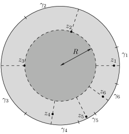
Figure 1. The zeros are placed on radii at least a distance $R$ away from the origin, that is, in the lightly shaded region.

Before focusing on the general case, we find the solutions in some specific examples.

Example 3.

Assume all arcs have the same length, $\frac{2\pi}{N}$. In this case, symmetry considerations imply that if the zeros are placed on radii that satisfy condition i), then all the zeros must be placed at the same distance $r$ away from the origin. For $r\geq R$ also condition ii) is fulfilled. Using the symmetry we may calculate

$$\delta(B)=\frac{Nr^{N-1}}{1+r^{2}+r^{4}+\cdots+r^{2(N-1)}}.$$

Example 4.

Given two arcs $\gamma_{1}$ and $\gamma_{2}$ with lengths $|\gamma_{1}|=\theta$ and $|\gamma_{2}|=2\pi-\theta$. We may assume that $\theta\leq\pi$ and that the arcs lie symmetrically about the real axis. To satisfy condition i), the zeros must be $z_{1}=r_{1}$ and $z_{2}=-r_{2}$ for $r_{1},r_{2}\in[0,1)$, and

$$B(z)=\lambda\frac{z-r_{1}}{1-r_{1}z}\frac{z+r_{2}}{1+r_{2}z}.$$

As $B(\bar{z})=\overline{B(z)}$ and $B(1)=\lambda$, we need to find $r_{1}$ and $r_{2}$ such that

$$B(e^{-i\theta/2})=B(e^{i\theta/2})=-\lambda.$$

Solving the resulting second-order equation in $e^{i\theta/2}$ yields

$$\cos\tfrac{1}{2}\theta=\frac{r_{1}-r_{2}}{1-r_{1}r_{2}}\qquad\text{or}\qquad r_{1}=\frac{r_{2}+\cos\frac{1}{2}\theta}{1+r_{2}\cos\frac{1}{2}\theta}.$$

Because $\theta\leq\pi$ we get that $r_{1}\geq r_{2}$, so by choosing $r_{2}\geq R$ the Blaschke product satisfies condition ii). The uniform separation constant will be

$$\delta(B)=\frac{r_{1}+r_{2}}{1+r_{1}r_{2}}.$$

We also remark that if $r_{2}=0$, then $r_{1}=\cos\frac{1}{2}\theta$. This is the $N=2$ version of a beautiful geometrical result by U. Daepp, Gorkin and Mortini [2].

2. Constructing interpolating Blaschke products

In this section we prove Theorem 1 by devising an iterative algorithm that solves the problem. The crucial ingredients in the algorithm are certain monotonicity relationships. To describe these we use the harmonic measure.

Recall that for a measurable set $E\subset\partial\mathbb{D}$ the harmonic measure of $E$ at a point $z\in\mathbb{D}$ is

$$\omega(z,E;\mathbb{D})=\int_{E}\frac{1-|z|^{2}}{|e^{i\theta}-z|^{2}}\,\frac{\mathrm{d}\theta}{2\pi}.$$

On $\partial\mathbb{D}$ the derivative of the argument of a Blaschke product is

$$\tfrac{\mathrm{d}}{\mathrm{d}\theta}\bigl{(}\arg B(e^{i\theta})\bigr{)}=\tfrac{\mathrm{d}}{\mathrm{d}\theta}\operatorname{Im}\bigl{(}\log B(e^{i\theta})\bigr{)}=\sum_{n=1}^{N}\frac{1-|z_{n}|^{2}}{|e^{i\theta}-z_{n}|^{2}}.$$

Therefore we consider the measure $\mu$ defined by

$$\mu(E)=\sum_{n=1}^{N}\omega(z_{n},E;\mathbb{D})=\sum_{n=1}^{N}\int_{E}\frac{1-|z_{n}|^{2}}{|e^{i\theta}-z_{n}|^{2}}\,\frac{\mathrm{d}\theta}{2\pi}.$$ (2)

With this notation our problem is to find conditions on $z_{1},\ldots,z_{N}$ such that $\mu(\gamma_{n})=1$ for each arc $\gamma_{1},\ldots,\gamma_{N}$. We first make some observations about $\mu$.

Lemma 5.

The measure $\mu$ corresponding to the zeros $z_{1},\ldots,z_{N}$ has the following properties.

1. $\mu(\partial\mathbb{D})=\sum_{n=1}^{N}\mu(\gamma_{n})=N$.

2. $\mu(\gamma_{n})\in(0,N)$.

3. $\omega(z_{n},\gamma_{n};\mathbb{D})$ is increasing as a function of $|z_{n}|$.

4. If $|z_{n}|$ is large enough, then $\omega(z_{n},\gamma_{m};\mathbb{D})$, $m\neq n$, is decreasing as a function of $|z_{n}|$.

5. $\omega(0,\gamma_{n};\mathbb{D})=\frac{|\gamma_{n}|}{2\pi}$, $\lim_{|z_{n}|\rightarrow 1}\omega(z_{n},\gamma_{n};\mathbb{D})=1$ and for $n\neq m$

   $$\lim_{|z_{n}|\rightarrow 1}\omega(z_{n},\gamma_{m};\mathbb{D})=0.$$

Proof.

All these properties are easy observations. Properties (a) and (b) follow because $\omega$ is a probability measure in the second variable. Property (e) comes from the definition of harmonic measure, while properties (c) and (d) follow from considerations about the radial derivative of

$$\frac{1-|z_{n}|^{2}}{|e^{i\theta}-z_{n}|^{2}}.$$

These considerations also give a sufficient condition for (d) to hold. Namely,

$$|z_{n}|\geq\frac{1-\sin\frac{1}{2}|\gamma_{n}|}{\cos\frac{1}{2}|\gamma_{n}|}.$$

∎

We will now describe the algorithm for constructing a sequence of Blaschke products $(B_{k})$, which converges to the Blaschke product we seek. All the Blaschke products $B_{k}$ will satisfy the extra conditions i) and ii). We denote the zeros of $B_{k}$ by $z_{k,n}$. Similarily, $\mu_{k}$ denotes the measure defined by (2) corresponding to the zeros $\{z_{k,n}\}$. To initiate the algorithm, we calculate the mid-point of each arc and call it $e^{i\theta_{n}}$, $n=1,\ldots,N$. The zeros of the initial Blaschke product, $B_{0}$, are set to be $z_{0,n}=Re^{i\theta_{n}}$ for $n=1,\ldots,N$, where $R\in[0,1)$ is chosen to be large enough in two respects. First of all, $R$ needs to be large enough for Lemma 5(d) to hold. A sufficient condition for this will be

$$R\geq\frac{1-\sin\frac{1}{2}L_{\gamma}}{\cos\frac{1}{2}L_{\gamma}},$$ (3)

where $L_{\gamma}$ is the length of the shortest arc, $L_{\gamma}=\min_{1\leq n\leq N}|\gamma_{n}|$. Furthermore, $R$ needs to be large enough to make $\delta(B_{0})>C$. See Figure 3 for an example.

The iteration proceeds in the following manner. The Blaschke product $B_{k+1}$ is constructed from $B_{k}$ by moving one of the zeros along its corresponding radius towards the boundary $\partial\mathbb{D}$. To choose which zero is moved, calculate the measures $\mu_{k}(\gamma_{n})$ for $n=1,\ldots,N$ corresponding to the Blaschke product $B_{k}$. If all these measures are $1$, we are done. If not, identify the index of the arc with the smallest measure and call this index $m$. The Blaschke product $B_{k+1}$ will have the same zeros as $B_{k}$, except $z_{m}$ which is moved along its given radius so that for $B_{k+1}$ the measure $\mu_{k+1}(\gamma_{m})=1$. See Figure 4 for an example, while Figure 2 gives the metacode for the algorithm.

  Given:

• $N$ disjoint arcs, $\gamma_{1},\ldots,\gamma_{N}$.

• The bound $C<1$ for the separation constant.

• The accuracy $\varepsilon>0$.

Algorithm:

1. Construct $B_{0}$.

   • Calculate the mid-points $e^{i\theta_{n}}$.

   • Choose $R$.

   • Set $z_{0,n}=Re^{i\theta_{n}}$.

   • Set $k=0$.

2. Calculate the measures $\mu_{k}(\gamma_{n})$ corresponding to the zeros of $B_{k}$, and the error

   $$E_{k}=\sum_{n=1}^{N}\bigl{|}1-\mu_{k}(\gamma_{n})\bigr{|}.$$

   If $E_{k}<\varepsilon$ then stop the algorithm.

3. Find the index $m$ of the arc with smallest measure. (If there are several arcs with the smallest measure, choose the index of any of them.)

4. Set $z_{k+1,n}=z_{k,n}$ for all $n\neq m$, and choose $z_{k+1,m}$ such that $\mu_{k+1}(\gamma_{m})=1$.

5. Increase $k$ by one, and return to Step 2.

 

Figure 2. Metacode for the algorithm described in Section 2.

We first remark that such an iteration is always possible. If $\mu(\gamma_{n})\neq 1$ for some $n=1,\ldots,N$, then by Lemma 5(a) and 5(b) there is at least one arc $\gamma_{m}$ such that $\mu(\gamma_{m})<1$. Using Lemma 5(c) and 5(e) we see that there is a point on the line segment between $|z_{k,m}|e^{i\varphi_{m}}$ and $e^{i\varphi_{m}}$ where $z_{k+1,m}$ can be placed in order to give $\mu_{k+1}(\gamma_{m})=1$ for $B_{k+1}$.

Next, we observe that if $\mu_{k}(\gamma_{n})\leq 1$ for some $k$, then also $\mu_{j}(\gamma_{n})\leq 1$ for all $j\geq k$, as the only way to increase the measure of an arc is to move its corresponding zero, and this will never increase the measure beyond $1$. This implies that there is at least one arc $\gamma_{l}$ for which $\mu_{k}(\gamma_{l})\geq 1$ for all $k\in\mathbb{N}$, and in consequence that there is at least one zero $z_{l}$ which is never moved. That is, at least one zero lies at the initial distance from the origin $R$ in all Blaschke products $B_{k}$, $k\in\mathbb{N}$.

Finally, we comment that the sequence $(B_{k})$ converges to a Blaschke product with the desired properties. Let $B=\lim_{k\rightarrow\infty}B_{k}$. Because the zeros are always moved outwards, we will have $\delta(B)\geq\delta(B_{0})$ such that a proper choice of $R$ will guarantee that $\delta(B)>C$. Thus, we only need to show that $\mu(\gamma_{n})=1$, $n=1,\ldots,N$, for the measure corresponding to the zeros of $B$. For each Blaschke product $B_{k}$ define the error

$$E_{k}=\sum_{n=1}^{N}\bigl{|}1-\mu_{k}(\gamma_{n})\bigr{|}.$$

Clearly, $E_{k}\geq 0$. Furthermore $E_{k+1}\leq E_{k}$ as the arcs with $\mu_{k}(\gamma_{n})>1$ will contribute to a lower error, since their measures decrease in every step. Hence $(E_{k})$ is a convergent sequence. To see that $(E_{k})$ converges to $0$ we argue that the decrease of $E_{k}$ at each step is comparable to $E_{k}$ itself. Let $\gamma_{l}$ be an arc such that $\mu_{k}(\gamma_{l})\geq 1$ for every $k\in\mathbb{N}$. Then the length of $\gamma_{l}$ is at least $c\frac{2\pi}{N}$ for some $c>0$. Furthermore, if $\gamma_{m}$ is the arc with smallest measure at some step $k$, then $\mu_{k}(\gamma_{m})\leq 1-[2(N-1)]^{-1}E_{k}$. When moving $z_{m}$, the decrease in measure from step $k$ to step $k+1$ is more or less evenly distributed outside the arc $\gamma_{m}$. This means that the decrease $\mu_{k}(\gamma_{l})-\mu_{k+1}(\gamma_{l})$ is at least $\tilde{c}[2N(N-1)]^{-1}E_{k}$, and consequently that

$$E_{k}-E_{k+1}\geq\tilde{c}[2N(N-1)]^{-1}E_{k},\quad\text{for some $\tilde{c}>0$}.$$ (4)

Thus, $E_{k}$ converges exponentially to $0$.

Example 6.

Assume that we are given arcs $\gamma_{1},\ldots,\gamma_{6}$ with lengths $\frac{\pi}{5}$, $\frac{3\pi}{5}$, $\frac{3\pi}{5}$, $\frac{3\pi}{10}$, $\frac{\pi}{10}$ and $\frac{\pi}{5}$ respectively. We want to find a Blaschke product $B$ with $\delta(B)>C=0.7$, that maps each arc onto the unit circle.

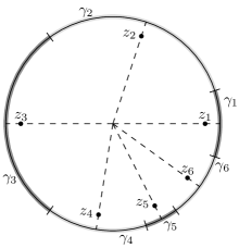
$n$ $|z_{n}|$ $\mu(\gamma_{n})$ 1 0. 8600 0. 8850 2 0. 8600 1. 1759 3 0. 8600 1. 1254 4 0. 8600 1. 1207 5 0. 8600 0. 6459 6 0. 8600 1. 0471

Figure 3. The Blaschke product $B_{0}$ in Example 6. The error is $E_{0}\approx 0.9383$.

We start by constructing $B_{0}$, and first we calculate the mid-points. We may assume that $\theta_{1}=0$. Then

$$\theta_{2}=\tfrac{2\pi}{5},\quad\theta_{3}=\pi,\quad\theta_{4}=\tfrac{29\pi}{20},\quad\theta_{5}=\tfrac{33\pi}{20}\quad\text{and}\quad\theta_{6}=\tfrac{9\pi}{5}.$$

As the shortest arc is $\gamma_{5}$ with length $\pi/10$, we need

$$R\geq\frac{1-\sin(\pi/20)}{\cos(\pi/20)}\approx 0.8541$$

to satisfy (3). Trying with $R=0.855$, we see that

$$\delta(B_{0})=\min_{k}\prod_{j\neq k}\frac{R|e^{i\theta_{j}}-e^{i\theta_{k}}|}{|1-R^{2}e^{\theta_{j}-\theta_{k}}|}\approx 0.6854.$$

As this is less than $C$, we try with a bigger $R$. A new calculation shows that $R=0.86$ gives $\delta(B_{0})\approx 0.7025>C$, so we use this $R$ as the initial radius.

Next, we start the iteration. First we calculate the $\mu$-measures of the arcs for $B_{0}$. The result is shown in Figure 3. We see here that $\gamma_{5}$ is the arc with smallest measure. Thus, to construct $B_{1}$ from $B_{0}$ we will move the zero $z_{5}$. As $\gamma_{5}$ has start-point $e^{i16\pi/10}$ and end-point $e^{i17\pi/10}$, we need to find conditions on $|z_{5}|$ such that

$$B_{1}(e^{i16\pi/10})=B_{1}(e^{i17\pi/10}),$$

which will imply that $\mu_{1}(\gamma_{5})=1$. Since we now all the other zeros of $B_{1}$, this just amounts to solving a second degree equation in $|z_{5}|$, and we find that $|z_{5}|\approx 0.9675$ is a solution. Hence, we have found $B_{1}$. See Figure 4.

$n$ $|z_{n}|$ $\mu(\gamma_{n})$ 1 0. 8600 0. 8623 2 0. 8600 1. 1526 3 0. 8600 1. 0966 4 0. 8600 0. 9739 5 0. 9675 1. 0000 6 0. 8600 0. 9146

Figure 4. The Blaschke product $B_{1}$. To construct $B_{1}$ from $B_{0}$, the zero $z_{5}$ is moved. After 1 iteration, the error is $E_{1}\approx 0.4983$.

We then continue in the same manner to construct $B_{2}$, $B_{3}$, and so on. To construct $B_{2}$ from $B_{1}$ we move the zero $z_{1}$. Figure 5 shows the Blaschke product $B_{75}$. As $E_{75}\approx 1.4\cdot 10^{-5}$ this is a quite good approximation to the true solution $B$.

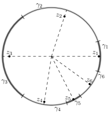
$n$ $|z_{n}|$ $\mu(\gamma_{n})$ 1 0. 9692 1. 0000 2 0. 8600 1. 0000 3 0. 8616 1. 0000 4 0. 9431 1. 0000 5 0. 9884 1. 0000 6 0. 9646 1. 0000

Figure 5. After 75 iterations, $B_{k}$ approximates the true solution quite well. The error $E_{75}$ is approximately $1.4\cdot 10^{-5}$.

3. Variations of the result

Note that there is nothing special about the mid-points of the arcs that we chose in the extra condition i). We could let each zero move along any radius that ends inside the corresponding arc. We do not even need to use radii. We only need the zeros to move along curves such that the monotonicity criteria in Lemma 5 hold. This implies one of the strengths of our proof. Because of the flexibility of the harmonic measure, it will apply even to more general domains than the unit disk. The proof runs through in any domain where we can define a measure $\mu$ that satisfies Lemma 5. Hence, we have the following.

Corollary 7.

Let $\Gamma\subset\overline{\mathbb{D}}$ be a closed Jordan curve, and let $\varphi_{1},\ldots,\varphi_{N}$ be distinct points on $\Gamma$. For every $C<C_{\Gamma}$ there is a finite Blaschke product $B$ of degree $N$ with zeros inside $\Gamma$ such that $\delta(B)>C$ and

$$\arg B(\varphi_{1})=\cdots=\arg B(\varphi_{N}).$$

The curve $\Gamma$ puts natural restrictions on how separated the zeros of the Blaschke product can be. This is reflected in the constant $C_{\Gamma}$, which will depend on the curve $\Gamma$ and the choice of curves that the zeros are moved along during the algorithm.

In [3] Gorkin and Mortini proved that given a (possibly infinite) sequence $(\lambda_{k})$ of distinct points on the unit circle, then for a sequence $(a_{k})\subset\overline{\mathbb{D}}$ there is an interpolating Blaschke product with radial limits $a_{k}$ at $\lambda_{k}$ for all $k$ if and only if $(a_{k})$ is bounded away from zero. To prove this, Gorkin and Mortini needed a little more than what is stated in Theorem 1. In their paper, they showed the following.

Theorem 8.

Let $s$ be a real number satisfying $0<s<1$. Suppose that $\varphi_{1},\ldots,\varphi_{N+1}$ are distinct points on the unit circle and let $\beta\in\partial\mathbb{D}\setminus\{1\}$. Then for every $C$ with $0<C<1$ and $m\in\mathbb{N}$ there exists a Blaschke product $B$ of degree $N$ such that

1. $B(\varphi_{j})=1$ for $j=1,\ldots,N$,

2. $B(\varphi_{N+1})=\beta$,

3. $|1-B(z)|<2^{-m-2}$ for $|z|\leq s$,

4. $|1-B(r\varphi_{j})|<2^{-m}$ for $j=1,\ldots,N$ and $0<r\leq 1$,

5. $\delta(B)\geq C$.

In addition, the following also hold:

1. Let $E\subset\mathbb{D}$. If the pseudo-hyperbolic distance between any two distinct points in $E$ is at least $\rho$, then the zero of $B$ closest to $\varphi_{N+1}$, can be chosen to be at pseudo-hyperbolic distance at least $\rho/3$ to the points of $E$.

2. It is possible to choose the zeros $z_{1},\ldots,z_{N}$ of $B$ so that

   $$\tfrac{1-|z_{j}|}{|z_{j}-\varphi_{k}|}\leq 2^{-m}\quad\text{for $j=1,\ldots,N-1$ and $k=1,\ldots,N+1$}$$

   and such that $z_{N}$ is close to $\varphi_{N+1}$.

We stated Theorem 1 in its simple form in order to emphasize the ideas behind the proof. However, with some minor modifications of our algorithm and some careful bookkeeping we can indeed prove Theorem 8 as well.

Proof of Theorem 8.

By identifying the points $\varphi_{1},\ldots,\varphi_{N}$ with the end-points of the arcs $\gamma_{1},\ldots,\gamma_{N}$ and choosing a proper rotation $\lambda$ we have already proved (a) and (e). To satisfy (b) we need to add one degree of freedom to our construction. We no longer demand that the zero $z_{N}$ be placed on the radius through the mid-point of the arc $\gamma_{N}$. Instead we demand that this zero be placed in the sector between $\varphi_{N}$ and $\varphi_{1}$. This can be done using a 2-step algorithm. First we choose some admissible radius at angle $\theta$ for the zero $z_{N}$ to move along, and run the usual algorithm to construct a Blaschke product $B_{\theta}$. If we find that

$$\arg B_{\theta}(\varphi_{N+1})<\arg\beta$$

we need to choose a smaller $\theta$ and try again. Conversely, if $\arg B_{\theta}(\varphi_{N+1})>\arg\beta$ we need to choose a bigger $\theta$. For the different angles we need to keep $R$ fixed and large enough, where what is large enough may also depend on $\beta$. For a properly chosen sequence of angles this process converges to a Blaschke product which satisfies (b) in addition to (a) and (e).

Properties (c) and (d) will hold if we choose the zeros close enough to the boundary. In this case the Blaschke product is essentially constant and close to 1 outside the darkly shaded regions in Figure 6, and the disk $\{z\colon|z|<s\}$ and the rays $\{z=r\varphi_{j}\colon j=1,\ldots,N,0<r\leq 1\}$ do not meet these regions.

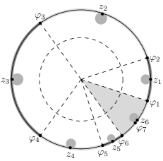
Figure 6. The Blaschke product is essentially constant and close to 1 outside the darkly shaded region. The disk and the rays indicated with dashed lines do not meet these regions. The zero $z_{N}$ (here $N=6$) is placed somewhere inside the lightly shaded sector.

The possible positions for the zero $z_{N}$ in order to fulfill (b) will lie on a curve, parameterized by the initial radius $R$, ending in the point $\varphi_{N+1}$. Since any point close to $\varphi_{N+1}$ lying on the curve will yield a solution, we see that i) and the last part of ii) holds. The first part of ii) says that the zeros $z_{1},\ldots,z_{N-1}$ can be chosen to be much closer to the boundary than to the points $\varphi_{1},\ldots,\varphi_{N+1}$, which holds true by construction. ∎

Properties (a) and (b) in Theorem 8 give an easy way to construct solutions to general finite interpolation problems on the circle of the form (1). Namely, construct Blaschke products $b_{1},\ldots,b_{N}$ which each satisfy

$$b_{k}(\varphi_{k})=\psi_{k}\qquad\text{and}\qquad b_{k}(\varphi_{j})=1\quad\text{for $j\neq k$}$$

using Theorem 8. Then $B=\prod_{k=1}^{N}b_{k}$ satisfies

$$B(\varphi_{n})=\psi_{n},\qquad n=1,\ldots,N.$$

If we are a bit careful with the placing of the zeros of $B$, we can also make sure that this Blaschke product has arbitrarily big separation. However, this Blaschke product may have degree as high as $N(N-1)$, which is far away from the optimal $N-1$ in Theorem 2. It seems plausible that it should be possible to construct an algorithm similar to the one we have discussed here, albeit more complicated, which can solve the general finite interpolation problem on the circle with a Blaschke product of degree comparable to $N$.

References

- [1] Charles R. Collins and Kenneth Stephenson, A circle packing algorithm, Comput. Geom. 25 (2003), no. 3, 233–256.
- [2] Ulrich Daepp, Pamela Gorkin, and Raymond Mortini, Ellipses and finite Blaschke products, Amer. Math. Monthly 109 (2002), no. 9, 785–795.
- [3] Pamela Gorkin and Raymond Mortini, Radial limits of interpolating Blaschke products, Math. Ann. 331 (2005), 417–444.
- [4] William B. Jones and Stefan Ruscheweyh, Blaschke product interpolation and its application to the design of digital filters, Constr. Approx. 3 (1987), 405–409.
- [5] Gunter Semmler and Elias Wegert, Boundary interpolation with Blaschke products, Preprint.