On the validations of the
Asymptotic Matching Conjectures

Abstract

In this paper we review the asymptotic matching conjectures for $r$-regular bipartite graphs, and their connections in estimating the monomer-dimer entropies in $d$-dimensional integer lattice and Bethe lattices. We prove new rigorous upper and lower bounds for the monomer-dimer entropies, which support these conjectures. We describe a general construction of infinite families of $r$-regular tori graphs and give algorithms for computing the monomer-dimer entropy of density $p$, for any $p\in[0,1]$, for these graphs. Finally we use tori graphs to test the asymptotic matching conjectures for certain infinite $r$-regular bipartite graphs.
2000 Mathematics Subject Classification: 05A15, 05A16, 05C70, 05C80, 82B20
Keywords and phrases: Matching and asymptotic growth of average matchings for $r$-regular bipartite graphs, monomer-dimer partitions and entropies.

1 Introduction

The monomer-dimer covers of infinite graphs $G$, and in particular of the infinite graph induced by the lattice $\mathbb{Z}^{d}$, is one of the widely used models in statistical physics. See for example [1, 2, 4, 5, 6, 12, 14, 15, 16, 17, 19, 20, 21, 23, 24, 25, 26, 28, 30].

Let $G=(V,E)$ be an undirected graph with vertices $V$ and edges $E$. $G$ can be a finite or infinite graph. A dimer is a domino occupying an edge $e=(u,v)\in E$. It can be viewed as two neighboring atoms occupying the vertices $u,v\in V$ and forging a bond between themselves. A monomer is an atom occupying a vertex $w\in V$, which does not form a bond with any other vertex in $V$. A monomer-dimer cover of $G$ is a subset $E^{\prime}$ of $E$ such that any two distinct edges $e,f\in E^{\prime}$ do not have a common vertex. Thus $E^{\prime}$ describes all dimers in the corresponding monomer-dimer cover of $G$. All vertices $V^{\prime}\subset V$, which are not on any edge $e\in E^{\prime}$, are the monomers of the monomer-dimer cover represented by $E^{\prime}$. $E^{\prime}$ is referred to here as a matching. $E^{\prime}$ is called a perfect matching if $V^{\prime}=\emptyset$, i.e. all the vertices of $G$ are covered by the dimers.

Consider first a finite graph $G=(V,E)$. Then $E^{\prime}$ is called an $l$-matching if $\#E^{\prime}=l$. Note that $2l\leq\#V$. Let $\phi(l,G)\geq 0$ be the number of $l$-matchings in $G$ for any $l\in\mathbb{Z}_{+}$. (Note that $\phi(0,G)=1$ and $\phi(l,G)=0$ if there are no $l$-matchings in $G$. Assume also that $\phi(l,G)=0$ for a non-integer $l\geq 0$.) Then the monomer-dimer entropy of density $p$ of $G$ is defined as

$$h_{G}(p)=\frac{\log\max(\phi(\lfloor\frac{p\cdot\#V}{2}\rfloor,G),1)}{\#V}\textrm{ for any }p\in[0,1].$$

Let $\psi(x,G):=\sum_{l=0}^{\infty}\phi(l,G)x^{l}$ denote the matching generating polynomial of $G$. The pressure of $G$ is defined as

$$P_{G}(t):=\frac{\log\psi(e^{2t},G)}{\#V}.$$

For an infinite graph $G$ the monomer-dimer entropy of density $p$ and the pressure $P_{G}(t)$ are defined by taking appropriate $\limsup$ on the finite sequences of graphs converging to $G$. (See for details §2.)

We now consider the classical case in statistical physics: the lattice $\mathbb{Z}^{d}$, consisting of all $d$-dimensional vectors $\mathbf{i}=(i_{1},\ldots,i_{d})$ with integer coordinates. (As usual we denote by $\mathbb{Z},\mathbb{Z}_{+},\mathbb{N}$ the set of integer, the set of nonnegative integers and the set of positive integers.) Let $\mathbf{e}_{k}=(\delta_{k1},\ldots,\delta_{kd})$ be the unit vector in the direction of the coordinate $x_{k}$ for $k=1,\ldots,d$. Then $G(\mathbb{Z}^{d})=(V=\mathbb{Z}^{d},E)$, where $(\mathbf{i},\mathbf{j})\in E\iff\mathbf{j}-\mathbf{i}=\pm\mathbf{e}_{k}$ for some $k\in[1,d]$. Note that $G(\mathbb{Z}^{d})$ is an infinite $2d$ regular graph.

Let $h_{d}(p):=h_{G(\mathbb{Z}^{d})}(p)$ for any $p\in[0,1]$ and $h_{d}:=\sup_{p\in[0,1]}h_{d}(p)$. ($h_{d}$ and $\tilde{h}_{d}:=h_{d}(1)$ are called the $d$-monomer-dimer entropy and the $d$-dimer entropy respectively [12].) For $d=1$ it is known that [12, §4]:

$$h_{1}(p)=\left(1-\frac{p}{2}\right)\log\left(1-\frac{p}{2}\right)-\frac{p}{2}\log\frac{p}{2}-(1-p)\log(1-p),\quad p\in[0,1].$$ (1.1)

The value of planar dimer entropy $h_{2}(1)$ was computed in [5] and [21]

$$h_{2}(1)={1\over\pi}\sum_{q=0}^{\infty}{(-1)^{q}\over(2q+1)^{2}}=0.29156090\ldots$$

The exact values of $h_{2}(p)$ for $p\in(0,1)$ and $h_{d}(p)$ for $d\geq 3,p\in(0,1]$ are unknown. According to Jerrum [24], the computation of the matching generating polynomials of finite planar graphs in general is computationally intractable. (This fact does not rule out the possibility that $h_{d}(p)$ are computationally tractable for $d\geq 2$, however for $d\geq 3$ it seems that $h_{3}(1)$ and $h_{3}$ are hard to compute with high precision.)

The properties of the entropy $h_{d}(p)$ for any $p\in[0,1]$ was studied by Hammersley and his collaborators in [15, 16, 17, 19]. It was shown in [12] that $h_{d}(p)$ can be obtained from the limits of certain tori graphs, which are bipartite and $2d$ regular. Using the proof of Tverberg’s permanent conjecture, proved by the first name author [8], the following lower bound was shown in [12]

$$h_{d}(p)\geq fh_{d}(p):={\textstyle\frac{1}{2}}(-p\log p-2(1-p)\log(1-p)+p\log 2d-p)$$ (1.2)

for any $p\in[0,1]$.

Tverberg’s permanent conjecture states that the minimum of the sum of all $l\times l$ permanental minors of $n\times n$ doubly stochastic matrices is achieved only at the flat matrix $J_{n}=(\frac{1}{n})$. It is a generalization of the van der Waerden permanent conjecture for doubly stochastic matrices, which is the case $l=n$. In [32] Schrijver gave a lower bound on the number of perfect matchings for $r$-regular bipartite graphs. It is an improvement of the lower bound implied by the van der Waerden permanent conjecture. Furthermore, this lower bound is asymptotically sharp. Equivalently, one can think that Schrijver’s lower bound gives asymptotically the number of perfect matchings in large random $r$-regular bipartite graph.

In [11] we stated a Lower Matching Conjecture, referred here as LMC, for any $l$-matchings of $r$-regular bipartite graph. For $2l=\#V$ this conjecture is asymptotically equivalent to Schrijver lower bound for perfect matchings. This lower bound can be viewed asymptotically as the number of $l$-matchings in a large random $r$-regular bipartite graph. The LMC implies the Lower Asymptotic Matching Conjecture stated in §2, referred here as LAMC, yields the following conjecture.

$$h_{d}(p)\geq gh_{2d}(p),\texttt{ for any }p\in(0,1]\texttt{ and }d\geq 2,$$ (1.3)

where

$$gh_{r}(p):=\frac{1}{2}\big{(}p\log r-p\log p-2(1-p)\log(1-p)+(r-p)\log(1-\frac{p}{r})\big{)},$$ (1.4)

for any integer $r\geq 2$. Note that $h_{1}(p)=gh_{2}(p)$. In a recent paper [10] the LAMC was proven for the sequence of densities $p=\frac{r}{r+s},s=0,1,\ldots$, for any given $r\geq 2$. Hence (1.3) holds for $p=\frac{2d}{2d+s},s=0,1,\ldots$. In particular $h_{d}(1)\geq gh_{2d}(1)$ for any $d\in\mathbb{N}$. The inequality $h_{3}(1)\geq 0.440075$ is the best known lower bound. A recent massive computation performed by the third named author in [26] gives the best known upper bound $h_{3}(1)\leq 0.457547$.

The conjectured lower bound (1.3) yields a lower bound for the $d$-monomer-dimer entropy $h_{d}$. In particular, the conjectured lower bound (1.3) yields $h_{3}\geq 0.784992989$. The validity of (1.3) for $d=3,p=\frac{6}{6+3}=\frac{2}{3}$ implies the best lower bound known $h_{3}\geq h_{3}(\frac{2}{3})\geq.7845241927$. In this paper we give new lower bounds on $h_{d}(p)$ which yield the inequality $h_{3}\geq h_{3}(0.6814)\geq.7849602275$. The numerical computations in [12] yield the best known upper bound $h_{3}\leq 0.7862023450$.

In [11] we stated an Upper Matching Conjecture, referred here as UMC. Namely, let $K_{r,r}$ be a complete bipartite graph on $2r$ vertices, where the degree of each vertex is $r$. Denote by $qK_{r,r}$ be the graph consisting of $q$ copies of $K_{r,r}$. Then the UMC claims that any $r$-regular bipartite graph $G$ on $2qr$ vertices satisfies $\phi(l,G)\leq\phi(l,qK_{r,r})$ for $l=0,\ldots,qr$. We also have a corresponding Upper Asymptotic Matching Conjecture, referred here as UAMC, which is slightly more technical to state. (See §6.) For $r=2$ we proved these conjectures in [11].

The main purpose of this paper is to give theoretical and numerical evidences on the LAMC and UAMC and their applications to the estimates of the monomer-dimer $p$-densities for $\mathbb{Z}^{d}$ and for the Bethe lattices, i.e. $d$-regular infinite trees. We believe that the computational and theoretical setting discussed in this paper are of interest by itself and to researchers in asymptotic combinatorics, which is widely used in statistical physics.

We now outline briefly the main setting of our computations for the verification of the two asymptotic conjectures. It is well known that the asymptotic growth of many configurations in statistical physics are given in terms of the spectral radius of the transfer matrix. See for example [12]. In this paper we construct infinite families $G_{n}=(V_{n},E_{n}),n\in\mathbb{N}$ of $r$-regular bipartite graphs, which are coded by a specific incidence matrix $A\in\{0,1\}^{N\times N}$. This sequence of graphs converges to an infinite $r$-regular graph $G$. Using programs based on software developed by the third named author one obtains the transfer matrix $B(t)\in\mathbb{R}^{2^{N}\times 2^{N}}$, corresponding to the matching generating polynomial with the value $x=e^{2t}$. Since the infinite tori graphs corresponds to a subshifts of finite type, abbreviated here as SOFT, one can compute the pressure function $P(t)$ in terms of the spectral radius $\rho(B(t))$. This is well known to the experts, and we bring the proofs of these formulas in the paper for completeness, using the general techniques in [13]. (The properties of the pressure function $P(t),t\in\mathbb{R}$, for multi-dimensional SOFT, as for example the monomer-dimer models in $\mathbb{Z}^{d},d>1$, are studied in detail in [13].) Then the monomer-dimer $p$-density $h_{G}(p)$ is computed by using $\rho(B(t))$ and its derivative. (In this setting $p=p(t)$.) We then compare $h_{G}(p(t))$ to the upper and lower bound given by the lower and upper asymptotic conjecture.

We now briefly survey the contents of our paper. In §2 we discuss the monomer-dimer entropy $h_{\{G_{n}\}}(p)$ of density $p$ and the pressure function $P_{\{G_{n}\}}(t)$ for a sequence of finite graphs $\{G_{n}=(V_{n},E_{n})\}$ of bounded degrees such that $\#V_{n}\to\infty$. We define the function $\mathop{\mathrm{low}}\nolimits_{r}(p),p\in[0,1]$ which gives the sharp inequality $h_{\{G_{n}\}}(p)\geq\mathop{\mathrm{low}}\nolimits_{r}(p)$ for any sequence of bipartite $r$-regular graphs and any $p\in[0,1]$. We state the LAMC, which is equivalent to the equality $\mathop{\mathrm{low}}\nolimits_{r}=gh_{r}$. Furthermore if the sequence $\{G_{n}\}$ is a sequence of random $r$-regular bipartite graphs we conjecture that $h_{\{G_{n}\}}(p)=gh_{r}(p)$ almost surely [11]. In §3 we use the recent verification of the LAMC for $p=\frac{r}{r+s},s=0,1,\ldots$ for any $r\geq 2$ to derive tight lower bounds on for $\mathop{\mathrm{low}}\nolimits_{r}$. In §4 we discuss the applications of our results to Bethe lattices, i.e. infinite dimensional $r$-regular trees. In §5 we discuss the sequence of tori graphs, which are considered in [12] and [13] to compute $h_{2},h_{3}$ and $h_{2}(p)$. We prove the thermodynamics formalisms for such graphs which gives the monomer-dimer entropy of density $p$ in terms of the pressure. In §6 we describe a fairly general construction of sequences of regular graphs, which includes the sequence of tori graphs. In §7 we describe the upper matching conjecture and its asymptotic version, called the upper asymptotic matching conjecture. We give upper bounds for $h_{\{G_{n}\}}(p)$ for any sequence of bipartite $r$-regular graphs and show that in some regions these bounds are relatively close to the UAMC. In §8 we describe our computational results, which support the conjectures stated in this paper. In §9 we identify an infinite graph with the maximal pressure among other infinite graphs in certain families of sequences described in §6.

2 Entropies, Pressure and LAMC

We will now define a limiting monomer-dimer density for a sequnce of bounded degree graphs.

      Definition 2.1

Let $\{G_{n}\},G_{n}=(V_{n},E_{n}),n\in\mathbb{N}$ be a sequence of finite graphs, where multi edges are allowed, such that $\#V_{n}\to\infty$ and the degree of each vertex in $G_{n}$ is bounded by $d$ for $n\in N$. For $p\in[0,1]$ we define $h_{\{G_{n}\}}(p)$, the monomer-dimer entropy of density $p$, as follows:

$$h_{\{G_{n}\}}(p)=\limsup_{n\to\infty}\frac{\log\phi(l_{n},G_{n})}{\#V_{n}},$$ (2.1)

$$\texttt{ over all sequences }l_{n}\in\mathbb{Z}_{+}\texttt{ satisfying }\lim_{n\to\infty}\frac{2l_{n}}{\#V_{n}}=p\in[0,1].$$ (2.2)

$h_{\{G_{n}\}}(1)$ and $h_{\{G_{n}\}}:=\sup_{p\in[0,1]}h_{\{G_{n}\}}(p)$ are called the dimer entropy of $\{G_{n}\}$, and the monomer-dimer entropy of $\{G_{n}\}$ respectively. For $t\in\mathbb{R}$ the pressure of $\{G_{n}\}$ is defined as

$$P_{\{G_{n}\}}(t):=\limsup_{n\to\infty}\frac{\log\psi(e^{2t},G_{n})}{\#V_{n}}.$$ (2.3)

Let $G=(V,E)$ be an infinite graph, where multi edges are allowed. Assume that the maximal degree of vertices in $G$ is $d<\infty$. A sequence of graphs $\{G_{n}\},G_{n}=(V_{n},E_{n}),\;V_{n}\subset V,n=1,2,\ldots,V_{n}$, where multi edges are allowed, converges to $G$ if the following conditions hold:

1. $V_{1}\subset V_{2}\subset\ldots$ are finite subsets of $V$ satisfying the condition $V=\cup_{n=1}^{\infty}V_{n}=V$.

2. Each $G_{n}$ contains the induced subgraph $G(V_{n}):=(V_{n},E(V_{n}))$ of $G$ on the set of vertices $V_{n}$, and the degree of each vertex in $G_{n}$ is at most $d$.

3. Let $v\in V_{n}$ and assume that all neighbors of $v$ in $V$ are in $V_{n}$. Then $E$ and $E_{n}$ have the same set of edges that contain $v$.

Then $h_{G}(p):=h_{\{G_{n}\}}(p),\;h_{G}:=h_{\{G_{n}\}},\;P_{G}(t):=P_{\{G_{n}\}}(t)$.

The above definition of entropy and pressure of an infinite graph $G$ depends on the specific choice of the convergent sequence $\{G_{n}\}$ to the infinite graph $G$. For $G(\mathbb{Z}^{d})$ one has a whole class of the sequences $\{G_{n}\}$, for which the resulting $h_{\{G_{n}\}}(p),P_{\{G_{n}\}}(t)$ is independent of the choice of the convergent sequence $\{G_{n}\}$ [15, 16, 17, 19, 13]. In this case we denote by $h_{d}(p),P_{d}(t)$ the corresponding quantities. For other infinite graphs $G$ discussed in this paper we choose a convenient convergent sequence $\{G_{n}\}$, and we do not discuss the corresponding class of sequences which yield the same entropy and pressure.

The properties of the entropy $h_{d}(p)$ for any $p\in[0,1]$ was studied by Hammersley and his collaborators in [15, 16, 17, 19]. Let us mention two properties that are of interest in this context. For any $m\in\mathbb{N}$ let $\langle m\rangle:=\{1,\ldots,m\}=[1,m]\cap\mathbb{Z}$ be the set of integers between $1$ and $m$. For any $\mathbf{m}=(m_{1},\ldots,m_{d})\in\mathbb{N}^{d}$ let $\langle\mathbf{m}\rangle:=\langle m_{1}\rangle\times\ldots\times\langle m_{d}\rangle\subset\mathbb{N}^{d}$ is the set of points in the lattice $\mathbb{Z}^{d}$ located in the box $[1,m_{1}]\times\ldots\times[1,m_{d}]$ in $\mathbb{R}^{d}$. Denote by $\mathrm{vol}(\mathbf{m}):=\prod_{i=1}^{d}m_{i}$ the volume of the box $\langle\mathbf{m}\rangle$. Let $G(\mathbf{m}):=(\langle\mathbf{m}\rangle,E(\mathbf{m}))$ be the subgraph of $G(\mathbb{Z}^{d})$ induced by $\langle\mathbf{m}\rangle$, i.e. $(\mathbf{i},\mathbf{j})\in E(\mathbf{m})\iff\mathbf{i},\mathbf{j}\in\langle\mathbf{m}\rangle$ and $\mathbf{i}-\mathbf{j}=\pm\mathbf{e}_{k}$ for some $k\in\langle d\rangle$. Let $\mathbf{m}_{n}:=(m_{1,n},\ldots,m_{d,n}),n\in\mathbb{N}$ be a sequence of lattice points in $\mathbb{N}^{d}$, such that $\mathbf{m}_{n}\to\infty\iff m_{k,n}\to\infty$ as $n\to\infty$ for each $k=1,\ldots,d$. Then for any sequence $l_{n}\in[0,\frac{\mathrm{vol}(\mathbf{m}_{n})}{2}]\cap\mathbb{N}$ the following conditions hold:

$$\lim_{n\to\infty}\frac{\log\phi(l_{n},G(\mathbf{m}_{n}))}{\mathrm{vol}(\mathbf{m}_{n})}=h_{d}(p)\texttt{ if }\mathbf{m}_{n}\to\infty\texttt{ and }\lim_{n\to\infty}\frac{2l_{n}}{\mathrm{vol}(\mathbf{m}_{n})}=p\in[0,1].$$ (2.4)

The above characterization yields that $h_{d}(p)$ is a concave continuous function on $[0,1]$, see [15].

Let $T(\mathbf{m}):=(\langle\mathbf{m}\rangle,\tilde{E}(\mathbf{m}))$ be the torus on $\langle\mathbf{m}\rangle$. Thus two vertices $\mathbf{i},\mathbf{j}\in\langle\mathbf{m}\rangle$ in $T(\mathbf{m})$ are neighbors if $(\mathbf{i},\mathbf{j})\in E(\mathbf{m})$, or for any $m_{k}>2$ the vertices $(i_{1},\ldots,i_{k-1},1,i_{k+1},\ldots,i_{d})$ and $(i_{1},\ldots,i_{k-1},m_{k},i_{k+1},\ldots,i_{d})$ are adjacent for any $k\in\langle d\rangle$ and $(i_{1},\ldots,i_{k-1},i_{k+1},\ldots,i_{d})\in\mathbb{N}^{d-1}$. Clearly $\phi(l,T(\mathbf{m}))\geq\phi(l,G(\mathbf{m}))$ for any $l\in\mathbb{Z}_{+}$. It was shown in [12] that the condition (2.4) can be replaced by the corresponding condition on the torus:

$$\lim_{n\to\infty}\frac{\log\phi(l_{n},T(\mathbf{m}_{n}))}{\mathrm{vol}(\mathbf{m}_{n})}=h_{d}(p)\texttt{ if }\mathbf{m}_{n}\to\infty\texttt{ and }\lim_{n\to\infty}\frac{2l_{n}}{\mathrm{vol}(\mathbf{m}_{n})}=p\in[0,1].$$ (2.5)

(It is assumed that $l_{n}\in[0,\frac{\mathrm{vol}(\mathbf{m}_{n})}{2}]\cap\mathbb{N}$.) More general, one can show that $h_{d}(p)=h_{G(\mathbb{Z}^{d})}(p)$.

There are several advantages of considering $T(\mathbf{m})$ over $G(\mathbf{m})$. Assume that $m_{k}>2$ for $k=1,\ldots,d$. First, the graph $T(\mathbf{m})$ is a $2d$-regular graph. Second, the automorphism group of $T(\mathbf{m})$ is quite big, which can be very well exploited, using the general method of [26]. See also[27], and [12, 13] for the computations of $h_{d},\tilde{h}_{d}$ and $h_{d}(p)$ respectively.

The fact that $T(2\mathbf{m})$ is $2d$-regular bipartite graph was exploited in [12] to show (1.2). This lower bound is obtained by noting that if $G=(V,E)$ is an $r$-regular bipartite graph then $\phi(l,G)\geq f_{r}(l,\#V)$, where the function $f_{r}(l,2n):=\binom{n}{l}^{2}l!\,\left(\frac{r}{n}\right)^{l}$ is determined from the proof of Tverberg’s permanent conjecture [8].

The LMC stated in [11] claims that $\phi(l,G)\geq g_{r}(l,\#V)\;(\geq f_{r}(l,\#V))$ for any $r$-regular bipartite graph, where.

$$g_{r}(l,2n)={n\choose l}^{2}(\frac{nr-l}{nr})^{rn-l}(\frac{lr}{n})^{l}.$$ (2.6)

For $2l=\#V$ (2.6) is Schrijver’s lower bound for perfect matchings in $r$-regular bipartite graphs on $2n$ vertices. The LAMC, which yields(1.3), can be stated as follows:

      Conjecture 2.2

( The Lower Asymptotic Matching Conjecture.) Let $\mathcal{G}(2n,r)$ be the set of $r$-regular bipartite graphs on $2n$ vertices, possibly with multi edges. For each $l\in[0,n]\cap\mathbb{Z}$ let $\mu(l,2n,r):=\min_{G\in\mathcal{G}(2n,r)}\phi(l,G)$. For $p\in[0,1]$ let $\mathop{\mathrm{low}}\nolimits_{r}(p)$ be the infimum $\liminf_{n\to\infty}\frac{\log\mu(l_{k},2n_{k},r)}{2n_{k}}$ over all sequences $0\leq l_{k}\leq n_{k},k\in\mathbb{N}$ such that $lim_{k\to\infty}\frac{2l_{k}}{2n_{k}}=p$. Then

$$\mathop{\mathrm{low}}\nolimits_{r}(p)=gh_{r}(p).$$ (2.7)

The results in [11] show that for a given $p\in[0,1]$ and $r\geq 2$, the above conjecture is equivalent to the statement that the number of $l$-matching in a random bipartite $r$-regular graph will behave asymptotically as in Conjecture 2.2. In particular, the random graphs minimize, in the asymptotical sense, the number of $l$-matchings in $r$-regular bipartite graphs.

It is shown in [11] that the LMC and LAMC hold for $r=2$. Furthermore, the cycle $C_{2n}$ on $2n$ vertices satisfies the inequality $\phi(l,C_{2n})\leq\phi(l,G)$ for any $G\in\mathcal{G}(2n,2)$. Hence

$$\lim_{k\to\infty}\frac{\log\phi(l_{k},C_{2n_{k}})}{2n_{k}}=gh_{2}(p)=h_{1}(p)$$

for any sequence $0\leq l_{k}\leq n_{k},k\in\mathbb{N}$ satisfying the assumptions of Conjecture 2.2.

In a recent paper [10, Theorem 5.6] the following results were proven:

      Theorem 2.3

The Lower Asymptotic Matching Conjecture holds for the following corresponding sequence of densities $p=\frac{r}{r+s},s=0,1,\ldots$, for any given $r$. In particular (1.3) holds for $p=\frac{2d}{2d+s},s=0,1,\ldots$.

This can be extended to give a bound for all $p$ in the following way.

      Definition 2.4

For $2\leq r\in N$ let $ghl_{r}(p),p\in[0,1]$ be the following function.

• $ghl_{r}(\frac{r}{r+s})=gh_{r}(\frac{r}{r+s})$ for $s=0,1,\ldots$.

• $ghl_{r}(p)$ is linear on the interval $[\frac{r}{r+s+1},\frac{r}{r+s}]$ for $s=0,1,\ldots$.

• $ghl_{r}(0)=0$.

The concavity of $h_{d}(p)$ and Theorem 2.3 yields:

$$h_{d}(p)\geq ghl_{2d}(p),\textrm{ for all }p\in[0,1]\textrm{ and }d=2,3,\ldots.$$ (2.8)

In the next section we improve substantially these lower bounds.

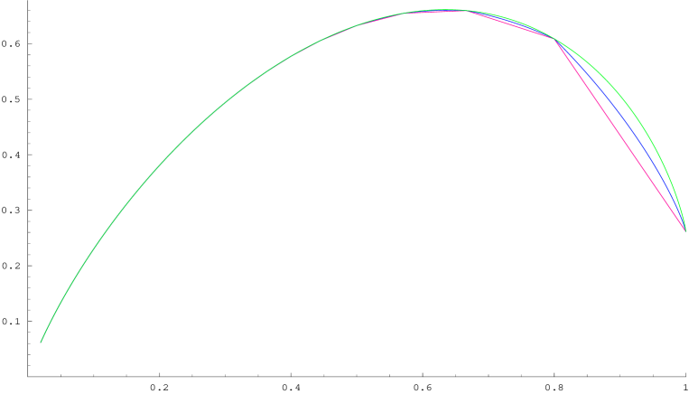
Figure 1: $ghl_{4}$-red, $\mathop{\mathrm{low}}\nolimits_{4,1}$-blue, $gh_{4}$-green, color online

In [10, Figure 1] are plotted the graph of $gh_{4}(p)$, the graph corresponding to UAMC and the 19 values of the $h_{2}(p)$ computed by Baxter [1]. (Baxter’s computations are based on sophisticated heuristical arguments. His computations were recently verified by rigorous mathematical methods in [13].) It turns out that Baxter’s values are very close to the values of $gh_{4}(p)$.

In Figure 1 we show the graphs of $ghl_{r}(p)$, $\mathop{\mathrm{low}}\nolimits_{r,1}(p)$, a lower bound for $\mathop{\mathrm{low}}\nolimits_{r}(p)$ given in the next section, and $gh_{r}(p)$ for $r=4$. Note that the differences of the three graphs are relatively large on the first interval from the right $[\frac{r}{r+1},1]$, slightly less on the second interval from the right $[\frac{r}{r+2},\frac{r}{r+1}]$, and ignorable from the fourth interval to the right $[\frac{r}{r+3},\frac{r}{r+2}]$. We notice that the differences between the functions $ghl_{r}(p),\mathop{\mathrm{low}}\nolimits_{r,1}(p),gh_{r}(p)$ decrease as $r$ increases. (This observation applies also for the values $r=3,6$ which are not plotted here.)

3 Lower bounds for $\mathop{\mathrm{low}}\nolimits_{r}(p)$

In this section we give a lower bound for the function $\mathop{\mathrm{low}}\nolimits_{r}(p)$, which is defined in Conjecture 2.2.

      Theorem 3.1

The function $\mathop{\mathrm{low}}\nolimits_{r}(p)+\frac{1}{2}(p\log p+(1-p)\log(1-p))$ is concave.

Proof. Let $G\in\mathcal{G}(2n,r)$. Consider the polynomial $\theta(x):=(-x)^{n}\psi(-\frac{1}{x},G)$. Since $\phi(l,G)>0$ for $l=0,\ldots,n$ it follows that $\theta(x)$ has $n$ complex nonzero roots. It is well known [20] that $\theta(x)$ has only positive roots. The Newton inequalities, see e.g [29], yield

$$\frac{\phi(l-1,G)}{{n\choose l-1}}\frac{\phi(l+1,G)}{{n\choose l+1}}\leq\big{(}\frac{\phi(l,G)}{{n\choose l}}\big{)}^{2},l=1,\ldots,n-1.$$ (3.1)

Let $G_{l,2n,r}\in\mathcal{G}(2n,r)$ be an $r$-regular graph for which the equality $\mu(l,2n,r)=\phi(l,G_{l,2n,r})$ holds. (3.1) and the minimal characterizations of $\mu(k,2n,r),r=0,\ldots,n$ yields

$$\frac{\mu(l-1,2n,r)}{{n\choose l-1}}\frac{\mu(l+1,2n,r)}{{n\choose l+1}}\leq\big{(}\frac{\mu(l,2n,r))}{{n\choose l}}\big{)}^{2},l=1,\ldots,n-1.$$ (3.2)

This is equivalent to the statement that the sequence

$$a_{l,2n,r}:=\log\frac{\phi(l,G)}{{n\choose l}}\geq 0,\quad l=0,\ldots,n$$

is a concave sequence. Let $\alpha(x,2n,r)$ be a piecewise linear function on $[0,1]$ defined as follows:

• $\alpha(\frac{l}{n},2n,r)=\frac{a_{l,2n,r}}{2n},\quad l=0,\ldots,n$.

• $\alpha(\frac{l}{n},2n,r)$ is linear function on the interval $[\frac{l}{n},\frac{l+1}{n}]$ for $l=0,\ldots,n-1$.

The concavity of the sequence $a_{l,2n,r},l=0,\ldots,n$ is equivalent to the concavity of $\alpha(x,2n,r)$. Let $\{n_{k}\}_{k=1}^{\infty}$ be an increasing sequence of positive integers. Let $l_{k}\in[0,n_{k}]\cap\mathbb{Z},k\in\mathbb{N}$ be a sequence satisfying $\lim_{k\to\infty}\frac{l_{k}}{n_{k}}=p\in[0,1]$. Use Stirling’s formula to deduce that

$$\lim_{k\to\infty}\frac{\log{n_{k}\choose l_{k}}}{2n_{k}}=-\frac{1}{2}\big{(}p\log p+(1-p)\log(1-p)\big{)}.$$ (3.3)

It is straightforward to show that

$$\liminf_{n\to\infty}\alpha(x,2n,r)=\mathop{\mathrm{low}}\nolimits_{r}(x)+\frac{1}{2}\big{(}p\log p+(1-p)\log(1-p)\big{)}.$$ (3.4)

Since each $\alpha(\cdot,2n,r)$ is concave it follows that $\mathop{\mathrm{low}}\nolimits_{r}(p)+\frac{1}{2}\big{(}p\log p+(1-p)\log(1-p)\big{)}$ is concave.

$\Box$

The arguments of the proof of the above Theorem combined with the definition of $h_{d}(p)=h_{G(\mathbb{Z}^{d})}(p)$, implies a stronger concavity result than given in [15].

      Corollary 3.2

Let $h_{d}(p),p\in[0,1]$ be the monomer-dimer entropy of density $p$ for the graph $G(\mathbb{Z}^{d})$. Then $h_{d}(p)+\frac{1}{2}\big{(}p\log p+(1-p)\log(1-p)\big{)}$ is concave.

Theorems 2.3 and 3.1 yields:

      Corollary 3.3

Let $\mathop{\mathrm{low}}\nolimits_{r,1}(p),p\in[0,1]$ be defined as follows.

• $\mathop{\mathrm{low}}\nolimits_{r,1}(\frac{r}{r+s})=gh_{r}(\frac{r}{r+s})$ for $s=0,1,\ldots$.

• $\mathop{\mathrm{low}}\nolimits_{r,1}(p)+\frac{1}{2}(p\log p+(1-p)\log(1-p))$ is linear on the interval $[\frac{r}{r+s+1},\frac{r}{r+s}]$ for $s=0,1,\ldots$.

• $\mathop{\mathrm{low}}\nolimits_{r,1}(0)=0$.

Then $\mathop{\mathrm{low}}\nolimits_{r}(p)\geq\mathop{\mathrm{low}}\nolimits_{r,1}(p)$ for any $p\in[0,1]$.

Figure 1 shows the position of the graphs $ghl_{r}(p)\leq\mathop{\mathrm{low}}\nolimits_{r,1}(p)\leq gh_{r}(p)$ for $r=4$.

We now give a different lower bound for $\mathop{\mathrm{low}}\nolimits_{r}(p)$ using [10, Theorem 5.6].

      Theorem 3.4

Let $\mathop{\mathrm{low}}\nolimits_{r,2}(p),p\in[0,1]$ be defined as follows.

• $\mathop{\mathrm{low}}\nolimits_{r,2}(\frac{r}{r+s})=gh_{r}(\frac{r}{r+s})$ for $s=0,1,\ldots$.

• For $p\in(\frac{r}{r+1},1)$ $\mathop{\mathrm{low}}\nolimits_{r,2}(p)$ the maximum between the two following numbers

  $$\frac{p}{2}\big{(}\log r+(r-1)\log(1-\frac{1}{r})\big{)}-\frac{1}{2}\big{(}p\log p+(1-p)\log(1-p)\big{)}$$

  and

  $$\frac{p}{2}\log r-p\log p-(1-p)\log(1-p)+\frac{r}{2}\log(1-\frac{1}{r+1}).$$

• For $p\in(\frac{r}{r+s+1},\frac{r}{r+s})$ $\mathop{\mathrm{low}}\nolimits_{r,2}(p)$ the maximum between the two following numbers

  $$\frac{p}{2}\log r+\frac{1}{2}\left(-p\log p-2(1-p)\log(1-p)\right)+$$

  $$\frac{1}{2}\left((r+s-1)\log(1-\frac{1}{r+s})-(s-1+p)\log(1-\frac{1-p}{s})\right)$$

  and

  $$\frac{p}{2}\log r+\frac{1}{2}\left(-p\log p-2(1-p)\log(1-p)\right)+$$

  $$\frac{1}{2}\left((r+s)\log(1-\frac{1}{r+s+1})-(s+p)\log(1-\frac{1-p}{s+1})\right).$$

  for $s=1,\ldots$.

• $\mathop{\mathrm{low}}\nolimits_{r,2}(0)=0$.

Then $\mathop{\mathrm{low}}\nolimits_{r}(p)\geq\mathop{\mathrm{low}}\nolimits_{r,2}(p)$ for any $p\in[0,1]$.

Proof. [10, Theorem 5.6] states

$$\liminf_{n\to\infty}\frac{\log\phi(l_{k},G_{k})}{2n_{k}}\geq\frac{p}{2}\log r+\frac{1}{2}\left(-p\log p-2(1-p)\log(1-p)\right)+$$ (3.5)

$$\frac{1}{2}\left((r+j-1)\log(1-\frac{1}{r+j})-(j-1+p)\log(1-\frac{1-p}{j})\right),$$

for any sequence of $G_{k}\in\mathcal{G}(2n_{k},r)$ where $\lim_{k\to\infty}\frac{l_{k}}{n_{k}}=p$ and any $j\in\mathbb{N}$. This implies the the inequality $\mathop{\mathrm{low}}\nolimits_{r}(p)\geq\mathop{\mathrm{low}}\nolimits_{r,2}(p)$ where $p\in[\frac{r}{r+s+1},\frac{r}{r+s}]$ and $s\in\mathbb{N}$. (Choose $j=s,s+1$.)

In the interval $[\frac{r}{r+1},1]$ the second inequality follows from the above inequality for $j=1$. For the first inequality we use the arguments of Theorem 3.1. Combine the arithmetic-geometric inequality and Schrijver’s inequality [32] to deduce

$$\big{(}\frac{\phi(l,G)}{{n\choose l}}\big{)}^{\frac{1}{l}}\geq\phi(n,G)^{\frac{1}{n}}\geq\frac{(r-1)^{r-1}}{r^{r-2}}.$$

Taking logarithm of both sides, dividing by $2n$ and using any sequence satisfying (2.2) we deduce the inequality

$$\mathop{\mathrm{low}}\nolimits_{r}(p)\geq\frac{p}{2}\big{(}\log r+(r-1)\log(1-\frac{1}{r})\big{)}-\frac{1}{2}\big{(}p\log p+(1-p)\log(1-p)\big{)}$$ (3.6)

for all $p\in[0,1]$. $\Box$

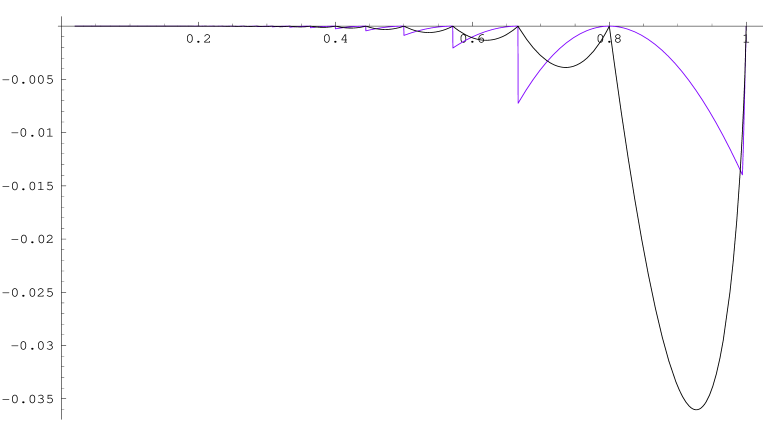
Figure 2: $\mathop{\mathrm{low}}\nolimits_{4,1}-gh_{4}$-black, $\mathop{\mathrm{low}}\nolimits_{4,2}-gh_{4}$-blue, color online

It turns out that for many of the values of $p$, the lower bound $\mathop{\mathrm{low}}\nolimits_{r,2}(p)$ a better lower bound than $\mathop{\mathrm{low}}\nolimits_{r,1}(p)$, and it is very close to the function $gh_{r}(p)$. Figure 2 compares the differences $\mathop{\mathrm{low}}\nolimits_{r,1}(p)-gh_{r}(p)$, plotted in black, and $\mathop{\mathrm{low}}\nolimits_{r,2}(p)-gh_{r}(p)$, plotted in blue, for $r=4$.

From this graph and the graphs for $r=3,6$, which are not plotted here, we conclude that the errors $gh_{r}(p)-ghl_{r}(p),gh_{r}(p)-\mathop{\mathrm{low}}\nolimits_{r,1}(p),gh_{r}(p)-\mathop{\mathrm{low}}\nolimits_{r,2}(p)$ are decreasing monotonically with $r$.

Since $\mathop{\mathrm{low}}\nolimits_{6,2}(0.6814)=.7849602275$ we deduce the inequality

$$h_{3}\geq h_{3}(0.6814)\geq\mathop{\mathrm{low}}\nolimits_{6}(0.6814)\geq\mathop{\mathrm{low}}\nolimits_{6,2}(0.6814)=.7849602275$$

given in §1. Combine Corollary 3.3 with Theorem 3.4 to deduce

      Corollary 3.5

For $3\leq r\in\mathbb{N}$ and $p\in[0,1]$

$$\mathop{\mathrm{low}}\nolimits_{r}(p)\geq\max(\mathop{\mathrm{low}}\nolimits_{r,1}(p),\mathop{\mathrm{low}}\nolimits_{r,2}(p)).$$

4 Monomer-dimer densities for Bethe lattices

Let $\mathbf{T}(r)$ be an infinite $r$-regular tree. Recall that $\mathbf{T}(3)$ is known the Bethe lattice. Clearly, each $\mathbf{T}(r)$ is bipartite. For each $\mathbf{T}(r),r\geq 2$ we construct a convergent sequence $\{G_{n}(r)\}$ in sense of Definition 2.1.

Fix a vertex $O$ in $\mathbf{T}(r)$ and consider all vertices in $\mathbf{T}(r)$ whose distance from $O$ is $n\geq 1$. Then the number of such vertices is $r(r-1)^{n-1}$. Let $A_{1},\ldots,A_{r}$ be the $r$ vertices of distance $1$ from $0$. The number of vertices in $\mathbf{T}(r)$ whose distance from $O$ is exactly $n$ is divided to $r$ classes $\mathcal{A}_{i,n},i=1,\ldots,r$, where the points in $\mathcal{A}_{i,n}$ have distance $n-1$ from $A_{i}$. Let $X_{n}=\cup_{i=1}^{r-1}\mathcal{A}_{i,n}$. Note that $\#X_{n}=\#\mathcal{A}_{r,n+1}=(r-1)^{n}$. Let $V_{n}:=\{O\}\cup_{i,j=1}^{r,n}\mathcal{A}_{i,j}\cup A_{r,n+1}$ Let $H_{n}(r)=(X_{n}\cup\mathcal{A}_{r,n+1},F_{n})$ be an arbitrary $r-1$ regular bipartite graph with the two classes of vertices $X_{n},\mathcal{A}_{r,n+1}$. Let $G_{n}(r)=(V_{n},E_{n})$ where $E_{n}$ are the union of the edge set in the induced graph $\mathbf{T}(r)(V_{n})$ and the set $F$. Note that $G_{n}(r)$ is $r$-regular and bipartite. Then $G_{n}(r),n=1,\ldots,$ converges to $\mathbf{T}(r)$.

Note that $\mathbf{T}(2)$ is isomorphic to the integer lattice $\mathbb{Z}$, and $G_{n}(2)$ is a cycle of length $2(n+1)$ for $n\in\mathbb{N}$. Hence

$$h_{G(\mathbb{Z})}(p)=h_{\{G_{n}(2)\}}(p)=gh_{2}(p)\textrm{ for all }p\in[0,1].$$ (4.1)

In [11] it is shown that $\mathop{\mathrm{low}}\nolimits_{2}(p)=gh_{2}(p)$.

Using the definition $\mathop{\mathrm{low}}\nolimits_{r}(p)$ and the fact that $G_{n}(r)$ are $r$-regular and bipartite we obtain.

      Corollary 4.1

Let $2<r\in\mathbb{N}$. Then

$$h_{\{G_{n}(r)\}}(p)\geq\mathop{\mathrm{low}}\nolimits_{r}(p)\textrm{ for all }p\in[0,1].$$ (4.2)

For more complex models, like the Ising model, it is known that this kind of limit is sensitive to the exact limiting sequence of graphs [18]. It is an interesting problem if equality holds in the above inequality for some choices of random graphs $H_{n}(r)\in\mathcal{G}(2(r-1)^{n},r-1),n\in\mathbb{N}$.

5 An example of sequence of tori

We first discuss a sequence of graphs that give the lower and upper bounds for $h_{d}$ and $h_{d}(1)$ for the graph $G(\mathbb{Z}^{d})$ considered in [12]. Assume that the dimension $d>1$. Let $\mathbf{m}^{\prime}:=(m_{1},\ldots,m_{d-1})\in\mathbb{N}^{d-1}$ be fixed and assume that $m_{i}>3$ for $i=1,\ldots,d-1$. Consider the sequence of $d$-dimensional tori $T((\mathbf{m}^{\prime},n))=(V_{n},E_{n}),n=3,4,\ldots$. Each torus is a $2d$-regular graph. If $m_{1},\ldots,m_{d-1}$ and $n$ are even then $T((\mathbf{m}^{\prime},n))$ is bipartite. The vertex set of $T((\mathbf{m}^{\prime},n))$ is the set $V_{n}:=\langle(\mathbf{m}^{\prime},n)\rangle$. $V_{n}$ can be viewed as composed of $n$ layers of vertices $\langle\mathbf{m}^{\prime}\rangle$. The edges between all vertices $\langle\mathbf{m}^{\prime}\rangle$ in each level $k$ are given as in the $d-1$ dimensional torus $T(\mathbf{m}^{\prime})$. The other edges of $T((\mathbf{m}^{\prime},n))$ are going from level $k$ to level $k+1$ for $k=1,\ldots,n$, where the level $n+1$ is identified with the level $1$. (We also identify level $0$ with the level $n$.) The rule for the edges between the level $k$ and the level $k+1$ is independent of $k$. Thus the vertices $(\mathbf{i}^{\prime},k)$ and $(\mathbf{j}^{\prime},k+1)$ in $V_{n}$ are adjacent if and only if $\mathbf{i}^{\prime}=\mathbf{j}^{\prime}$. The adjacency matrix between the two vertices $\mathbf{i}^{\prime}$ in the level $k$ and $\mathbf{j}^{\prime}$ in the level $k+1$ is given by the $0-1$ matrix $A(\mathbf{m}^{\prime}):=(a_{\mathbf{i}^{\prime}\mathbf{j}^{\prime}})_{\mathbf{i}^{\prime},\mathbf{j}^{\prime}\in\langle\mathbf{m}^{\prime}\rangle}$, which is an identity matrix of order $N=\mathrm{vol}(\mathbf{m}^{\prime})$. For any square matrix $A\in\mathbb{R}^{n\times n}$ we denote by $\mathop{\mathrm{tr}}\nolimits A$ and $\rho(A)$ the trace and the spectral radius of $A$ respectively.

Let us recall first the computation of the monomer-dimer entropy $h_{d}$ given in [12]. The entries of the transfer matrix $B(\mathbf{m}^{\prime})=(b_{ST})_{S,T\subset\langle\mathbf{m}^{\prime}\rangle}$ are indexed by two subsets of $S,T$ of $\langle\mathbf{m}^{\prime}\rangle$. (These subsets may be empty.) First $b_{ST}=0$ if $S\cap T\neq\emptyset$. Second assume that $S\cap T=\emptyset$ then $b_{ST}$ counts the number of the monomer-dimer covers of the subgraph of $T(\mathbf{m}^{\prime})$ induced by the set vertices $\langle\mathbf{m}^{\prime}\rangle\backslash(S\cup T)$. Note that any subgraph of $T(\mathbf{m}^{\prime})$ induced by a set $U\subset\langle\mathbf{m}^{\prime}\rangle$ can be covered by monomers. Hence $b_{ST}\geq 1$. (If $S\cup T=\langle\mathbf{m}\rangle$ then $b_{ST}=1$.) It is not hard to see that the product of $n$ terms $b_{S_{1}S_{2}}b_{S_{2}S_{3}}\ldots b_{S_{n-1}S_{n}}b_{S_{n}S_{1}}$ corresponds to all monomer-dimer covers of $G_{n}=T((\mathbf{m}^{\prime},n))$ with the following conditions. For each level $k=1,\ldots,n$ the dimers going from the level $k$ to $k-1$ are located at the set $S_{k}$ and the dimers going from the level $k$ to the level $k+1$ are located at the set $S_{k+1}$. Let $\Phi(G_{n}):=\sum_{l=0}^{\infty}\phi(l,G_{n})$ number of all possible monomer-dimer covering $T((\mathbf{m}^{\prime},n))$. Then $\mathop{\mathrm{tr}}\nolimits B(\mathbf{m}^{\prime})^{n}=\Phi(G_{n})$. It is shown in [12]

$$\lim_{n\to\infty}\frac{\log\Phi(G_{n})}{\#V_{n}}=\frac{\log\rho(B(\mathbf{m}^{\prime}))}{\mathrm{vol}(\mathbf{m}^{\prime})},\;h_{d}=\lim_{\mathbf{m}^{\prime}\to\infty}\frac{\log\rho(B(\mathbf{m}^{\prime}))}{\mathrm{vol}(\mathbf{m}^{\prime})},$$ (5.1)

$$\texttt{ and }h_{d}\leq\frac{\log\rho(B(2\mathbf{m}^{\prime}))}{\mathrm{vol}(2\mathbf{m}^{\prime})}\texttt{ for any }\mathbf{m}^{\prime}\in\mathbb{N}^{d-1}.$$

(Here $2\mathbf{m}^{\prime}:=(2m_{1},\ldots,2m_{d-1})$.) The lower bounds for $h_{d}$ are also expressed in terms of linear combinations of certain $\log\rho(B(\mathbf{m}^{\prime}))$ corresponding to different values of $\mathbf{m}^{\prime}$.

Let $T((\mathbf{m}^{\prime},\mathbb{Z}))$ be an infinite graph given by the set of vertices $\langle\mathbf{m}^{\prime}\rangle\times\mathbb{Z}$ and the following set of edges $\tilde{E}(\mathbf{m}^{\prime},\mathbb{Z})$. $((\mathbf{i}^{\prime},p),(\mathbf{j}^{\prime},q))\in\tilde{E}(\mathbf{m}^{\prime},\mathbb{Z})$ if either $p=q$ and $(\mathbf{i}^{\prime},\mathbf{j}^{\prime})\in\tilde{E}(\mathbf{m}^{\prime})$ or $|p-q|=1$ and $\mathbf{i}^{\prime}=\mathbf{j}^{\prime}$. Thus the sequence of graphs $G_{n}:=T((\mathbf{m}^{\prime},n)),n=3,4,\ldots$ converges to $G:=T((\mathbf{m}^{\prime},\mathbb{Z}))$. Let $h_{G}(p):=h_{\{G_{n}\}}(p)$ be defined by (2.1-2.2). We now show how to compute $h_{G}(p)$ using the pressure function.

Let $S,T$ be two disjoint subsets of $\langle\mathbf{m}^{\prime}\rangle$. Let $E^{\prime}\subset\tilde{E}(\mathbf{m}^{\prime})$ be an $l$-matching of $T(\mathbf{m}^{\prime})$ so that each edge $(u,v)\in E^{\prime}$ represents a dimer occupying two adjacent vertices in $T(\mathbf{m}^{\prime})$ located in $\langle\mathbf{m}^{\prime}\rangle\backslash(S\cup T)$. To this matching we correspond a monomial $x^{l}$. Let $c_{ST}(x)$ be the sum of all such monomials. $c_{ST}(x)$ is the matching polynomial for the graph $T(\mathbf{m}^{\prime},S,T)$, the subgraph of $T(\mathbf{m}^{\prime})$ induced by the subset of vertices $\langle\mathbf{m}^{\prime}\rangle\backslash(S\cup T)$. We let $c_{ST}(x)=0$ if $S,T\subset\langle\mathbf{m}^{\prime}\rangle$ and $S\cap T\neq\emptyset$. Then $b_{ST}=c_{ST}(1)$. Let $b_{ST}(t):=c_{ST}(e^{2t})e^{(\#S+\#T)t}$ and $B(\mathbf{m},t):=(b_{ST}(t))_{S,T\subset\langle\mathbf{m}^{\prime}\rangle}$. The arguments in [12] that show that $\Phi(G_{n})=\psi(1,G_{n})$ yield the equality $\mathop{\mathrm{tr}}\nolimits B(\mathbf{m},t)^{n}=\psi(e^{2t},G_{n})$. The definition (2.3) of pressure $P(t)$ and the arguments in [12] for the equality (5.1) imply

$$P(t):=P_{\{G_{n}\}}(t)=\frac{\log\rho(B(\mathbf{m},t))}{\mathrm{vol}(\mathbf{m}^{\prime})},\quad t\in\mathbb{R}.$$ (5.2)

(We suppressed the dependence of $P(t)$ on $\mathbf{m}^{\prime}$.)

The following results are known, e.g. [1, 13], and we bring their proof for completeness.

      Theorem 5.1

Let $P(t):=P_{\{G_{n}\}}$ be defined by (5.2). Then $P$ is a smooth increasing convex function on $\mathbb{R}$. Furthermore

$$\lim_{t\to-\infty}P^{\prime}(t)=0,\quad\lim_{t\to\infty}P^{\prime}(t)=1.$$ (5.3)

Let $p(t):=P^{\prime}(t),t\in\mathbb{R}$. Then $p(t)$ is an increasing function such that $p([-\infty,\infty])=[0,1]$. Furthermore

$$h_{\{G_{n}\}}(P^{\prime}(t))=P(t)-tP^{\prime}(t)\texttt{ for any }t\in\mathbb{R},$$ (5.4)

and $h_{\{G_{n}\}}(p)$ is a continuous concave function on $[0,1]$, which is smooth in $(0,1)$.

Proof. The well known result [22] yields $P(t)$ is a convex function of $t$. Since $\mathbf{m}^{\prime}$ is fixed we let $B(t):=B(\mathbf{m}^{\prime},t)$ and $N=\mathrm{vol}(\mathbf{m}^{\prime})$. As $B(t)$ is irreducible, and the nonzero entries of $B(t)$ are increasing function on $\mathbb{R}$, it follows that $P(t)$ increases. Since $\rho(B(t))$ is a simple root positive of the characteristic polynomial it follows that $\rho(B(t))$ and $P(t)$ is an analytic function in some open domain containing $\mathbb{R}$.

$$B(t)=\sum_{i=0}^{N}e^{it}B_{i},\textrm{ each }B_{i}\textrm{ is nonnegative}.$$ (5.5)

$B_{0}=(b_{ST,0})_{S,T\subset\langle\mathbf{m}^{\prime}\rangle}$ corresponds to monomer configurations of . I.e. $B_{0}$ is a diagonal matrix with one nonzero entry $b_{\emptyset\emptyset,0}=1$. The matrix $B_{N}$ corresponds to the tiling of $T((\mathbf{m}^{\prime},n))$ by dimers. Hence $P(t)=\log\rho(B(t))$ is not a linear function. The analyticity of $P(t)$ yields that $P^{\prime\prime}(t)$ may have only finite number of zeros on any closed interval $[a,b]$. The convexity of $P(t)$ implies that $P^{\prime\prime}\geq 0$ on $\mathbb{R}$. Hence $P^{\prime\prime}$ is positive on any $[a,b]$ except a finite number of points. Thus $p(t)=P^{\prime}(t)$ increases on $\mathbb{R}$ and $P(t)$ is strictly convex on $\mathbb{R}$. Let $x=e^{t}$. Then the $\tilde{B}(x):=B(\log x)$ is a polynomial in $x$. Since $\rho(\tilde{B}(0))=\rho(B_{0})=1$ is a simple root of the characteristic polynomial of $B_{0}$ it follows that $\rho(\tilde{B}(x))$ is analytic in some disk $|x|<\epsilon$, such that $|\rho(\tilde{B}(x))|>0$ in this disk. Hence the branch $\log\rho(\tilde{B}(x)),\log\rho(\tilde{B}(0))=0$ is analytic in this disk and has Taylor expansion. The same statement holds for the derivative of $\log\rho(\tilde{B}(x))$. Substitute $x=e^{t}$ to deduce that $P(t)=\frac{\log\rho(\tilde{B}(e^{t}))}{N}$ and its derivative have convergent series in $x=e^{t}$ for $t<-R$, for some $R>>1$. This implies the first equality in (5.3).

Observe that

$$P(t)=t+\frac{\log\rho(\hat{B}(t))}{N},\quad\hat{B}(t):=\sum_{i=0}^{N}e^{(i-N)t}B_{i}.$$

Hence $P^{\prime}(t)=1+(\frac{\log\rho(\hat{B}(t))}{N})^{\prime}$. The arguments above for the first equality in (5.3) imply that the second equality in (5.3).

We now show the inequality

$$P(t)\geq pt+h_{G}(p)\textrm{ for all }p\in[0,1].$$ (5.6)

Let $l_{n}\in[0,n]\cap\mathbb{Z},n\in\mathbb{N}$ be sequence satisfying (2.2). Then

$$\mathop{\mathrm{tr}}\nolimits B(t)^{n}=\psi(e^{2t},G_{n})\geq e^{2l_{n}t}\phi(l_{n},G_{n})\Rightarrow$$

$$\frac{\log\mathop{\mathrm{tr}}\nolimits B(t)^{n}}{Nn}\geq\frac{2l_{n}t}{Nn}+\frac{\log\phi(l_{n},G_{n})}{Nn}.$$

Recall that $\#V_{n}$, the number of vertices in $G_{n}$ is $Nn$. Use the definition of $P(t)$ and (2.2) to deduce

$$P(t)\geq pt+\limsup_{n\to\infty}\frac{\log\phi(l_{n},G_{n})}{\#V_{n}}.$$

Use the definition (2.1-2.2) of $h_{G}(p):=h_{\{G_{n}\}}(p)$ to deduce the inequality (5.6). It is straightforward to show that $h_{G}(p)$ upper semicontinuous on $[0,1]$.

We now show that for each $t\in\mathbb{R}$ there exists $p(t)\in[0,1]$ such that:

$$P(t)\leq p(t)t+h_{G}(p(t)).$$ (5.7)

Let $l_{n}(t)\in[0,\frac{nN}{2}]\cap\mathbb{Z}]$ satisfy

$$e^{2lt}\phi(l,G_{n})\leq e^{2l_{n}(t)t}\phi(l_{n}(t),G_{n}),\textrm{ for }l=0,\ldots\lfloor\frac{nN}{2}\rfloor.$$

Hence

$$\phi(e^{2t},G_{n})\leq\frac{nN}{2}e^{2l_{n}(t)t}\phi(l_{n}(t),G_{n}).$$ (5.8)

Take a subsequence $n_{k},k\in\mathbb{N}$ such that $\lim_{k\to\infty}\frac{\log\psi(e^{2t},G_{n_{k}})}{n_{k}N}=P(t)$. Choose a subsequence $j_{k},k\in\mathbb{N}$ of $n_{k},k\in\mathbb{N}$, such that $\lim_{k\to\infty}\frac{l_{j_{k}}(t)}{j_{k}N}=p(t)\in[0,1]$. Take the logarithm of the inequality (5.8) and divide by $nN$. Let $n=j_{k}$ and let $k\to\infty$. The definition (2.1-2.2) of $h_{G}(p)$ yields the inequality (5.7).

The inequalities (5.6) and (5.7) yield the equality $P(t)=p(t)t+h_{G}(p(t))$. Moreover (5.6) yields $P(y)$ lies above the line $p(t)y+h_{G}(p(t)$, which intersect $P(y)$ at the point $y=t$. Hence $p(t)=P^{\prime}(t)$ and $h_{G}(p(t))=P(t)-p(t)t$. I.e. (5.4) holds. Since $P^{\prime}$ increasing and analytic the implicit function theorem yields that $t=Q(p)$ is analytic in $p\in(0,1)$. Hence $h_{G}(p)$ is analytic on $(0,1)$. Observe that $-h_{G}(p)$ is the Legendre function corresponding to a smooth strictly convex function $P(t)$ [31]. Hence $h_{G}(p)$ is concave on $(0,1)$. Our arguments yield that $h_{G}(p)$ is continuous on $[0,1]$. Hence $h_{G}(p)$ is a concave function on $[0,1]$. $\Box$

      Remark 5.2

Let $h_{G}(p):=h_{\{G_{n}\}}(p)$ and $P(t):=P_{\{G_{n}\}}(t)$ be given as in Definition 2.1. Theorem 5.1 applies to $h_{G}(p)$ and $P(t)$ in the following cases:

1. There exists a nonnegative irreducible matrix $B(t)$ of the form (5.5) such that

   • $\#V_{n}=nN,\;n\in\mathbb{N}$.

   • $\psi(e^{2t},G_{n})=\mathop{\mathrm{tr}}\nolimits B(t)^{n},\;n\in\mathbb{N}$.

   • $\rho(B_{0})=1$ and $\rho(B_{N})$ are positive simple roots the characteristic polynomials of $B_{0}$ and $B_{N}$ respectively.

   2. $G_{n}$ is a disjoint union of $n$ copies of a finite graph $H=(W,F)$ which has a perfect matching. Then $P(t)=\frac{\log\psi(e^{2t},H)}{\#W}$.

6 A construction of sequences of graphs

We now generalize the construction in the previous section to a general construction of a sequence of regular graphs. Let $F=(U,D)$ be an undirected graph with the set of vertices $U$ and the set of edges $D$. For $n\geq 2$ let $G_{n}:=(V_{n},E_{n})$ be the following graph. $V_{n}=U\times\langle n\rangle$, i.e. we can view $V_{n}$ consisting of $n$ copies of $U$ arranged in the $n$ layers $(U,1),(U,2),\ldots,(U,n)$. We let $(U,0):=(U,n),(U,n+1):=(U,1)$. Then

1. For any $u,v\in U$ and $k\in\langle n\rangle$ $((u,k),(v,k))\in E_{n}\iff(u,v)\in D$.

2. Any other edges of $E_{n}$ are between the vertices $(U,k)$ and $(U,k+1)$ for $k=1,\ldots,n$.

3. Let $A=(a_{uv})_{u,v\in U}$ be a given nonzero $0-1$ matrix. Then for each $k\in\langle n\rangle$ $((u,k),(v,k+1))\in E_{n}\iff a_{uv}=1$. We call $A$ the connection matrix.

4. For any two subsets $S,T\subset U$, ($S,T$ may be empty), let $\tilde{a}_{ST}\in\mathbb{Z}_{+}$ be defined as follows. If $\#S\neq\#T$ then $\tilde{a}_{ST}=0$. Assume that $\#S=\#T$. Let $\mathcal{B}(S,T)$ be the set of all bijections $\beta:S\to T$. Then $\tilde{a}_{\emptyset\emptyset}=1$ and $\tilde{a}_{ST}=\sum_{\beta\in\mathcal{B}(S,T)}\prod_{s\in S}a_{s\beta(s)}$ for $\#S=\#T\geq 1$.

   Thus $\tilde{a}_{ST}$ is the number of perfect matchings in the subgraph of the bipartite graph on the set of vertices $(U,1)\cup(U,2)$, and the set edges $E\subset(U,1)\times(U,2)$ given by $A$, and induced by the subset of vertices $(S,1)\cup(T,2)$. Let $\tilde{A}:=(\tilde{a}_{ST})_{S,T\subset U}$ be a $2^{\#U}\times 2^{\#U}$ matrix with nonnegative integer entries.

5. For any two disjoint subsets $S,T\subset U$, let $c_{ST}(x)$ be the matching generating polynomial of the subgraph of $F$ induced by the set of vertices $U\backslash(S\cup T)$. For non-disjoint subset $S,T\subset U$ let $c_{ST}(x)=0$. Let $M(t):=(c_{ST}(e^{2t})e^{(\#S+\#T)t})_{S,T\subset U}$ and $B(t):=M(t)\tilde{A}$ be $2^{\#U}\times 2^{\#U}$ nonnegative matrices for any $t\in\mathbb{R}$. Then $\log\rho(B(t))$ is a continuous convex function on $\mathbb{R}$. If $B(1)$ is an irreducible matrix then $\log\rho(B(t))$ is an analytic function on $\mathbb{R}$. (See arguments of the proof of Theorem 5.2.)

Then the sequence $G_{n},n=2,\ldots$ has the following properties:

• If $F$ is connected then each $G_{n}$ is connected.

• Assume that $F$ is bipartite, where $U=U_{1}\cup U_{2},D\subset U_{1}\times U_{2}$. Suppose that the edges between the two consecutive levels of vertices $(U,k)$ and $(U,k+1)$ are either between $(U_{i},k)$ and $(U_{i},k+1)$ for $i=1,2$ or between $(U_{i},k)$ and $(U_{i+1},k+1)$ for $i=1,2$. ($U_{3}:=U_{1}$.) If $n$ is even then $G_{n}$ is bipartite.

• Assume that $F$ is $p$-regular. Assume that the matrix $A$ has $q$ $1$’s in each row and column. Then $G_{n}$ is $p+2q$-regular graph.

• Assume that $F$ is $p$-regular bipartite. Let $U=U_{1}\cup U_{2},D\subset U_{1}\times U_{2}$ and $n$ is even. Assume that the matrix $A$ has the following properties. Each row indexed by $u\in U_{1}$ and each column indexed by $v\in U_{2}$ has $q$ $1$’s, and each row indexed by $v\in U_{2}$ and each column indexed by $u\in U_{1}$ has $q-1$ $1$’s. ($q\in\mathbb{N}$.) Then $G_{n}$ is $p+2q-1$ regular.

• Then sequence of graphs $G_{n},n=2,3,\ldots$ converges to the infinite graph $G=(V,E)$, where $V=F\times\mathbb{Z}$. The edges $E$ are either between the two vertices on the same level $(U,k),k\in\mathbb{Z}$, determined by $D$, or between the vertices of two consecutive levels $(U,k)$ and $(U,k+1)$, given by the incidence matrix $A$ in the way described above.

• $P(t):=\frac{\log\rho(B(t))}{\#U}$ is the pressure of $G$. Assume that $B(1)$ is an irreducible matrix. Let $h_{G}(p)$ be defined by (2.1-2.2). Then (5.4) holds. (See Remark 5.2.)

In the example of $G_{n}=T((\mathbf{m}^{\prime},n)),n=3,4,\ldots$, discussed in the previous section, we have that $U=T(\mathbf{m}^{\prime})$ and $A$ is the identity matrix $I$. Hence $\tilde{A}$ is also the identity matrix.

7 The upper matching conjecture

For $r\geq 2$ let $K_{r,r}$ be a complete bipartite graph on $2r$ vertices, where each vertex has degree $r$. Then

$$\phi(l,K_{r,r})={r\choose l}^{2}l!,\;l\in\mathbb{Z}_{+},\texttt{ and }\psi(x,K_{r,r})=\sum_{l=0}^{r}{r\choose l}^{2}l!x^{l}.$$ (7.1)

      Conjecture 7.1

( The upper matching conjecture.) Let $G=(V,E)$ be a finite bipartite regular $r$-regular graph on $2qr$ vertices where $2\leq q,r\in\mathbb{N}$. Let $qK_{r,r}$ be the graph consisting of $q$ copies of $K_{r,r}$. Then $\phi(l,G)\leq\phi(l,qK_{r,r})$ for $l=0,\ldots,qr$.

In [11] we proved the above conjecture for $r=2$. We also showed that for $r=2$ $\phi(l,G)\leq\phi(l,qK_{2,2})$ for any $2$ regular graph $G$ on $4q$ vertices. ($G$ does not have to be bipartite.) It is plausible that in the above conjecture one can drop the assumption that $G$ is bipartite. For $l=0,1$ the above conjecture is trivial. For $l=qr$ the above conjecture follows from the Minc conjecture proved by Bregman [3].

Let $K(r)$ be an infinite countable union of $K_{r,r}$. Let $h_{K(r)}(p)$ be defined as in (2.1-2.2) where $G_{n}=nK_{r,r},n\in\mathbb{N}$. Let $G_{n}=(V_{n},E_{n}),n\in\mathbb{N}$ be a sequence of $r$ regular bipartite graphs, where $\#V_{n}\to\infty$. Let $h_{\{G_{n}\}}(p)$ be defined as in (2.1-2.2). Assume for simplicity of the exposition that $\#V_{n}=2q_{n}r$. Then Conjecture 7.1 yields $\phi(l,G_{n})\leq\phi(l,{q_{n}}K_{r,r})$ for $n\in\mathbb{N}$. Hence the UMC yields the AUMC: $h_{G}(p)\leq h_{K(r)}(p)$ for any $p\in[0,1]$.

We use the pressure $P_{K(r)}(t)$, as pointed in Remark 5.2, to compute $h_{K(r)}(p)$. Clearly the matching generating polynomial of $qK_{r,r}$ is $\psi(x,K_{r,r})^{q}$. Hence

$$P_{K(r)}(t)=\frac{\log\sum_{l=0}^{r}{r\choose l}^{2}l!e^{2lt}}{2r},\quad t\in\mathbb{R}.$$ (7.2)

This formula follows also from the results of the previous section, where $F=K_{r,r}$ and the incidence matrix $A$ between two levels $(U,1)$ and $(U,2)$ is the zero matrix. Then $\rho(B(t)\tilde{A})=\psi(e^{2t},K_{r,r})$. (5.4) yields

$$h_{K(r)}(p(t))=\frac{\log\sum_{l=0}^{r}{r\choose l}^{2}l!e^{2lt}}{2r}-\frac{t\sum_{l=0}^{r}{r\choose l}^{2}l!(2l)e^{2lt}}{2r\sum_{l=0}^{r}{r\choose l}^{2}l!e^{2lt}},$$ (7.3)

$$\texttt{where }p(t)=\frac{\sum_{l=0}^{r}{r\choose l}^{2}l!(2l)e^{2lt}}{2r\sum_{l=0}^{r}{r\choose l}^{2}l!e^{2lt}}\texttt{ and }t\in\mathbb{R}.$$

      Conjecture 7.2

( The upper asymptotic matching conjecture.) Let $G_{k}=(V_{k},E_{k}),k\in\mathbb{N}$ be a sequence of $r$ regular bipartite graphs, where $\#V_{k}\to\infty$. Let $h_{\{G_{k}\}}(p)$ be defined as in (2.1-2.2). Let $h_{K(r)}(p)$ be defined by (7.3). Then $h_{\{G_{k}\}}(p)\leq h_{K(r)}(p)$ for any $p\in[0,1]$.

It is plausible to assume that Conjecture 7.2 holds under the assumption that each $G_{n}$ is an $r$-regular graph.

      Theorem 7.3

Let $2\leq r\in\mathbb{N}$ and assume that $G_{n}=(V_{n},E_{n}),n\in N$ is a sequence of $r$-regular bipartite graphs such that $\#V_{n}\to\infty$. Let $h_{\{G_{n}\}}(p),p\in[0,1]$ be defined by (2.1-2.2). Then

$$h_{\{G_{n}\}}(p)\leq\min(\mathop{\mathrm{upp}}\nolimits_{r,1}(p),\mathop{\mathrm{upp}}\nolimits_{r,2}(p))\textrm{ for all }p\in[0,1],$$ (7.4)

where

$$\mathop{\mathrm{upp}}\nolimits_{r,1}(p):=\frac{p\log r!}{2r}-\frac{1}{2}p\log p-(1-p)\log(1-p),$$ (7.5)

$$\mathop{\mathrm{upp}}\nolimits_{r,2}(p):=\frac{p\log r}{2}-\frac{1}{2}\big{(}p\log p+(1-p)\log(1-p)\big{)}.$$ (7.6)

Proof. We claim that for any $G=(V_{1}\cup V_{2},E)\in\mathcal{G}(2m,r)$ the following inequality holds

$$\phi(l,G)\leq{m\choose l}\frac{(m!)^{\frac{m-l}{m}}}{(m-l)!}(r!)^{\frac{l}{r}}.$$ (7.7)

Indeed, let $U_{1}\subset V_{1}$ be a subset of cardinality $l$. Consider the induced bipartite graph $G(U_{1}\cup V_{2})$. Then $G(U_{1}\cup V_{2})$ is also an induced subgraph of the graph $G^{\prime}=(V_{1}\cup V_{2},E^{\prime})$, where the induced subgraph $G^{\prime}(V_{1}\backslash U_{1}\cup V_{2})$ is the complete bipartite graph on $V_{1}\backslash U_{1}\cup V_{2}$. It is straightforward to see that $\phi(l,G^{\prime})=(m-l)!\phi(l,G(U_{1}\cup V_{2})$. The Bregman inequality [3] yields $\phi(l,G^{\prime})\leq(m!)^{\frac{m-l}{m}}(r!)^{\frac{l}{r}}$. Since the number of choices of $U_{1}$ is ${m\choose l}$ we deduce the inequality (7.7). Let $G_{n}=(V_{n},E_{n})\in\mathcal{G}(2m_{n},r),n\in\mathbb{N}$. Let $l_{n}\in[0,m_{n}]\cap\mathbb{Z}$ be a sequence satisfying (2.2). Take the logarithm of the (7.7) divide by $\#V_{n}=2m_{n}$ and let $n\to\infty$ to obtain that $h_{\{G_{n}\}}(d)\leq\mathop{\mathrm{upp}}\nolimits_{r,1}(p)$.

Our next inequality is

$$\phi(l,G)\leq{m\choose l}r^{l}.$$ (7.8)

Let $U_{1}\subset V_{1},\#U_{1}=l$. Since each vertex of $G$ has degree $r$ it follows that each vertex in $U_{1}$ that $\phi(l,G(U_{1}\cup V_{1}))\leq r^{l}$. As one have $n\choose l$ choices of the set $U_{1}$ we obtain (7.8). The above arguments imply that $h_{\{G_{n}\}}(p)\leq\mathop{\mathrm{upp}}\nolimits_{r,2}(p)$. Hence (7.4) holds. $\Box$

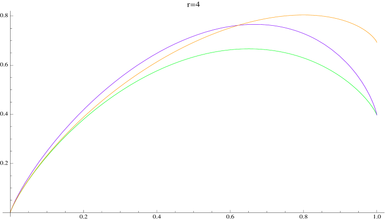
Figure 3: $h_{K(4)}$-green, $\mathop{\mathrm{upp}}\nolimits_{4,1}$-blue, $\mathop{\mathrm{upp}}\nolimits_{4,2}$-orange, color online

Figure 3 gives the plot of $h_{K(r)},\mathop{\mathrm{upp}}\nolimits_{r,1},\mathop{\mathrm{upp}}\nolimits_{r,2}$ for $r=4$. From this graph and the corresponding graphs for $r=3,8$, which is not plotted here, we see that $\min(\mathop{\mathrm{upp}}\nolimits_{r,1}(p),\mathop{\mathrm{upp}}\nolimits_{r,1}(p))-h_{K(r)}(p)$ decreases with $r$. Moreover the intersection point of the graphs $\mathop{\mathrm{upp}}\nolimits_{r,1}$ and $\mathop{\mathrm{upp}}\nolimits_{r,1}$ moves to the left as $r$ increases.

8 Computational results

We have checked the asymptotic matching conjectures for several families like those described in Section 6. In each case we choose $U$ to be a cycle $C_{l}$ of length $l$ for several values of $l$ and then varied the connection matrix $A$. In each case we used the described transfer matrix method to compute the entropy for several values of $p$ and then compared with the conjectured bounds. In all cases the conjectures were found to hold.

In order to test the conjectured lower bound for a given choice of $U$ and $A$ we first constructed the transfer matrix $B(t)$ for the given graph. Given $B(t)$ we can directly compute $P(t)$ from the maximum eigenvalue as in (5.2). Next we computed $P^{\prime}(t)$, using the equality

$$\rho^{\prime}(t)=\eta_{1}^{T}\left(\frac{d}{dt}B(t)\right)\eta_{2},$$

where $\eta_{1}^{T}$ and $\eta_{2}$ are the left and right eigenvectors of $B(t)$, normalized by the condition $\eta_{1}^{T}\eta_{2}=1$. (This is a standard variational formula, e.g. [7].) From these values we now compute $h_{G}(p(t))$ using (5.4). So for each value of $t$ we get a pair $(p(t),h_{G}(p(t)))$ telling us the asymptotic pressure $h_{G}(p(t))$ at the density $p(t)=P^{\prime}(t)$. To make all computations exact we chose $e^{t}$ to be rational numbers, which yielded rational values for all matrix entries.

      Example 8.1 (r=4)

In our first family we let $l$, the length of the cycle $U=C_{l}$, vary from 4 to 8. We tested all permutation matrices $A$, which give every vertex $(u,k)$ in $G_{n}$ one neighbor in the level $k-1$ and one in the level $k+1$, and give rise to a bipartite $G_{n}$. We thus have a family of bipartite 4-regular graphs which includes the standard square lattice tori.

In Figure 4 we plot the difference between the actual values of the entropies $h_{G}(p)$, for all choices of $A$, and the lower asymptotic matching conjecture for a given range of densities $p$. The highest curve correspond to the normal torus graph, i.e it is the graph with the maximum number of matchings of a given size in this family.

      Example 8.2 (r=3)

For our second example we again chose $U=C_{l}$ to be a cycle of length $l$. Here we chose $A$ so that if we number the vertices on the cycle $1,\ldots,l$ the even vertices in the level $k$ have an an odd vertex as a neighbor in the level $k+1$ for $k=1,\ldots,n$. $G_{n}$ is cubic, and for $l$ and $n$ even $G_{n}$ is bipartite. This family includes the torus graphs obtained from the hexagonal lattice which all have girth at least 6. In this case we let the length of the cycle vary from $4$ to 10 and again the conjecture was found to hold. In Figure 5 we display the difference between the actual values of the entropies $h_{G}(p)$, for all choices of $A$, and the lower asymptotic matching conjecture for a given range of densities $p$. Here the values typically stayed closer to the conjecture than for the $4$-regular case, which is to be expected since this graph family has higher girth.

Apart from the above tests, we also tested some more arbitrarily chosen connection matrices giving graphs of degree 6. This was done by $U$ as a cycle and choosing the connection matrix $A$, having two $1$’s in each row and column. Again the conjectures were found to hold but here the deviation up from the conjectured lower bound was even smaller. This is again expected since the conjecture should become more accurate for graphs of higher degree.

9 Infinite graphs with the maximal pressure

In this section we give a partial justification for the computational result in Example 8.1 that the highest curve correspond to the normal torus graph.

      Theorem 9.1

Let $F=(U,D)$ be an undirected graph and consider an infinite graph $G=(V,E)$ defined as follows. $V=U\times\mathbb{Z}$, i.e. the vertices of $G$ consists layers $(U,k),k\in\mathbb{Z}$. The edges $E$ of $G$ connect two vertices on the level $k,j\in\mathbb{Z}$ only if $|k-j|\leq 1$. The edges between any two vertices on level $k$ are given by $D$. The edges between the level $k$ and the level $k+1$ are given by $\#U\times\#U$ permutation matrix $A_{k}=(a_{uv,k})_{u,v\in U}$ for each $k\in\mathbb{Z}$. Thus $((u,k),(v,k+1))\in E\iff a_{uv,k}=1$. Let $M(t),t\in\mathbb{R}$ and $\tilde{A}_{k}$ be the $2^{\#U}\times 2^{\#U}$ nonnegative matrices defined as in §3. Then the pressure $P_{G}(t)$ of $G$ is given as

$$P_{G}(t)=\limsup_{i,j\to\infty}\frac{\log\mathop{\mathrm{tr}}\nolimits M(t)\tilde{A}_{-j}M(t)\tilde{A}_{-j+1}\ldots M(t)\tilde{A}_{i}}{(i+j+1)\#U}.$$ (9.1)

Let $G_{0}$ be the infinite graph obtained by letting $A_{k}$ to be the identity matrix for each $k\in\mathbb{Z}$. Then

$$P_{G_{0}}(t)=\frac{\log\rho(M(t))}{\#U}\geq P_{G}(t)$$ (9.2)

for any $t\in\mathbb{R}$ and any $G$ of the above form. In particular the monomer-dimer entropy $h_{G}$ of $G$, which is equal to $P_{G}(0)$, does not exceed $h_{G_{0}}=P_{G_{0}}(0)$.

Proof. Fix $i,j\in\mathbb{N}$ and let $n=i+j+1$. Define $G_{n}=(V_{n},E_{n})$ to be the following graph. $V_{n}$ consists of $n$ copies of $U$, labelled as $(U,k)$ for $k=-j,\ldots,i$. The edges of $E_{n}$ are induced by the edges of $G$, except that the edges from the level $i$ are connected to the edges of the level $-j$, which is identified with the level $i+1$, by the connection matrix $A_{i}$. The arguments of §2 yield that $\psi(e^{2t},G_{n})=\mathop{\mathrm{tr}}\nolimits M(t)\tilde{A}_{-j}M(t)\tilde{A}_{-j+1}\ldots M(t)\tilde{A}_{i}$. Hence $P_{G}$ is given by (9.1) [13].

Consider now the case of $G_{0}$ where $A_{k}=I$. Then (9.1) yields $P_{G_{0}}(t)=\frac{\log\rho(M(t))}{\#U}$. (See for example [9, §10] for the self-contained details of the arguments on matrices used here.) From the definition of $M(t)$ it follows that $M(t)$ is a nonnegative and symmetric matrix. Hence $\rho(M(t))=||M(t)||$, where $||M(t)||$ is the $l_{2}$ operator norm of $M(t)$. Since $A_{k}$ is a permutation it follows that $\tilde{A}_{k}$ is also a permutation matrix. Hence $||\tilde{A}_{k}||=1$. Thus

$$||M(t)\tilde{A}_{-j}M(t)\tilde{A}_{-j+1}\ldots M(t)\tilde{A}_{i}||\leq||M(t)||^{i+j+1}=\rho(M(t))^{i+j+1}\Rightarrow$$

$$\mathop{\mathrm{tr}}\nolimits M(t)\tilde{A}_{-j}M(t)\tilde{A}_{-j+1}\ldots M(t)\tilde{A}_{i}\leq 2^{\#U}\rho(M(t))^{i+j+1}\Rightarrow$$

$$P_{G}(t)\leq\frac{\log\rho(M(t))}{\#U}.$$

This proves (9.2).

From the definition of monomer-dimer entropy of $G$ [12] it follows that $h_{G}=P_{G}(0)$. Hence $h_{G}\leq h_{G_{0}}$. $\Box$

      Conjecture 9.2

Let the assumptions of Theorem 9.1 hold. Then for any $p\in[0,1]$ $h_{G}(p)\leq h_{G_{0}}(p)$.

Figure 4: Difference between actual entropy and the lower asymptotic matching conjecture for 4-regular graphs with $U=C_{8}$

Figure 5: Difference between actual entropy and the lower asymptotic matching conjecture for 3-regular graphs with $U=C_{10}$

References

• [1] R.J. Baxter, Dimers on a rectangular lattice, J. Math.Β Phys. 9 (1968), 650–654.
• [2] J.A. Bondy and D.J.A. Welsh, A note on the monomer dimer problem, Proc.Β Camb.Β Phil.Β Soc. 62 (1966), 503–505.
• [3] L.M. Bregman, Some properties of nonnegative matrices and their permanents, Soviet Math. Dokl. 14 (1973), 945-949.
• [4] M. Ciucu, An improved upper bound for the 3-dimensional dimer problem, Duke Math.Β J. 94 (1998), 1–11.
• [5] M.E. Fisher, Statistical mechanics of dimers on a plane lattice, Phys.Β Rev. 124 (1961), 1664–1672.
• [6] R.H. Fowler and G.S. Rushbrooke, Statistical theory of perfect solutions, Trans.Β Faraday Soc. 33 (1937), 1272–1294.
• [7] S. Friedland Extremal eigenvalue problems, Bull. Brazilian Math. Soc. 9 (1978), 13-40.
• [8] S. Friedland, A proof of a generalized van der Waerden conjecture on permanents, Lin.Β Multilin.Β Algebra 11 (1982), 107–120.
• [9] S. Friedland, Multi-dimensional capacity, pressure and Hausdorff dimension, Mathematical System Theory in Biology, Communication, Computation and Finance, edited by D. Gilliam and J. Rosenthal, IMA vol. 134, Springer, 2003, 183-222.
• [10] S. Friedland and L. Gurvits, Lower bounds for partial matchings in regular bipartite graphs and applications to the monomer-dimer entropy, Combinatorics, Probability and Computing, 17 (2008), 15 pp.
• [11] S. Friedland, E. Krop and K. MarkstrΓΆm, On the Number of Matchings in Regular Graphs, arXiv:math/0801.2256v1, 15 Jan 2008.
• [12] S. Friedland and U.N. Peled, Theory of Computation of Multidimensional Entropy with an Application to the Monomer-Dimer Problem, Advances of Applied Math. 34(2005), 486-522.
• [13] S. Friedland and U.N. Peled, The pressure associated with multidimensional SOFT, in preparation.
• [14] D.S. Gaunt, Exact series-expansion study of the monomer-dimer problem, Phys.Β Rev. 179 (1969) 174–186.
• [15] J.M. Hammersley, Existence theorems and Monte Carlo methods for the monomer-dimer problem, in Reseach papers in statistics: Festschrift for J. Neyman, edited by F.N. David, Wiley, London, 1966, 125–146.
• [16] J.M. Hammersley, An improved lower bound for the multidimesional dimer problem, Proc.Β Camb.Β Phil.Β Soc. 64 (1966), 455–463.
• [17] J.M. Hammersley, Calculations of lattice statistics, in Proc.Β Comput.Β Physics Con., London: Inst.Β of Phys.Β & Phys.Β Soc., 1970, 1–8.
• [18] O. HΓ€ggstrΓΆm, The random-cluster model on a homogeneous tree, Probab. Theory Related Fields 104 (1996), 231–253.
• [19] J. Hammersley and V. Menon, A lower bound for the monomer-dimer problem, J. Inst.Β Math.Β Applic. 6 (1970), 341–364.
• [20] O.J. Heilmann and E.H. Lieb, Theory of monomer-dimer systems., Comm. Math. Phys. 25 (1972), 190–232.
• [21] P.W. Kasteleyn, The statistics of dimers on a lattice, Physica 27 (1961), 1209–1225.
• [22] J.F.C. Kingman, A convexity property of positive matrices, Quart. J. Math. Oxford Ser. 12 (1961), 283–284.
• [23] C. Kenyon, D.Randall and A. Sinclair, Approximating the number of monomer-dimer coverings of a lattice, J. Stat.Β Phys.Β 83 (1996), 637–659.
• [24] M. Jerrum, Two-dimensional monomer-dimer systems are computationally intractible, J. Stat.Β Phys. 48 (1987), 121–134.
• [25] E.H. Lieb, The solution of the dimer problem by the transfer matrix method, J. Math.Β Phys. 8 (1967), 2339–2341.
• [26] P.H. Lundow, Compression of transfer matrices, Discrete Math. 231 (2001), 321–329.
• [27] P.H. Lundow, Klas MarkstrΓΆm, Exact and Approximate Compression of Transfer Matrices for Graph Homomorphisms, 2006, In press.
• [28] J.F. Nagle, New series expansion method for the dimer problem, Phys.Β Rev. 152 (1966), 190–197.
• [29] C. Niculescu, A new look and Newton’ inequalties, J. Inequal. Pure Appl. Math. 1 (2000), Article 17.
• [30] L. Pauling, J. Amer.Β Chem.Β Soc. 57 (1935), 2680–.
• [31] R. T. Rockafeller, Convex Analysis, Princeton Univ. Press 1970.
• [32] A. Schrijver, Counting $1$-factors in regular bipartite graphs, J. Comb.Β Theory B 72 (1998), 122–135.
Refer to caption