The continuous limit of the Moran process and the diffusion of mutant genes in infinite populations

Abstract

We consider the so called Moran process with frequency dependent fitness given by a certain pay-off matrix. For finite populations, we show that the final state must be homogeneous, and show how to compute the fixation probabilities. Next, we consider the infinite population limit, and discuss the appropriate scalings for the drift-diffusion limit. In this case, a degenerated parabolic PDE is formally obtained that, in the special case of frequency independent fitness, recovers the celebrated Kimura equation in population genetics. We then show that the corresponding initial value problem is well posed and that the discrete model converges to the PDE model as the population size goes to infinity. We also study some game-theoretic aspects of the dynamics and characterize the best strategies, in an appropriate sense.

1 Introduction

Since the beginning of modern evolutionary theory, the study of the dynamics of a mutant gene in a population has attracted attention [10, 11, 15, 37, 38]. It has been known for a long time that a mutant gene will be, eventually, either fixed or lost. The final result depends not only on natural selection but also on chance [20].

The most natural attempt to describe mathematically the evolution of a mutant gene uses a discrete model for a finite population. The question of finding a consistent model for the infinite population is then a natural one. This is called in the physical literature the “thermodynamical limit”, and it is a classical subject on that field. See, for example, [8].

When we consider the infinite population limit, it is natural to have continuous variables where we previously had discrete ones. For example, if $N$ denotes the size of the population, the possible fractions of mutants are $0,1/N,2/N,\cdots,1$. In the limit $N\to\infty$ this fills the entire real interval $[0,1]$. Time should be rescaled accordingly, such that that the probability of fixation, for a given fraction $x$ over a given time span $t$, does not depend significantly on the size of the population. In the infinite limit, we obtain a partial differential equation (PDE). This PDE is an approximation for large $N$ of the discrete process, and as such must present diffusion to the boundaries as a continuous representation of the fact that the mutant gene will be eventually fixed or lost.

A different approach to the same problem is to consider continuous models from the beginning. This leads to two distinct modeling paradigms: the first one uses ordinary differential equations (ODEs) to model the evolution of the fraction of mutants. The most widely used equation in this context is the replicator dynamics and its variations [16]. The second one, which will be further developed in this work, uses PDEs to model the evolutionary process. This approach goes back, at least, to the seminal work by Kimura [20], where it was used to model the diffusion of mutant genes. More explicitly, Kimura considered the probability of fixation of a mutant gene that in a given time is present in a certain fraction of the population. Here, we will deduce the Kimura equation as a particular case of our work, where a PDE will be obtained from the more basic discrete process, in the infinite population limit, for the diffusion of mutant genes.

In this work, we consider a simple evolutionary process, called the Moran process, introduced in [23] (used, e.g., for cancer dynamics [19, 28], paleontology [25], phylogeny [24], genealogy [9], and epidemiology [36]) for a finite population and obtain a partial differential equation as its thermodynamical limit.

Our starting point is evolutionary game theory. We consider a finite population of fully connected interacting individuals through a certain pay-off matrix. We start by proving that for any finite population (of size $N$) of two-types, one of the types will be fixed after long enough time. The thermodynamical limit is then obtained as a PDE that approximates the finite population dynamics for large $N$. We consider two different scalings for the time-step $\Delta t$, namely: $\Delta t=1/N$ (drift limit) and $\Delta t=1/N^{2}$ (drift-diffusion or simply diffusion limit). In the second case it is also important to introduce the so called weak selection limit (pay-offs go to 1, when population goes to infinity). We also show that the most interesting equations appear in the drift-diffusion limit.

All the equations found in the limit are degenerate, i.e., the diffusion coefficient vanishes on the boundaries. The mathematical theory for such equations is not as well developed as for the non-degenerate case. There are the classical books [2, 6]. In particular, [2] proves existence and uniqueness for the equation obtained by Kimura. For more recent works, see also [1, 7].

If we impose no diffusion in the PDE model, the solution can be decomposed in point dynamics, where each fraction evolves through the replicator dynamics. The stationary states and long time behavior of the replicator dynamics are, however, different to the ones obtained as the thermodynamical limit of the final states of discrete populations, showing that the diffusion is essential to understand the discrete dynamics.

The PDE model allows the introduction of a relation of dominance between two different strategists that turns out to be, in its dynamical features, identical to the flow of the replicator dynamics. We also show that the best possible strategy in the finite, but large, population case is given by the evolutionarily stable strategy (ESS) of the game [16, 32]. This clarifies the relation between a homogeneous population playing mixed strategies with given frequencies and a mixed population, with constant fractions, playing pure strategies, i.e., the difference between evolutionarily stable strategies and evolutionarily stable states.

If the fitness for the individuals in the population is frequency independent, the resulting equation is equivalent to a well-know equation of population genetics, introduced by Kimura [20], describing the probability of fixation of a mutant (with frequency independent fitness) in a population. It turns out, that the equation derived in this work and the one introduced by Kimura are a forward/backward pair of equations.

It is important to note that the perception that the Moran process (at least in the frequency independent case) is related to diffusion process is not new [4, 5]. The compatibility between finite populations simulations and the ESS, defined in the continuous case, are also studied in [12, 13, 29].

The structure of this work is the following: In Section 2 we introduce the (finite population) Moran process and study its properties. In particular, we prove that the final state will be always homogeneous. In Section 3 we introduce the drift-diffusion scaling and obtain a PDE as the thermodynamical limit of the Moran process. We also study its dynamic features from the strategic point of view. In Section 4, we consider the no diffusion case and compare the PDE obtained with the replicator dynamics. In Section 5 we particularize all results to the frequency independent case and in Section 6 we study the drift scaling. Finally, in Section 7 we point new directions for this work, showing how the tools developed here can be applied to different dynamics.

2 The frequency dependent discrete case

We consider a fixed size population with two types of individuals: $\mathbb{A}$ and $\mathbb{B}$, say. At fixed time steps, we choose one of the individuals to be eliminated at random and replace it by a newborn which can be of either type. This newborn is obtained as a copy of one of the remaining individuals with probability proportional to its fitness. See Figure 1 for an illustration. This process is called the Moran process [23].

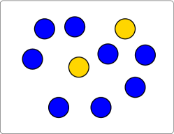
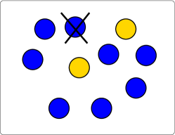
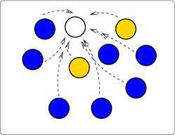
(a)                                       (b)                                       (c)

Figure 1: The Moran process: from a two-types population (a) we chose one at random to kill (b) and a second to copy an paste in the place left by the first, this time proportional to the fitness.

Let $P(t,n,N)$ be the probability that there are $n$ type $\mathbb{A}$ individuals at time $t$ in a population of fixed size $N$. We define $c_{+}(n,N)$ ($c_{0}(n,N)$ and $c_{-}(n,N)$, respectively) as the probability (independent of time) that the number of mutants changes in time $t$ from $n$ to $n+1$ (to $n$ and to $n-1$ respectively) in time $t+\Delta t$. We assume that these transition probabilities are proportional to the fitness $\phi_{A}$ and $\phi_{B}$ of types $\mathbb{A}$ and $\mathbb{B}$ respectively; thus we have:

$$c_{+}(n,N) = \frac{N-n}{N}\frac{n\phi_{A}}{n\phi_{A}+(N-n-1)\phi_{B}}\ ,$$ (1)

$$c_{0}(n,N) = \frac{n}{N}\frac{(n-1)\phi_{A}}{(n-1)\phi_{A}+(N-n)\phi_{B}}+\frac{N-n}{N}\frac{(N-n-1)\phi_{B}}{n\phi_{A}+(N-n-1)\phi_{B}}\ ,$$ (2)

$$c_{-}(n,N) = \frac{n}{N}\frac{(N-n)\phi_{B}}{(n-1)\phi_{A}+(N-n)\phi_{B}}\ .$$ (3)

From that, we may easily write an equation for the evolution of $P$:

$$P(t+\Delta t,n,N) = c_{+}(n-1,N)P(t,n-1,N)+c_{0}(n,N)P(t,n,N)$$ (4)

$$+c_{-}(n+1,N)P(t,n+1,N)\ .$$

After imposing the boundary conditions $P(t,-1,N)=P(t,N+1,N)=0$, $\forall t\geq 0$, we conclude that the previous recursion is valid for $t\geq 0$ and $n=0,1,\cdots,N$.

Originally, the Moran process was defined with a frequency-independent fitness, i.e., $\phi_{A,B}$ were independent of the particular composition of the population. We consider, however, the frequency-dependent case, and we obtain the results for frequency-independent populations as a special case.

Now, we obtain the fitness. For that, we first consider a two players game, with pay-off matrix given by:

	I	II
I	$A$	$B$
II	$C$	$D$

,

where I and II are two pure strategies and $A,B,C,D>0$. We call an $E_{q}$-strategist an individual that plays I with probability $q$ and II with probability $1-q$.

We assume that the two types play two (possibly) different strategies, $E_{q_{1}}$ and $E_{q_{2}}$. The pay-off matrix is then given by

	$E_{q_{1}}$	$E_{q_{2}}$
$E_{q_{1}}$	$\widetilde{A}$	$\widetilde{B}$
$E_{q_{2}}$	$\widetilde{C}$	$\widetilde{D}$

,

where

$$\widetilde{A} := q_{1}^{2}A+q_{1}(1-q_{1})(B+C)+(1-q_{1})^{2}D\ ,$$ (5)

$$\widetilde{B} := q_{1}q_{2}A+q_{1}(1-q_{2})B+(1-q_{1})q_{2}C+(1-q_{1})(1-q_{2})D\ ,$$ (6)

$$\widetilde{C} := q_{1}q_{2}A+(1-q_{1})q_{2}B+q_{1}(1-q_{2})C+(1-q_{1})(1-q_{2})D\ ,$$ (7)

$$\widetilde{D} := q_{2}^{2}A+q_{2}(1-q_{2})(B+C)+(1-q_{2})^{2}D\ .$$ (8)

For simplicity, we consider in this section only pure strategists, i.e., $E_{1}$- and $E_{0}$-strategists for type $\mathbb{A}$ and type $\mathbb{B}$ individuals respectively. The general case follows easily from the results in this section replacing $(A,B,C,D)$ by $(\widetilde{A},\widetilde{B},\widetilde{C},\widetilde{D})$.

We identify fitnesses and pay-offs, and then we have that the fitnesses for I- and II-strategists, for a population with $n$ I-strategists, are given by

$$\phi_{A}=\frac{n-1}{N-1}A+\frac{N-n}{N-1}B\ ,\ \ n=1,\cdots,N\ ,$$ (9)

$$\phi_{B}=\frac{n}{N-1}C+\frac{N-n-1}{N-1}D\ ,\ \ n=0,\cdots,N-1\ .$$ (10)

Then, the evolution iteration is given by Equation (4) with transition coefficients (1)–(3) and (9)–(10).

2.1 The discrete dynamics

A natural question is what are the steady states of the iteration defined by the Moran process. Here we show that the discrete model cannot have a non-pure equilibrium.

Let us define the relative fitness as

$$\rho_{N}(n)=\frac{\phi_{A}(n)}{\phi_{B}(n)}=\frac{(A-B)n+BN-A}{(C-D)n+(N-1)D}>0.$$

Also, let

$$f_{N}(n)=\frac{n}{N}\left(\frac{N-n}{N}\right)\quad\text{and}\quad g_{N}(n,\rho)=\frac{N-1+(\rho-1)n}{N}.$$

Then it is a straightforward computation to verify that

$$c_{+}(n,N)=\frac{f_{N}(n)\rho_{N}(n)}{g_{N}(n,\rho_{N}(n))},\quad c_{-}(n,N)=\frac{f_{N}(n)}{g_{N}(n-1,\rho_{N}(n))}$$

and

$$c_{0}(n,N)=1-f_{N}(n)\left(\frac{\rho_{N}(n)}{g_{N}(n,\rho_{N}(n))}+\frac{1}{g_{N}(n-1,\rho_{N}(n))}\right).$$

Let $\mathbf{M}$ be the iteration matrix of (4). Then $\mathbf{M}$ is a $N+1\times N+1$, tridiagonal matrix, with entries given by

$$\mathbf{M}_{ii}=c_{0}(i,N),\quad i=0,\ldots,N,$$

$$\mathbf{M}_{(i+1)i}=c_{+}(i,N)\quad\text{and}\quad\mathbf{M}_{i(i+1)}=c_{-}(i+1,N),\quad i=0,\ldots,N-1.$$

From this, and the fact that $\rho_{N}(n)>0$, it is easy to see that $\mathbf{M}$ is a nonnegative matrix. Since $c_{0}(n,N)+c_{+}(n,N)+c_{-}(n,N)=1$, $\mathbf{M}$ is column stochastic.

The answer to question raised in the beginning of this section is given by the following result:

Proposition 1.

Let $\mathbf{M}$ be as above and let $\mathbf{P(t)}=(P(t,0),P(t,1),\ldots,P(t,N))^{\dagger}$. Then

1. $$\lim_{k\to\infty}\mathbf{M}^{k}=\begin{pmatrix}1&1-F_{1}&\ldots&1-F_{N-1}&0\\ 0&0&\ldots&\ldots&0\\ \vdots&\vdots&\vdots&\vdots&\vdots\\ 0&0&\ldots&\ldots&0\\ 0&F_{1}&\ldots&F_{N-1}&1\end{pmatrix},$$

   where the $F_{n}$ satisfy

   $$F_{n}=c_{+}(n,N)F_{n+1}+c_{-}(n,N)F_{n-1}+c_{0}(n,N)F_{n},$$

   $$F_{0}=0\quad\text{and}\quad F_{N}=1.$$ (11)

2. If $\mathbf{1}$ denotes the vector $(1,1,\ldots,1)^{\dagger}$, $\mathbf{F}=(F_{0},F_{1},\ldots,F_{N})^{\dagger}$ and if $\langle\cdot,\cdot,\rangle$ denotes the usual inner product, then we have that

   $$\langle\mathbf{P}(t),\mathbf{1}\rangle=\langle\mathbf{P}(0),\mathbf{1}\rangle\quad\text{and}\quad\langle\mathbf{P(t)},\mathbf{F}\rangle=\langle\mathbf{P(0)},\mathbf{F}\rangle.$$

   In particular, the $l^{1}$-norm of a nonnegative initial condition is preserved.

Proof.

For part 1, see the proof at appendix A.

As for part 2, we first observe that, if a vector $\mathbf{V}$ satisfies $\mathbf{M}^{\dagger}\mathbf{V}=\mathbf{V}$, then we have that

$$\langle\mathbf{P(t+\Delta t)},\mathbf{V}\rangle=\langle\mathbf{M}\mathbf{P(t)},\mathbf{V}\rangle=\langle\mathbf{P(t)},\mathbf{M}^{\dagger}\mathbf{V}\rangle=\langle\mathbf{P(t)},\mathbf{V}\rangle.$$

Hence

$$\langle\mathbf{P}(t),\mathbf{V}\rangle=\langle\mathbf{P}(0),\mathbf{V}\rangle.$$

From the fact that $\mathbf{M}$ is column stochastic, we easily conclude that

$$\mathbf{M}^{\dagger}\mathbf{1}=\mathbf{1},$$

and the first invariant follows. For the second invariant, we observe that Equation (11) can be written in matrix notation as

$$\mathbf{M}^{\dagger}\mathbf{F}=\mathbf{F},$$

which concludes the proof. ∎

Remark 1.

The two invariants described in part 2 of the proposition 1 are the only invariants of the Moran process and play an important role in the determination of the correct continuous solution.

Thus, the equilibrium states must have their mass concentrated in the extremes. The $F_{n}$ turns out to be the fixation probability of I-strategists, when the process start with $n$ I-strategists.

From the definitions of $c_{*}(n,N)$, we see that $F_{n}$ satisfies:

$$\left\{\begin{array}[]{rcl}&&\rho_{N}(n)F_{n+1}-\left(\rho_{N}(n)+\frac{g_{N}(n,\rho_{N}(n))}{g_{N}(n-1,\rho_{N}(n))}\right)F_{n}+\frac{g_{N}(n,\rho_{N}(n))}{g_{N}(n-1,\rho_{N}(n))}F_{n-1}=0\ ,\\ &&F_{0}=0\quad\text{and}\quad F_{N}=1.\end{array}\right.$$ (12)

Equation (12) can be solved by writing

$$H(n)=\frac{g_{N}(n,\rho_{N}(n))}{\rho_{N}(n)g_{N}(n-1,\rho_{N}(n))}\quad\text{and}\quad G_{n}=F_{n}-F_{n-1}$$

Then, ignoring the boundary conditions for the moment, we have that

$$G_{n+1}=H(n)G_{n},$$

with solution given by

$$G_{n}=G_{1}\prod_{i=1}^{n-1}H(i).$$

Since

$$F_{n}-F_{n-1}=G_{1}\prod_{i=1}^{n-1}H(i),$$

we obtain, after applying $F_{N}=1$ and $F_{0}=0$, that:

$$F_{n} =G_{1}\sum_{k=1}^{n}\prod_{i=1}^{k-1}H(i),$$

$$G_{1} =\left(\sum_{k=1}^{N}\prod_{i=1}^{k-1}H(i)\right)^{-1}.$$ (13)

The expression given by (13) does not appear to yield a simple formula in the general case. However, compare the formulas found in Section 5, where we study the case when the relative fitness is constant with respect to $n$.

Remark 2.

The coefficients obtained in the above analysis are for a Death/Birth process. For a Birth/Death process, they are simpler and are given by

$$c_{+}(n,N) = \frac{f_{N}(n)\rho_{N}(n)}{\tilde{g}_{N}(n,\rho_{N}(n))}\ ,$$

$$c_{-}(n,N) = \frac{f_{N}(n)}{\tilde{g}_{N}(n,\rho_{N}(n))}\ ,$$

$$c_{0}(n,N) = 1-\frac{f_{N}(n)}{\tilde{g}_{N}(n,\rho_{N}(n))}\left(1+\rho_{N}(n)\right)\,$$

where

$$\tilde{g}_{N}(n,\rho)=\frac{N+(\rho-1)n}{N}.$$

Also, in this case $H(n)$ simplifies to

$$H(n)=\frac{1}{\rho_{N}(n)}.$$

2.2 Numerical Results

We numerically computed the $\mathbf{M}^{10000}$, for $N=20$ and various relative fitnesses. The entries predicted to be zero by Proposition 1 were found to have magnitude less than $10^{-50}$.

Also, from these calculations, we extracted the fixation probabilities and compared them with the ones obtained by evaluating (13) numerically. The result for a specific choice of fitness is displayed in Figure 2.

Figure 2: Fixation probabilities for $N=20$, $A=2$, $B=1$, $C=3$ and $D=1$. The points are taken from $\mathbf{M}^{10000}$, while the lines are obtained by numerically solving (13).

For the case of frequency independent fitness, we can obtain explicit formulas for the fixation probability— see Section 5 — and we also compare with the fixation probabilities extracted from $\mathbf{M}^{10000}$ in Figure 3.

(a)                                                            (b)

Figure 3: Fixation probabilities for constant $r=C/A=D/B$, when $N=20$ computed from $\mathbf{M}^{10000}$ together with the analytical fixation plotted as continuous functions of $n/N$; (a) $r=1$ (b) $r=1.5$.

3 The thermodynamical limit

The aim of this section is to derive a continuous approximation, i.e., a PDE model for the discrete process described in the previous section.

We define the probability density that at time $t$ we have a fraction $x\in[0,1]$ of type $\mathbb{A}$ individuals

$$\mathcal{P}(t,x,N):=\frac{P(t,xN,N)}{\frac{1}{N}}=NP(t,xN,N)\;,\quad\text{with}\quad x=\frac{n}{N},\quad n=0,1,2,\ldots,N.$$

Furthermore, we assume that in the limit $N\to\infty$, $\mathcal{P}(t,x,N)$ converges in some sense to a function $p(t,x)$ which is sufficiently smooth so that

$$p\left(t,x\pm\frac{1}{N}\right)=p(t,x)\pm\frac{1}{N}\partial_{x}p(t,x)+\frac{1}{2N^{2}}\partial_{x}^{2}p(t,x)+{\mathcal{O}}(N^{-3})$$ (14)

and re-write equation (4) to second order in $N^{-1}$ as

$$p(t+\Delta t,x)-p(t,x)=\frac{1}{N}\left[\left(c_{+}^{(1)}+c_{0}^{(1)}+c_{-}^{(1)}\right)p-\left(c_{+}^{(0)}-c_{-}^{(0)}\right)\partial_{x}p\right]$$ (15)

$$\qquad+\frac{1}{N^{2}}\left[\frac{1}{2}\left(c_{+}^{(2)}+c_{0}^{(2)}+c_{-}^{(2)}\right)p-\left(c_{+}^{(1)}-c_{-}^{(1)}\right)\partial_{x}p+\frac{1}{2}\left(c_{+}^{(0)}+c_{-}^{(0)}\right)\partial_{x}^{2}p\right]$$

$$\qquad+{\mathcal{O}}\left(\frac{1}{N^{3}}\right)\ ,$$

where $c_{*}^{(i)}=c_{*}^{(i)}(x)$, $*=+,0,-$, $i=0,1,2$, are defined by

$$c_{+}\left(\left(x-\frac{1}{N}\right)N,N\right) = c_{+}(n-1,N)=c_{+}^{(0)}+\frac{1}{N}c_{+}^{(1)}+\frac{1}{2N^{2}}c_{+}^{(2)}\ ,$$ (16)

$$c_{0}(xN,N) = c_{0}(n,N)=c_{0}^{(0)}+\frac{1}{N}c_{0}^{(1)}+\frac{1}{2N^{2}}c_{0}^{(2)}\ ,$$ (17)

$$c_{-}\left(\left(x+\frac{1}{N}\right)N,N\right) = c_{-}(n-1,N)=c_{-}^{(0)}+\frac{1}{N}c_{-}^{(1)}+\frac{1}{2N^{2}}c_{-}^{(2)}\ .$$ (18)

Then

$$c_{+}^{(1)}+c_{0}^{(1)}+c_{-}^{(1)} = \left(Ax^{2}+D(1-x)^{2}+(B+C)x(1-x)\right)^{-2}\cdot\bigl{[}A(A-C)x^{4}$$

$$+\left(B(B-D)+C(C-A)+2C(B-D)\right)x^{2}(1-x)^{2}$$

$$+D(D-B)(1-x)^{4}+2x(1-x)\left(A(B-D)x^{2}-(A-C)D(1-x)\right)\bigr{]}\ ,$$

$$c_{+}^{(0)}-c_{-}^{(0)} = \frac{x(1-x)\left(x(A-C)+(1-x)(B-D)\right)}{Ax^{2}+D(1-x)^{2}+(B+C)x(1-x)}\ ,$$ (20)

If we impose that

$$\lim_{N\to\infty}(A,B,C,D)=(1,1,1,1)\ ,$$ (21)

$$\lim_{N\to\infty}N(A-1,B-1,C-1,D-1)=(a,b,c,d)\ ,$$ (22)

we find

$$\lim_{N\to\infty}\left(c_{+}^{(2)}+c_{0}^{(2)}+c_{-}^{(2)}\right) = -4\ ,$$

$$\lim_{N\to\infty}\left(c_{+}^{(1)}-c_{-}^{(1)}\right) = -2+4x\ ,$$

$$\lim_{N\to\infty}\left(c_{+}^{(0)}+c_{-}^{(0)}\right) = 2x(1-x)\ ,$$

and, from (3–20), we have

$$\lim_{N\to\infty}N\left(c_{+}^{(1)}+c_{0}^{(1)}+c_{-}^{(1)}\right) = -3x^{2}(a-b-c+d)-2x(a-c-2(b-d))+(d-b)\ ,$$

$$\lim_{N\to\infty}N\left(c_{+}^{(0)}-c_{-}^{(0)}\right) = x(1-x)(x(a-c)+(1-x)(b-d))\ .$$

Finally, we divide Equation (15) by $\Delta t=N^{-2}$ (diffusive scaling), and take the limit $N\to\infty$, to obtain

$$\partial_{t}p = \left[3x^{2}(a-b-c+d)-2x(a-c-2(b-d))-(b-d)\right]p$$

$$-x(1-x)(x(a-c)+(1-x)(b-d))\partial_{x}p$$

$$+(-2)p+2(1-2x)\partial_{x}p+x(1-x)\partial_{x}^{2}p$$

i.e.,

$$\partial_{t}p=\partial_{x}^{2}\left[x(1-x)p\right]-\partial_{x}\left[x(1-x)(x\alpha+(1-x)\beta)p\right]\ .$$ (23)

where $\alpha=a-c$ and $\beta=b-d$. We also define $\eta=\alpha-\beta$.

Supplementing Equation (23) we have the following conservation laws:

$$\frac{{\mathrm{d}}}{{\mathrm{d}}t}\int_{0}^{1}p(t,x){\mathrm{d}}x=0\quad\text{and}\quad\frac{{\mathrm{d}}}{{\mathrm{d}}t}\int_{0}^{1}\psi(x)p(t,x){\mathrm{d}}x=0,$$

where $\psi(x)$ is given in Theorem 2.

Remark 3.

It is important to stress that if we do not impose conditions (21)–(22), there are another possible scalings. More precisely, if (21) still holds but (22) is replaced by

$$\lim_{N\to\infty}N^{\nu}(A-1,B-1,C-1,D-1)=(a,b,c,d),\qquad 0<\nu<1,$$

then another possible scaling is given by taking $\Delta t=(1/N)^{1+\nu}$ and, in this case, we obtain (23) without the diffusion term. This equation is discussed in Section 4. Moreover, if we drop (21)–(22), and only require that the payoffs have a finite limit when $N$ goes to infinity, then yet another scaling is given by $\Delta t=1/N$ and, in this case, the equation for the probability density is given by

$$\partial_{t}\bar{p}=\partial_{x}\left[\frac{x(1-x)\left(x(A-C)+(1-x)(B-D)\right)}{x^{2}(A-B-C+D)+x(B+C-2D)+D}\bar{p}\right]\ .$$ (24)

We analyze this equation in Section 6.

Equation (23) is not readily covered by the usual theory of parabolic PDEs. However, the analysis can be extended to obtain the following result:

Theorem 1.

1. For a given $p^{0}\in L^{1}([0,1])$, there exists a unique solution $p=p(t,x)$ to Equation (34) of class $C^{\infty}\left(\mathbb{R}^{+}\times(0,1)\right)$ that satisfies $p(0,x)=p^{0}(x)$.

2. The solution can be written as

   $$p(t,x)=q(t,x)+a(t)\delta_{0}+b(t)\delta_{1},$$

   where $q\in C^{\infty}(\mathbb{R}^{+}\times[0,1])$ satisfies (23) without boundary conditions, and we also have

   $$a(t)=\int_{0}^{t}q(s,0){\mathrm{d}}s\quad\text{and}\quad b(t)=\int_{0}^{t}q(s,1){\mathrm{d}}s.$$

   In particular, we have that $p\in C^{\infty}(\mathbb{R}^{+}\times(0,1))$.

3. We also have that

   $$\lim_{t\to\infty}q(t,x)=0\text{ (uniformly)},\quad\lim_{t\to\infty}a(t)=\pi_{0}[p^{0}]\quad\text{and}\quad\lim_{t\to\infty}b(t)=\pi_{1}[p^{0}],$$

   where $\pi_{0}$ and $\pi_{1}$ are computed in Theorem 2. Note that this means that the solution solution will ’die out’ in the interior and only the Dirac masses in the extremities will survive.

4. Assume $p^{0}\in L^{2}([0,1])$ and let $J(t)=\int_{0}^{1}x(1-x)q^{2}(t,x){\mathrm{d}}x$. Then, we have that

   $$J(t)\leq J(0)e^{-2\lambda_{0}t},\lambda_{0}>0.$$

See the proof at Appendix B.

For completeness we show various numerical simulations for computing $p(t,x)$. Due to display convenience we plot $P(t,x)=(\Delta x)p(t,x)$, instead of $p(t,x)$. See Figures 4–12.

We observe that $p^{\prime}(t,x)=p(t,1-x)$ also satisfies (23) changing the parameters $(\alpha,\beta)\to(-\beta,-\alpha)$. Hence each computation actually yields solution for two set of parameters, just by reflecting the solution around the axis $x=1/2$.

Figure 4: Solutions for $P(t,x)$ for various times, when $\beta=\alpha=0$. This is the pure diffusive constant fitness case. Note the diffusion to the boundaries. The initial condition is given by $p^{0}(x)=\delta_{1/2}(x)$.

Figure 5: Solutions for $P(0.1,x)$ for various values $\beta$ and $\eta:=\alpha-\beta$. Here, the initial condition is the same as in Figure 4.

Figure 6: Solutions for $P(t,x)$ when $\beta=2$ and $\eta=0$ for various times. This is the case of some drift with constant fitness. The initial condition is $p^{0}(x)=20x^{3}(1-x)$, which is asymmetric with a peak at $x=3/4$. Notice that the form of the initial condition together with the drift sign leads to a very rapid convergence to the equilibrium state.

Figure 7: Solutions for $P(t,x)$ for various times, when $\beta=2$ and $\eta=1$. The initial condition is the same as in in figure 6. Notice that there is little difference from the computation with $\eta=0$ thanks to the form of the initial condition and to the order one size of the parameters.

Figure 8: Same as Figure 7, but with $\beta=1$ and $\eta=2$. Same remarks apply in this case.

Figure 9: Solutions for $P(t,x)$ for various times when $\beta=10$ and $\eta=20$ with the same initial condition as in Figure 6. The convergence for the equilibrium state is very fast also in this case.

Figure 10: Solutions for $P(t,x)$ for various times when $\beta=-20$ and $\eta=-40$. In this case the drift forces the solution to accumulate in the opposite direction of the initial large concentration.

Figure 11: Solutions for $P(t,x)$ for various times when $\beta=20$ and $\eta=-40$. Here, the convective term vanishes at $x=1/2$. The effect is that, at first, the solution convected until the its peak reaches $x=1/2$. Then it essentially stays there, while diffusion enforces the transport to the boundaries. In the second figure, the very ends of the interval are omitted for better view of the behavior in interior.

Figure 12: Solutions for $P(t,x)$ for various times, when $\beta=-20$ and $\eta=40$, with initial condition $p^{0}(x)=6x(1-x)$. In this case, the sign of $\eta$ drives the solution out of $x=1/2$ to the extremes. The initial condition was chosen to be symmetric in this case to highlight this behavior. Also, as in the previous example, the second figure have the very ends of the interval omitted for a better view of the inner behavior.

Notice that, for $\alpha-\beta,\beta\gg 1$, we expect a behavior drift-dominated for intermediate times. This means that, if $x^{*}=\beta/(\beta-\alpha)\not\in(0,1)$, then the solution will be convected until it reaches one of the boundaries, and then will diffuse to the steady state. Otherwise, depending on the sign of $\eta$ the solution will either first concentrate near $x^{*}$, and then diffuses to the boundary, or depart from $x^{*}$ in both directions towards the ends. Notice also, that the solutions are never smooth at the ends. Computations with different values of $\alpha$ and $\beta$ produces qualitatively similar graphics.

Now, let us go back to the general case, i.e., for $E_{q_{1}}$- and $E_{q_{2}}$-strategists, instead of only pure strategists. Then, in a straightforward way (see also Equations (5)–(8)), we define

$$\tilde{a} := q_{1}^{2}a+q_{1}(1-q_{1})(b+c)+(1-q_{1})^{2}d\ ,$$

$$\tilde{b} := q_{1}q_{2}a+q_{1}(1-q_{2})b+(1-q_{1})q_{2}c+(1-q_{1})(1-q_{2})d\ ,$$

$$\tilde{c} := q_{1}q_{2}a+(1-q_{1})q_{2}b+q_{1}(1-q_{2})c+(1-q_{1})(1-q_{2})d\ ,$$

$$\tilde{d} := q_{2}^{2}a+q_{2}(1-q_{2})(b+c)+(1-q_{2})^{2}d\ .$$

Then, the equation for $p$, the fraction of $E_{q_{1}}$-strategists in the population is given by

$$\partial_{t}p = \partial_{x}^{2}\left(x(1-x)p\right)-\partial_{x}\left(x(1-x)(x(\tilde{a}-\tilde{c})+(1-x)(\tilde{b}-\tilde{d}))p\right)$$ (25)

$$= \partial_{x}^{2}\left(x(1-x)p\right)-\partial_{x}\left(x(1-x)(x(\tilde{\alpha}+(1-x)\tilde{\beta}))p\right)\ ,$$

where $\tilde{\alpha}:=\tilde{a}-\tilde{c}=(q_{1}-q_{2})(q_{1}\alpha+(1-q_{1})\beta)$ and $\tilde{\beta}:=\tilde{b}-\tilde{d}=(q_{1}-q_{2})(q_{2}\alpha+(1-q_{2})\beta)$. Note that $\tilde{\alpha}-\tilde{\beta}=(q_{1}-q_{2})^{2}(\alpha-\beta)$. Then, if $q_{1}\not=q_{2}$ and $\alpha\not=\beta$, then $\tilde{\alpha}\not=\tilde{\beta}$.

Theorem 2.

For $p(0,\cdot)=p^{0}\in L_{+}^{1}\cap L^{\infty}([0,1])$, the solution of Equation (25) is unique, non-negative, and accumulates on the boundaries, i.e., $p^{\infty}:=\lim_{t\to\infty}p=\pi_{0}[p^{0}]\delta_{0}+\pi_{1}[p^{0}]\delta_{1}$, where $\pi_{0}[p^{0}]=1-\pi_{1}[p^{0}]$ and the fixation probability of $E_{q_{1}}$ strategists is given by

$$\pi_{1}[p^{0}] = \frac{\int_{0}^{1}\left[\int_{y}^{1}p^{0}(x){\mathrm{d}}x\right]\exp\left(-y^{2}(q_{1}-q_{2})^{2}\frac{\alpha-\beta}{2}-y(q_{1}-q_{2})(q_{2}\alpha+(1-q_{2})\beta)\right){\mathrm{d}}y}{\int_{0}^{1}\exp\left(-y^{2}(q_{1}-q_{2})^{2}\frac{\alpha-\beta}{2}-y(q_{1}-q_{2})(q_{2}\alpha+(1-q_{2})\beta)\right){\mathrm{d}}y}$$

$$= \frac{\int_{0}^{1}\int_{0}^{x}p^{0}(x)\exp\left(-y^{2}(q_{1}-q_{2})^{2}\frac{\alpha-\beta}{2}-y(q_{1}-q_{2})(q_{2}\alpha+(1-q_{2})\beta)\right){\mathrm{d}}y\ dx}{\int_{0}^{1}\exp\left(-y^{2}(q_{1}-q_{2})^{2}\frac{\alpha-\beta}{2}-y(q_{1}-q_{2})(q_{2}\alpha+(1-q_{2})\beta)\right){\mathrm{d}}y}\ .$$

Proof.

It is enough to prove for $q_{1}=1$ and $q_{2}=0$ (i.e., for Equation (23)) and then change the result from $(\alpha,\beta)$ to $(\tilde{\alpha},\tilde{\beta})$. Existence, non-negativeness and convergence to the boundaries follows from Theorem 1.

To obtain values $\pi_{i}[p^{0}]$, $i=1,2$, we multiply Equation (23) by $\psi(x)$ and integrate from 0 to 1. On assuming that $p$ is such that integration by parts can be performed and that no boundary terms arise, we obtain that

$$\partial_{t}\int_{0}^{1}p(t,x)\psi(x){\mathrm{d}}x=\int_{0}^{1}x(1-x)p(t,x)\left(\psi^{\prime\prime}(x)+(x(\alpha-\beta)+\beta)\psi^{\prime}(x)\right){\mathrm{d}}x\ .$$

Conservation laws are obtained solving $\psi^{\prime\prime}(x)+(x(\alpha-\beta)+\beta)\psi^{\prime}(x)=0$. Solutions are given by $\psi=\text{cte}$ (conservation of probability) and

$$\psi(x)=c^{-1}\int_{0}^{x}\exp\left(-y^{2}\frac{\alpha-\beta}{2}-y\beta\right){\mathrm{d}}y,\quad\quad c=\int_{0}^{1}\exp\left(-y^{2}\frac{\alpha-\beta}{2}-y\beta\right){\mathrm{d}}y\ .$$

Remark 4.

Notice that $\psi(x)$ is the continuous counterpart to the discrete fixation probabilities.

Using that

$$\int_{0}^{1}p^{0}(x)\psi(x){\mathrm{d}}x=\int_{0}^{1}\left(\pi_{0}[p^{0}]\delta_{0}+\pi_{1}[p^{0}]\delta_{1}\right)\psi(x){\mathrm{d}}x$$

we get

$$\pi_{1}[p^{0}] = \frac{\int_{0}^{1}\left[\int_{y}^{1}p^{0}(x){\mathrm{d}}x\right]\exp\left(-y^{2}\frac{\alpha-\beta}{2}-y\beta\right){\mathrm{d}}y}{\int_{0}^{1}\exp\left(-y^{2}\frac{\alpha-\beta}{2}-y\beta\right){\mathrm{d}}y}\ ,$$

$$= \frac{\int_{0}^{1}\int_{0}^{x}p^{0}(x)\exp\left(-y^{2}\frac{\alpha-\beta}{2}-y\beta\right){\mathrm{d}}y{\mathrm{d}}x}{\int_{0}^{1}\exp\left(-y^{2}\frac{\alpha-\beta}{2}-y\beta\right){\mathrm{d}}y}\ .$$

Finally, we change from $\alpha$, $\beta$ to $\tilde{\alpha}$, $\tilde{\beta}$. ∎

Corollary 1.

If $p^{0}=\delta_{x^{0}}$, then

$$\pi_{1}[\delta_{x^{0}}]=\frac{\int_{0}^{x_{0}}\exp\left(-y^{2}(q_{1}-q_{2})^{2}\frac{\alpha-\beta}{2}-y(q_{1}-q_{2})(q_{2}\alpha+(1-q_{2})\beta)\right){\mathrm{d}}y}{\int_{0}^{1}\exp\left(-y^{2}(q_{1}-q_{2})^{2}\frac{\alpha-\beta}{2}-y(q_{1}-q_{2})(q_{2}\alpha+(1-q_{2})\beta)\right){\mathrm{d}}y}\ .$$

Definition 1.

We say that $E_{q_{2}}$ dominates $E_{q_{1}}$ ($E_{q_{2}}\succ E_{q_{1}}$) if, for any initial condition $p^{0}\in L^{1}_{+}\cap L^{\infty}([0,1])$, the probability of fixation for the strategy $E_{q_{1}}$ is smaller than the one for the neutral case (the case $q_{1}=q_{2}$), i.e.,

$$\pi_{1}[p^{0}]<\pi_{1}^{\mathrm{N}}[p^{0}]:=\int_{0}^{1}xp^{0}(x){\mathrm{d}}x\ .$$

We also say that $E_{q_{2}}$ $\delta$-dominates $E_{q_{1}}$ if the above formula is valid for all $p^{0}=\delta_{x^{0}}$, $x^{0}\in(0,1)$, i.e.,

$$\pi_{1}[\delta_{x^{0}}]=\frac{\int_{0}^{x}F_{(q_{1},q_{2})}(y){\mathrm{d}}y}{\int_{0}^{1}F_{(q_{1},q_{2})}(y){\mathrm{d}}y}<x^{0}\,\ \ \forall x^{0}\in(0,1)\ ,$$ (26)

where we defined the auxiliary function

$$F_{(q_{1},q_{2})}(y):=\exp\left(-y^{2}(q_{1}-q_{2})^{2}\frac{\alpha-\beta}{2}-y(q_{1}-q_{2})(q_{2}\alpha+(1-q_{2})\beta)\right)\ .$$ (27)

The following lemma shows that the two definitions above are in fact equivalent:

Lemma 1.

$E_{q_{2}}$ $\delta$-dominates $E_{q_{1}}$ if and only if $E_{q_{2}}\succ E_{q_{1}}$.

Proof.

We only need to prove the only if case. Let us consider any initial condition given by $p^{0}\in L^{1}_{+}\cap L^{\infty}([0,1])$. Then

$$\pi_{1}[p^{0}] = \frac{\int_{0}^{1}\int_{y}^{1}p^{0}(x)F_{(q_{1},q_{2})}(y){\mathrm{d}}x{\mathrm{d}}y}{\int_{0}^{1}F_{(q_{1},q_{2})}(y){\mathrm{d}}y}$$

$$= \frac{\int_{0}^{1}\int_{y}^{1}\int_{0}^{1}p^{0}(z)\delta(z-x)F_{(q_{1},q_{2})}(y){\mathrm{d}}z{\mathrm{d}}x{\mathrm{d}}y}{\int_{0}^{1}F_{(q_{1},q_{2})}(y){\mathrm{d}}y}$$

$$= \frac{\int_{0}^{1}\int_{0}^{1}\int_{y}^{x}p^{0}(z)\delta(z-x)F_{(q_{1},q_{2})}(y){\mathrm{d}}y{\mathrm{d}}z{\mathrm{d}}x}{\int_{0}^{1}F_{(q_{1},q_{2})}(y){\mathrm{d}}y}$$

$$= \int_{0}^{1}\int_{0}^{1}p^{0}(z)\delta(z-x)\frac{\int_{0}^{x}F_{(q_{1},q_{2})}(y){\mathrm{d}}y}{\int_{0}^{1}F_{(q_{1},q_{2})}(y){\mathrm{d}}y}{\mathrm{d}}z{\mathrm{d}}x\ .$$

Now, we use Equation (26) and conclude that

$$\pi_{1}[p^{0}]<\int_{0}^{1}\int_{0}^{1}p^{0}(z)\delta(z-x)x{\mathrm{d}}z{\mathrm{d}}x=\int_{0}^{1}p^{0}(x)x{\mathrm{d}}x=\pi_{1}^{\mathrm{N}}[p^{0}]\ .$$

∎

In view of this lemma, from now on, we consider only initial conditions of $\delta$-type, i.e., $p^{0}=\delta_{x^{0}}$. In order to prove dominance relations, we prove first the following:

Lemma 2.

If $F_{(q_{1},q_{2})}$ is increasing in the interval $[0,1]$, then $E_{q_{2}}\succ E_{q_{1}}$.

Proof.

For $p^{0}=\delta_{x^{0}}$, Equation (26) can be re-written as

$$\frac{1}{x^{0}}\int_{0}^{x^{0}}F_{(q_{1},q_{2})}(y){\mathrm{d}}y<\int_{0}^{1}F_{(q_{1},q_{2})}(y){\mathrm{d}}y\ ,\ \ \forall x^{0}\in(0,1)\ .$$

This equation can be interpreted as saying that the average of the function $F_{(q_{1},q_{2})}$ in any interval $[0,x^{0}]$, $x^{0}\in(0,1)$ is less than the average in the interval $[0,1]$, which is true whenever the function is increasing. ∎

Finally we prove the full relations of dominance for a $2\times 2$ game.

Theorem 3.

Let $E_{q_{1}}$ and $E_{q_{2}}$, $q_{1},q_{2}\in[0,1]$, be two strategists in a $2\times 2$ game, and let $q^{*}=\beta/(\beta-\alpha)$. Then the relation of dominance is given by Table 1.

		$E_{q_{2}}\succ E_{q_{1}}$ if and only if
$\alpha>\beta>0$	$q^{*}<0$	$q_{2}>q_{1}$
$\alpha>0>\beta$	$q^{*}\in(0,1)$	$q_{2}<q_{1}\leq q^{*}$ or $q_{2}>q_{1}\geq q^{*}$
$0>\alpha>\beta$	$q^{*}>1$	$q_{2}>q_{1}$
$0>\beta>\alpha$	$q^{*}<0$	$q_{2}<q_{1}$
$\beta>0>\alpha$	$q^{*}\in(0,1)$	$q_{1}<q_{2}\leq q^{*}$ or $q_{1}>q_{2}\geq q^{*}$
$\beta>\alpha>0$	$q^{*}>1$	$q_{2}>q_{1}$.

Table 1: Dominance relations for the non-degenerated ($\alpha\not=\beta\not=0\not=\alpha$) thermodynamical limit of the frequency-independent Moran process, given by Equation (25), with $q^{*}=\beta/(\beta-\alpha)$.

Proof.

The proof consists in a long and tedious calculation proving that, for each range in Table 1, the function $F_{(q_{1},q_{2})}$ is increasing. Then we use Lemma 2. ∎

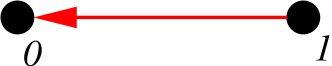
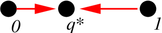
Figure 13: Relation of dominance between $E_{q_{1}}$– and $E_{q_{2}}$–strategists for given parameters. Here, $q^{*}=\beta/(\beta-\alpha)$. The first 2 figures (above) show dominance from pure strategies, the third one ($\alpha>0>\beta$, below, left) shows that the pure strategies dominates their neighbors (and everybody dominates $E_{q^{*}}$) and the last one ($\beta>0>\alpha$, below, right) shows that $E_{q^{*}}$ dominates any strategy. The arrow points from the dominated to the dominant.

The following corollary shows that the strategy $E_{q^{*}}$ is the best possible strategy if $\beta>0>\alpha$.

Corollary 2.

If $\beta>0>\alpha$, then $E_{q^{*}}\succ E_{q}$, $\forall q\not=q^{*}:=\beta/(\beta-\alpha)\in(0,1)$.

Proof.

For $q_{2}=q^{*}$, $F_{(q,q^{*})}$ simplifies for

$$F_{(q,q^{*})}(y)=\exp\left(-y^{2}(q-q^{*})^{2}\frac{\alpha-\beta}{2}\right)\ .$$

For $\alpha-\beta<0$, this is an increasing function of $y$ and this proves the corollary. ∎

In order to finish the full picture of dominance, we need also the following:

Lemma 3.

If $E_{q_{2}}\succ E_{q_{1}}$, then $E_{q_{1}}\not\succ E_{q_{2}}$.

Proof.

First, we see, from Equation (27), that

$$F_{(q_{1},q_{2})}(y)=F_{(q_{2},q_{1})}(1-y)F_{(q_{1},q_{2})}(1)\ .$$

Then, we write

$$\frac{1}{x^{0}}\int_{0}^{x^{0}}F_{(q_{1},q_{2})}(y){\mathrm{d}}y=\frac{1}{x^{0}}\left[\int_{0}^{1}F_{(q_{2},q_{1})}(y){\mathrm{d}}y-\int_{0}^{1-x^{0}}F_{(q_{2},q_{1})}(y){\mathrm{d}}y\right]F_{(q_{1},q_{2})}(1)\ .$$

Furthermore,

$$\int_{0}^{1}F_{(q_{1},q_{2})}(y){\mathrm{d}}y=\int_{0}^{1}F_{(q_{2},q_{1})}(y){\mathrm{d}}yF_{(q_{1},q_{2})}(1)\ .$$

Using the fact that $E_{q_{2}}\succ E_{q_{1}}$, we find

$$\frac{1}{x^{0}}\left[\int_{0}^{1}F{(q_{2},q_{1})}(y){\mathrm{d}}y-\int_{0}^{1-x^{0}}F_{(q_{2},q_{1})}(y)\right]<\int_{0}^{1}F_{(q_{2},q_{1})}(y){\mathrm{d}}y\ .$$

We re-arrange the terms and conclude that

$$\frac{1}{1-x^{0}}\int_{0}^{1-x^{0}}F_{(q_{2},q_{1})}(y){\mathrm{d}}y>\int_{0}^{1}F_{(q_{2},q_{1})}(y){\mathrm{d}}y\ .$$

∎

Table 1, together with Lemma 3 can be summarized in Figure 13.

It is important to note also that in some references (see, e.g., [33]) it is said that selection favors strategy II replacing strategy I (in this case, we say that strategy II weakly dominates strategy I), in a finite population of size $N$, if a single type II mutant has fixation probability larger than $1/N$, the neutral probability. Unfortunately, no sound generalization of this concept can have a graph similar to the one presented in Fig. 13, as it is possible that $E_{q_{2}}$ weakly dominates strategy $E_{q_{1}}$ and vice-versa. See [33] for details.

The concept explained above clearly extend the concept of ESS for the PDE case. As the PDE case works as an approximation for large $N$ of the discrete case, it is easy to see that we can extend the ESS definition also to the more realistic discrete case.

Different to the most known ODE (see also the next section) case for the definition of ESS, here we cannot guarantee that the probability distribution will, in the long range (when adequately parametrized) accumulate in the ESS (when it is in the interior of the interval $[0,1]$), but we can see that an individual that plays strategy I and II with frequencies given by the game’s ESS is optimized to win any contest (with the same parameters).

If the strategists involved in the game play with frequencies different from the ESS (for example, the pure strategies) the ODE prediction is that a stable mixture will evolve. This is impossible in the discrete case (as, in the long range, all individuals will descend of a single one in time $t=0$, which will be of one of the given types) and also in the PDE model (as shown by Theorem 2).

More generally, we say

Theorem 4.

Let $p_{N,\Delta t}(x,t)$ be the solution of the finite population dynamics (of population $N$, time step $\Delta t=1/N^{2}$), with initial conditions given by $p^{0}_{N}(x)=p^{0}(x)$, $x=0,1/N,2/N,\cdots,1$, for $p^{0}\in L^{1}_{+}([0,1])$. Assume also that $(A-1,B-1,C-1,D-1)=1/N(a,b,c,d)+{\mathcal{O}}(1/N^{2})$. Let $p(t,x)$ be the solution of the continuous model with initial condition given by $p^{0}(x)$. If we write $p_{i}^{n}$ for the $i$-th component of $p_{N,\Delta t}(x,t)$ in the $n$-th iteration, we have, for any $t^{*}>0$, that

$$\lim_{N\to\infty}p^{tN^{2}}_{xN}=p(t,x),\quad x\in[0,1],\quad t\in[0,t^{*}].$$

Proof.

First, we consider the matrix $\widetilde{\mathbf{M}}$ obtained from $\mathbf{M}$ by deleting the first and last rows and columns. Then, we observe that the derivation of the thermodynamical limit shows that the discrete iteration given by $\widetilde{\mathbf{M}}$ is consistent — in the approximation sense [30] — with Equation (23), without any boundary conditions, provided that we set $A=1+a/N$, and similarly for $B$, $C$ and $D$. From the results of Appendix A, we know that the discrete iteration is stable, since $\sigma(\widetilde{\mathbf{M}})\subset(-1,1)$. From Appendix B, we see that the continuous problem without boundary conditions is well posed in the $D_{s}$ spaces defined there. In this case, we can then invoke the Lax-Ricthmyer equivalence theorem [30] to guarantee that the discrete model converges to the continuum one, in the limit $\Delta t,\Delta x\to 0$, with $\Delta t=(\Delta x)^{2}$. More precisely, the iteration defined by $\widetilde{\mathbf{M}}$ converges to $q(t,x)$, the smooth part of $p(t,x)$; cf. appendix B

Now returning to the iteration defined by $\mathbf{M}$. In order to finish the proof, we only need to show that $P(t,0)$ and $P(t,1)$ converges weakly to the appropriate Dirac masses. We shall do the computation for $x=0$, the case $x=1$ being similar.

For $x=0$ the iteration defined by $\mathbf{M}$ reads

$$P(t+\Delta t,0)=P(t,0)+\frac{1}{N}P\left(t,\frac{1}{N}\right)$$

Thus, letting $t=0$ and solving the recursion, we have that

$$P(m\Delta t,0)=P(0,0)+\frac{1}{N}\sum_{j=1}^{m-1}P\left(j\Delta t,\frac{1}{N}\right).$$

Since $\mathbf{e}_{1}\in\mathbb{R}^{N}$ converges weakly to $\delta_{0}$ as $N\to\infty$—by considering test functions with support contained in $(1/N,1/N)$—we need only to show that it has the correct mass at each time $t$. For this, notice that

$$\mathcal{P}\left(j\Delta t,\frac{1}{N}\right)=\mathcal{P}\left(j\Delta t,0\right)+\frac{1}{N}\partial_{x}\mathcal{P}\left(j\Delta t,0\right).$$

Since $p(t,x)=N\mathcal{P}(t,x)$, we find that, in a weak sense,

$$\lim_{N\to\infty}p^{tN^{2}}_{0}\to\int_{0}^{t}q(s,0){\mathrm{d}}s+P(0,0).$$

∎

4 The diffusionless case and the replicator dynamics

We shall see in this Section that the ODE Replicator dynamics is equivalent to the diffusionless version of Equation (25). This will have important consequences that we shall discuss later on. Notice also, cf. Remark 3, that this is the correct limiting equation, if the payoffs decay slowly to one as $N\to\infty$.

Thus, we consider

$$\partial_{t}p=-\partial_{x}\left(x(1-x)(x(a-c)+(1-x)(b-d))p\right)\ .$$

A weak solution of this equation is given by $p(t,x)=\delta_{X(t)}$, if $X(t)$ solves

$$\dot{X}=X(1-X)(X(a-c)+(1-X)(b-d))\ ,$$ (28)

which is the simplest replicator equation [16] for the two-person game with pay-off matrix given by

$$\left(\begin{matrix}a&b\\ c&d\end{matrix}\right)\ .$$ (29)

The stationary points of Equation (28) are given by $0$, $1$ and $X^{*}:=\beta/(\beta-\alpha)$. The most interesting scenario occurs when $\alpha<\beta$ and $X^{*}\in(0,1)$ (i.e, $\beta>0>\alpha$): in this case the only stable equilibrium is the non-trivial $X=X^{*}$. For the full analyze, see Table 2. Compare also with the description of dominance in the previous section.

		stable	unstable
$\alpha>\beta>0$	$X^{*}<0$	$X=1$	$X=0$
$\alpha>0>\beta$	$X^{*}\in(0,1)$	$X=0$ and $1$	$X=X^{*}$
$0>\alpha>\beta$	$X^{*}>1$	$X=0$	$X=1$
$0>\beta>\alpha$	$X^{*}<0$	$X=0$	$X=1$
$\beta>0>\alpha$	$X^{*}\in(0,1)$	$X=X^{*}$	$X=0$ and $1$
$\beta>\alpha>0$	$X^{*}>1$	$X=1$	$X=0$

Table 2: Stable and unstable equilibria in the range $[0,1]$ for the non-degenerated ($\alpha\not=\beta\not=0\not=\alpha$) replicator dynamics (28)

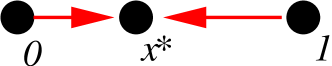
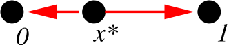
Figure 14: Flux of the replicator equation for pure strategy dominated games (above), mixed strategy dominated (below, left) and bistable games (below, right). Here, $X^{*}=\beta/(\beta-\alpha)$. Compare with Figure 13.

Our definition of dominance seems more general than many definitions that appear in the literature [26, 27, 31, 33]. Furthermore, the use of the thermodynamical limit in the analysis make it much more simple to work. In particular, consider a game between $E_{q_{1}}$- and $E_{q_{2}}$-strategists and a given replicator dynamics such that any non-trivial initial conditional converges in $t\to\infty$ to one of the two trivial equilibria, say, $X=0$. The replicator dynamics is given by

$$\dot{X}=X(1-X)(X(q_{1}-q_{2})^{2}(\alpha-\beta)+(q_{1}-q_{2})(q_{2}\alpha+(1-q_{2})\beta))\ .$$ (30)

If, for any initial condition $X(0)\in(0,1)$, $\lim_{t\to\infty}X(t)=0$, then, $\dot{X}(t)<0$, $\forall X\in(0,1)$, $\forall t\in\mathbb{R}^{+}$, i.e., $(X(q_{1}-q_{2})^{2}(\alpha-\beta)+(q_{1}-q_{2})(q_{2}\alpha+(1-q_{2})\beta))<0$. This implies that $F^{\prime}_{(q_{1},q_{2})}(y)>0$, $\forall y\in(0,1)$, where $F_{(q_{1},q_{2})}$ is defined by Equation (27). In particular $F_{(q_{1},q_{2})}$ is increasing and then from Lemma 2, we have $E_{q_{2}}\succ E_{q_{1}}$. If, on the other hand, $\lim_{t\to\infty}X(t)=1$, by a similar argument, we have that $E_{q_{1}}\succ E_{q_{2}}$.

These picture is completed after looking to Figures 13 and 14 and noting that the flow of the replicator dynamics always goes from the less-dominant strategy to the more dominant one, if we consider an equivalence (at the replicator dynamics level) between mixed populations of pure strategist and populations of mixed strategists.

In reference [35] a thermodynamical limit of a frequency-dependent Moran process was also designed, but the pay-off were not re-scaled when $N\to\infty$ and the Fokker-Planck equation obtained was claimed to be valid for large, but finite $N$, and not in the thermodynamical limit.

5 The Frequency Independent Moran Process

In order to consider frequency-independent fitness, we impose a pay-off matrix such that the gain of a player is independent of others player’s strategies, that is, $A=B$ and $C=D$. In particular, we impose $C/A=D/B=r$. The number $r$ is know as the relative fitness. Most results here are simple corollaries of results from the previous section. We state them only for completeness.

Corollary 3.

The fixation probabilities $F_{n}$ of type $\mathbb{A}$ individuals for an initial condition of $n$ mutants in the frequency independent Moran process with relative fitness $r$ are given by

$$F_{n}=\frac{1-r^{n}}{1-r^{1-N}}+\frac{k}{N}\frac{r^{n}-r^{1-n}}{1-r^{1-N}}\ ,$$ (31)

$$F_{n}=\frac{n}{N}\ ,\ \ r=1\ .$$ (32)

Proof.

When the relative fitness is constant, i.e. $\rho_{N}(n)=1/r$, (13) becomes

$$F_{n} =G_{1}\sum_{k=1}^{n}\frac{1}{\rho^{k-1}}\left(1+\frac{(\rho-1)(k-1)}{N-1}\right),$$

$$G_{1} =\left[\sum_{k=1}^{N}\frac{1}{\rho^{k-1}}\left(1+\frac{(\rho-1)(k-1)}{N-1}\right)\right]^{-1}$$ (33)

We sum the series and prove the corollary. If $r=1$, it is straightforward to see that $F_{n}=n/N$.

∎

Remark 5.

In the case of birth/death process we have instead:

$$F_{n}=G_{1}\sum_{k=1}^{n}\frac{1}{\rho^{k-1}}=G_{1}\sum_{k=1}^{n}r^{k-1}=G_{1}\frac{1-r^{k}}{1-r}=\frac{1-r^{k}}{1-r^{N}}\ ,$$

where we used that

$$G_{1}=\frac{1-r}{1-r^{N}}.$$

Note that the coefficients obtained in Corollary 3 are different from the one obtained in [21], which are the same as in Remark 5. The difference is the result of differences between a death/birth and birth/death processes. Anyhow, the formulas are equivalent for large $N$.

We also define $\gamma:=\alpha=\beta$ and then Equation (25) is

$$\partial_{t}p=\partial_{x}^{2}\left(x(1-x)p\right)-\gamma\partial_{x}\left(x(1-x)p\right)\ .$$ (34)

As a simple consequence of Theorem 2 for Equation (34), we have

Corollary 4.

Let $p$ be a solution of Equation (34) with initial conditions $p^{0}\in L^{1}_{+}\cap L^{\infty}([0,1])$. Then, in a weak sense, $p^{\infty}:=\lim_{t\to\infty}p(\cdot,t)=\pi_{0}[p^{0}]\delta_{0}+\pi_{1}[p^{0}]\delta_{1}$. Furthermore, we have $\pi_{0}[p^{0}]=1-\pi_{1}[p^{0}]$ and

$$\pi_{1}[p^{0}]=\frac{1-\int_{0}^{1}{\mathrm{e}}^{-\gamma x}p^{0}(x){\mathrm{d}}x}{1-e^{-\gamma}}\ .$$

If we start with $p^{0}=\delta_{x_{0}}$, then

$$f_{\gamma}(x_{0}):=\pi_{1}[\delta_{x_{0}}]=\frac{1-{\mathrm{e}}^{-\gamma x_{0}}}{1-{\mathrm{e}}^{-\gamma}}\ ,$$ (35)

and $\lim_{\gamma\to 0}\pi_{1}[\delta_{x_{0}}]=x_{0}$. This is true because the neutral case corresponds to $\gamma=0$. Note that $f_{\gamma}(0)=0$, $f_{\gamma}(1)=1$, $\forall\gamma$ and that $f_{\gamma}(x_{0})\geq x_{0}$ if and only if $\gamma\geq 0$. So, in the language of previous sections, $\mathbb{A}\succ\mathbb{B}\iff\gamma>0$.

It is important to compare the probability of fixation in the continuous limit, Equation (35), and the result obtained for finite population, Equation (31). To understand the idea we should consider that, in the finite case, we have initially a fixed proportion $\kappa\in(0,1)$ of mutants, such that the probability of fixation is given by

$$\frac{1-r^{\kappa N}}{1-r^{N-1}}-\kappa\frac{r^{\kappa N}-r^{\kappa N-1}}{1-r^{N-1}}\approx\frac{1-r^{\kappa N}}{1-r^{N}}\ ,$$

when $N$ is large and $r$ close to 1. To be more precise, if $r(N)=1+\gamma/N$,

$$\lim_{N\to\infty}\frac{\frac{1-r^{\kappa N}}{1-r^{N-1}}-\kappa\frac{r^{\kappa N}-r^{\kappa N-1}}{1-r^{N-1}}}{\frac{1-r^{\kappa N}}{1-r^{N}}}=1\ .$$

In order to compare that formula with (35) for large $N$, we need only to impose $k=x_{0}$ (the initial fraction of mutants) and then ${\mathrm{e}}^{-\gamma}\approx r^{-N}$, i.e., $\gamma\approx N(r-1)$, for $r-1\ll 1$ (valid for large $N$), in agreement with $\gamma=\lim_{N\to\infty}N(r-1)$ (compare with (22)).

We cannot avoid the comparison of our result with the classical results by Kimura [20]. Following this reference, let $u(t,y)$ be the probability that a mutant allele, initially with frequency $y$ and relative fitness $s$ be fixed after a time $t$ in a randomly mating diploid population of size $N_{0}$. Then

$$\partial_{t}u=\frac{y(1-y)}{4N_{0}}\partial_{y}^{2}u+sy(1-y)\partial_{y}u\ .$$ (36)

This equation and Equation (34) are associated backward/forward Kolmogorov equations with suitable rescalings [14]. Then, for example, Equation (35) is the same found in [20], where $\gamma=4Ns$ for $s=r(N)-1$ is the selective advantage. Furthermore, the fact that $f_{0}(x_{0})=x_{0}$ reproduces the idea that a neutral mutant ($\gamma=0$) is fixed with probability equal to its initial frequency.

Following, again, reference [14], if $u(t,y)$ solves Equation (36), then $u(t,x)=u_{\mathrm{S}}(x)p(x,t)$ where

$$u_{\mathrm{S}}(x)=\frac{1-{\mathrm{e}}^{-N_{0}sx}}{1-{\mathrm{e}}^{-4N_{0}s}}$$

is the stationary solution of Equation (36) and $p(x,t)$ solves (34) (with appropriate rescalings and normalizations). This shows the equivalence of this deduction and Kimura’s one.

6 The drift limit

The “drift limit” means that the time-step is re-scaled according to $\Delta t=1/N$. In this case, we do not need to consider the weak selection limit, i.e., pay-offs (and fitness) are considered time-step independent. This problem is mathematically well posed, but, as explained below, it seems not to be an interesting limit from the modeling point of view. We state it only for completeness.

First, we see what happens for the drift limit of the frequency dependent Moran process, i.e., Equation (24).

Theorem 5.

Let $\bar{p}$ be the solution of Equation (24) with initial conditions given by $\bar{p}^{0}\in L^{1}_{+}\cap L^{\infty}([0,1])$. Then, $\bar{p}^{\infty}=\bar{\pi}_{0}\delta_{0}+\bar{\pi}_{*}\delta_{x^{*}}+\bar{\pi}_{1}\delta_{1}$, where $\bar{\pi}_{0}+\bar{\pi}_{*}+\bar{\pi}_{1}=1$ and $x^{*}=-(B-D)/(A-B-C+D)$. Furthermore, if $A-C<0$, then $\bar{\pi}_{0}=0$; if $B-D>0$ then $\bar{\pi}_{1}=0$; and if $(AD-BC)/((A-C)(B-D))<0$ then $\bar{\pi}_{*}=0$. If $x^{*}\not\in[0,1]$, $\bar{\pi}_{*}=0$.

Proof.

We multiply Equation (24) by

$$\psi(x)=(1-x)^{A/(A-C)}x^{-D/(B-D)}(x(A-B-C+D)+B-D)^{(DA-BC)/((A-C)(B-D))}$$

and integrate from 0 to 1. Then

$$\partial_{t}\int_{0}^{1}\psi(x)\bar{p}(x,t){\mathrm{d}}x = -\int_{0}^{1}\frac{x(1-x)(x(A-B-C+D)+B-D)}{x^{2}(A-B-C+D)+x(B+C-2D)+D}\psi^{\prime}(x)\bar{p}(x,t){\mathrm{d}}x$$

$$= -\int_{0}^{1}\psi(x)\bar{p}(x,t){\mathrm{d}}x\ .$$

From Gronwall’s inequality, we find that $\bar{p}^{\infty}$ is supported at the zeros of $\psi(x)$. ∎

Suppose that we have a game where the strategy I dominates (e.g., the Prisoner’s dilemma, where strategy I means “defect”), i.e., $A>C$ and $B>D$. If $AD-BC>0$, $\bar{\pi}_{*}=0$, and if $AD-BC<0$, then $x^{*}>1$, and this implies $\bar{\pi}_{*}=0$. Eventually, the full population will play strategy I.

For $A<C$ and $B<D$, the full population will play strategy II.

For the Hawk-and-Dove game we have $A-C<0$ and $B-D>0$. This implies that $(AD-BC)/((A-C)(B-D))>0$ and then $\bar{p}^{\infty}=\delta_{x^{*}}$, where $x^{*}\in(0,1)$.

Finally, for coordination games, $A-C>0$ and $B-D<0$, then $(AD-BC)/((A-C)(B-D))<0$ and $\bar{p}^{\infty}=\bar{\pi}_{0}\delta_{0}+\bar{\pi}_{1}\delta_{1}$. To obtain the values $\bar{\pi}_{i}$, $i=0,1$, note that $x^{*}\in(0,1)$ and

$$\partial_{t}\int_{0}^{x^{*}}\bar{p}{\mathrm{d}}x=0\ ,\ \ \partial_{t}\int_{x^{*}}^{1}\bar{p}{\mathrm{d}}x=0.$$

This implies that

$$\bar{\pi}_{0} = \int_{0}^{x^{*}}\bar{p}^{\infty}{\mathrm{d}}x=\int_{0}^{x^{*}}\bar{p}^{0}{\mathrm{d}}x\ ,$$

$$\bar{\pi}_{1} = \int_{x^{*}}^{1}\bar{p}^{\infty}{\mathrm{d}}x=\int_{x^{*}}^{1}\bar{p}^{0}{\mathrm{d}}x\ .$$

In a pictorial way, all the mass to the right of $x^{*}$ will move toward the point $x=1$, while the mass on the left will move toward 0. If the initial condition is of delta-type, i.e., $p^{0}=\delta_{x^{0}}$ then the final condition is fully determined, $\bar{p}^{\infty}=\delta_{0}$ ($\bar{p}^{\infty}=\delta_{1}$) if $x_{0}<x^{*}$ ($x_{0}>x^{*}$, respectively).

Now, we consider the frequency independent case, i.e., we impose $A=B=1$ and $C=D=r$ at Equation (24).

Corollary 5.

Let $\bar{p}$ be the solution of

$$\partial_{t}\bar{p}=-(r-1)\partial_{x}\left[\frac{x(1-x)}{x(r-1)+1}\bar{p}\right]\ .$$ (37)

with $\bar{p}^{0}\in L^{1}_{+}\cap L^{\infty}([0,1])$. Then $\bar{p}^{\infty}=\delta_{1}$ for $r>1$ and $\bar{p}^{\infty}=\delta_{0}$ for $r<0$.

Proof.

Note that $\psi(x)=(1-x)^{1/(1-r)}x^{-r/(1-r)}$. Then, its zeros are at most 0 and 1. This implies $\bar{\pi}_{*}=0$. The values of $\bar{\pi}_{0}$ and $\bar{\pi}_{1}$ follow trivially. ∎

As a conclusion of this corollary, we note that the time-step of order $1/N$ implies in no diffusion, i.e., no genetic drift. So, the result of Equation (37) is deterministic, in the sense that an arbitrarily small fraction of advantageous mutant will eventually take over the entire population, while disadvantageous mutants will certainly be extinct (if the population is initially mixed). In Equation (34) nothing similar happens.

7 Final Remarks

The procedure used here can be applied to different evolution process. For example, consider the imitation dynamics given by the following rules: from a population with size $N$ and two possible types, we choose two individuals $I_{1}$ and $I_{2}$. If they are of the same type, nothing changes. If $I_{1}$ is of type $\mathbb{A}$ and $I_{2}$ of type $\mathbb{B}$, $I_{1}$ changes its type with probability $\Psi(\phi_{B}-\phi_{A})$ and the same if we swap $I_{1}$ and $I_{2}$, where $\phi_{A}$ and $\phi_{B}$ are the fitness for the types $\mathbb{A}$ and $\mathbb{B}$ respectively and $\Psi:\mathbb{R}\to[0,1]$ is a continuously differentiable non decreasing function. Then, the transition coefficients are given by

$$c_{+}(n,N) = \frac{N-n}{N}\frac{n}{N-1}\Psi(\phi_{A}-\phi_{B})\ ,$$

$$c_{-}(n,N) = \frac{n}{N}\frac{N-n}{N-1}\Psi(\phi_{B}-\phi_{A})\ ,$$

$$c_{0}(n,N) = 1-c_{+}(n,N)-c_{-}(n,N)\ .$$

We consider the functions of $x=n/N$ as defined in (16)–(18) and with assumptions (21)–(22) we get

$$\lim_{N\to\infty}N\left(c_{1}^{(1)}+c_{0}^{(1)}+c_{-}^{(1)}\right) = 6x^{2}\Psi^{\prime}(0)(a-b-c+d)$$

$$+4x\Psi^{\prime}(0)(-a+2b+c-2d)-2\Psi^{\prime}(0)(b-d)\ ,$$

$$\lim_{N\to\infty}N\left(c_{+}^{(0)}-c_{-}^{(0)}\right) = -2x^{3}\Psi^{\prime}(0)(a-b-c+d)$$

$$-2x^{2}\Psi^{\prime}(0)(-a+2b+c-2d)+2x\Psi^{\prime}(0)(b-d)\ ,$$

$$\lim_{N\to\infty}\left(c_{+}^{(2)}+c_{0}^{(2)}+c_{-}^{(2)}\right) = -4\Psi(0)\ ,$$

$$\lim_{N\to\infty}\left(c_{+}^{(1)}-c_{-}^{(1)}\right) = 2\Psi(0)(2x-1)\ ,$$

$$\lim_{N\to\infty}\left(c_{+}^{(0)}+c_{-}^{(0)}\right) = 2x(1-x)\Psi(0)\ .$$

Gathering everything in Equation (15) we find as the drift-diffusion limit of this process

$$\partial_{t}p=\Psi(0)\partial_{x}^{2}\left(x(1-x)p\right)-2\Psi^{\prime}(0)\partial_{x}\left(x(1-x)(x\alpha+(1-x)\beta)p\right)\ ,$$ (38)

with $\alpha=a-c$ and $\beta=b-d$. From the assumptions, $\Psi(0),\Psi^{\prime}(0)\geq 0$. Relation of dominance for $E_{q_{1}}$- and $E_{q_{2}}$-strategists are exactly the same as before, as can be easily computed from the fact that the conservation laws associated to Equation (38) are $\psi(x)=1$ and

$$\psi(x)=\int_{0}^{x}\exp\left(\left(-\frac{y^{2}}{2}(q_{1}-q_{2})^{2}(\alpha-\beta)+y(q_{1}-q_{2})(q_{2}\alpha+(1-q_{2})\beta)\right)\frac{\Psi^{\prime}(0)}{\Psi(0)}\right){\mathrm{d}}y\ .$$

The coefficients can be adjusted from the basic discrete process. In particular, we can choose $\Psi$ such that Equation (38) is drift-dominated (if $\Psi(0)\ll\Psi^{\prime}(0)$) or diffusion-dominated (if $\Psi^{\prime}(0)\ll\Psi(0)$). In a forthcoming paper, we will completely study this equation and this two different regimes. In particular, we can define a family of functions $\Psi_{\varepsilon}$, such that $\lim_{\varepsilon\to 0}\Psi_{\varepsilon}(0)=0$, but $\lim_{\varepsilon\to 0}\Psi_{\varepsilon}^{\prime}(0)>0$ and use singular-perturbation theory to understand the diffusionless limit of the replicator-diffusion equation (38). We can expect a behavior similar to the one found in Section 4. This means that, for certain imitation dynamics and for intermediate times, the evolution of the system, or more precisely, the “peak” of the density distribution, can be modeled by Equation (28), as we can see in Figures 10 and 11.

Appendix A Proof of Proposition 1

The following properties of $f_{N}$ and $g_{N}$ will be useful in the sequel:

1. $f_{N}(0)=f_{N}(N)=0$;

2. $g_{N}(0,r)=1-1/N$ and $g_{N}(N,r)=r-1/N$;

Notice that the first column of $\mathbf{M}$ is $e_{1}$ and last one is $e_{N+1}$. Hence $1\in\sigma(\mathbf{M})$, and $e_{1},e_{N+1}$ are associated eigenvectors. Also, since $\mathbf{M}$ is nonnegative tridiagonal, we must have $\sigma(\mathbf{M})\subset\mathbb{R}$.

Since $\mathbf{M}$ is column stochastic, and since all diagonal elements are nonzero, an application of Gersgorin theorem to $\mathbf{M}^{\dagger}$ shows that $\sigma(\mathbf{M})\subset(-1,1]$.

We now show that the 1 is an eigenvalue of multiplicity two. First, observe that $\mathbf{M}$ has the following block structure

$$\begin{pmatrix}1&*\hfill&\\ &\widetilde{\mathbf{M}}&\\ &\hfill*&1\\ \end{pmatrix},$$

where $\widetilde{\mathbf{M}}$ is a $(N-1)\times(N-1)$ tridiagonal matrix, with nonzero elements in the super and subdiagonal. Hence, $\widetilde{\mathbf{M}}$ is irreducible.

Let $\eta_{i}$ denote the sum of elements of the $i$-th column of $\widetilde{\mathbf{M}}$. Then we have

$$\eta_{i}=1,i=2,\ldots,N-2\quad\text{and}\quad 0<\eta_{1},\eta_{N-1}<1.$$

Because of the irreducibility of $\widetilde{\mathbf{M}}$, the strict inequality for $\eta_{1}$ (or $\eta_{N-1}$) is sufficient to show that $1\not\in\sigma(\widetilde{\mathbf{M}})$ (cf. [18]).

This result on the spectrum of $\widetilde{\mathbf{M}}$, together with the block structure of $\mathbf{M}$ proves the claim.

We write

$$\mathbf{M}=P\Lambda P^{-1},$$

where

$$P=\begin{pmatrix}1&***&0\\ \vdots&***&\vdots\\ 0&***&1\end{pmatrix}\quad\text{and}\quad\Lambda=\begin{pmatrix}1&0\ldots 0&0\\ 0&J&0\\ 0&0\ldots 0&1\\ \end{pmatrix}$$

We also notice that $P^{-1}$ has the same structure of $P$.

From the localization results on eigenvalues of $\mathbf{M}$, we know that $\sigma(J)\subset(-1,1)$, and hence

$$\lim_{k\to\infty}J^{k}=0.$$

In this case, we have that:

$$\lim_{k\to\infty}\Lambda^{k}=\begin{pmatrix}1&0&\ldots&0\\ \vdots&\vdots&\vdots&\vdots\\ 0&\ldots&0&1\end{pmatrix},$$

and the result follows.

Appendix B Proof of Theorem 1

First, if we let $\alpha=a-c$ and $\beta=b-d$ in (25), we have

$$\partial_{t}p=\partial^{2}_{x}[x(1-x)p]-\partial_{x}[x(1-x)(\beta+(\alpha-\beta)x)p].$$ (39)

Further, let

$${\mathrm{e}}^{\frac{1}{2}\left(\beta x+(\alpha-\beta)\frac{x^{2}}{2}\right)}w(t,x)=x(1-x)p(t,x).$$

Equation (39) then becomes

$$\partial_{t}w=x(1-x)\left\{\partial^{2}_{x}w-\left[\frac{\alpha-\beta}{2}+\frac{1}{4}\left(\beta+(\alpha-\beta)x\right)^{2}\right]w\right\}.$$ (40)

First, we observe that by writing $w_{\epsilon}=w+\epsilon t$ allows us to prove a maximum principle for $C^{2}(\mathbb{R}^{+}\times(0,1))$ solutions to (40) in a standard way. In particular, since $w\geq 0$ is in the parabolic boundary, it is nonnegative everywhere.

Existence can be established by Fourier series theory. In what follows, all the Banach spaces in this section are weighted with respect to

$$\omega(x)=\frac{1}{x(1-x)}$$ (41)

Consider the associated equation

$$-\psi^{\prime\prime}+\left[\frac{\alpha-\beta}{2}+\frac{1}{4}\left(\beta+(\alpha-\beta)x\right)^{2}\right]\psi=\lambda\omega(x)\psi,\quad\psi(0)=\psi(1)=0.$$ (42)

Since $w(x)\in L^{1}_{\mathrm{loc}}((0,1))$, standard Liouville theory applies to (42). The relevant facts are collected in

Lemma 4.

Equation (42) defines a singular Sturm-Liouville problem satisfying the following:

1. The extreme points are singular points of limit point, non-oscillatory type. The Friedrich’s extension of the operator on the left hand side of (42) is a self-adjoint operator in $H^{2}([0,1])\cap H^{0}([0,1])$, that is bounded from below.

2. The eigenvalues of (42) are real, purely discrete, bounded from below, and accumulate only at infinity.

3. The associated eigenfunctions are an orthonormal basis of $L^{2}([0,1])$.

4. If $\{\lambda_{j}\}$ denotes the spectrum, we have

   $$\lim_{j\to\infty}\frac{\lambda_{j}}{j^{2}}=K\not=0.$$

Proof.

A straightforward Frobenius analysis near 0 and 1, shows that only one of the linear independent solutions can square integrable with respect to $\omega(x)$. Moreover, the Frobenius expansion are regular without complex exponents. Hence, the extremes are of limit point, non-oscillatory type. The other results are standard—see for instance [3]. ∎

An important property of (42) is given by

Lemma 5.

The operator defined by (42) is positive-definite.

Proof.

For $\alpha\geq\beta$, this is straightforward. Also, since (42) does not have continuous spectrum, the eigenvalues are continuous functions of the parameters. Hence, it is sufficient to show that zero is not an eigenvalue of (42) when $\alpha<\beta$.

Thus, letting $\lambda=0$, and $\xi:=\beta-\alpha>0$ in (42) yields

$$\varphi^{\prime\prime}-\left[\frac{1}{4}\left(\beta-\xi x\right)^{2}-\frac{\xi}{2}\right]\varphi=0,\quad\varphi(0)=\varphi(1)=0.$$

which can be further transformed by letting $x=\xi^{-1}\beta+\sqrt{2}\xi^{-1/2}y$ in

$$\varphi^{\prime\prime}-(y^{2}-1)\varphi=0,\quad\varphi(A)=\varphi(A+B)=0,$$ (43)

where

$$A=-\frac{\sqrt{2}}{2}\xi^{-1/2}\beta\quad\text{and}\quad B=\frac{\sqrt{2}}{2}\xi^{1/2}.$$

The general solution to (43) is given by

$$\varphi(y)={\mathrm{e}}^{-y^{2}/2}\left(c_{1}+c_{2}\int_{0}^{y}{\mathrm{e}}^{s^{2}}{\mathrm{d}}s\right)$$

On applying the boundary conditions, we see that a nontrivial solution exists if, and only if, we have

$$0=\int_{0}^{A+B}{\mathrm{e}}^{s^{2}}{\mathrm{d}}s-\int_{0}^{A}{\mathrm{e}}^{s^{2}}{\mathrm{d}}s=\int_{A}^{A+B}{\mathrm{e}}^{s^{2}}{\mathrm{d}}s.$$

The last equality and the positiveness of the integrand implies $B=0$, and hence $\xi=0$. ∎

Proposition 2.

The initial value problem defined by Equation (40) and $w(0,x)=w_{0}(x)$, with $w_{0}\in L^{1}([0,1])$ is well posed and $w(t,x)\in C^{\infty}(\mathbb{R}^{+}\times[0,1])$. Furthermore, we must have

$$\lim_{t\to\infty}w(t,x)=0,\quad x\in[0,1].$$

Proof.

Let $\varphi_{j}$ satisfy (42) with $\lambda_{j}$. Given $f\in L^{2}([0,1])$ we set

$$f=\sum_{j\geq 0}\hat{f}(j)\varphi_{j}$$

Also, as in [34], define for $s\in\mathbb{R}$

$$\mathcal{D}_{s}=\left\{v\in L^{1}([0,1])\left|\sum_{j\geq 0}|\hat{v}(j)|^{2}\lambda_{j}^{s}<\infty\right.\right\}$$

Now, let

$$w(t,x)=\sum_{j\geq 0}\hat{w}_{0}(j)e^{-t\lambda_{j}}\varphi_{j}(x).$$ (44)

For $t>0$, it is clear that $w$ satisfies (34). If $w_{0}\in\mathcal{D}_{s}$ for $s>1/2$, then we have a classical solution. In any case, however, notice that (44) implies that $w(t,x)\in C^{\infty}(\mathbb{R}^{+}\times[0,1])$, and that

$$\lim_{t\to\infty}w(t,x)=0,\quad x\in[0,1].$$

∎

Furthermore we have

Lemma 6.

Assume that $w_{0}\in L_{2}([0,1])$ and let $I(t)=\int_{0}^{1}w^{2}(t,x)\,{\mathrm{d}}x$. Then, we have

$$I(t)\leq I(0){\mathrm{e}}^{-2\lambda_{0}t}.$$

Proof.

From the Fourier representation of $w(t,x)$, we have that

$$I(t)=\sum_{j=0}^{\infty}\hat{w}^{2}_{0}(j){\mathrm{e}}^{-2\lambda_{j}t}\leq\sum_{j=0}^{\infty}\hat{w}^{2}_{0}(j){\mathrm{e}}^{-2\lambda_{0}t}=I(0){\mathrm{e}}^{-2\lambda_{0}t}.$$

∎

The solution given by (44), while well defined and quite regular, has a major drawback: it does not satisfy, in general, the required conservation laws, as it can be checked by starting with a positive initial condition, and hence with positive mass. But the decaying property of the (44) implies that the mass will go to zero as time goes to infinity.

We shall give up as little regularity as possible, and look for a solution in the class $C^{\infty}(\mathbb{R}^{+}\times(0,1))$. Thus, we shall write

$$p(t,x)=q(t,x)+p_{\mathrm{D}}(t,x),$$ (45)

where $q(t,x)$ satisfies (39) without boundary conditions, and $p_{\mathrm{D}}(t,x)$ is a distribution solution with support in $(0,\infty)\times\{0,1\}$. In this case, we must have, for some pair of nonnegative integers $M$ and $M^{\prime}$ that

$$p_{\mathrm{D}}(t,x)=\sum_{k=0}^{M}a_{k}(t)\delta_{0}^{k}+\sum_{k=0}^{M^{\prime}}b_{k}(t)\delta_{1}^{k},$$ (46)

where $\delta_{x_{0}}^{k}$ means the $k$-th derivative of the delta distribution at $x_{0}$.

Before proceeding, we must indicate precisely what we mean by a weak solution in this case.

Definition 2.

A weak solution to (39) will be a distribution with support in $[0,1]$ that satisfies

$$-\int_{0}^{\infty}\int_{0}^{1}p(t,x)\partial_{t}\phi(t,x){\mathrm{d}}x{\mathrm{d}}t= \int_{0}^{\infty}\int_{0}^{1}p(t,x)\left[x(1-x)\partial^{2}_{x}\phi(t,x)+\right.$$

$$\left.+x(1-x)(\beta+(\alpha-\beta)x)\partial_{x}\phi(t,x)\right]{\mathrm{d}}x{\mathrm{d}}t+$$

$$+\int_{0}^{1}p^{0}(x)\phi(0,x){\mathrm{d}}x,$$

where

$$\phi(t,x)\in C^{\infty}_{c}\left([0,\infty)\times[0,1]\right).$$

Remark 6.

Notice that the test functions in definition 2 are required to be of compact support in $[0,1]$ and not just in $(0,1)$ as usual. Similar definitions have been given in other contexts; see for instance [22].

This definition can be recasted in the framework of usual distribution theory, by introducing the compactly supported distribution

$$u(t,x)=\sum_{k=0}^{M}a_{k}(t)\delta_{0}^{k}+\sum_{k=0}^{M^{\prime}}b_{k}(t)\delta_{1}^{k}+\chi_{[0,1]}(x)q(t,x),$$

where $\chi_{[0,1]}$ is the characteristic function of unit interval. In this case, the distribution can act in $C^{\infty}(\mathbb{R})$ and its entirely determined by the behavior in the support; see for instance [17]. We shall abuse language and shall, henceforth, identify $u(t,x)$ with $p(t,x)$.

We now can state the following important result:

Lemma 7.

1. Given $p^{0}(x)\in L^{1}([0,1])$, there is a unique weak solution $p(t,x)$ of (39) such that $p(t,x)\in C^{\infty}(\mathbb{R}^{+}\times(0,1))$ that satisfies

   $$\frac{{\mathrm{d}}}{{\mathrm{d}}t}\int_{0}^{1}p(t,x){\mathrm{d}}x=0\quad\text{and}\quad\frac{{\mathrm{d}}}{{\mathrm{d}}t}\int_{0}^{1}\psi(x)p(t,x){\mathrm{d}}x=0.$$

2. This unique solution can be written as

   $$p(t,x)=q(t,x)+a(t)\delta_{0}(x)+b(t)\delta_{1}(x),$$

   with

   $$a(t)=\int_{0}^{t}q(s,0){\mathrm{d}}s\quad\text{and}\quad b(t)=\int_{0}^{t}q(s,1){\mathrm{d}}s,$$

   where $q(t,x)$ is given by (44).

Proof.

We begin by substituting (45), with $p_{\mathrm{D}}$ given by (46) into Definition 2 to obtain

$$-(1)^{k+1}\int_{0}^{\infty}\left\{\sum_{k=0}^{M}a_{k}(t)\partial_{t}\partial_{x}^{k}\phi(t,0)+\sum_{k=0}^{M^{\prime}}b_{k}(t)\partial_{t}\partial_{x}^{k}\phi(t,1)+\right\}{\mathrm{d}}t$$

$$-\int_{0}^{\infty}\int_{0}^{1}q(t,x)\partial_{t}\phi(t,x){\mathrm{d}}t=$$

$$=\int_{0}^{\infty}\sum_{k=0}^{M}a_{k}(t)(-1)^{k}\sum_{j=0}^{\max(k,2)}\binom{j}{k}\partial_{x}^{j}\left[x(1-x)\right]|_{x=0}\partial_{x}^{k-j+2}\phi(t,0){\mathrm{d}}t+$$

$$+\int_{0}^{\infty}\sum_{k=0}^{M^{\prime}}b_{k}(t)(-1)^{k}\sum_{j=0}^{\max(k,2)}\binom{j}{k}\partial_{x}^{j}\left[x(1-x)\right]|_{x=1}\partial_{x}^{k-j+2}\phi(t,1)+{\mathrm{d}}t$$

$$+\int_{0}^{\infty}\int_{0}^{1}q(t,x)x(1-x)\partial_{x}^{2}\phi(t,x){\mathrm{d}}x{\mathrm{d}}t+$$

$$+\int_{0}^{\infty}\sum_{k=0}^{M}a_{k}(t)(-1)^{k}\sum_{j=0}^{\max(k,3)}\binom{j}{k}\partial_{x}^{j}\left[x(1-x)(\beta+\eta x)\right]|_{x=0}\partial_{x}^{k-j+1}\phi(t,0){\mathrm{d}}t+$$

$$+\int_{0}^{\infty}\sum_{k=0}^{M^{\prime}}b_{k}(t)(-1)^{k}\sum_{j=0}^{\max(k,3)}\binom{j}{k}\partial_{x}^{j}\left[x(1-x)(\beta+\eta x)\right]|_{x=1}\partial_{x}^{k-j+1}\phi(t,1){\mathrm{d}}t+$$

$$+\int_{0}^{\infty}\int_{0}^{1}q(t,x)x(1-x)(\beta+\eta x)\partial_{x}\phi(t,x){\mathrm{d}}x{\mathrm{d}}t+$$

$$+\int_{0}^{1}p^{0}(x)\phi(0,x){\mathrm{d}}x.$$

In the calculation above, we used that

$$\partial^{i}_{x}\left[x(1-x)\right]=0,\quad i>2\quad\text{and}\quad\partial^{i}_{x}\left[x(1-x)(\beta+\eta x)\right]=0,\quad i>3,$$

Using that $q$ is smooth, integrating by parts, and using (39 yields the following:

$$(-1)^{k+1}\int_{0}^{\infty}\left\{\sum_{k=0}^{M}a_{k}(t)\partial_{t}\partial_{x}^{k}\phi(t,0)+\sum_{k=0}^{M^{\prime}}b_{k}(t)\partial_{t}\partial_{x}^{k}\phi(t,1)+\right\}{\mathrm{d}}t=$$

$$=\int_{0}^{\infty}\left[q(t,1)\phi(t,1)+q(t,0)\phi(t,0)\right]{\mathrm{d}}t+$$

$$+\int_{0}^{\infty}\sum_{k=0}^{M}a_{k}(t)(-1)^{k}\sum_{j=0}^{\max(k,2)}\binom{j}{k}\partial_{x}^{j}\left[x(1-x)\right]|_{x=0}\partial_{x}^{k-j+2}\phi(t,0){\mathrm{d}}t+$$

$$+\int_{0}^{\infty}\sum_{k=0}^{M^{\prime}}b_{k}(t)(-1)^{k}\sum_{j=0}^{\max(k,2)}\binom{j}{k}\partial_{x}^{j}\left[x(1-x)\right]|_{x=1}\partial_{x}^{k-j+2}\phi(t,1)+{\mathrm{d}}t$$

$$+\int_{0}^{\infty}\sum_{k=0}^{M}a_{k}(t)(-1)^{k}\sum_{j=0}^{\max(k,3)}\binom{j}{k}\partial_{x}^{j}\left[x(1-x)(\beta+\eta x)\right]|_{x=0}\partial_{x}^{k-j+1}\phi(t,0){\mathrm{d}}t+$$

$$+\int_{0}^{\infty}\sum_{k=0}^{M^{\prime}}b_{k}(t)(-1)^{k}\sum_{j=0}^{\max(k,3)}\binom{j}{k}\partial_{x}^{j}\left[x(1-x)(\beta+\eta x)\right]|_{x=1}\partial_{x}^{k-j+1}\phi(t,1){\mathrm{d}}t.$$

First, we look at $x=0$. Since the above must hold for any test function we must have, for $k=0,1$, that

$$-\int_{0}^{\infty}a_{0}(t)\partial_{t}\phi(t,0){\mathrm{d}}t =\int_{0}^{\infty}q(t,0)\phi(t,0){\mathrm{d}}t$$

$$\int_{0}^{\infty}a_{1}(t)\partial_{t}\partial_{x}\phi(t,0){\mathrm{d}}t =\int_{0}^{\infty}\sum_{l=0}^{3}a_{l}(t)(-1)^{l}\partial_{x}^{l}\left[x(1-x)(\beta+\eta x)\right]|_{x=0}\partial_{x}\phi(t,0){\mathrm{d}}t$$

For $2\leq k\leq M$, we have

$$(-1)^{k+1}\int_{0}^{\infty}a_{k}(t)\partial_{t}\partial_{x}^{k}\phi(t,0){\mathrm{d}}t=$$

$$=\int_{0}^{\infty}\sum_{l=k-2}^{k}a_{l}(t)(-1)^{l}\binom{l-(k-2)}{l}\partial_{x}^{l-(k-2)}\left[x(1-x)\right]|_{x=0}\partial_{x}^{k}\phi(t,0){\mathrm{d}}t+$$

$$+\int_{0}^{\infty}\sum_{l=k-1}^{\min(k+2,M)}a_{l}(t)(-1)^{l}\binom{l-(k-1)}{l}\partial_{x}^{l-(k-1)}\left[x(1-x)(\beta+\eta x)\right]|_{x=0}\partial_{x}^{k}\phi(t,0){\mathrm{d}}t.$$

For $k=M+1,M+2$, we find:

$$0=$$

$$=\int_{0}^{\infty}\sum_{l=k-2}^{M}a_{l}(t)(-1)^{l}\binom{l-(k-2)}{l}\partial_{x}^{l-(k-2)}\left[x(1-x)\right]|_{x=0}\partial_{x}^{k}\phi(t,0){\mathrm{d}}t+$$

$$+\int_{0}^{\infty}\sum_{l=k-1}^{M}a_{l}(t)(-1)^{l}\binom{l-(k-1)}{l}\partial_{x}^{l-(k-1)}\left[x(1-x)(\beta+\eta x)\right]|_{x=0}\partial_{x}^{k}\phi(t,0){\mathrm{d}}t.$$

For $k=M+2$, the relation above is identically zero but, for $k=M+1$, we have that

$$0=(-1)^{M}M\int_{0}^{\infty}a_{M}(t)\partial_{x}^{M+1}\phi(t,0){\mathrm{d}}t$$

Hence $a_{M}(t)\equiv 0$.

Considering $k=M$, yields

$$(-1)^{M+1}\int_{0}^{\infty}a_{M}(t)\partial_{t}\partial^{M}_{x}\phi(t,0){\mathrm{d}}t=$$

$$\int_{0}^{\infty}\left((-1)^{M-1}(M-1)a_{M-1}(t)+(-1)^{M}M(M-1)a_{M}(t)+(-1)^{M}M\beta a_{M}(t)\right)\partial_{x}^{M}\phi(t,0){\mathrm{d}}t.$$

Since $a_{M}(t)\equiv 0$, we have that $a_{M-1}(t)\equiv 0$ as well. For $k=M-1$, we have that

$$(-1)^{M}\int_{0}^{\infty}a_{M-1}(t)\partial_{t}\partial^{M-1}_{x}\phi(t,0){\mathrm{d}}t=$$

$$\int_{0}^{\infty}\left((-1)^{M-2}(M-2)a_{M-2}(t)-(-1)^{M-1}(M-1)(M-2)a_{M-1}(t)\right)\partial_{x}^{M}\phi(t,0){\mathrm{d}}t$$

$$+ \int_{0}^{\infty}\left((-1)^{M-1}(M-1)\beta a_{M-1}(t)+(-1)^{M}M(M-1)(\eta-\beta)a_{M}(t)\right)\partial_{x}^{M}\phi(t,0){\mathrm{d}}t.$$

Again,we have $a_{M}(t)\equiv a_{M-1}(t)\equiv 0$; thus $a_{M-2}(t)\equiv 0$.

For $1\leq k\leq M-2$, we have a linear relation involving $a_{i}(t)$, $i=k,\ldots,k+3$ (when $k=1$, we have $i=1,\ldots,3$). If three of them are zero, then the remaining one is also zero. Thus, starting with $k=M-2$ and proceeding inductively, we find that $a_{k}(t)\equiv 0$ for $k=1,\ldots,M$. Therefore, only $a_{0}(t)$ can be nonzero.

An analogous argument shows also that only $b_{0}(t)$ can be nonzero as well. We now drop the subscripts and determine their values.

Integrating by parts, the corresponding relation for $a(t)$, we obtain

$$\int_{0}^{\infty}a(t)\partial_{t}\phi(t,0)=-\int_{0}^{\infty}\int_{0}^{t}q(s,0){\mathrm{d}}s\phi(t,0)$$

Hence

$$a(t)=\int_{0}^{t}q(s,0){\mathrm{d}}s+a_{0}.$$

A similar calculation shows that

$$b(t)=\int_{0}^{t}q(s,1){\mathrm{d}}s+b_{0},$$

It remains only to show that the conservation laws are satisfied. Substituting the found solution on them, we find

$$a^{\prime}(t)+b^{\prime}(t)-q(t,1)-q(t,0)=0\quad\text{and}\quad a^{\prime}(t)-q(t,1)=0$$

respectively, which are obviously satisfied. ∎

References

[1]
J.-P. Bartier, J. Dolbeault, R. Illner, and M. Kowalczyk.
A qualitative study of linear drift-diffusion with time dependent or
vanishing coefficients.
Pre-print, 2005.
[2]
R. W. Carrol and R. Schowalter.
Singular and Degenerate Cauchy Problems.
Academic Press, 1976.
[3]
E. A. Coddington and N. Levinson.
Theory of Ordinary Differential Equations.
McGraw Hill, 1955.
[4]
M. De Iorio and R. C. Griffiths.
Importance sampling on coalescent histories. I.
Adv. in Appl. Probab., 36(2):417–433, 2004.
[5]
M. De Iorio and R. C. Griffiths.
Importance sampling on coalescent histories. II.
Adv. in Appl. Probab., 36(2):434–454, 2004.
[6]
E. DiBenedetto.
Degenerate Parabolic Equations.
Springer-Verlag, 1993.
[7]
J. Dolbeault and R. Illner.
Entropy methods for kinetic models of traffic flow.
Commun. Math. Sci., 1:409–421, 2003.
[8]
C. Domb and M. S. Green, editors.
Phase transitions and critical phenomena. Vol. I: Exact
results.
Academic Press, London, 1972.
[9]
P. Donnelly and S. Tavaré.
The ages of alleles and a coalescent.
Adv. in Appl. Probab., 18(1):1–19, 1968.
[10]
R. A. Fisher.
On the dominance ratio.
Proc. Royal Soc. Edinburgh, 42:321–341, 1922.
[11]
R. A. Fisher.
The distribution of gene ratios for rare mutations.
Proc. Royal Soc. Edinburgh, 50:214–219, 1930.
[12]
D. B. Fogel, G. B. Fogel, and P. C. Andrews.
On the instability of evolutionary stable strategies.
BioSystems, 44:135–152, 1997.
[13]
G. B. Fogel, D. B. Fogel, and P. C. Andrews.
On the instability of evolutionary stable strategies in small
populations.
Ecological Modelling, 109:283–294, 1998.
[14]
C. W. Gardiner.
Handbook of stochastic methods for Physics, Chemistry and the
Natural Sciences, volume 13 of Springer Series in Synergetics.
Springer-Verlag, Berlin, third edition, 2004.
[15]
J. B. S. Haldane.
A mathematical theory of natural and artificial selection. part v:
selection and mutation.
Proc. Cambridge Phil. Soc., 23:838–844, 1927.
[16]
J. Hofbauer and K. Sigmund.
Evolutionary Games and Population Dynamics.
Cambridge University Press, Cambridge, UK, 1998.
[17]
L. Hörmander.
The Analysis of Linear Partial Differential Operators I.
Springer-Verlag, second edition, 1990.
[18]
R. A. Horn and C. R. Johnson.
Matrix Analysis.
Cambridge University Press, 1985.
[19]
Y. Iwasa, F. Michor, and M. A. Nowak.
Stochastic tunnels in evolutionary dynamics.
Genetics, 166:1571–1579, 2004.
[20]
M. Kimura.
On the probability of fixation of mutant genes in a population.
Genetics, 47:713–719, 1962.
[21]
N. L. Komarova, A. Sengupta, and M. A. Nowak.
Mutation-selection networks of cancer initiation: tumor suppressor
genes and chromosomal instability.
J. Theoret. Biol., 223(4):433–450, 2003.
[22]
M. Lopes-Filho, H. Nussenzveig-Lops, and Z. Xin.
Vortex sheets with reflection symmetry in exterior domains.
To appear in J. Diff. Equations, 2006.
[23]
P. A. P. Moran.
The Statistical Process of Evolutionary Theory.
Clarendon Press, Oxford, 1962.
[24]
S. Nee.
Inferring speciation rates from phylogenies.
Evolution, 55(4):661–668, 2001.
[25]
S. Nee.
Extinct meets extanct: simple models in paleontology and molecular
phylogenetics.
Paleobiology, 30:172–178, 2004.
[26]
D. Neill.
Evolutionary stability for large population.
J. Theor.Biology, 227:397–401, 2004.
[27]
M. Nowak, A. Sasaki, C. Taylor, and D. Fudenberg.
Emergence of cooperation and evolutionary stability in finite
populations.
Nature, 428:646–650, 2004.
[28]
M. A. Nowak, F. Michor, and Y. Iwasa.
The linear process of somatic evolution.
PNAS, 100(25):14966–14969, 2003.
[29]
S. H. Orzack and W. G. S. Hines.
The evolution of strategy variation: will an ess evolve?
Evolution, 59(6):1183–1193, 2005.
[30]
R. D. Richtmyer and K. W. Morton.
Difference Methods for Initial-Value Problems.
John Wiley & Sons, 1967.
[31]
M. Schaffer.
Evolutionary stable strategies for a finite population and variable
contest size.
J. Theor.Biology, 132:469–478, 1988.
[32]
J. M. Smith.
Evolution and the theory of games.
Cambridge University Press, Cambridge, UK, 1982.
[33]
C. Taylor, D. Fudenberg, A. Sasaki, and M. A. Nowak.
Evolutionary game dynamics in finite populations.
Bull. Math. Biol., 66:1621–1644, 2004.
[34]
M. E. Taylor.
Partial Differential Equations – Basic Theory.
Springer-Verlag, 1996.
[35]
A. Traulsen, J. C. Claussen, and C. Hauert.
Evolutionary dynamics: From finite to infinite populations.
arXiv:cond-mat/0409655 v2, 2005.
[36]
D. Welch, G. K. Nicholls, A. Rodrigo, and W. Solomon.
Integrating genealogy and epidemiology. the ancestral infection and
selection graphs as a model for reconstructing host virus histories.
Theor. Popul. Biol., 68:65–75, 2005.
[37]
S. Wright.
The distribution of gene frequencies in populations.
Proc. Nat. Acad. Sci. US, 23:307–320, 1937.
[38]
S. Wright.
The distribution of gene frequencies under irreversible mutations.
Proc. Nat. Acad. Sci. US, 24:253–259, 1938.