The braided Ptolemy-Thompson group $T^{*}$ is asynchronously combable

Abstract

The braided Ptolemy-Thompson group $T^{*}$ is an extension of the Thompson group $T$ by the full braid group $B_{\infty}$ on infinitely many strands. This group is a simplified version of the acyclic extension considered by Greenberg and Sergiescu, and can be viewed as a mapping class group of a certain infinite planar surface. In a previous paper we showed that $T^{*}$ is finitely presented. Our main result here is that $T^{*}$ (and $T$) is asynchronously combable. The method of proof is inspired by Lee Mosher’s proof of automaticity of mapping class groups.

2000 MSC Classification: 57 N 05, 20 F 38, 57 M 07, 20 F 34.

Keywords: mapping class groups, infinite surface, Thompson group.

1 Introduction

1.1 Statements and results

The Thompson groups $T$ and $V$ were the first examples of finitely presented infinite simple groups. We refer to [10] for a survey concerning some of their properties. These groups arise geometrically as groups of almost-automorphisms of the infinite binary tree, where by an almost-automorphisms is meant an automorphism outside a bounded subset.

The group $V$ is a group of homeomorphisms of the Cantor set, and as such, it might be thought of as a group of infinite permutations. There is a well-known relation between permutations and braids, in which one replaces transpositions by the usual braid generators. Moreover, we can associate in the same way an Artin group to any Coxeter group. Unfortunately, this algebraic point of view seems to be too narrow in order to define a convenient analog of the Artin group for the group $V$.

In searching for a universal mapping class group we found that a geometric method (similar to the Artinification above) yields an interesting group, as follows. Consider first the surface obtained by thickening the binary tree and remark then that permutations can be lifted to classes of homeomorphisms of this surface which rather braid the boundary components instead to permute them. Lifting all elements of $V$ one finds the group ${\mathcal{B}}$, which we proved in [15] that it is finitely presented. This group can be viewed as the asymptotic mapping class group of a sphere minus a Cantor set. Soon afterwards, M.Brin ([7, 8]) and P.Dehornoy ([11, 12]) constructed and studied groups that correspond to the asymptotic mapping class group of a disk minus a Cantor set, and which are therefore braid-like.

All these groups are extensions of the group $V$ by an infinite pure mapping class (or braid) group. However, it has been shown in [16] that we can do better if we restrict ourselves to the smaller group $T$. In fact, we constructed an extension $T^{*}$ of the group $T$ by the whole infinite braid group $B_{\infty}$. The group $T$ received a lot of attention since E.Ghys and V.Sergiescu ([19]) proved that $T$ can be embedded in the diffeomorphism group of the circle and it can be viewed as a sort of discrete analog of the later. Moreover, the group $T^{*}$ is still an asymptotic mapping class group of a suitable surface of infinite type, which is homeomorphic to a thick tree whose edges are punctured. We found also that $T^{*}$ is a simplified version of the mysterious acyclic extension constructed by P.Greenberg and V.Sergiescu ([20]). Our main result in [16] is that $T^{*}$ is finitely presented and this was also a way to approach the finite presentability of the universal mapping class group of infinite genus.

The aim of the present paper is to show that $T^{*}$ has strong finiteness properties. Although it was known that we can generate the Thompson groups using automata ([21]) very little was known about the geometry of their Cayley graph. Recently, V.Guba made progress on this question ([22, 23]). We wanted to approach this problem from the perspective of the mapping class groups, since we can view $T$ as a mapping class group of a surface of infinite type. One of the far reaching results in this respect is the Lee Mosher theorem ([29]) stating that mapping class of finite surfaces are automatic. Our main result shows that, when shifting to infinite surfaces, a slightly weaker result still holds true, namely:

Theorem 1.1.

The group $T^{*}$ is asynchronously combable.

In particular, in the course of the proof we prove also that:

Corollary 1.2.

The Thompson group $T$ is asynchronously combable.

The proof was greatly inspired by the methods of L.Mosher. The mapping class group was embedded in the Ptolemy groupoid of some triangulation of the surface, as defined by L.Mosher and R.Penner. It suffices then to provide combings for the later.

In our case the respective Ptolemy groupoid is, fortunately, the group $T$, which could be viewed also as a groupoid acting on triangulations of the hyperbolic plane. The first difficulty consists of dealing with the fact that the surface under consideration is non-compact. Thus we have to get extra control on the action of $T$ on triangulations and in particular to consider a finite set of generators of $T$ instead of the set of all flips that was used by Mosher for compact surfaces. The second difficulty is that we should modify the Mosher algorithm in order to obtain the boundedness of the combing. Finally, by shifting from $T$ to $T^{*}$ it amounts to consider triangulations of the hyperbolic plane whose edges are punctured. The same procedure works also in this situation, but we need another ingredients to get explicit control on the braiding, which remind us the geometric solution of the word problem for braid groups.

Acknowledgements. The authors are indebted to Vlad Sergiescu and Bert Wiest for comments and useful discussions.

1.2 Definition of the braided Thompson group $T^{*}$

The main step in obtaining the universal mapping class group of genus zero ${\mathcal{B}}$ is to replace compact surfaces by an infinite surface and to consider the mapping classes of those homeomorphisms having a nice behaviour at infinity. We have however to take into account various versions of the surface considered in [15], notably the pointed and holed spherical or planar surfaces.

Let ${\cal T}$ be the infinite binary tree. A finite binary tree $T$ is a finite subtree of ${\cal T}$ whose internal vertices are all 3-valent. Its terminal vertices (or 1-valent vertices) are called leaves. We denote by ${\cal L}(T)$ the set of leaves of $T$, and call the number of leaves the level of $T$.

Definition 1.1 (Thompson’s group $V$).

A symbol $(T_{1},T_{0},\sigma)$ is a triple consisting of two finite binary trees $T_{0}$, $T_{1}$ of the same level, together with a bijection $\sigma:{\cal L}(T_{0})\rightarrow{\cal L}(T_{1})$.

If $T$ is a finite binary subtree of ${\cal T}$ and $v$ is a leaf of $T$, we define the finite binary subtree $\partial_{v}T$ as the union of $T$ with the two edges which are the descendants of $v$. Viewing $\partial_{v}T$ as a subtree of the planar tree ${\cal T}$, we may distinguish the left descendant from the right descendant of $v$. Accordingly, we denote by $v_{l}$ and $v_{r}$ the leaves of the two new edges of $\partial_{v}T$.

Let ${\cal R}$ be the equivalence relation on the set of symbols generated by the following relations:

$$(T_{1},T_{0},\sigma)\sim_{v}(\partial_{\sigma(v)}T_{1},\partial_{v}T_{0},\partial_{v}\sigma)$$

where $v$ is any leaf of $T_{0}$, and $\partial_{v}\sigma:{\cal L}(T_{0})\rightarrow{\cal L}(T_{1})$ is the natural extension of $\sigma$ to a bijection ${\cal L}(\partial_{v}T_{0})\rightarrow{\cal L}(\partial_{\sigma(v)}T_{1})$ which maps $v_{l}$ (resp. $v_{r}$) to $\sigma(v)_{l}$ (resp. $\sigma(v)_{r}$). Denote by $[T_{1},T_{0},\sigma]$ the class of a symbol $(T_{1},T_{0},\sigma)$, and by $V$ the set of equivalence classes for the relation ${\cal R}$. Given two elements of $V$, we may represent them by two symbols of the form $(T_{1},T_{0},\sigma)$ and $(T_{2},T_{1},\tau)$ respectively, and define the product

$$[T_{2},T_{1},\tau]\cdot[T_{1},T_{0},\sigma]=[T_{2},T_{0},\tau\circ\sigma]$$

This endows $V$ with a group structure, with neutral element $[T,T,id_{{\cal L}(T)}]$, where $T$ is any finite binary subtree. This is Thompson’s group $V$ (cf. [10]).

Definition 1.2 (Ptolemy-Thompson’s group $T$).

Let $T_{S_{0}}=\overline{\lambda(S_{0})}$ be the smallest finite binary subtree of ${\cal T}$ containing $\lambda(S_{0})$. Choose a cyclic counterclockwise labeling of its leaves by $1,2,3$. Extend inductively this cyclic labeling to a cyclic labeling of the leaves of any finite binary subtree of ${\cal T}$ containing $T_{S_{0}}$: if $T_{S_{0}}\subset T\subset\partial_{v}T$, where $v$ is a leaf of a cyclically labeled tree $T$, then there is a unique cyclic labeling of the leaves of $\partial_{v}T$ such that:

• if $v$ is not the leaf 1 of $T$, then it is also the leaf 1 of $\partial_{v}T$;

• if $v$ is the leaf 1 of $T$, then the leaf 1 of $\partial_{v}T$ is the left descendant of $v$.

Thompson’s group $T$ (also called Ptolemy-Thompson’s group) is the subgroup of $V$ consisting of elements represented by symbols $(T_{1},T_{0},\sigma)$, where $T_{1},T_{0}$ contain $\lambda(S_{0})$, and $\sigma:{\cal L}(T_{0})\rightarrow{\cal L}(T_{1})$ is a cyclic permutation. The cyclicity of $\sigma$ means that there exists some integer $i_{0}$, $1\leq i_{0}\leq n$ (if $n$ is the level of $T_{0}$ and $T_{1}$), such that $\sigma$ maps the $i^{th}$ leaf of $T_{0}$ onto the $(i+i_{0})^{th}$ (mod $n$) leaf of $T_{1}$, for $i=1,\ldots,n$.

The surfaces below will be oriented and all homeomorphisms considered in the sequel will be orientation-preserving, unless the opposite is explicitly stated.

Definition 1.3.

The ribbon tree $D$ is the planar surface obtained by thickening in the plane the infinite binary tree. We denote by $D^{\star}$ the ribbon tree with infinitely many punctures, one puncture for each edge of the tree.

Definition 1.4.

A rigid structure on $D^{\star}$ is a decomposition into punctured hexagons by means of a family of arcs through the punctures, whose endpoints are on the boundary of $D$. It is assumed that these arcs are pairwise non-homotopic in $D$, by homotopies keeping the boundary points on the boundary of $D$. There exists a canonical rigid structure, in which arcs are segments transversal to the edges, as drawn in the picture 1.

A planar subsurface of $D$ is admissible if it is an union of hexagons coming from the canonical rigid structure. The frontier of an admissible surface is the union of the arcs contained in the boundary.

Remark 1.3.

Two different arcs associated to the same puncture should be isotopic in $D$. Nevertheless, these arcs might be non-isotopic (non-homotopic) in $D^{\star}$ i.e. if one asks that the isotopies keep fixed the punctures.

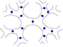
Figure 1: $D^{\star}$ and its canonical rigid structure

Definition 1.5.

Let $\varphi$ be a homeomorphism of $D^{\star}$. One says that $\varphi$ is asymptotically rigid if the following conditions are fulfilled:

• There exists an admissible subsurface $\Sigma\subset D^{\star}$ such that $\varphi(\Sigma)$ is also admissible.

• The complement $D^{\star}-\Sigma$ is an union of $n$ infinite surfaces. Then the restriction $\varphi:D^{\star}-\Sigma\to D^{\star}-\varphi(\Sigma)$ is rigid, meaning that it respects the rigid structures in the complementary of the compact subsurfaces, it maps the hexagons into hexagons. Such a surface $\Sigma$ is called a support for $\varphi$.

One denotes by $T^{\star}$ the group of asymptotically rigid homeomorphisms of $D^{\star}$ modulo isotopy through homeomorphisms which pointwise preserve the boundary $D^{\star}$.

Remark 1.4.

There exists a cyclic order on the frontier arcs of an admissible subsurface induced by the planarity. An asymptotically rigid homeomorphism necessarily preserves the cyclic order of the frontier for any admissible subsurface. In particular one can identify $T$ with the group of asymptotically rigid homeomorphisms (mod isotopy) of the ribbon tree $D$. Further $T^{\star}$ is the analogue of $T$ for the punctured disk.

1.3 Preliminaries on combings

We will follow below the terminology introduced by Bridson in [5, 6], in particular we allow very general combings. We refer the reader to [13] for a thorough introduction to the subject.

Let $G$ be a finitely generated group with a finite generating set $S$, such that $S$ is closed with respect to the inverse and corresponding Cayley graph $C(G,S)$. This graph is endowed with the word metric in which the distance $d(g,g^{\prime})$ between the vertices associated to the elements $g$ and $g^{\prime}$ of $G$ is the minimal length of a word in the generators $S$ representing the element $g^{-1}g^{\prime}$ of $G$.

A combing of the group $G$ with generating set $S$ is a map which associates to any element $g\in G$ a path $\sigma_{g}$ in the Cayley graph associated to $S$ from $1$ to $g$. In other words $\sigma_{g}$ is a word in the free group generated by $S$ that represents the element $g$ in $G$. We can also represent $\sigma_{g}(t)$ as a combing path in $C(G,S)$ that joins the identity element to $g$, moving at each step to a neighboring vertex and which becomes eventually stationary at $g$. Denote by $|\sigma_{g}|$ the length of the path $\sigma_{g}$ i.e. the smallest $t$ for which $\sigma_{g}(t)$ becomes stationary.

Definition 1.6.

The combing $\sigma$ of the group $G$ is synchronously bounded if it satisfies the synchronous fellow traveler property below. This means that there exists $K$ such that the combing paths $\sigma_{g}$ and $\sigma_{g^{\prime}}$ of two elements $g$, $g^{\prime}$ at distance $d(g,g^{\prime})=1$ are at most distance $K$ far apart at each step i.e.

$$d(\sigma_{g}(t),\sigma_{g^{\prime}}(t))\leq K,\;{\rm for\;any}\;t\in R_{+}$$

A group $G$ having an asynchronously bounded combing is asynchronously combable.

In particular, combings furnish normal forms for group elements. The existence of combings with special properties (like the fellow traveler property) has important consequences for the geometry of the group (see [1, 5]).

We will introduce also a slightly weaker condition (after Bridson and Gersten) as follows:

Definition 1.7.

The combing $\sigma$ of the group $G$ is asynchronously bounded if it satisfies the asynchronous fellow traveler property below. This means that there exists $K$ such that for any two elements $g$, $g^{\prime}$ at distance $d(g,g^{\prime})=1$ there exist ways to travel through the combing paths $\sigma_{g}$ and $\sigma_{g^{\prime}}$ at possibly different speeds so that corresponding points are at most distance $K$ far apart. Thus, there exists continuous increasing functions $\varphi(t)$ and $\varphi^{\prime}(t)$ going from zero to infinity such that

$$d(\sigma_{g}(\varphi(t)),\sigma_{g^{\prime}}(\varphi^{\prime}(t)))\leq K,\;{\rm for\;any}\;t\in R_{+}$$

The asynchronously bounded combing $\sigma$ has a departure function $D:{\mathbb{R}}_{+}\to{\mathbb{R}}_{+}$ if, for all $r>0$, $g\in G$ and $0\leq s,t\leq|\sigma_{g}|$, the assumption $|s-t|>D(r)$ implies that $d(\sigma_{g}(s),\sigma_{g}(t))>r$.

Remark 1.5.

There are known examples of asynchronously combable groups with a departure function: asynchronously automatic groups (see [13]), the fundamental group of a Haken 3-manifold ([5]), or of a geometric 3-manifold ([6]), semi-direct products of ${\mathbb{Z}}^{n}$ by ${\mathbb{Z}}$ ([5]). Gersten ([17]) proved that such groups are of type ${\rm FP}_{3}$ and announced that they should actually be ${\rm FP}_{\infty}$. Notice that there exist asynchronously combable groups (with departure function) which are not asynchronously automatic, for instance the Sol and Nil geometry groups of closed 3-manifolds (see [4]); in particular, they are not automatic.

2 The Thompson group $T$ is asynchronously combable

2.1 The group $T$ as a mapping class group

We consider the following elements of $T$, defined as mapping classes of asymptotically rigid homeomorphisms:

• The support of the element $\beta$ is the central hexagon. Further $\beta$ acts as the counterclockwise rotation of order three whose axis is vertical and which permutes the three branches of the ribbon tree issued from the hexagon.

  

• The support of $\alpha$ is the union of two adjacent hexagons, one of them being the support of $\beta$. Then $\alpha$ rotates counterclockwise the support of angle $\frac{\pi}{2}$, by permuting the four branches of the ribbon tree issued from the support.

  

Lochak and Schneps ([27]) proved that the group $T$ has the following presentation with generators $\alpha$ and $\beta$ and relations

$$\alpha^{4}=\beta^{3}=1$$

$$[\beta\alpha\beta,\alpha^{2}\beta\alpha\beta\alpha^{2}]=1$$

$$[\beta\alpha\beta,\alpha^{2}\beta^{2}\alpha^{2}\beta\alpha\beta\alpha^{2}\beta\alpha^{2}]=1$$

$$(\beta\alpha)^{5}=1$$

Remark 2.1.

If we set $A=\beta\alpha^{2}$, $B=\beta^{2}\alpha$ and $C=\beta^{2}$ then we obtain the generators $A,B,C$ of the group $T$, considered in [10]. Then the first two relations above are equivalent to

$$[AB^{-1},A^{-1}BA]=1,\,\;\;[AB^{-1},A^{-2}BA^{2}]=1$$

The presentation of $T$ in terms of the generators $A,B,C$ consists of the two relations above with four more relations to be added:

$$C^{3}=1,\;\,C=BA^{-1}CB,\,\;CA=(A^{-1}CB)^{2},\,\;(A^{-1}CB)(A^{-1}BA)=B(A^{-2}CB^{2})$$

2.2 The Ptolemy groupoid and $T$

The previous results from [16] come from the interpretation of the group $T$ (and its braided version $T^{*}$) as a mapping class group of an infinite surface. In this sequel we will bring forth another perspective, by turning back to Penner’s original approach ([30, 31]) of the Ptolemy groupoid acting on triangulations of surfaces. In the case when the surface is the hyperbolic plane $H^{2}$ Penner obtained what he called the universal Ptolemy groupoid. It was remarked that this groupoid is actually a group since all elements have inverses. A result of Kontsevich and Imbert ([24]) identified the Ptolemy groupoid with both the group $T$ and $PPSL(2,{\mathbb{Z}})$, as well. An explicit and convenient description of this isomorphism was described by Lochak and Schneps in [27], and that permitted them to obtain a nice geometric-oriented presentation of $T$.

Let us recall a few definitions which will be needed in the sequel. Details may be found in [30, 31]. One considers ideal triangulations of the hyperbolic plane $H^{2}$ having vertices at the rational points of the boundary circle and coinciding with the Farey tessellation for all but finitely many triangles. Moreover, each triangulation is labeled, by choosing a distinguished oriented edge $e$ (called the d.o.e.). This theory has been considered for arbitrary surfaces in [31].

Let $\gamma$ be an edge (i.e. an ideal arc) of the triangulation $\tau$ (unlabeled for the moment). Then $\gamma$ is a diagonal of a unique quadrilateral $Q\subset\tau$. Let $\gamma^{*}$ be the other diagonal of $Q$. The triangulation $\left(\tau-\{\gamma\}\right)\cup\{\gamma^{*}\}$, obtained from $\tau$ by removing $\gamma$ and replacing it by $\gamma^{*}$ is said to be the result of applying the flip on the edge $\gamma$. We denote by $F_{\gamma}$ this flip. The definition extends to the labeled case without modifications when $\gamma$ is not the d.o.e., by keeping the same d.o.e. When $\gamma$ is the d.o.e. we give the flipped triangulation the d.o.e. $\gamma^{*}$ with that orientation which makes the frame $\{\gamma,\gamma^{*}\}$ (in this order) positively oriented.

Flips can be composed and they form a (free) groupoid. Moreover, one assumes that two compositions are identical if their actions on a fixed triangulation are identical. One obtains a quotient groupoid, which is called the Ptolemy groupoid $PT$, and one verifies easily that all elements have inverses and thus this is actually a group. The group $PT$ is therefore generated by all possible flips on edges of the triangulation. Notice that there are infinitely many different flips on the infinite triangulation. However, one can infer from [24, 27] that the Ptolemy group $PT$ is just another instance of our familiar Thompson group $T$ (or the group of piecewise projective transformations $PPSL(2,{\mathbb{Z}})$). In particular, $PT$ is finitely presented.

Let us explain now some details concerning the identification of the Ptolemy groupoid appearing in Lochak-Schneps picture with that considered by the present authors (see also in [15, 26]). Lochak and Schneps defined two generators of $PT$, which are the two local moves below:

• The fundamental flip, which is the flip $F=F_{e}$ on the d.o.e. $e$.

• The rotation $R$ which preserves the triangulation but moves the given d.o.e. $e$ in the clockwise direction to the next edge (adjacent to $e$) of the triangle sitting on the left of the d.o.e. and containing the d.o.e. as an edge.

We wish to emphasize that these two moves are local. All other edges of the triangulation are kept pointwise fixed. It is not so difficult to show that the two local moves above generate the group $PT$, because an arbitrary flip can be obtained by conjugating the fundamental flip $F$ by a composition of rotations $R$ and orientation-reversals $F^{2}$ of the d.o.e.

There exists another way to look at the group $PT$, which makes the identification with $T$ manifest. An element of $PT$ is specified by a couple of two labeled triangulations $(\Delta,\Delta^{\prime})$ as above. We associate a homeomorphism of the closed disk $\overline{H^{2}}$ obtained by compactifying the open disk model of the hyperbolic plane, which is subject to the following requirements:

• The homeomorphism is piecewise linear with respect to the triangulations $\Delta$ and $\Delta^{\prime}$. This means that it sends each triangle of $\Delta$ onto some triangle of $\Delta^{\prime}$ by a transformation from $PSL(2,{\mathbb{Z}})$.

• The homeomorphism sends the d.o.e. of $\Delta$ onto the d.o.e. of $\Delta^{\prime}$ with the corresponding orientation.

The homeomorphism is then uniquely determined by the two conditions above and it is an element of $PPSL(2,{\mathbb{Z}})$. It is also determined by its restriction to the boundary, when $PPSL(2,{\mathbb{Z}})$ is viewed as a subgroup of ${\rm Homeo}_{+}(S^{1})$. Denote by $\Phi:PPSL(2,{\mathbb{Z}})\to PT$ the inverse correspondence. Recall that $PPSL(2,{\mathbb{Z}})$ is isomorphic to the group $T$. For instance we identify a mapping class defined by an element $x$ of $T$ from the previous section with the element of $PPSL(2,{\mathbb{Z}})$ that has the same action as $x$ on the triangulation of $H^{2}$ in which boundary circles of $D$ are crushed onto the vertices of the Farey triangulation. Using this identification between $T$ and $PPSL(2,{\mathbb{Z}})$ we can state:

Lemma 2.2.

The map $\Phi$ is the unique anti-isomorphism between $T$ and $PT$ determined by the formulas:

$$\Phi(\alpha)=F,\;\;\Phi(\beta)=R$$

where $\alpha,\beta$ are the generators of $T$ from the previous section.

Proof.

The local moves can act far way by means of conjugacies. One associates to the local move $x$ the element $\Phi(x)\in T$. If we want to compute the action of $\Phi(\gamma\cdot x)$ we compute first the action of $\Phi(x)$ and then we have to act by some transformation $\Lambda$ which has the same effect as $\Phi(\gamma)$ had on the initial triangulation. But the triangulation has been changed by means of $\Phi(x)$. This means that the transformation $\Lambda$ is therefore equal to $\Phi(x)\Phi(\gamma)\Phi(x^{-1})$. This implies that $\Phi(\gamma\cdot x)=\Phi(x)\Phi(\gamma)\Phi(x^{-1})\Phi(x)=\Phi(x)\Phi(\gamma)$. ∎

Remark 2.3.

This correspondence will be essential below. It enables us to express arbitrary flips on a triangulation in terms of the local moves $F$ and $R$. Since the moves are local, small words will lead to small differences in the triangulations. Eventually, we can translate (by means of the canonical anti-isomorphism which reverse the order of letters in a word) any word in the generators $R$ and $F$ into an element of the group $T$, viewed as a word in the standard generators $\alpha$ and $\beta$. It is more difficult to understand the properties of a combing in terms of the action of $\alpha$ and $\beta$ on triangulations since the action is not local, and thus a short word might have a quite large effect on the combinatorics of the triangulation.

2.3 Mosher’s normal form for elements of $T$ on infinitely many flips

Mosher proved that mapping class groups of finite surfaces are automatic ([29]). One might expect then that mapping class groups of infinite surfaces share also some properties closed to the automaticity, but suitably weakened by the infiniteness assumption.

The aim of this section is to define a first natural combing for $T$ derived from Mosher’s normal form. Unfortunately, this combing is unbounded. We will show next that it can be modified so that the new combing is asynchronously bounded.

Mosher’s proof of automaticity consists of embedding the mapping class group in the corresponding Ptolemy groupoid and derive normal forms (leading to combings) for the latter. The way to derive normal forms is however valid for all kind of surfaces, without restriction of their – possibly infinite – topology. The alphabet used by the automatic structure is based on the set of combinatorial types of flips. The only point where the finiteness was used by Mosher is when one observes that the number of different combinatorial flips on a triangulated surface (with fixed number of vertices) is finite, provided that the surface is finite. Thus, the same proof does not apply to the case of $T$, since there are infinitely many combinatorially distinct flips. Nevertheless, we already remarked that we can express an arbitrary flip on the infinite triangulation as a composition of the two elements $F$ and $R$. This observation will enable us to rewrite the Mosher combing in the Ptolemy group (which uses all flips as generators) as a new combing which uses only the two generators $F$ and $R$. We will call it the Mosher-type combing of $T$. Recall that it is equivalent to a combing in our favorite generators $\alpha$ and $\beta$.

Let us recall the normal forms for elements of $T$, in terms of flips. Choose a base triangulation $\tau_{B}$, fixed once for all, for instance the Farey triangulation. Choose a total ordering on the edges of the triangulation $\tau_{B}$, say $e_{1},e_{2},e_{3},\ldots$, so that $e_{1}=e$ is the d.o.e., and choose an arbitrary orientation on each edge. The combing might depend on the particular choice we made. Given an element $\zeta\in PT$ we represent it as the couple of labeled triangulations $(\tau_{B},\tau)$. These two triangulation are identical outside some finite polygon, on which the restriction of the two triangulations are different. Let us denote by $\tau_{B}^{f}$ and $\tau^{f}$ the restrictions of the two triangulations to the finite polygon. Then $\tau^{f}$ is obtained from $\tau_{B}^{f}$ by removing several disjoint edges, say $g_{1}=e_{j_{1}}<g_{2}=e_{j_{2}}<\ldots<g_{k}=e_{j_{k}}$, from $\tau_{B}$ and replacing them by another $k$ disjoint ideal arcs (which do not belong to $\tau_{B}$) having the same set of endpoints.

As it is well-known any two triangulations of a polygon could be obtained one from another by means of several flips. Moreover, if the polygon had $n$ vertices and thus it is partitioned into $(n-2)$ triangles then the minimal number of flips needed to transform one triangulation into another one is $2n-10$, and this estimation is sharp for large $n$, as it was proved by Sleator, Tarjan and Thurston (see [33]). Notice that in our case the size of the polygon is not a priori bounded since there exist elements of $T$ whose support might be arbitrarily large.

Further we construct a series of flips followed by a relabeling move, the sequence being uniquely determined by the given element $(\tau_{B},\tau)$. The edges $g_{1},g_{2},\ldots,g_{k}$ are called the uncombed edges (in this order). Consider the first one, namely $g_{1}$. We define a prong of a triangulation to be a germ of the angle determined by two edges of the triangulation which are incident, thus having a common vertex. We say that an oriented ideal arc $g$ belongs to some prong of the triangulation $\tau^{f}$ if the start point of $g$ is the vertex of the prong and $g$ is locally contained in the prong.

Start with $g=g_{1}$ and recall that $g$ has been given an orientation. Pick up the unique prong of $\tau^{f}$ to which $g$ belongs. This prong is determined by the two edges $f^{L}$ and $f^{R}$, sitting on the left and respectively on the right of $g$. Therefore there exists another edge - say $f^{*}$ - of $\tau^{f}$ joining the two endpoints of $f^{L}$ and $f^{R}$, other than the vertex of the prong and forming a triangle $T$ with the prong edges. Further there exists another triangle $T^{*}$ of $\tau^{f}$ which shares the edge $f^{*}$ with $T$, but whose interior is disjoint from $T$, and thus it lies in the opposite half-plane determined by $f^{*}$. It is clear that $g$ intersects $f^{*}$ in one point.

The first step in combing is to use the flip on the edge $f^{*}$, which replaces $f^{*}$ by the other diagonal $f^{**}$ in the quadrilateral $T\cup T^{*}$. If $g$ was precisely the diagonal $f^{**}$ of $T\cup T^{*}$ then we succeeded in combing it, since it will belong to the new triangulation $\tau_{1}$, obtained by flipping. We will restart our procedure for $g=g_{2}$ and so on. Otherwise, it means that $g$ is still uncombed in the new triangulation. The former prong determined by the arcs $f^{L}$ and $f^{R}$ is now split into the union of two prongs because we added one more arc, namely $f^{**}$ which shares the same vertex. Then $g$ will belong to precisely one of the two new prongs, either to that determined by $f^{L}$ and $f^{**}$, or to that determined by $f^{R}$ and $f^{**}$. We change the notations for the arcs of the new prong to which $g$ belongs so that the edge of the left is $f_{2}^{L}$ and the edge of the right is $f_{2}^{R}$. Then we restart the algorithm used above for $f_{1}=f$. Namely, consider the triangle $T_{2}$ determined by the two edges $f_{2}^{L}$ and $f_{2}^{R}$ and the edge $f_{2}^{*}$ connecting their endpoints, and next the opposite triangle $T_{2}^{*}$. Use the flip on the edge $f_{2}^{*}$, and continue this way.

The lemma Combing terminates section 2.5 of [29] tells us that after finitely many steps we obtain a triangulation for which $g_{1}$ is combed. We continue then by using the same procedure in combing $g_{2}$ and then $g_{3}$ and so on, until all $g_{j}$ (for $j\leq k$) are combed. At the end we need to relabel the d.o.e. in order to bring it to the d.o.e. of $\tau_{B}$. The sequence of flips and corresponding triangulations $\tau\to\tau_{1}\to\tau_{2}\to\cdots\tau_{N}\to\tau_{B}\to\tau_{B}$ (the last move being a relabelling) is called the Mosher normal form of the element $\zeta$ of $T$.

As already mentioned before this normal form is not convenient for us as it states, since there are infinitely many distinct combinatorial flips. We can overcome this difficulty by translating in the simplest possible way Mosher’s normal form into a word in $F$ and $R$. In this case the flip $F$ cannot be applied but on the d.o.e. We assume that the d.o.e. $e_{\tau}$ of $\tau$ belongs to the polygon associated to $\tau_{f}$ and the same for $\tau_{B}$. This can be realized by enlarging the size of the support.

In order to apply a flip to the triangulation $\tau_{f}$ we notice that we have first to move the d.o.e. from its initial position onto the edge which we want to be flipped. Let us assume for the moment that it is always possible to do this in a canonical way. Let $\tau$ be an arbitrary unlabeled triangulation (finite or not) and $e,f$ two oriented edges. We define the transfer $T_{e,f}(\tau)$ as being the (unique) element of $T$ which sends the labeled triangulation $(\tau,e)$ into the labeled triangulation $(\tau,f)$.

The normal form obtained above for $\zeta$ can be read now in the following way:

1. Locate the first edge to be flipped, namely $f_{1}^{*}$, of $\tau^{f}$. Use the transfer $T_{e_{\tau},f_{1}^{*}}(\tau^{f})$ in order to move the d.o.e. from $e_{\tau}$ to $f_{1}^{*}$.

2. Use the flip $F$, which will be located at $f_{1}^{*}$ and thus it will act exactly as the flip considered in the Mosher normal form.

3. The new d.o.e. is the image $F(f_{1}^{*})$ of the former d.o.e. with the d.o.e. orientation induced by the flip. Locate the new edge to be flipped, say $f_{2}^{*}$. Use the transfer $T_{f_{1}^{*},f_{2}^{*}}(F_{f_{1}^{*}}(\tau^{f}))$.

4. Continue until all uncombed edges are combed.

5. If all edges were combed, then use eventually the transfer $T_{f_{N}^{*},e}(F_{f_{N}^{*}}(\cdots(F_{f_{1}^{*}}(\tau^{f}))\cdots)$ in order to bring the d.o.e. at its right place.

2.4 Writing Mosher’s normal form as two-generator words

We will explain now how any transfer can be written canonically as a word in the two letters $F$ and $R$, corresponding to the respective generators of $T$. This procedure will be called then the translation of Mosher’s normal form. In fact, the transfer moves preserve the combinatorics of the triangulation, and thus they can be identified (by means of the anti-isomorphism $\Phi^{-1}$ encountered above) with automorphisms of the dual tree. Using this identification each transfer $T_{e,f}(\tau)$ corresponds to the element of the modular group $PSL(2,{\mathbb{Z}})$ whose action on the binary tree sends the edge dual to $e$ to the edge dual to $f$. Now, it is well-known that $PSL(2,{\mathbb{Z}})$ has an automatic structure and thus any element can be given a normal form in the standard generators. However, one can do this in an explicit elementary way. In fact the subgroup $PSL(2,{\mathbb{Z}})$ of $T$ is actually the (sub)group generated by the elements $\alpha^{2}$ and $\beta$. Furthermore, since we have $PSL(2,{\mathbb{Z}})={\mathbb{Z}}/2{\mathbb{Z}}*{\mathbb{Z}}/3{\mathbb{Z}}$, it follows that any element of $PSL(2,{\mathbb{Z}})$ can be uniquely written as a word

$$\beta^{\epsilon_{0}}\alpha^{2}\beta^{\epsilon_{1}}\alpha^{2}\cdots\alpha^{2}\beta^{\epsilon_{m+1}},\;\;{\rm where}\,\;\epsilon_{0},\epsilon_{m+1}\in\{0,1,2\}\;\,{\rm and}\;\;\epsilon_{1},\epsilon_{2},\ldots,\epsilon_{m}\in\{1,2\}$$

Moreover, the factors $\epsilon_{j}$ can be effectively computed. There exist a completely analogous description in terms of the triangulations and the moves $F^{2}$ and $R$. We will explain this in the dual setting (since anyway the final result can be easily recorded as a word in $\alpha$ and $\beta)$. The ideal arcs $e$ and $f$ correspond to the edges of the dual binary tree ${\rm Tree}(\tau)$ of the triangulation $\tau$. Recall that all edges of $\tau$ have been given an orientation. This induces a co-orientation of the edges of ${\rm Tree}(\tau)$, namely a unit vector orthogonal to each edge of ${\rm Tree}(\tau)$. One might choose a natural co-orientation for ${\rm Tree}(\tau)$ by asking it to turn clockwisely in the standard planar embedding of the binary tree, in which case the formulas are simpler. However, it would be preferable to do the computations in the general situation. Moreover, ${\rm Tree}(\tau)$ is a rooted tree, whose root is the vertex of ${\rm Tree}(\tau)$ sitting in the right of the edge dual to the d.o.e. $e_{\tau}=e$. In order to fix it we used the co-orientation. Moreover, for any edge $g$ of the tree and chosen vertex $v$ of $g$ it makes sense to speak about the two other edges incident to $g$ at $v$, which are: one at the left of $g$ and the other one at the right of $g$. This follows from the natural circular order around each vertex inherited from the embedding of the dual tree in the plane. If $e$ and $f$ are – not necessarily distinct – edges incident at some vertex, we set:

$$\epsilon(e,f)=\left\{\begin{array}[]{ll}0&{\rm if}\;e=f\\ 1&{\rm if}\;f\;{\rm is\;on\;the\;left\;of}\;e\\ 2&{\rm otherwise}\end{array}\right.$$

Furthermore, if we identify $\alpha^{2}$ and $\beta$ with elements of $PSL(2,{\mathbb{Z}})$ which act as planar tree automorphisms, it makes sense to look at the image of the co-orientation of an edge $e$ by means of the element $\xi\in PSL(2,{\mathbb{Z}})$. For instance $\alpha^{2}$ reverts the orientation of the d.o.e.

Let then $\gamma=(h_{1},h_{2},\ldots,h_{q})$ be the unique geodesic in ${\rm Tree}(\tau)$ which joins the root (which is an endpoint of $e$) to $f$. It might happen that either $h_{1}=e$ or $h_{1}\neq e$, but in any case we have always $h_{q}\neq f$. We claim now that:

$$\Phi^{-1}(T_{e,f}(\tau))=\beta^{\epsilon_{0}}\alpha^{2}\beta^{\epsilon_{1}}\alpha^{2}\cdots\beta^{\epsilon_{q}}\alpha^{2\delta}$$

where

$$\epsilon_{0}=\epsilon(e,h_{1}),\;\epsilon_{1}=\epsilon(h_{1},h_{2}),\ldots\epsilon_{q}=\epsilon(h_{q},f)$$

and

$$\delta=\left\{\begin{array}[]{ll}0&{\rm if}\;f\;\mbox{has the co-orientation induced from }e\\ 1&{\rm otherwise}\end{array}\right.$$

Remark that the intermediary co-orientations of $h_{j}$ do not influence the normal form.

Remark 2.4.

If the triangulated subpolygon of the Farey triangulation is connected then it is actually a convex polygon in the plane. In particular, if $e,f$ are edges of some of its triangulations and $h_{j}$ are edges dual to a geodesic joining the two dual edges, then all $h_{j}$ are contained in the respective subpolygon. Thus, in the process of of combing uncombed edges we can realize all flips and transfers within the given, fixed polygon.

Definition 2.1.

The Mosher-type combing (or normal form) for elements of $T$ is defined as follows. For each $\zeta=(\tau_{B},\tau)\in T$ we choose the restricted triangulations $\tau_{B}^{f},\tau^{f}$ so that the associated polygon is the smallest connected polygon containing all uncombed arcs of $\tau$ and both d.o.e.’s. Notice that this is uniquely determined. The normal form of $\zeta\in T$ is then the sequence

$$\sigma^{M}_{\zeta}=[T_{e_{\tau},f_{1}^{*}}(\tau^{f}),\;F,\;T_{f_{1}^{*},f_{2}^{*}}(F_{f_{1}^{*}}(\tau)),\;F,\;\ldots\;,\;F,\;T_{f_{N}^{*},e}(F_{f_{N}^{*}}(\cdots(F_{f_{1}^{*}}(\tau^{f}))\cdots)]$$

in which each transfer is translated as a canonical word in $R$ and $F$. We might eventually use $\Phi$ in order to uncover the word in $\alpha$ and $\beta$.

Recall that Mosher’s combing of the mapping class group is asynchronously bounded in the case when the surface is finite. This follows from the fact that, given two elements $\zeta,\widetilde{\zeta}$ at distance one in the Cayley graph of the respective Ptolemy groupoid, then one can write

$$\sigma^{M}_{\zeta}=w_{0}z_{1}w_{1}z_{2}w_{2}\cdots z_{p}w_{p},\;\;\sigma^{M}_{\widetilde{\zeta}}=\widetilde{w_{0}}z_{1}\widetilde{w_{1}}z_{2}\widetilde{w_{2}}\cdots z_{p}\widetilde{w_{p}}$$

where $z_{i},w_{i}$ are words in the generators, such that:

1. First, the size of the subwords on which the combings don’t agree are uniformly bounded:

   $$|w_{i}|,|\widetilde{w_{i}}|\leq K,\;\;{\rm for\;all}\;\;i\leq p$$

2. Second, for all $m$, the distance between the corresponding prefix elements which are represented by the prefix words $\sigma^{M}_{\zeta}(m)=w_{0}z_{1}w_{1}z_{2}w_{2}\cdots z_{m}$ and $\sigma^{M}_{\widetilde{\zeta}}(m)=\widetilde{w_{0}}z_{1}\widetilde{w_{1}}z_{2}\widetilde{w_{2}}\cdots z_{m}$ is uniformly bounded, when these elements are considered in the Cayley graph of the Ptolemy groupoid. Actually, the two prefix elements are always at distance one, because they differ by precisely one flip.

Let us analyze what happens in the infinite case, when the Ptolemy group is $T$. We rewrite the combing in the two-generator free group and thus we have to rewrite also the flip relying the two prefix elements above. Since there are flips which are arbitrarily far away, we will need arbitrary long words in $R$ and $F$, and thus the Mosher-type combing is not asynchronously bounded. Notice however, that the first part of the assertion above is still true in this case. This follows from the fact that $\zeta,\widetilde{\zeta}$ are at distance one in the two-generator Cayley graph if they differ by a fundamental flip or by a rotation move $R$. In the second case the combing paths are the same except for the first few moves which realize the first transfer.

2.5 Modifying the Mosher-type combing in order to get asynchronous boundedness

We turn back to the original description of the Mosher combing of $T$ in terms of the infinitely many flips of the triangulation. Any element $\zeta=(\tau_{B},\tau)$ of $T$ was brought to its normal form

$$F_{e_{1}},F_{e_{2}},\ldots,F_{e_{N}},P$$

where $F_{e_{i}}$ are flips and $P$ is the last relabelling move. We will first define the new combing – denoted $\sigma$ – in the usual generators $R$ and $F$ for each flip $F_{e}$ and then concatenate the combings according to the pattern of the Mosher normal form above. Recall that the Mosher-type combing defined above for the flip $F_{f}$ was the simplest possible (actually geodesic): we used the transfer of the d.o.e. $e$ to $f$, further the fundamental flip $F$, and then we transfered the d.o.e. $F(f)$ back to its initial position $e$. This time we will be more careful about the way we will achieve the flip $F_{f}$.

Consider the element $\widetilde{\zeta}$ of $T$ at distance $1$ from $\zeta$. Let us assume that $\widetilde{\zeta}=F\zeta$. Then $\widetilde{\zeta}=(\tau_{B},\widetilde{\tau})$, where $\widetilde{\tau}=F\tau$ is the triangulation with the d.o.e. $F(e)=e^{*}$.

The failure of the boundedness for the Mosher-type combing above is a consequence of the fact that the distance between $T_{e,f}(\tau)$ and $T_{e^{*},f}(\widetilde{\tau})$ grows linearly with the distance $d(e,f)$ between the edges $e$ and $f$.

We want to define a path $P(\tau,F_{f}(\tau))$ joining $\tau$ to $F_{f}(\tau)$ such that the asynchronous distance between the paths $P(\tau,F_{f}(\tau))$ and $P(\widetilde{\tau},F_{f}(\widetilde{\tau}))$ is uniformly bounded, independently on the position of $f$.

Let us denote by $Q_{f}$ the quadrilateral determined by the edge $f$, which has $f$ and $f^{*}$ as diagonals. We have two distinct cases to analyze: either $f$ is disjoint from $Q_{e}$ or $f$ belongs to $Q_{e}$.

(1.) Assume that $f$ is disjoint from $Q=Q_{e}$. Consider the chain of triangles joining $e$ to $f$, which is dual of the geodesic joining $e$ to $f$ in the dual tree. Denote their union by $Z(e,f)\subset\tau$.

Lemma 2.5.

There exists a sequence of labeled triangulations $\tau_{n}$ with d.o.e. $e_{n}$ and a sequence of polygons $Z_{n}\subset Z(e,f)$ such that

1. For all $n$ we have $e_{n},e_{n+1}\in Z_{n}$;

2. We have $Q\subset Z_{n}$ for all $n$;

3. The number of vertices of $Z_{n}$ is uniformly bounded by $K$. We will see that $K=7$ suffices;

4. For $n$ large enough $Z_{n}=Q\cup W_{n}$, where $W_{n}$ and $Q_{f}$ have a common edge.

Proof.

Consider thus the triangulated polygon $A=Z(e,f)-Q\cup Q_{f}$, which can be seen as a chain of triangles joining the edges $e^{\prime}\in Q$ (adjacent to $e$) and $f^{\prime}\in Q_{f}$ (adjacent to $f$). This chain of triangles is dual to a geodesic in the binary dual tree and thus it contains the minimal number of possible triangles. This polygon is embedded in the plane and it makes sense to speak about the left vertex $a_{1}$ of $e^{\prime}$ and the right vertex $b_{1}$ of $e^{\prime}$. If we start traveling in the clockwise direction along the boundary of $A$ and starting at $a_{1}$ then we will encounter, in this order, the vertices $a_{2},...,a_{s}$, the last one being a vertex of $f^{\prime}$. Further if we travel in the counterclockwise direction from $b_{1}$ we will encounter the vertices $b_{2},b_{3},\ldots,b_{t}$, the last point being the other vertex of $f^{\prime}$. If $s,t\leq 2$ then there is nothing to prove. Assume that $t\geq 3$, the other case being symmetric. Consider the points $b_{1},b_{2},b_{3}$ and the smallest triangulated subpolygon $B\subset A$ containing these three vertices. It is understood that the triangulation of $B$ is the restriction of that from $A$ and the adjective smallest means that it contains the minimum number of triangles. Notice that edges of the triangulation of $A$ cannot join two vertices on the same side, since otherwise the subpolygon they would determine (part of the boundary and this edge) could be removed from $A$, thus contradicting the minimality of the chain $A$.

Assume that $B$ has the vertices $a_{1},a_{2},...,a_{m}$ from the left side and $b_{1},b_{2},b_{3}$ from the right side.

If $m\geq 3$ then there exists a subpolygon $W_{1}$ containing $a_{1}b_{1}$ of height at most 3. This means a subpolygon containing three consecutive points on the same side, say $b_{1},b_{2},b_{3}$, and at most two vertices consecutive vertices on the other side say $a_{1},a_{2}$. If $m\leq 2$ this is obvious. Suppose now that $m\geq 3$.

Since $B$ has $m+3$ vertices one needs $m$ diagonals in order to triangulate $B$. Let us denote by $m_{j}$ the number of diagonals having $b_{j}$ as endpoint. We have then $m_{1}+m_{2}+m_{3}=m$. If $m_{1}\geq 2$ then the diagonals exiting $b_{1}$ should arrive at $a_{2},a_{3}$ and thus the quadrilateral $a_{1}a_{2}a_{3}b_{1}$ has the claimed property. Suppose $m_{1}=1$; if $m_{2}=1$ then the diagonals are $a_{2}b_{1},a_{2}b_{2},a_{3}b_{2}$ and the subpolygon is $a_{1}a_{2}a_{3}b_{2}b_{1}$. If $m_{2}=1$ then $m_{3}\geq 1$ and thus there exists the diagonal $a_{2}b_{3}$ and thus the subpolygon $a_{1}a_{2}b_{3}b_{2}b_{1}$ verifies the claim.

Consider next the polygon $Z_{1}=Q\cup W_{1}$. Remark that $Z_{1}$ has at most 7 vertices. We can use flips and transfers inside $Z_{1}$ (notice that the d.o.e. lays within $Q\subset Z_{1}$) in order to change the triangulation so that the tree consecutive points on one side of $W_{1}$ form now a triangle. We suppose that the d.o.e. is brought back into its position.

Denote by $\tau_{2}$ the new triangulation. The chain of triangles $Z_{2}(e,f)$ which joins $e$ to $f$ within $\tau_{2}$ has one triangle less, because we can exclude the triangle $b_{1}b_{2}b_{3}$; actually one of the paths $a_{1},a_{2},\ldots,a_{s}$ or $b_{1},b_{2},\ldots,b_{s}$ becomes one unit shorter.

Continue the same procedure with the the polygon $A_{2}=Z_{2}(e,f)-Q\cup Q_{f}$, and define inductively the polygons $W_{2}$, $Z_{2}=Q\cup W_{2}$ and so on, until we obtain a polygon $W_{N}$ that contains both $a_{1}b_{1}$ and $a_{s}b_{t}$. This proves the claim. ∎

Let us define now the combing of the flip $F_{f}$, as follows. The lemma 2.5 shows that that there exist the subpolygons $Z_{n}$ constructed as above so that eventually $Z_{n}=Q\cup W_{n}$ where $W_{n}$ and $Q_{f}$ have a common edge. We will use the sequence $Z_{j}$ in order to join the d.o.e. $e$ to $f$. However instead of going straight away from $e$ to $f$ along the shortest path we will consider the sequence $\tau_{n}$ of triangulations that makes eventually the edges $e$ and $f$ to become close to each other. At each step, we consider only those flips or rotations which can be realized inside the respective $Z_{j}$ and that changes $\tau_{j}$ into $\tau_{j+1}$. Finally we obtain a triangulation containing $Z_{n}$. We will say that we modified the triangulation in order to make the transfer $T_{e,f}$ short. Now, the polygon $Z_{n}\cup Q_{f}$ contains both $Q$ and $Q_{f}$ and has at most 9 vertices. Therefore we can realize the flip $F_{f}$ within $Z_{n}\cup Q_{f}$, by using the transfer $T_{e,f}$ within the 9-vertices polygon, followed by the fundamental flip $F$ and then by the inverse transfer $T_{e,f}^{-1}$. The effect on the triangulation was precisely that of $F_{f}$.

Next, after the flip $F_{f}$ was performed, we use the the same procedure by means of the subpolygons $Z_{n}$ and the inverse sequence of associated triangulations in order to move backwards thru triangulations and finally reconstruct the original triangulation within the polygon $Z(e,f)$, without touching anymore to $Q_{f}$. Eventually, we obtain a triangulation corresponding to $F_{f}\tau$.

Definition 2.2.

The path $P(\tau,F_{f}\tau)$ consisting of transformations (flips and rotations) between triangulations that join $\tau$ to $F_{f}\tau$ is the combing $\sigma_{F_{f}}$ of $F_{f}$.

Remark 2.6.

There is some freedom in choosing the way to transform the triangulations within each $Z_{n}$. However, this does not influence the boundedness properties of the combing. We can easily find canonical representatives, since there are finitely many choices.

Lemma 2.7.

Assume that $\widetilde{\tau}=F\tau$ differ by a flip $F$ and $f$ is an edge disjoint from $Q$. Then the combing paths $P(\tau,F_{f}\tau)$ and $P(\widetilde{\tau},F_{f}(\widetilde{\tau}))$ stay at bounded asynchronous distance in the standard two generators Cayley graph of $T$.

Proof.

We have the sequences $Z_{n},\widetilde{Z_{n}}$ as above. Then $Q_{e^{*}}=Q_{e}=Q$, and thus $Z_{n}\cap\widetilde{Z_{n}}\supset Q$ for all $n$. Further, for $n$ large enough we have $W_{n}=\widetilde{W_{n}}$ is a pentagon containing both an edge of $Q$ and an edge of $Q_{f}$.

Now, for any $n$ the polygon $Z_{n}\cup\widetilde{Z_{n}}$ is connected and has at most $8$ vertices, since both lay in the same half space determined by the common edge $e^{\prime}$ and thus have one more common vertex. This means that one can pass from $(\tau_{n},e_{n})$ to $(\widetilde{\tau_{n}},\widetilde{e_{n}})$ by using only flips and transfers taking place in the finite polygon $Z_{n}\cup\widetilde{Z_{n}}$ and thus they are at bounded distance. For instance their distance is smaller than the diameter of the graph of transformations of a 8-vertices polygon (using $F$ and $R$) which is smaller than $30$. ∎

(2.) The second case to be considered is when $f$ is a nearby edge, namely an edge of $Q$.

Definition 2.3.

If $f\in Q$ then $\sigma_{F_{f}}$ is the Mosher-type combing of $F_{f}$ in the two-generators, i.e. $\sigma^{M}_{F_{f}}$.

We are able now to define the combing of a general element of $T$. Let us consider $\zeta\in T$, which is written in Mosher’s normal form in terms of arbitrary flips as a sequence $F_{f_{1}},F_{f_{2}},...,F_{f_{N}}$ followed by a relabelling move $P$ bringing the d.o.e. at its place.

We consider that the d.o.e. is at position $e$ and we replace each flip $F_{f_{j}}$ in the sequence above by its combing $P(\tau_{j},F_{f_{j}}\tau_{j})$, where $\tau_{j+1}=F_{f_{j}}\tau_{j}$. The d.o.e. remains at the same place $e$, except when $f_{j}=e$ in which case is transformed accordingly. At the end we obtain the triangulation $\tau_{B}$ with some place for the d.o.e. which is then transferred by means of the Mosher-type combing of the transfer onto its standard location.

2.6 The combing of $T$ is asynchronously bounded

The proof follows now the same lines as Mosher’s proof. Consider $\zeta$ and $\widetilde{\zeta}$ two elements at distance one. We have either $\widetilde{\zeta}=F\zeta$ or $\widetilde{\zeta}=R\zeta$.

Proposition 2.8.

The combing defined above for $T$ is asynchronously bounded, and we can take the constant $K=30$.

Proof.

We have either $\widetilde{\zeta}=F\zeta$ or $\widetilde{\zeta}=R\zeta$. It suffices to analyze the first case, the second case being simpler and resulting by the same argument. Let us consider the Mosher normal forms

$$F_{f_{1}},F_{f_{2}},\ldots,F_{f_{n}},P~{}\;\mbox{\rm and respectively }~{}\;\widetilde{F}_{f_{1}},\widetilde{F}_{f_{2}},\ldots,\widetilde{F}_{f_{n}},\widetilde{P}$$

From [29] section 2.5 this combing is asynchronously bounded if we consider all flips as generators, and moreover the combing sequences $F_{f_{j}}$ and $\widetilde{F_{f_{j}}}$ coincide at those positions corresponding to flips outside the quadrilateral $Q$. Notice that our $F$ is located at the d.o.e. while [29] deals with the general case of the flip which can be outside the d.o.e. Therefore the idea of the proof is very simple: the points in the Mosher combing corresponding to the flips which are located at edges of $Q$ are at bounded distance from each other; this distance is measured by composing a few flips, which are themselves flips on edges uniformly closer to the d.o.e. Thus after transforming them into paths in the two generator Cayley graph these points will be only a bounded amount apart. The points corresponding to flips on edges which are far from the d.o.e. could be very far away in the Mosher-type combing, but these points come from identical sequences of flips and each flip has been combed now using the paths $P(\tau,F_{f}\tau)$. The lemma 2.5 shows that these points will remain also a finite amount apart. Eventually, we have to see what happens when using the relabelling moves $P,\widetilde{P}$. It suffices to observe that the d.o.e. of $\tau$ will remain always closed-by to the d.o.e. of $\widetilde{\tau}$, and actually in the same quadrilateral. This means that the last transfer of d.o.e. leads to two normal forms which are very closed to each other. This will prove the claim.

It suffices thus to see what happens with Mosher-type combing when we meet nearby edges to be flipped.

Let $f_{1}^{*}$ be the first edge to be flipped and $e=e_{\tau}$ be the d.o.e. We have to compare $T_{e,f_{1}^{*}}(\tau^{f})$ and $T_{\beta(e),f_{1}^{*}}(\tau^{f})$. An alternative way is to look at the dual tree. Recall that ideal arcs of the triangulation yield edges of the dual tree. We have to compare the two geodesics $\gamma$ and $\widetilde{\gamma}$ which join the left endpoints of the edges $e$ and respectively $\beta(e)$ to some endpoint of $f_{1}^{*}$. But the left endpoints of $e$ and $\beta(e)$ coincide and thus $\gamma=\widetilde{\gamma}$. Thus the transfer are given by identical words except possibly for the first three letters.

The next case is when $\widetilde{\zeta}=\alpha\zeta$. Then the differences between the normal forms can propagate to all other transfers and not just to the first one. Another difficulty is that the dual trees are different. We set ${\mathcal{T}}={\rm Tree}(\tau)$ and ${\mathcal{T}}_{t}$ for the dual tree after $t$ steps. We define a step to be the action of a block of several consecutive letters of the normal form. The precise control on the size of blocks will be given below. We set also $\widetilde{{\mathcal{T}}}={\rm Tree}(\alpha\tau)$ and then $\widetilde{{\mathcal{T}}}_{t}$ for the dual tree after $t$ steps. The steps in the two cases are not necessary correlated. Instead, we would rather want a certain correlation between the trees ${\mathcal{T}}_{t}$ and $\widetilde{{\mathcal{T}}}_{t}$, for any $t$.

The trees ${\mathcal{T}}$ and $\widetilde{{\mathcal{T}}}$ are identical except for the image of the support $\Sigma$ of the move $\alpha$, which is made of the edge $e$ and its four adjacent edges. We have $\widetilde{{\mathcal{T}}}={\mathcal{T}}-\Sigma\cup\alpha\Sigma$, where $\Sigma$ is replaced by its image by $\alpha$ (i.e. a rotation of angle $\frac{\pi}{2}$). We would like to define the steps in such a way that any moment $t$ we have $\widetilde{{\mathcal{T}}}_{t}={\mathcal{T}}_{t}-\Sigma_{t}\cup\alpha\Sigma_{t}$, where $\Sigma_{t}$ is combinatorially isomorphic to $\Sigma$. We call $\Sigma_{t}$ the singular locus at step $t$ and denote $\widetilde{\Sigma_{t}}=\alpha\Sigma_{t}$. Moreover we have a natural combinatorial isomorphism between the two trees, outside their respective singular loci. Let $e_{t}$ denotes the central edge of $\Sigma_{t}$ and $\widetilde{e_{t}}$ for $\widetilde{\Sigma_{t}}$.

In order to get control on the differences between the normal forms in the two cases we have to understand what happens if we have to use transfers or flips which touch the singular locus. In fact, any transfer between two edges lying in the same connected component of ${\mathcal{T}}_{t}-\Sigma_{t}$ has a counterpart as a transfer in $\widetilde{{\mathcal{T}}_{t}}-\widetilde{\Sigma_{t}}$ given by the same word.

As we saw previously the transfer between two edges is determined by the geodesic joining the two edges. We have then to understand what happens when such a geodesic penetrates in the singular locus. We have also to consider the case when we encounter a flip on an edge from the singular locus. There are a few cases to consider:

1. If the geodesic enters and exit the singular locus. Let $\gamma=(h_{1},h_{2},\ldots,h_{q})$, and respectively $\widetilde{\gamma}=(\widetilde{h_{1}},\widetilde{h_{2}},\ldots,\widetilde{h_{q}})$ be the two corresponding geodesics which join two edges $f$ and $g$ which are corresponding to each other and both lay outside the singular locus. It follows that $\gamma-\gamma\cap\Sigma_{t}=\widetilde{\gamma}-\widetilde{\gamma}\cap\widetilde{\Sigma_{t}}$ and the only differences can be seen at the level of the singular loci. According to the formula for the transfer we can write then

   $$T_{f,g}(\tau^{f}_{t})=z_{1}w_{1}z_{2},\;T_{f,g}(\widetilde{\tau^{f}_{t}})=z_{1}\widetilde{w_{1}}z_{2}$$

   where the words $w_{1},\widetilde{w_{1}}$ record the transformations needed to transfer one edge to another within the singular locus. The longest such word is $\alpha^{2}\beta\alpha^{2}\beta^{2}\alpha^{2}$ and thus $|w_{1}|,|\widetilde{w_{1}}|\leq 9$.

2. If the geodesic enters the singular locus and does not exit, or a geodesic starts from the singular locus and exits. This means that we have a transfer from an edge outside the singular locus to an edge of the singular locus.

   If this transfer is the final operation and the normal form is achieved for $\zeta$, then normal form of $\widetilde{\zeta}$ is obtained by flipping the edge $\widetilde{e_{t}}$.

   Otherwise we didn’t reach yet the normal form in neither of the two configurations. Thus the transfer is followed by a flip on some edge in the singular locus. We have two subcases:

   1. The flip acts on some edge $f$ of the singular locus incident but different from to $e_{t}$ in $\tau^{f}$ and different from $\widetilde{e_{t}}$ in $\widetilde{\tau^{f}}$. Recall that we flip an edge in order to comb an uncombed ideal arc $g$ which belongs to one of the two prongs determined by that edge. However, the ideal arc $g$ to be combed should belong to the prong opposite to the edge $e_{t}$. In fact, if $g$ belonged to the prong containing $e_{t}$ then $g$ would intersect (in the other picture, that of $\widetilde{\tau^{f}}$) first the edge $\widetilde{e_{t}}$. Thus the first flip in the process of combing $g$ would be the flip on the edge $\widetilde{e_{t}}$, contradicting our assumptions.

      The possible situations are drawn below. We use now (for a better intuition) the picture on the triangulation rather than on the dual.

      

      Let us analyze the first case, the third one being symmetric. The normal form reduction of $\tau^{f}$ takes the following form and then it continues by combing the ideal arc $g$ along the edge $h$. The d.o.e. is marked by a little square. We set further $e_{t+1}=e_{t}$ and $\Sigma_{t+1}=\Sigma_{t}$.

      

      On the other hand the normal form reduction for $\widetilde{\tau^{f}}$ takes the form below and then continues by combing the arc $g$ along the edge $h$:

      

      Here one used the fundamental flip $F_{\widetilde{e_{t}}}$ and this way the singular locus has been changed. Denote by $\widetilde{e_{t+1}}$ the other edge in the pentagon as in the figure above and set $\widetilde{\Sigma_{t+1}}$ for the quadrilateral with diagonal $\widetilde{e_{t+1}}$. It is obvious that $\Sigma_{t+1}$ and $\widetilde{\Sigma_{t+1}}$ correspond to each other by means of a flip on the edge $e_{t}$ and they form the singular loci of the respective couple of triangulations.

      In both situations the normal form reductions are identical for now on. This means that there are subwords $u$ of the combing $\sigma_{\zeta}$ and $\widetilde{u}$ of the combing of $\sigma_{\widetilde{\zeta}}$ so that, we can read off the strings which might be different from the picture above (recall that the local moves strings should be read in reverse order):

      $$u=z_{1}w_{1}z_{2},\;\widetilde{u}=z_{1}\widetilde{w_{1}}z_{2}$$

      $$w_{1}=RFR,\;\widetilde{w_{1}}=R^{2}F^{3}R^{2}F^{3}R$$

      Thus the subwords $u$ and $\widetilde{u}$ are identical except for an extra string of length 4 in $\tilde{u}$.

      A similar computation shows that in the second case we have the previous transformation finish the combing of $g$, and thus we have to look at the next ideal arc to be combed.

   2. The flip is on the edge $e_{t}$. The picture are similar to those from above. We skip the details.

This ends the proof of the proposition. ∎

Remark 2.9.

The distance between the words formed by the first $t$ letters in the combing of $\zeta$ and $\widetilde{\zeta}$ is bounded by a function linear in $t$. In fact each time that we are crossing the singular locus (by example in a transfer) the distance may have a jump by some $k\leq 9$, and the number of such crossing can grow linearly with the length of the word.

3 Combing the braided Thompson group

3.1 Generators for $T^{*}$

It is known (see [16]) that the group $T^{*}$ is also generated by two elements that correspond to $\alpha$ and $\beta$ above.

Specifically, we consider the following elements of $T^{*}$:

• The support of the element ${{\beta_{P}^{\star}}}$ is the central hexagon. Further $\beta$ acts as the counterclockwise rotation of order three whose axis is vertical and which permutes cyclically the punctures.

  

• The support of ${{\alpha_{P}^{\star}}}$ is the union of two adjacent hexagons, one of them being the support of ${{\beta_{P}^{\star}}}$. Then ${{\alpha_{P}^{\star}}}$ rotates counterclockwise the support of angle $\frac{\pi}{2}$, by keeping fixed the central puncture.

  

It is proved in [16] that $T^{*}$ is generated by ${{\alpha_{P}^{\star}}}$ and ${{\beta_{P}^{\star}}}$.

3.2 Normal forms for elements $T^{*}$

The purpose of this section is to find a combing for $T^{*}$ using the generators ${{\alpha_{P}^{\star}}},{{\beta_{P}^{\star}}}$. The main novelty consists in using methods typical for mapping class groups that generalize first to $T$ and then to $T^{*}$. The main result of this section is

Theorem 3.1.

The group $T^{*}$ is asynchronously combable with departure function.

From [17] we obtain that

Corollary 3.2.

The group $T^{*}$ is ${\rm FP}_{3}$ and it has solvable word problem.

Remark 3.3.

It is claimed in [17] that group like in the statement are actually ${\rm FP}_{\infty}$, but the proof has not yet appeared in print. Another approach to the property ${\rm FP}_{\infty}$ is Farley’s proof of the finiteness for braided picture groups. The group $T^{*}$ is a kind of picture group, where the role of permutations is now taken by the braid groups. Brin and Meier announced that this approach could lead to the proof of ${\rm FP}_{3}$ for the Brin group.

3.3 The punctured Ptolemy groupoid $T^{*}$

In this section we will explain which are the modifications necessary for adapting the previous proof for $T$ to the case of the group $T^{*}$.

The first observation is that we can view $T^{*}$ as a group of flip transformation on certain generalized triangulations of the punctured hyperbolic plane, that will be called punctured triangulations or decompositions. Specifically, let us consider the Farey tesselation $\tau_{B}$ of the hyperbolic plane (in the disk model) and assume that we puncture each ideal arc at its midpoint. We will obtain now a triangulation whose edges are ideal arcs constrained to pass thru the punctures, as below:

We consider now that the punctures are fixed once for all. Then there is a set of moves which transform one such punctured triangulation into another one of the same type modelled on the transformations $F$ and $R$. We have the flip $F_{\gamma}$ on the punctured edge $\gamma$ and the rotation $R$ which changes the d.o.e. by moving it counterclockwise in the (punctured) triangle sitting to its left:

Despite the similarities with the description of $T$ the fact that the punctured are fixed forces now the ideal arcs to be distorted and they cannot be realized anymore as geodesics in the hyperbolic plane. For example, here is $(RF)^{5}$, where $F$ is the fundamental flip (on the d.o.e.):

We have then an immediate lemma:

Lemma 3.4.

The punctured Ptolemy groupoid, which is the groupoid generated by flips on punctured triangulations is anti-isomorphic to the group $T^{*}$, by means of the anti-isomorphism $\Phi({{\alpha_{P}^{\star}}})=F$, $\Phi({{\beta_{P}^{\star}}})=R$.

Proof.

Any flip can be realized as a composition of moves $F$ and $R$. ∎

Remark 3.5.

Each punctured arc of our triangulation splits into two half-arcs separated by a puncture. This way our punctured triangulations can be viewed as a hexagonal decomposition of the plane, each hexagon having three vertices at infinity and three more vertices among punctures. The decomposition could be refined to a triangulation by adding three extra edges in each hexagon, for instance the edges connecting pairwise the vertices at infinity. One can further consider the group generated by all flips in the refined triangulation, which is the Ptolemy groupoid of the punctured surface. Notice that this group contains the punctured Ptolemy groupoid $PT^{*}$ defined above, as a proper subgroup.

The next task is to find normal forms in the punctured Ptolemy groupoid. Let us analyze what happens when using Mosher’s combing algorithm in the mapping class group of the punctured surface. First, a flipped arc should avoid all but one punctures and thus it may not be represented by a geodesic in the hyperbolic plane or a straight segment in the flat plane.

This problem arose also in the case of the usual Ptolemy groupoid associated to an ideal triangulation of the punctured surface (see the remark above). The solution given in that case is to consider only tight triangulations. Recall that two arcs are tight (with respect to each other) if they do not contain subarcs bounding a bigon i.e. an embedded 2-disk. Two triangulations are tight if all their respective arcs are tight. Notice that we can pull triangulations tight and any flip can be realized as a flip between tight triangulations (see [29], section 2.5); thus the algorithm leading to normal forms works for the usual Ptolemy groupoid of the punctured surface.

However, our decomposition is not a genuine triangulation of the punctured surface (but rather a hexagon decomposition). In this respect, the tightness of arcs is not concerning only the half-arcs going from one puncture to a point at infinity (as it would be the case when dealing with the Ptolemy groupoid of the punctured surface), but rather the entire arc. In fact, there exist triangulations having all their half-arcs tight although they are not tight. The flips which aimed at combing these arcs using Mosher’s algorithm might not decrease the number of intersections points with the crossed arcs and thus the combing algorithm does not terminate. Here is a typical case of a uncombed arc for which the use of a flip move is not suitable:

In order to circumvent this difficulty we have to introduce some additional moves. We consider the braid twists $\sigma_{ef}$ which are elements of $T^{*}$ that are braiding (counterclockwise) the punctures sitting on the adjacent edges $e$ and $f$. If $e$ is the d.o.e. then we can express $\sigma_{ef}$ as an explicit word in $F$ and $R$, which depends on the relative position of $f$ and $e$. However, in the next sections $\sigma_{ef}$ is simply a new letter in the alphabet. We want to find now an intermediary normal form of elements of $T^{*}$ using $F,R$ and the braid generators as well. Eventually, we will translate the obtained normal forms as words in the two generators $R$ and $F$ alone.

3.4 Nonstraight arcs, conjugate punctures and untangling braids

Straight arcs with respect to a given triangulation.

Let $(\tau_{B}^{*},\tau^{*})$ be an element of $T^{*}$. Thus $\tau^{*}$ coincides with the standard decomposition $\tau_{B}^{*}$ for all, but finitely many arcs. Consider an ideal arc $\gamma$ which belongs to $\tau^{*}$, but not to $\tau_{B}^{*}$. Our aim is to comb $\tau_{B}^{*}$ by means of flips and braid twists in order to transform it into a triangulation incorporating the arc $\gamma$. There are two situations. First, when $\gamma$ is isotopic in the disk $D$ (thus disregarding the punctures) to an arc of $\tau_{B}^{*}$ but there is no such isotopy which fixes the punctures (or, alternatively they are not isotopic in $D^{*}$). In this case we say that $\gamma$ is combed but it is not straight. This type of arcs should be straightened. The second possibility is that $\gamma$ is not isotopic in $D$ to an arc of $\tau_{B}^{*}$ and thus it has first to be combed and next to be straightened. We will give below an algorithm which combs and straighten a given arc.

Before to proceed, let us define properly what we mean by straight edge. We will work below with the flat planar model, but everything can be reformulated in the hyperbolic model. The triangulation $\tau_{B}^{*}$ can be realized as a punctured triangulation of the disk, with vertices on the boundary circle (at infinity) called cusps and punctures in the interior of the disk. We assume that all edges are straight segments in the plane. Moreover, each edge is punctured at one point which is located at the intersection of the respective edge with the other diagonal of the unique quadrilateral to which the edge belongs. Let now $\tau^{*}$ be an arbitrary triangulation which coincides with $\tau_{B}^{*}$ outside some finite polygon $P$. An edge of $\tau^{*}$ is straight if it is isotopic (in the punctured disk) to a straight segment (therefore keeping fixed the punctures). There is a similar notion which is defined using only combinatorial terms in the case of arcs inside a quadrilateral. Let $T$ be a triangle and $\gamma$ be a tight arc emerging from a vertex of it. We say that $\gamma|_{T}$ is combinatorially straight (or $\gamma$ is straight within $T$) if $\gamma$ intersects once more the boundary along the edge opposite to the vertex from which it emerges. Thus the different combinatorial models which might occur are those from below:

Let now consider now a quadrilateral $Q$ consisting of two adjacent triangles and $\gamma$ be a tight arc which emerges from one vertex $v$ of it. Let $q$ denotes the unique puncture inside $Q$. Let $v^{*}$ denote the vertex of $Q$ opposite to $v$; then, the arc $vv^{*}$ punctured at $q$ splits $Q$ into two triangles $T^{L}$ and $T^{R}$. We say that $\gamma|_{Q}$ is combinatorially straight (or $\gamma$ is straight within $Q$) if $\gamma$ is straight with respect to both $T^{L}$ and $T^{R}$. This implies that $\gamma\cap Q$ is contained either and $T^{L}$ or else in $T^{R}$. Typical examples of straight and non straight arcs are drawn below:

Actually, as it can be seen an arc is combinatorially straight within a triangle or a quadrilateral if it can be isotoped by keeping its endpoints fixed to a line segment.

We consider from now on that all triangulations are isotoped so that their respective half-arcs are tight.

Conjugate punctures along an arc.

Recall that each edge $e$ of a triangulation has a puncture $p_{e}$ associated to it. If the triangulation is fixed then the puncture determines the edge.

Consider now a tight arc $\gamma$ emerging from the vertex $v$ (opposite to the edge $e_{0}$) which crosses - in this order - the edges $e_{1},e_{2},...,e_{m}$ before ending in the vertex $v^{\prime}$ (opposite to the edge $e_{m+1}$). Notice that the edge $e_{j}$ are not necessarily distinct. In order to determine completely the isotopy class of of the arc in the punctured plane one has to specify where sits the intersection point $\gamma\cap e_{j}$ with respect to the puncture $p_{e_{j}}$. There are three possibilities, namely that the puncture be on the left side, on the right side or on the arc. We decide that the respective puncture is on the left side of $\gamma$ if this is so for an observer traveling along $\gamma$ in the direction given by the orientation of $\gamma$. We record this information by writing down $p_{e_{j}}^{L}$. Similarly, when the puncture is on the right, we record this by writing $p_{e_{j}}^{R}$. The superscript $L,R$ will be denoted $\epsilon(p_{e_{j}},\gamma)$ and called the exponent of the $j$-th puncture. Notice that the same puncture might be encountered several times with different exponents.

Extra caution is needed for the situation in which the arc pass thru the puncture $p=p_{e_{j}}$; this happens only once and only for one puncture, because the arcs we are interested in come from edges of punctured triangulations. We record this by adding an asterix $*$ to the letter $p_{e_{j}}$. Moreover, the exponent $\epsilon(p_{e_{j}},\gamma)$ can take now three values, namely from $\{L,R,0\}$. Let $\gamma_{t}$ be an arbitrary small ${\mathcal{C}}^{\infty}$ perturbation of the arc $\gamma$ which is transversal to the arc $e_{j}$, is tight and avoids the puncture. Then we define $\epsilon(p_{e_{j}},\gamma)=\epsilon(p_{e_{j}},\gamma_{t})$ for small $t$ if this is well-defined and $\epsilon(p_{e_{j}},\gamma)=0$ otherwise. We can give more convenient ways to compute the exponent.

Lemma 3.6.

1. If $e=vw$ and $p_{e}$ is the first puncture encountered by $\gamma$ which emerges at $v$ then $\epsilon(p_{e},\gamma)$ is $L$ if the frame $(p_{e}w,\gamma)$ is positively oriented and $R$ otherwise. Similarly if $p$ is the last puncture encountered by $\gamma$.

2. Suppose that the local model of $\gamma$ is that of a local maximum at $p$ and thus the tangent vector $\dot{\gamma}_{p}$ points in the direction of $pw$ or else in the direction of $pv$. We consider that $\dot{\gamma}_{p}$ is a positive multiple of $pw$. Then $\epsilon(p_{e},\gamma)=L$ if $\gamma$ lies locally on the left of the edge $vw$ (oriented as such) and $\epsilon(p_{e},\gamma)=R$ otherwise. If $\dot{\gamma}_{p}$ is a positive multiple of $pv$ then the values of the exponent are interchanged.

3. Eventually in all other cases $\gamma$ crosses transversely the edge $e$ and cannot be reduced by isotopy to one of the previous two situations, and we set $\epsilon(p_{e},\gamma)=0$.

Proof.

In the first two cases there are natural tight smooth perturbations giving the claimed values, while in the latter there both values could be reached by suitable perturbations:

∎

If the exponent of a puncture is $0$ we say that it is an inert puncture. The arcs we are interested in come from edges of punctured triangulations and so they contain precisely one puncture. The word $w(\gamma)=vp_{e_{1}}^{\epsilon_{1}}p_{e_{2}}^{\epsilon_{2}}\cdots p_{e_{m}}^{\epsilon_{m}}v^{\prime}$ where all $\epsilon_{j}\in\{L,R\}$ (excepting for one $j$ for which $\epsilon_{j}=0$) determines completely the isotopy class of the arc $\gamma$. Moreover, we will also say that $p(e_{j})$ are the punctures that the arc $\gamma$ encounters. Furthermore, we define $p_{k}(\gamma)$ as the $k$-th puncture encountered by $\gamma$.

Definition 3.1.

Let $p=p_{i}(\gamma)$ and $q=p_{j}(\gamma)$ be two punctures encountered by $\gamma$. We assume that none of them is an inert puncture. Then $p$ and $q$ are conjugate along $\gamma$ if the subword of $w(\gamma)$ starting at $p_{e_{i}}^{\epsilon_{i}}$ and ending at $p_{e_{j}}^{\epsilon_{j}}$ has the form $p_{e_{i}}^{\epsilon_{i}}p_{e_{i+1}}^{\epsilon_{i+1}}\cdots p_{e_{j}}^{\epsilon_{j}}$, where $\epsilon_{i}=\epsilon_{i+1}=\cdots=\epsilon_{j-1}\neq\epsilon_{j}\in\{L,R\}$. In other words the punctures $p_{i}(\gamma),\ldots p_{j-1}(\gamma)$ stay on the same side with respect to $\gamma$ while the next puncture is the first one to stay on the opposite side. If one puncture, say $q$, stays on $\gamma$ then we add extra condition, as follows. We ask that $q$ is the last puncture with exponent different from that of $p$ which is encountered by $\gamma$.

Consider now two punctures $p=p_{i}(\gamma)$ and $q=p_{j}(\gamma)$ conjugated along $\gamma$. Notice that it might happen that the punctures $p_{j}$ are not distinct.

Lemma 3.7.

If $\gamma$ is tight then $w(\gamma)$ does not contain neither subwords of the form $p^{\epsilon}p^{\delta}$ with $\epsilon\neq\delta$, nor subwords of the form $p^{\epsilon}p^{\epsilon}p^{\epsilon}$.

Proof.

A subword of the form $p^{\epsilon}p^{\delta}$ corresponds to a subarc which is not tight and could be simplified by means of some isotopy. Further, an subarc corresponding to $p^{\epsilon}p^{\epsilon}p^{\epsilon}$ turns at least $2\pi$ around the puncture and its winding number with respect to $p$ is at least $2\pi$. However the winding number of the entire arc should be less than $\pi$.

Since the arc has no self-intersections it should wrap around the puncture and then unwrap in the opposite direction. In particular it cannot be tight. ∎

Remark 3.8.

One may find however duplicates $p^{\epsilon}p^{\epsilon}$, as it can be see in the picture above.

Untangling braid terms.

It is known (see [16]) that $T^{*}$ is an extension of $T$ by the braid group on infinitely many strands, i.e. we have the exact sequence:

$$1\to B_{\infty}\to T^{*}\to T\to 1$$

Here $B_{\infty}$ is the group of braids on finitely many punctures of $D^{*}$, i.e. the ascending union of all braid groups $\cup_{n=1}^{\infty}B(D^{*}_{n})$ of finite support.

There is a natural system of generators for $B_{\infty}$ which was originally considered by Sergiescu ([32]) and then studied by Birman, Ko and Lee ([3]). For any two punctures associated to adjacent edges $e$ and $f$ we associate the braid $\sigma_{ef}\in B_{\infty}$ which braids counter-clockwisely the two punctures and interchange them. Actually it suffices to consider only those pairs $(e,f)$ associated to a maximal tree in the graph of adjacency of punctures.

Consider now the reduced sequence $w_{r}(\gamma)$ associated to $\gamma$, namely the sequence $p_{i}(\gamma),p_{i+1}(\gamma),...,p_{j}(\gamma)$ obtained from $w(\gamma)$ by omitting the duplicates i.e. we delete $p_{k+1}(\gamma)$ from the sequence if $p_{k}(\gamma)=p_{k+1}(\gamma)$. The consecutive elements in the reduced sequence $w_{r}(\gamma)$ are still adjacent punctures, lying on adjacent edges of the triangulation. Suppose that $p_{k}(\gamma)$ lies on the edge $e_{k}$. We define the untangling braid, or the untangling braid factor $C_{pq}$ by means of the formula:

$$C_{pq}=\sigma_{e_{i}e_{i+1}}^{-\epsilon}\sigma_{e_{i+1}e_{i+2}}^{-\epsilon}\cdots\sigma_{e_{j-1}e_{j}}^{-\epsilon}$$

where we put

$$\epsilon=\left\{\begin{array}[]{rl}1,&~{}{\rm if}~{}\epsilon_{i}=R\\ -1,&~{}{\rm if}~{}\epsilon_{i}=L\end{array}\right.$$

3.5 The existence of conjugate punctures along admissible nonstraight arcs

Let now $\gamma$ be a tight arc which belongs to the punctured triangulation $\tau^{*}$ but not to $\tau_{B}^{*}$. An arc $\gamma$ with the property that there exists a punctured triangulation containing it will be called admissible. As we shall see below, not all arcs are admissible. Our algorithm will work only for admissible arcs. Furthermore there exists a finite polygon $P\subset\tau_{B}^{*}$ which contains all edges from $\tau^{*}-\tau_{B}^{*}$.

Assume that $\gamma$ is uncombed. We wish to apply the Mosher algorithm in order to simplify the arc by means of flips. We locate the prong and vertex $v$ from which $\gamma$ emerged and denote by $T$ the triangle determined by that prong. There are two possibilities: either $\gamma$ is combinatorially straight with respect to $T$ or not.

1. If $\gamma|_{T}$ is straight then $\gamma$ intersects the edge $f$ opposite to the vertex $v$. Set $T^{*}$ for the other triangle of the triangulations sharing the edge $f$ with $T$ and denote by $Q$ the quadrilateral $T\cup T^{*}$. The arc $vv^{*}$ splits $Q$ into two triangles, say $T^{L}$ and $T^{R}$ (the superscripts with their obvious meaning).

   1. If $\gamma|Q$ is straight then we use the flip on the edge $f$, as in Mosher’s algorithm. Thus $f$ is transformed into the edge $vv^{*}$ (with some orientation) and in the new triangulation $\gamma$ intersects precisely one triangle $T_{2}$ among $T^{L}$ and $T^{R}$. By hypothesis $\gamma|_{T_{2}}$ is again straight, and thus we can continue the procedure, as developed below, with $T_{2}$ playing now the role of $T$.

   2. If $\gamma|Q$ is not straight, then let $T_{2}\in\{T^{L},T^{R}\}$ be the triangle containing the prong to which $\gamma$ belongs. Then $\gamma|_{T_{2}}$ is not straight. Notice that $\gamma$ might exit $T_{2}$ and enter next the other triangle. However we are now in position to apply the algorithm for the case when $\gamma$ is not straight with respect to its first triangle it meets.

2. The case when $\gamma|_{T}$ is not straight is more involved and it will be developed below.

We will consider below a way for untangling arcs which eventually straighten arcs. The procedure is based on the following key proposition:

Proposition 3.9.

There is a puncture $q=p_{k}(\gamma)$ (among those encountered by $\gamma$) which is conjugate to $p=p_{1}(\gamma)$ along $\gamma$.

Remark 3.10.

It might happen that $p=q$, but in this case $k\geq 3$.

Proof.

Suppose that $\gamma$ emerges from the vertex $v$ of the prong with edges $f^{L}$ and $f^{R}$. By symmetry we can consider that $p_{1}(\gamma)=p(f^{L})$. Thus $\gamma$ exits the prong, it crosses the edge $f^{L}$ and goes on the upper halfplane determined by $f^{L}$. Here the halfplane containing the prong was called the lower halfplane and the complementary halfplane the upper halfplane.

The proof of this main technical result is given in the next two subsections and consists of a detailed analysis of all cases involved.

We say that the arc $\gamma$ is monotone it has no conjugate punctures. Moreover the arc is L-monotone if it leaves all punctures that it encounters on its left side, except for the puncture that it contains.

Notice that each edge has its endpoints at infinity, or alternatively, on the circle at infinity. In particular any edge will separate the plane into two halfplanes. If the edge $e$ is given an orientation then it makes sense to consider the halfplanes $H_{e}^{L},H_{e}^{R}$ which are respectively on the left (or right) of the edge $e$.

3.5.1 The first intersection point between $\gamma$ and $f^{L}$ is different from $p(f^{L})$

I. The arc $\gamma$ returns on the lower halfplane

Suppose next that $\gamma$ crosses again $f^{L}$ in order to arrive in the lower half-plane, leaving all punctures that encounters on its left side. Let $\gamma_{0}$ denote the subarc of $\gamma$ travelling in the upper half-plane. We will show that these assumptions will lead us to a contradiction.

The puncture $p(\gamma)$ is different from $p(f^{L})$.

Thus $\gamma$ intersects the edge $f^{L}$ in a point sitting at the right of the puncture $p_{1}(\gamma)=p(f^{L})$, travels around the upper halfplane and returns back intersecting again the edge $f^{L}$ in a point still different from the puncture $p_{1}(\gamma)$. Let the edge $f^{L}$ have the vertices $v$ and $w$.

The arc $\gamma_{0}$ has the endpoints on the edge $f^{L}$ and after connecting them by a line segment we obtain a circle in the plane. This circle bounds a disk that we call $D$. We will use the following well-known lemma going back to the proof of Jordan’s planar domain theorem:

Lemma 3.11.

Let $x$ be a point in the plane, which does not belong to the boundary $\partial D$ and $[xa$ be a half-line issued from $x$ which is transverse to $\partial D$. To each intersection point $y\in[xa\cap\partial D$, we associate the number $\epsilon(y)\in\{-1,1\}$ which represents the local algebraic intersection number between $[xa$ (whose orientation points towards $a$) and $\partial D$. Then

$$\left|\sum_{y\in[xa\cap\partial D}\epsilon(y)\right|\in\{0,1\}$$

Moreover, this value is independent on the choice of the half-line $[xa$. Furthermore, the claim holds true when $x\in\partial D$.

Proof.

Actually the sum is $0$ if $x\not\in D$ and $1$, if $x\in D$. When $x\in\partial D$ we deform slightly $x$ off $a$. Then the value for $x$ is the same as that associated to the perturbed point. ∎

Lemma 3.12.

Consider now a triangle $T$ made of ideal arcs which has non-empty intersection with the curve $\gamma_{0}$. Then the homeomorphism type of the pair $(T,T\cap\gamma_{0})$ belongs to one of the following patterns

Proof.

Let us see the consequences of lemma 3.11 when applied to a half-arc determined by the puncture $p(e)$ of some edge $e$ which is crossed by $\gamma_{0}$. Assume that the half-arc is crossed at least once by $\gamma_{0}$. Assume furthermore that $p_{e}$ does not belong to $\gamma_{0}$. According to our hypothesis all crossing points should leave the puncture $p_{e}$ on their left. This implies that the local algebraic intersection number at a crossing point between $\gamma_{0}$ and the half-arc (oriented towards the vertex at infinity) has always the same value, and in our particular situation where $p_{e}$ is on its left side, it should be positive. Now, the lemma above implies that we must have only one crossing point between the half-arc and $\gamma_{0}$, since otherwise their sum would be greater than $1$. Moreover, if there is a crossing point between one half-arc of the edge $e$ and $\gamma_{0}$ then we should have at least one intersection point between $\gamma_{0}$ and the other half-arc of $e$ issued from the puncture $p(e)$. This follows from the second part of the lemma above. In particular, we obtained that any edge is crossed twice, each half-arc being crossed precisely once.

Another possibility to take into account is when $p_{e}$ belongs to $\gamma_{0}$. Assume that the arc $e$ is not tangent to $\gamma_{0}$. If some half-arc determined by $p_{e}$ is crossed at least twice by $\gamma_{0}$ then deform slightly $p_{e}$ towards the vertex at infinity. We will obtain a point for which the half-line which it determines has algebraic intersection at least $2$, by the same argument as above. This contradicts the lemma. Thus each half-arc can be crossed by $\gamma_{0}$ at most once more. We claim that only one half-arc among them can have nontrivial intersection with $\gamma_{0}$. Assume the contrary, namely that both half-arcs $p_{e}a$ and $p_{e}b$ intersect $\gamma_{0}$. We have that the algebraic intersection number of $\gamma_{0}$ and one half-arc (oriented towards infinity) is positive. Thus the local algebraic intersection number of $\gamma_{0}$ and $p_{e}a$ should be negative at $p_{e}$, otherwise their sum being at least 2. Thus the frame $(p_{e}a,\dot{\gamma}_{p_{e}})$ is negatively oriented. Similarly, the frame $(p_{e}b,\dot{\gamma}_{p_{e}})$ should be negatively oriented, which is impossible because these two frames have opposite orientations. This shows that the arc $\gamma$ intersects each edge precisely twice, with the possibility that one intersection point be the puncture.

There is one more possibility, when the arc $\gamma_{0}$ is tangent at the puncture $p_{e}$ to the edge $e$. The argument above shows that in addition to what we already saw $\gamma_{0}$ can intersect once more each half-arc $p_{e}a$ and $p_{e}b$ when $p_{e}$ is a tangency point. The local model is that from below:

Consider now a triangle $T$ that $\gamma_{0}$ intersects. There are only finitely many possibilities for $\gamma_{0}\cap T$, so that any edge is crossed precisely twice and there are no self-intersections, and these are precisely those pictured above. ∎

We are able now to formulate the following result which explains the form of the curve $\gamma_{0}$. Let $\Gamma$ be a finite subtree of the tree of the triangulation $\tau_{B}$, having the puncture $p_{1}$ as one of its leaves. If there is a tangency puncture between $\gamma_{0}$ and an edge then consider that in the dual graph we add edges between the punctures of the respective triangle and remove the associated $Y$ graph. Construct the planar regular neighborhood $N(\Gamma)$ of $\Gamma$ and consider its boundary $\partial N(\Gamma)$.

Lemma 3.13 (Disk lemma).

The curve $\gamma_{0}$ is the intersection of $\partial N(\Gamma)$ with the upper-half plane determined by $f^{L}$, which is $N(\gamma)$ minus a small cap around $p$.

Proof.

Remark that the arc $\gamma_{0}$ might pass thru a puncture. Each model above (and its images under the ${\mathbb{Z}}/3{\mathbb{Z}}$ symmetries) can appear within $\gamma_{0}$. Moreover, we can now obtain $\gamma_{0}$ using this Lego toolkit by gluing up triangles with the models inside, which have matching boundaries. The arcs that we obtain are described as in the statement. ∎

We are able now to finish the proof of the proposition in the case under scrutiny. In fact, we obtained that the arc $\gamma_{0}$ (hence $\gamma$) comes back crossing again $f^{L}$ in one point which belongs to the half-edge $vp$. If the crossing point is not the puncture, then $\gamma$ should enter the domain determined by $vp$ and the first part of arc sitting in the lower half-plane. This domain does not contains any other vertex of the triangulation, and thus $\gamma$ has to exit the domain in order to abut to some vertex (different from $v$). But $\gamma$ cannot cross itself and $\gamma$ cannot cross the edge $vw$ again since all edges are crossed twice. This is a contradiction.

The arc $\gamma$ return on $f^{L}$ and hits it at $p_{1}$.

Another possibility left is that the second intersection point between the arc $\gamma$ and the edge $f^{L}$ coincides with the the puncture $p$.

• If the arc $\gamma$ enters the lower half-plane then we get a contradiction by the same argument that we used above.

• Otherwise, the arc $\gamma_{0}$ is tangent at $f^{L}$ at $p$ and goes up in the upper half-plane. There are again two possibilities:

  • The orientations of the two tangent arcs are compatible. Then the arc $\gamma_{0}$ should cross once more the segment $pw$ and thus the puncture $p$ will be on its right side.

  • The two tangent arcs point in opposite directions, which we suppose to be the case from now on.

We denote by $\gamma_{1}$ the subarc of $\gamma$ issued from the puncture $p$ and lying in the upper half-plane. Let $f^{L}$ be the edge of the triangle $uvw$ sitting in the upper half-plane. We have several possibilities, as could be seen from the picture below:

1. If the arc $\gamma_{1}$ crosses first the edge $uw$. Since $\gamma_{1}$ is disjoint from $\gamma_{0}$ it should cross $vw$ leaving the puncture on its right side.

2. If $\gamma_{1}$ goes straight to the vertex $u$. We shall see below that in this case the arc $\gamma$ cannot be admissible.

3. Otherwise $\gamma_{1}$ crosses first the edge $uv$.

   1. If $\gamma_{1}$ crosses again the edge $uv$, then the same argument which was used for the edge $f^{L}$ applies. Thus $\gamma_{1}$ returns on $uv$ by intersecting it in a point of the half-arc containing $v$. This time $\gamma_{1}$ should avoid the puncture. Further, $\gamma_{1}$ is now forced to reach the vertex $v$ (which is a contradiction) or else to enter the region $N(\Gamma)$ containing no vertex, either. Once more the arguments above show that $\gamma_{1}$ should turn back and cross $pw$ and thus $p$ is on its right side.

   2. Eventually, if $\gamma_{1}$ reaches a vertex in the left upper half-plane determined by $uv$ then we will see that $\gamma$ cannot be admissible.

In order to deal with these cases we will open a parenthesis in the proof in order to state an intermediary result, before resuming.

The admissibility lemma.

The technical result below will be used several times in the sequel.

Lemma 3.14 (Admissibility lemma).

Let $\alpha$ and $\beta$ be two admissible oriented arcs (coming from possibly different triangulations) with the same endpoints. Let denote by $X(\alpha,\beta)$ the set of those punctures which are on the left hand side of $\alpha$ but on the right hand side of $\beta$. Similarly for $X(\beta,\alpha)$. Then the number of elements of $X(\alpha,\beta)$ is the same as the number of elements of $X(\beta,\alpha)$.

Proof.

Since $\alpha$, $\beta$ are admissible there exist punctured triangulations $\tau_{1},\tau_{2}$ containing them. Moreover, these triangulations are identical outside some polygon $P$ and they coincide with $\tau_{B}^{*}$. Thus there exists an element $\zeta$ of $T^{*}$ which sends $\tau_{1}^{*}$ with the d.o.e. $\alpha$ onto $\tau_{2}^{*}$ with the d.o.e. $\beta$. This means that there exist triangulated polygons $P_{j}$ which are subpolygons of $\tau_{j}$ such that $\tau_{1}-P_{1}$ is rigid homeomorphic to $\tau_{2}-P_{2}$. We can choose $P_{j}$ large enough in order to contain $P$ in its interior. The arc $\alpha$ (respectively $\beta$) splits $P_{1}$ (respectively $P_{2}$) into its left part $P_{1}^{L}$ (and $P_{2}^{L}$) and its right side $P_{1}^{R}$ (and $P_{1}^{R})$. Let us order circularly the edges of $P_{1}^{L}$ as $a_{1},a_{2},...,a_{k},\alpha$ and those of $P_{2}^{L}$ as $b_{1},b_{2},...,b_{m},\beta$. Since $\tau_{1}-P_{1}$ and $\tau_{2}-P_{2}$ are rigid equivalent and the arcs $\alpha$ and $\beta$ correspond to each other, it follows that the edges $a_{i}$ and $b_{i}$ should correspond to each other by means of this rigid homeomorphism. Further, there are no vertices at infinity at the interior of $P_{j}$ and thus the only possibility to arrange the convex polygons $P_{i}$ in the plane is as in the picture below (where $P_{j}^{R}$ are drawn in dotted lines), namely: $a_{1}$ is surrounded by the edges $b_{1},b_{2},...,b_{i_{1}}$ $b_{i_{1}+1}$ is surrounded by the edges $a_{2},a_{3},...,a_{j_{1}}$ etc. In particular, there exists a polygon $P_{1}\cap P_{2}$ which is admissible (and thus embedded into $\tau_{B}^{*}$) which has the following edges in the left hand side of the arcs $\alpha,\beta$: $a_{1},b_{i_{1}+1},a_{j_{1}+1},...,b_{k}$. In particular one finds as many edges from $P_{1}$ as edges from $P_{2}$, and it might happen that some edges of $P_{1}\cap P_{2}$ are common to both if some $a_{i}$ equals some $b_{j}$.

The polygon $Q=P_{1}\cap P_{2}$ is split by $\alpha$ into Let $Q_{\alpha}$ be the part of the polygon $P_{1}\cap P_{2}$ sitting on the left of $\alpha$ and similarly $Q_{\beta}$. Thus $Q_{\alpha}$ and $Q_{\beta}$ have in common all edges but the arcs $\alpha,\beta$. The common part of their boundaries is made of $r$ edges from $P_{1}$ and $r$ edges from $P_{2}$ (some edges might possibly belong to both).

Recall further that the element $\zeta\in T^{*}$ should send homeomorphically $P_{1}^{L}$ onto $P_{2}^{L}$, by sending boundary edges to boundary edges and the arc $\alpha$ onto $\beta$. In particular, the number of punctures into $P_{1}^{L}$ should be equal to the number of punctures in $P_{2}^{L}$. Moreover, each polygon with $n$-vertices should contain $n-2$ boundary punctures and $n-3$ interior punctures. Since $Q_{\alpha}$ and $Q_{\beta}$ contain as many edges from $P_{1}^{L}$ as edges from $P_{2}^{L}$ we find that the union of all polygons from $P_{1}^{L}-Q_{\alpha}$ contains the same number of punctures as the union of all polygons from $P_{2}^{L}-Q_{\beta}$. In fact all these polygons are admissible subpolygons of $\tau_{B}^{*}$ and their total number of edges is the same in both cases. As a consequence, the number of punctures within $Q_{\alpha}$ coincide with the number of punctures in $Q_{\beta}$. This is implies the statement of the lemma. ∎

Remark 3.15.

It is useful to be more precise concerning the points which are on the left of $\alpha$ and the right hand side of $\beta$. The (oriented) arc $\gamma$ has endpoints which are vertices at infinity, meaning that they lay on the boundary circle of the compactification disk of the hyperbolic plane. These endpoints determine an arc of circle lying at the left of $\gamma$. The union of this arc at infinity with $\gamma$ is a circle bounding the disk $D^{L}(\gamma)$. The complementary disk is $D^{R}(\gamma)$ sitting on the right of $\gamma$. A point is said to be at the left of $\alpha$ and at the right of $\beta$ if it belongs to $D^{L}(\alpha)-D^{R}(\beta)$.

End of the proof when the arc $\gamma$ return on $f^{L}$ and hits it at $p_{1}$.

We are able now to finish the proof in the cases enumerated above. Namely, the arc $\gamma$ is made of two pieces, one being $\gamma_{0}$ which crosses $f^{L}$ and goes in the upper plane then hits $f^{L}$ at the puncture $p$; then the second piece $\gamma_{1}$ emerges into the left upper half-plane determined by $uv$ abutting to some vertex $z$ there (which might be $u$). Our claim is that

Lemma 3.16.

If $\gamma_{1}$ is L-monotone then $\gamma$ cannot be admissible.

Proof.

The main tool is the admissibility lemma 3.14. The first step is to construct an admissible arc $\delta$ joining $v$ to $z$. Consider the dual graph associated to the triangulation and next the geodesic joining the (vertex dual to the) triangle opposite to $uvw$ and having the edge $uv$ in common with it, to the closest triangle having $z$ among its vertices. Passing again to the dual, the union of triangles corresponding to vertices of this geodesic is the polygon $M(v,z)$. This is the smallest polygon made of adjacent triangles joining $v$ and $z$. We can realize $M(v,z)$ as a convex polygon in the plane which is triangulated by means of several diagonal edges. Moreover the line segment $vz$ has to intersect all diagonal edges, since one could get rid of any triangle disjoint from this line segment, which would contradict the minimality.

One can use iteratively flips within the polygon $M(v,z)$ in order to weakly comb $zv$, which means that we find an arc joining $v$ and $z$ which remains within the polygon. There are several possibilities, by making inductively the diagonal edges to turn from $v$ closer and closer to the vertex $z$. We are constrained to deal only with arcs passing thru the puncture of the quadrilateral. Thus the final arc that we obtain is neither canonical nor the line segment, but it will be convenient for our purposes. We denote any such arc by $\widetilde{vz}$.

We will show that there cannot be any puncture which sits at the left of $\widetilde{vz}$ and at the right of the arc $\gamma_{1}\cap M(v,z)$. The arc $\gamma_{1}$ enters $M(v,z)$ throughout the right half-arc of the edge $vu$. Moreover, $\gamma_{1}$ should cross all diagonal edges of $M(v,z)$ since their endpoints are on the circle at infinity and they separate $v$ from $z$. Also $\gamma_{1}$ cannot hit any other puncture since $\gamma$ already contains $p$.

Lemma 3.17.

The arc $\gamma_{1}$ hits any diagonal edge $e$ precisely once.

Proof.

Assume that $\gamma_{1}$ hits $e$ once at $q$ and then returns and intersects $e$ again. We claim that any further intersection point of $\gamma_{1}$ with some edge $f$ already crossed by $\gamma_{1}$ should be closer to the puncture $p_{f}$ than the previous hit. In particular $\gamma_{1}$ should cross again $e$ (since $e$ separates $v$ from $z$) and it will cross it by entering throughout the segment $p_{e}q$. Now, the subarc of $\gamma_{1}$ between the first and the second hit of $e$ union with a small segment on $e$ will bound a disk which is disjoint from $z$. Thus the arc $\gamma_{1}$ cannot escape this disk (by the Disk lemma 3.13) and thus cannot reach $z$, which is false.

∎

Moreover, if $\gamma_{1}$ hits any diagonal edge $e$ precisely once then the puncture $p_{e}$ belongs to $D^{L}(\gamma_{1})$. This happens thus for all punctures from the interior of $M(v,z)$. Now, we will consider the punctures from $D^{L}(\delta)$ which are not interior points of $M(v,z)$. Such a point cannot be in $D^{R}(\gamma_{1})$ unless $\gamma_{1}$ crosses one boundary edge $f$ of $M(v,z)$ located at the left of $\delta$. Since $z$ is in $M(v,z)$, the arc $\gamma_{1}$ should cross again $f$. The arguments above show that $\gamma_{1}$ crosses once more $f$ on the other half-arc. The lemma above implies that, in order to reach $z$ the arc $\gamma_{1}$ should either cross itself or else cross again $f$. But when crossing $f$ again the arc will enter again a disk and by the Disk Lemma 3.13 it cannot escape anymore. This proves that $\gamma_{1}$ cannot cross the left part of the boundary of $M(v,z)$ and thus the set of punctures in the left of $\delta$ and the right of $\gamma_{1}$ is empty. ∎

We return now to the arc $\gamma$ which contains the extra piece $\gamma_{0}$. We saw that $\gamma_{0}$ contains at its left at least one more puncture out of $p$. Moreover, all punctures from the lower half plane determined by $uv$ are from $D^{R}(\delta)$. This implies that $X(\gamma,\delta)$ has at least one element, while $X(\delta,\gamma)$ is empty. This contradicts the admissibility lemma. This proves therefore the claim in the case under consideration.

II.The arc $\gamma$ remains in the upper half-plane

From now on we will consider the situation when $\gamma$ remains in the upper half plane and therefore reaches a vertex $z$ in the upper half-plane, which might coincide with the other vertex $w$ of the edge $f^{L}$. There are again two possibilities for $z$: either $z$ lies within the right upper half-plane determined by $uw$ or else in the left upper half-plane determined by $uv$, the point $u$ inclusively. The second case is very similar to the last part above.

Assume that $z$ belongs to the right upper half-plane determined by $uw$. Then either $\gamma$ crosses first $uw$ or else $uv$, or it goes towards $u$.

If $\gamma$ crosses $uv$ then it has to return back and cross $uv$ again in order to arrive at $z$. The Disk lemma 3.13 shows that $\gamma$ cannot escape from the left upper half-plane.

If $\gamma$ goes to $u$ then the admissibility lemma 3.14 shows that the arc is not admissible.

Thus $\gamma$ crosses $uw$. If $\gamma$ crosses again $uw$ then the disk argument shows that it cannot escape towards a vertex. Hence $\gamma$ has only one intersection point with $uw$.

Let now $M(v,z)$ be the polygon with the smallest number of triangles which join $v$ to $z$. We already saw above that it should exist an admissible arc $\delta$ joining $v$ to $z$ and lying within $M(v,z)$. We can be more precise, as follows:

Lemma 3.18.

There exists an admissible arc $\delta$ joining $v$ to $z$ within $M(v,z)$ such that the number of punctures encountered by $\delta$ which are on its right side is equal to $N-1$, where $N$ is computed as follows. Let us consider the two vertices of the dual graph associated to the triangle $uvw$ and the triangle $T_{z}$ containing $z$ within $M(v,z)$. Join the two vertices by a geodesic in the binary tree. Then $N$ denotes the number of times the geodesic has to turn left at some intermediary vertex. Here we assume that the first segment of the geodesic issued at $uvw$ turns right, because the next triangle is adjacent to $uw$.

Proof.

We will change the triangulation of the polygon $M(v,z)$ in order to connect $v$ to $z$. Remark that $M(v,z)$ can be seen as a convex polygon in the plane. Let denote the vertices of $M(v,z)$ in clockwise order $v,u=u_{1},u_{2},...,u_{k},z,w_{m},w_{m-1},...,w_{1}=w$. The vertices $u_{j}$ will be called upper vertices and the vertices $w_{j}$ lower vertices. We will change inductively the diagonals edge by means of flips aiming at combing the segment $vz$. This means that we will adjoin step by step all intermediary diagonals $vu_{2},...,vu_{k}$ and intercalated among them $vw_{2},...,vw_{m}$. The new diagonals obtained by flipping will be not touched on the next steps and will be called new arcs. At the end we will get the triangulation containing all $vu_{j},vw_{j}$ and $vz$. There is only one issue to care about: when the diagonal arc $vu_{j}$ has been adjoined by means of a flip into some former diagonal edge $u_{j}w_{k}$, the new arc $vu_{j}$ was constrained to pass thru the puncture of the diagonal $u_{j}w_{k}$ crossed at the previous step. Thus the location of the puncture associated to such a diagonal arc is determined by the time when the new diagonal arc is adjoined.

Now, a flip on $u_{1}w_{1}$ will transform it into either $vu_{2}$ or else into $vw_{2}$, depending on whether $w_{1}$ was adjacent to $u_{2}$ or else $u_{1}$ to $w_{2}$. If the former case happen then the puncture $p_{u_{1}w_{1}}$ will be said to be an upper puncture, otherwise it will be called a lower puncture. In general, upper punctures will belong to upper diagonals $vu_{j}$ and lower punctures to lower diagonals $vw_{j}$. Assume that at some step we get an upper puncture on some arc $vu_{j}$ after flipping the former diagonal edge $u_{j}w_{k}$. All new arcs which will be adjoined at the next steps, namely $vu_{i}$ with $i\geq j+1$ and $vw_{l}$ with $l\geq k+1$ will cross the former edge $u_{j}w_{k}$, and they should leave that upper puncture on their left side. This is so because otherwise they would cross the arc $vu_{j}$ just adjoined. Similarly, lower punctures will remains always to the right of the new arcs.

At the end of our combing we will have then a number of $k$ upper punctures associated to the upper diagonal arcs $vu_{j}$ and also a number of $m$ lower punctures associated to the lower diagonal arcs $vw_{j}$. Thus the number of punctures encountered by $vz$ which rest on its right side is $m$. Eventually the value of $m$ can be easily checked to be that claimed by recurrence on the number of triangles involved in $M(v,z)$. ∎

Corollary 3.19.

If $d(z,w)=r\geq 1$ then there exists an admissible arc $\delta$ joining $v$ to $z$ within $M(v,z)$ such that the number of punctures encountered by $\delta$ which are on its right side is at least $r-1$.

Proof.

This follows from the fact that $N\geq d(z,w)$, because there exists a path $w_{1}w_{2}...w_{N}z$ joining $w$ to $z$ of length $N$. Notice that in general the distance $d(z,w)$ might be smaller than $N$ computed above, because there might exist a shorter path using upper vertices. ∎

Now the arguments are similar to those from the case when $\gamma$ returns to the lower halfplane. If $\gamma_{0}\subset M(v,z)$ then observe that any diagonal edge should be crossed precisely once, otherwise we can find a disk containing the arc and by the Disk lemma 3.13 the arc would not escape from it. This implies that there is no puncture in the interior of $M(v,z)$ which lies in $D^{R}(\gamma)$. There exists only one puncture which is on $\gamma$. Further, the puncture $p=p_{vw}$ should belong to $D^{L}(\gamma)$. The admissibility lemma implies that the arc $\gamma$ is not admissible as soon as $N\geq 1$, which is implied by $d(z,w)\geq 1$. The same argument shows this is the case also when $\gamma_{0}$ crosses boundary edges of $M(v,z)$ on the right. On the other hand if $\gamma$ crosses a boundary edge at the left of $\delta$ then the Disk lemma 3.13 will lead us to a contradiction.

There is one more case left, namely when $z=w$. In this case the arguments above break down. However, we can take $\delta=vw$. Further, it should not exist any other puncture encountered by $\gamma$ on its right side and thus $\gamma$ is isotopic to the following configuration:

This means by definition that the puncture $q$ (lying on $\gamma$) is conjugate to $p$.

3.5.2 The first intersection point between $\gamma$ and $f^{L}$ is $p(f^{L})$

Assume that there are no conjugate points along $\gamma$. We also suppose that $\gamma$ is tight and thus there are no superfluous tangencies. Then $\gamma$ should be L-monotone. In fact, any point which lives on the right side of $\gamma$ is conjugate to $p=p_{1}(\gamma)$, by definition. Further the arc $\gamma^{-1}$ which is $\gamma$ with the reverse orientation should be R-monotone. Assume that there is at least one puncture that is encountered by $\gamma$ out of $p$. Then according to the Part I of the proof of proposition 3.9 that puncture should be conjugate to another puncture along $\gamma^{-1}$ and this would contradict the fact that $\gamma^{-1}$ is monotone. Thus $\gamma$ cannot meet any other puncture and thus the arc is isotopic either to $f^{L}$ or else to the arc below:

However it can be easily seen that this arc is not admissible by means of the admissibility lemma. This establishes the claim. ∎

3.6 Simplifying arcs by combing and straightening tight arcs

3.6.1 Combing admissible arcs

Denote by $L(\gamma)$ the length of $\gamma$, namely the total number of punctures encountered by $\gamma$.

Lemma 3.20.

Recall that $p_{1}(\gamma)$ and $p_{k}(\gamma)$ are conjugate along $\gamma$. Then the arc $\gamma_{1}=C_{p_{1}(\gamma)p_{k}(\gamma)}\gamma$ has length $L(\gamma_{1})<L(\gamma)$.

Proof.

Suppose that $\gamma$ emerges from the vertex $v$ of the prong with edges $f^{L}$ and $f^{R}$. By symmetry we can consider that $p_{1}(\gamma)=p(f^{L})$ and thus $\gamma$ crosses $f^{L}$ and goes on the upper plane determined by $f^{L}$. There are a number of punctures encountered by $\gamma$ and left on its left side until it reaches $p_{k}$ on its right side.

Lemma 3.21.

The puncture $p_{k}$ belongs to the upper half plane or it coincides with $p_{1}$.

Proof.

Otherwise $\gamma$ crosses again $f^{L}$ in order to arrive in the lower half-plane, leaving all punctures encountered on its left side. If the new crossing point is on the right of the previous crossing point then $\gamma$ is not tight, as already observed in the proof of lemma 3.9. If the second cross point lies on the segment $vp_{1}$ then the arc $\gamma$ unwraps around $p_{1}$ but it has to unwrap and exit the same way, and thus it cannot be tight. The remaining possibilities are that $\gamma$ crosses again $f^{L}$ leaving $p_{1}$ an the right hand side, or else that $p_{k}$ is on the upper half-plane. ∎

We can now verify that the untangling transformation $C_{p_{1}p_{k}}$ permutes the punctures by bringing $p_{k}$ on the position of $p_{1}$ and translates each other $p_{j}$ onto the next $p_{j+1}$. Further, the image of the arc $\gamma$ by means of the untangling braid has the following shape:

Thus $\gamma_{1}$ avoids the prong determined by $f^{L}$ and $F^{R}$ and belongs to the prong sitting on its left side (having $f^{L}$ as edge). All punctures $p_{k}$ but $p_{1}$ are still encountered by $\gamma_{1}$. Moreover, the mapping class $C_{p_{1}p_{k}}$ can be represented by a homeomorphism whose support is contained in a neighborhood of the graph of vertices $p_{j}$ and edges $p_{j}p_{j+1}$. In particular, the arc $\gamma_{1}$ does not intersect any other edge of the triangulation which was not previously crossed by $\gamma$, because each $p_{j}$ corresponds to an edge and the segment $p_{j}p_{j+1}$ lies in the interior of a triangle. This proves that $\gamma_{1}$ encounters precisely the punctures located at $p_{2},p_{2},...,p_{k},...$ and avoids $p_{1}$. This proves that $L(\gamma_{1})<L(\gamma)$. ∎

The arc $\gamma_{1}$ is then simpler that $\gamma$. If $\gamma_{1}$ is not yet straight with respect to its first triangle that it meets then we apply again lemma 3.9 and use the associated untangling transformation in order to obtain the arc $\gamma_{2}$. We continue this way by defining recurrently the arcs $\gamma_{m+1}$ obtained by untangling $\gamma_{m}$.

Lemma 3.22.

After finitely many steps the arc $\gamma_{m}$ is straight within the first triangle that it meets.

Proof.

At any step the length $L(\gamma_{m+1})<L(\gamma_{m})$. In particular for $m$ large enough $L(\gamma_{m})=1$. This means that $\gamma_{m}$ does not encounter any other punctures but the puncture that it contains. This puncture could belong to the opposite side of the vertex $v$, or else on a side of the prong containing $\gamma_{m}$. The arc $\gamma$ continues after the puncture and reaches a vertex without crossing any other edge. This implies that the arc goes straight to the opposite vertex or else goes along one half-arc in an edge. Summing up, the arc $\gamma$ has one of the shapes pictured in the figure below, namely: $vpv^{*}$, $vqt$, $vpz$, $vpt$, $vqz$, $vqw$. The first two arcs are straight.

We claim that none of the remaining arcs is admissible. Let us concentrate on the arc $vpz$. Since $zpt$ is an edge of the triangulation obtained so far $\widetilde{\tau^{*}}$, it is an admissible arc. Recall that the arc $\gamma$ was an admissible arc within the finite polygon $P$ with the property that all arcs outside $P$ belong to $\tau_{B}^{*}$. All flips and untangling transformations used up now are supported in $P$, which means that they do not touch any arc outside $P$. If $vpz$ were an arc of some triangulation, this means that it is an arc of the triangulation obtained from $\tau^{*}$ by means of some flips and untangling transforms which aimed at combing it. Thus $vpz$ would be an arc of a triangulation $\widetilde{\tau}^{*}$ which differs from $\tau_{B}^{*}$ only within the polygon $P$. It makes sense therefore to consider the element of $T^{*}$ which sends $\widetilde{\tau^{*}}$ with the d.o.e. $zpt$ onto the triangulation $\widetilde{\tau^{*}}$ with the d.o.e. $zpv$. Recall now that elements of $T^{*}$ are mapping classes of homeomorphisms supported in some finite polygon, which in this case is $P$. Further, any ideal arc $\eta$ divides the compactified plane into two disks $D(\eta)^{+}$ and $D(\eta)^{-}$, each disk intersecting the polygon $P$ inside a disk. Further a homeomorphism of $P$ sending one ideal arc into another one should send $D(zpt)^{+}\cap P$ onto $D(zpv)^{*}\cap P$ and punctures onto punctures. This is a contradiction because the number of punctures of $D(zpt)^{+}\cap P$ is at least one unit greater than the number of punctures inside $D(zpv)^{+}\cap P$ since the former disk should contain the puncture $q$. This shows that $zpv$ cannot be admissible. The same argument works for the other arcs. The only possibility for $\gamma_{n}$ is to be either an edge $vqt$ or a diagonal $vpv^{*}$, and thus straight. ∎

3.6.2 Straightening combed arcs

Let us consider the case when the arc $\gamma$ is combed but it is not isotopic to the corresponding arc $xy$ determined by its endpoints $x,y$ in $\tau_{B}^{*}$.

Suppose that $\gamma$ belongs to a prong $Q_{1}$ contained in the triangle $T_{1}$.

1. If $\gamma|{T_{1}}$ is not straight, then use the procedure from the previous section and find an untangling braid term that makes it straight.

2. If $\gamma|{T_{1}}$ is straight then,

   1. If $T_{1}$ is one of the two triangles containing $xy$ then $\gamma$ is isotopic to $xy$.

   2. Otherwise let $f_{1}$ be the edge opposite to the prong $Q_{1}$ to which $\gamma$ belongs. Assume that we do a flip on $f_{1}$, which changes the base triangulation but will not be recorded in the combing word. The effect of the flip is to split the prong $Q_{1}$ into two prongs of the new triangulation. We assume that $Q_{2}$ is the new prong to which $\gamma$ belongs and $T_{2}$ is the triangle that it contains it. Then we iterate the procedure above.

3. The procedure stops when $\gamma$ has been straightened and is isotopic to $xy$.

The word associated to the straightening procedure is the product of all untangling terms used. This is an element of $B_{\infty}$ since $\gamma$ is already combed.

3.7 Complements on straightening arcs

There is also a global straightening procedure which works for any subarcs (not only initial ones) of a given arc and for combed arcs as well. Suppose that $\gamma$ has the endpoints $\gamma(0)$ and $\gamma(1)$ which determine the line segment $[\gamma]=\gamma(0)\gamma(1)$ which we call the shadow of $\gamma$. If $\gamma$ is combed then its shadow is an edge of $\tau_{B}^{*}$. If we are looking only to a subarc of $\gamma$ which has to be straightened we will compare it with its shadow.

Recall that $\gamma$ is oriented. It makes then sense to consider $L(\gamma)$ which is the set of punctures which are to the right of $\gamma$ but to the left of $[\gamma]$, and similarly $R(\gamma)$ which is the set of punctures which are to the left of $\gamma$ but to the right of $[\gamma]$. In order to define them properly let us consider the disks $D^{+}(\gamma)$ and $D^{-}(\gamma)$ bounded by $\gamma$ and arcs of the boundary of $P$. Note also by $D^{+}([\gamma])$ and $D^{-}([\gamma])$ the respective disks in the case of $[\gamma]$. We assume that the positive disks lie on the left of the arc. Then $R(\gamma)$ is the set of punctures contained within $D^{+}(\gamma)-D^{-}([\gamma])$ and $L(\gamma)$ the set of those from $D^{-}(\gamma)-D^{+}([\gamma])$. Notice that the punctures of $\gamma$ and $[\gamma]$ may be distinct. The punctures of $L(\gamma)\cup R(\gamma)$ will be labeled $L$ and $R$ respectively.

Remark that there exists a homeomorphism of the punctured polygon $P^{*}$ which sends $\gamma$ onto $[\gamma]$. This implies that $L(\gamma)$ has the same cardinality as $R(\gamma)$.

Then the arc $\gamma$ can be seen as intersecting the ideal arcs in order (disregarding the position of the ideal arcs in the plane) some arcs might being crossed twice:

The punctures on crossed arcs which do not belong to $L(\gamma)\cup R(\gamma)$ will be called remote punctures.

The main idea of the simplification procedure is that once we have two consecutive connected regions, one from $D^{+}(\gamma)-D^{-}([\gamma])$ and the next one from $D^{-}(\gamma)-D^{+}([\gamma])$, we are able to simplify the arc $\gamma$. In our simplification the line segment $[\gamma]$ will be made curvilinear, but we ignore this in our drawings.

Here is a sample: consider a pair of punctures having different labels which are closest to each other, thus the arc $\gamma$ does not meet but inert arcs in between. Assume that the first puncture is labeled $R$ and the second $L$. One might assume that the inert punctures are far away in the plane. Consider the segment joining the two points and a small neighborhood of it, and further the braid twist which moves the two punctures clockwisely by interchanging them. The effect of this move is as follows:

In order to express the braid twist as a product of braid generators of $B_{\infty}$ one has to take care of the position of the inert punctures in the edges crossed by the segment relating the two punctures to be interchanged. If the left puncture is on the edge $e$ and the right one on the edge $f$ let $e_{1},e_{2},\ldots,e_{p}$ be the edges which are intersected by the arc $\gamma$. Since $e$ and $f$ are the closest possible then this sequence is made of distinct edges. We set then

$$C_{ef}=\sigma_{ee_{1}}^{-1}\sigma_{e_{1}e_{2}}^{-1}\cdots\sigma_{e_{p-1}e_{p}}^{-1}\sigma_{e_{p}f}^{-1}\sigma_{e_{p-1}e_{p}}\cdots\sigma_{e_{1}e_{2}}\sigma_{ee_{1}}$$

Notice that the edges $e_{j}$ and $e_{j+1}$ are adjacent edges of the triangulation $\tau_{B}^{*}$. The untangling factor $C_{ef}$ will reduce the number of punctures in the two adjacent regions with different labels.

We continue to use inductive untangling terms for all punctures from $L$ sitting on the left of the puncture which switched from $L$ to $R$. These have as effect the translation of that puncture on the leftmost side, where it becomes inert. In particular the arc $\gamma$ becomes straight on the first quadrilateral that meets. Further we continue the same procedure for the next pair of punctures having different labels until one regions is empty. Remark that the procedure we describe is not canonical, other ways to switch the punctures might equally being used.

Let consider further the triangles $T_{3},T_{4},...$ crossed by the arc $\gamma$, which are not necessarily distinct. Let also denote by $e=e_{0},e_{1},e_{2},...$ the edges crossed by the arc $\gamma$ in the order. The arc $\gamma$ can cross once an edge $e_{N}$ at its midpoint puncture, in the case when the puncture associated to $\gamma$ is the same as the puncture on $e_{N}$. All the other intersections between $\gamma$ and the edges $e_{j}$ are different from the punctures, and thus it makes sense to say that $\gamma$ intersects $e_{j}$ to the left or to the right. Further $\gamma$ crosses $e_{N}$ both to the left and to the right.

Assume that $\gamma$ goes to the left and it is nonstraight. Let $e_{j}$ be the first edge so that $\gamma$ intersects $e_{j}$ to its right. According to our convention such a point exists always, but it might be the midpoint puncture of $\gamma$. We say that the punctures of $e$ and of $f=e_{j}$ are conjugate along $\gamma$. Let $\sigma_{ef}$ be the braiding of the punctures of $e$ and $f$ along the arc $\gamma$. We wish to exchange these two punctures by means of a braiding.

Let $S_{ef}=C_{ee_{1}}C_{e_{1}e_{2}}\cdots C_{e_{j-1}f}$. We call $S_{ef}$ the first untangling braid of the arc $\gamma$. By modifying the arc $\gamma$ by means of an untangling braid we obtain an arc for which the cardinal of $L(\gamma)$ was decreased by one unit. Moreover, we have:

Lemma 3.23.

Let $\gamma^{\prime}=S_{ef}\gamma$ be the image after the braid untangling. Then $\gamma^{\prime}$ is straight with respect to $e$.

Proof.

If $\gamma^{\prime}$ were nonstraight then this would mean that the first puncture near which $\gamma^{\prime}$ passed (namely the central puncture of the first quadrilateral $Q$ which $\gamma^{\prime}$ intersects) would be in $L(\gamma)\cup R(\gamma)$. But we chose the untangling braid so that the central puncture in the first quadrilateral becomes remote. This implies the claim. ∎

In particular, if the arc $\gamma$ were not straight then we use first the braid untangling and further perform the flip like in Mosher’s algorithm. We continue then with the same procedure until the arc is combed. When the arc is combed then we have to check whether it is straight. If not, then let us restart the straightening procedure once again and this time we use only untangling braid terms until we get stacked.

Lemma 3.24.

If $\gamma$ is a combed arc which admits no untangling braids then $\gamma$ is straight.

Proof.

This means that the sets $L(\gamma)$ and $R(\gamma)$ are empty, and thus we can use an isotopy keeping fixed the punctures which transforms $\gamma$ into its shadow line segment. ∎

This means that eventually we transformed the arc $\gamma$ into an arc which belongs to $\tau_{B}^{*}$.

3.8 Rectification of punctured triangulations

In the process of combing an arc we have to use flips which change the base (punctured) triangulation. In meantime the untangling braid factors do not affect the reference triangulation but only the arc to be straightened. However, suitable sequences of flips could lead to edges which are tangled. We would like to keep the reference triangulations as simple as possible in the process of combing in order to prevent them to have their edges too distorted. The way to do this is to rectify from time to time the triangulation. Notice that there is no analogous transformation in the case of the group $T$, since in that case the flip of a geodesic triangulation is still a geodesic triangulation, as two vertices define uniquely the segment joining them. In the punctured case we have to specify for any edge the corresponding puncture which belongs to it.

Let us give an example. It may happen that in the combing process we can obtain two different combinatorics of punctured triangulations of the pentagon, by choosing different locations for the interior punctures, as follows:

We have then to choose one triangulation which is allowed to appear in the combing process and discard the other one.

Specifically, for each triangulation $\tau$ (without punctures) we will choose a lift of it as a punctured triangulation $\tau^{*}$, which will be called admissible. If $\tau$ is supported in the polygon $P$ (thus it coincides with the Farey triangulation outside $P$) then we assume that $\tau_{*}$ has also the support in $P$. Moreover, we will ask that if $P\subset Q$ and $\tau_{Q}|_{P}=\tau_{P}$ then $\tau^{*}_{Q}|_{P}=\tau^{*}_{P}$. Eventually, we can choose the set of admissible triangulations $\tau^{*}$ so that all of them can be obtained from each other by using flips or some braid.

It is convenient to choose the set of admissible triangulations of a pentagon as follows:

Assume now that in the combing process at some step we modified the basic punctured triangulation by a sequence at flips and get $\delta^{*}$ which is not anymore admissible. Then there exists an unique admissible punctured triangulation $\tau^{*}$ which defines the same subjacent triangulation as $\delta^{*}$ after dropping the punctures. There exists then an unique braid element in $B_{\infty}$ which transforms $\delta^{*}$ into $\tau^{*}$. We call it the rectification (or correction) factor and denote it ${\rm Cor}_{P}$ where $P$ is the finite support of the triangulation. For example, in the picture above the braid which interchanges counter-clockwisely the punctures $1$ and $2$ is the correction factor sending the left side pentagon into the right side pentagon.

We will assume that after any flip we will look at the newly obtained triangulation. If this is admissible then we continue the straightening and combing. Otherwise, then we insert the correction factor which transform the intermediate triangulation into an admissible punctured triangulation.

3.9 The combing of $T^{*}$ is asynchronously bounded

Rewriting the raw combing into the two-generator alphabet.

We proceed now in the same way as we did in the case of the group $T$. Let $\zeta\in T^{*}$ be an element which is presented in the form of a couple of punctured triangulations $(\tau_{B}^{*},\tau_{*})$. The arcs from $\tau_{*}$ coincide with those from $\tau_{B}^{*}$ outside some finite punctured polygon $P$. We have an order on the finite set of arcs $\gamma_{1},...,\gamma_{N}$ of $\tau_{*}$ which belong to $P$, and each arc is oriented.

We start to comb and straight the arc $\gamma_{1}$. We record all transformations needed, namely the flips and the untangling braid terms, whose composition is $X_{1}$. Notice that these transformations do not affect the complementary of the support polygon $P$. One $\gamma_{1}$ is simplified and thus transformed into an arc $X_{1}(\gamma_{1})$ of $\tau_{B}^{*}$ we look upon the image of $\gamma_{2}$ under the transformation $X_{1}$.

Use next the combing and straightening procedure for $X_{1}(\gamma_{2})$. Recall that arcs are disjoint and thus all elements used in combing and straightening (flips and braids) $X_{1}(\gamma_{2})$ are supported in the complement of $X_{1}(\gamma_{1})$, in particular they do not alter this arc. If the composition of these elements is $X_{2}$ then $X_{2}\circ X_{1}(\gamma_{1})=X_{1}(\gamma_{1}),X_{2}\circ X_{1}(\gamma_{2})$ belong to $\tau_{B}^{*}$.

Further continue the same procedure for all arcs in $P$. Notice that an arc $\gamma_{k}$ which belonged initially to $\tau_{B}^{*}$ will be left unchanged. This stops when all arcs from $P$ and thus all arcs from $\tau^{*}$ have been simplified to arcs in $\tau_{B}^{*}$.

The combing of $\zeta$ records the concatenation of sequences of flips, braid untanglings and correction factors used in $X_{1},X_{2},...,X_{N}$ in order to transform $\tau_{*}$ into $\tau_{B}^{*}$. This raw combing of $T^{*}$ uses the infinite alphabet of all flips and all braid twists $\sigma_{ef}$, - where $e$ and $f$ are adjacent edges - from a suitable set of generators of $B_{\infty}$. Notice that the braid terms $C_{pq}$ are canonically written as products of braid twists.

The second step consists of translation the raw combing into a combing based on the alphabet $\{{{\alpha_{P}^{\star}}},{{\beta_{P}^{\star}}}\}$, which is the generator system for $T^{*}$. One possibility is to use the normal forms determined in [15] for the braid elements as a words in ${{\alpha_{P}^{\star}}},{{\beta_{P}^{\star}}}$.

Another way to translate this is at follows. Recall that the generator $\sigma_{ef}$ can be expressed in a very simple form, according to the results from [16]. In fact, it can be verified that the braid generator $\sigma_{[02]}$ associated to the edge joining the punctures numbered $0$ and $2$ of the support of ${{\alpha_{P}^{\star}}}$ can be written as

$$\sigma_{[02]}=({{\beta_{P}^{\star}}}{{\alpha_{P}^{\star}}})^{5}$$

In other words, if $f$ is assumed to be the d.o.e. then $\sigma_{ef}$ is either $(FR)^{5}$ or $(RF)^{5}$, depending on the relative position of $e$ with respect to $f$ (to its left side of to its right side, respectively).

Transfers for $T^{*}$.

Further, in order to get the word associated to the composition of two braids one needs to insert transfers, as we did when we translated the combing of $T$ in the two-generator alphabet (see section 2.4). Thus, when replacing in the product $\sigma_{ef}\sigma_{fg}$ each braid generator by the corresponding word in $F,R$ we have to insert in between the transfer $T_{gf}$ (also expressed as a word in $F$ and $R$). It suffices to find explicit formulas for the transfers $T_{fg}$. However, the same formulas that we used in section 3.4. for defining the transfer $T_{fg}$ as a word in $\alpha,\beta$ can be used now for the transfer $T_{fg}^{*}$, as a word in ${{\alpha_{P}^{\star}}},{{\beta_{P}^{\star}}}$. This is a consequence of the following splitting result:

Lemma 3.25.

The surjection $T^{*}\to T$ splits over $PSL(2,{\mathbb{Z}})$ and thus we have a natural embedding $PSL(2,{\mathbb{Z}})\subset T^{*}$.

Proof.

Since ${{\alpha_{P}^{\star}}}^{2}$ is of order two and ${{\beta_{P}^{\star}}}$ is of order 3 in $T^{*}$ and their free amalgam $\langle{{\alpha_{P}^{\star}}}^{2}\rangle*\langle{{\beta_{P}^{\star}}}\rangle$ (which is $PSL(2,{\mathbb{Z}})$) embeds into $T$, then it will be also embedded in $T^{*}$, because $T^{*}$ surjects onto $T$. Thus we also have a natural embedding of $PSL(2,{\mathbb{Z}})$ into $T^{*}$ given by ${{\alpha_{P}^{\star}}}$ and ${{\beta_{P}^{\star}}}$. ∎

This procedure defines a combing for the group $T^{*}$ which uses the alphabet ${{\alpha_{P}^{\star}}},{{\beta_{P}^{\star}}}$.

$T^{*}$ is asynchronously combable.

We need to prove that the combing of $T^{*}$ defined above is asynchronously bounded. Actually the proof given in section 2.5 for $T$ can be adapted to $T^{*}$ with minor modifications. Since the form of the transfers is the same for $T^{*}$ and $T$, it suffices to look upon the way that the untangling braid and correction factors intervene in the combings.

Recall that we have to compare the path combings associated to nearby elements of $T^{*}$ and thus to elements that differ from each other by a factor ${{\alpha_{P}^{\star}}}$. Elements of $T^{*}$ are associated to triangulations. We have thus to make comparison between the combings simplifying the triangulations $\tau^{*}$ and $\alpha\tau^{*}$ in order to arrive at the same base triangulation $\tau_{B}^{*}$. Notice that this is the same to consider the pair of triangulations $(\tau_{B}^{*},\tau_{*})$ and $(\alpha^{-1}\tau_{B}^{*},\tau^{*})$. But this is the same as writing the simplification procedure for a given triangulation $\tau^{*}$ with respect to two base triangulations $\tau_{B}^{*}$ and $F^{-1}\tau_{B}^{*}$. The advantage is that we can immediately see that the untangling braid factors needed are almost the same in the two cases and they depend mostly on the topology of the arc in the complementary of the punctures.

We have then to understand the following situation: we have a sequences of arcs $\gamma=\gamma_{1},\gamma_{2},...,\gamma_{N}$ that have to be straightened and combed with respect first to $\tau_{B}^{*}$, and second to $F^{-1}\tau_{B}^{*}$. Then we have to compare the two combings and see whether they are at bounded asynchronous distance. We will analyze first the case of one arc $\gamma$ and observe that after straightening and combing it, then the situation for the next arc $\gamma_{2}$ is similar, namely we will have to comb/straighten $\gamma_{2}$ with respect to two base triangulations that differ from each other by a flip. Notice that these new base triangulations have changed in meantime (several edges have been flipped in meantime and some braid corrections applied).

Let thus concentrate on the case where we deal with one arc $\gamma$. Going back to the proof concerning $T$ we see that we shall understand what happens when the arc $\gamma$ enters the quadrilateral $Q_{e}$ (of $\tau_{B}^{*}$) having the edge $e$ as a diagonal, where $e$ is the d.o.e. Then $\gamma$ is issued from the vertex of a pentagon $P$ containing $Q_{e}$. Moreover, the other triangulation $F^{-1}\tau_{B}^{*}$ corresponds to choosing the d.o.e. $e^{*}$.

The pentagon $P$ contains two punctures in its interior, say $p$ and $q$. The arc $\gamma$ could first encircle the two punctures $p$ and $q$ a number of times and then exit along one side. Since the mapping class group of the twice punctured pentagon is ${\mathbb{Z}}$ it follows that in the interior of $P$ there is an unique configuration possible, namely:

Then one of the punctures $p$ and $q$ is conjugate to the first puncture that $\gamma$ meets and thus the first untangling braid factor is $\sigma_{pq}^{k}$ for some $k$. Thus we have to express this braid factor using the two possibilities for the d.o.e., namely $e$ and $e^{*}$. Using one base triangulation we have $\sigma_{pq}=(FR)^{5}$ while in the other one it reads $\sigma_{pq}=(RF)^{5}$. This means that the two words which describe the respective untangling braids are $(FR)^{5k}$ and respectively $F^{-1}(FR)^{5k}F$, which are at bounded asynchronous distance for any $k$.

After untangling the arc $\gamma$ we obtain an arc that encircles once either one, or both or else none of the two interior punctures and then exits along one side. Notice that the arc $\gamma$ might return and run across $P$ again. There are several cases to be taken into account (up to symmetry and the choice of the exit half-arc), as follows:

Remark that the cases 7-9 are obtained by a braiding from 1-3 and this braiding is the untangling factor in both situations, so that it suffices to check 1-6.

If the arc $\gamma$ does not intersect neither $e$ nor $e^{*}$, or both of them, then the untangling factors and corrections factors should be the same in both configurations.

Let us analyze these cases one by one. We will describe the simplification procedure with respect to $\tau_{B}^{*}$ and then $F^{-1}\tau_{B}^{*}$ at each step.

1. 1. Assume that the arc $\gamma$ exits the pentagon $P$ after passing near the puncture 1 then encounters the punctures 2,3,…,m, and finally the puncture $r$ which is conjugate to $p$. We suppose for the moment that $\gamma$ does not return to the pentagon $P$. The straightening algorithm then for $\gamma$ with respect to $\tau_{B}^{*}$ runs at follows. The first edge met by $\gamma$ is $e_{p}$ and this cannot be flipped. We compute the untangling braid $C_{pr}$ which is the product of consecutive braid generators $\sigma_{rm}\sigma_{mm-1}\cdots\sigma_{21}\sigma_{1p}$. Untangle $\gamma$ in order to be able to flip $e_{p}$ and do the flip. The next edge is $e_{1}$ the edge containing $1$ and we continue.

      

   2. If we deal with the d.o.e. $e^{*}$ then the straightening process is different. The first edge to be combed is $e_{p}$ but the second one is $e_{q}$ instead of $e_{1}$ which comes in third. Moreover, the first puncture conjugate to $p$ is not anymore $r$ but $q$. We have then to untangle the arc $\gamma$ by using $C_{pq}$ and then we can flip the first edge met by $\gamma$. The next edge to be flipped is $e_{1}$. Moreover the puncture $p$ (which is now located where $q$ lived before) is conjugate to the same $r$ as in the previous situation. We use then the untangling factor $C_{pr}$ and then flip the edge $e_{r}$. We obtained two triangulations on the pentagon $P$, that obtained in the figure above and the present one. We assumed that the former is admissible and so our present triangulation is not admissible and it has to be corrected by a factor ${\rm Cor}_{P}$. The correction factor is actually the braid generator $\sigma_{qr}^{-1}$ in this case.

      

   The output of the two simplification procedures is almost the same in the two situations, namely the two final diagrams differ by only one flip on the edge $F_{e_{q}}$ located within the pentagon $P$. In particular the procedure will be from now on the same in both situations. Since we supposed that the arc does not renter $P$ then we get asynchronous boundedness on the second part.

   The only trouble we had in the first part is that the puncture $r$ might be far away, and thus we have to understand the distance between the combing when using the untangling procedure. However, the untangling factors are the same except for their last terms, and they are products of braid generators.

   In order to apply a braid generator, say $\sigma_{rm}$ we have to use the transfer of the d.o.e. $e$ to the position $e_{m}$, then insert the classical braid generator $(RF)^{5}$ (or $(FR)^{5}$) and further come back using the inverse transfer $T_{e_{m}e}$. But the same procedure was used for dealing with flips instead of braids when we described the choice of transfer making far away flips be at asynchronous bounded distance in the two situations.

   Recall that each untangling factor $C_{pq}$ is a product of several copies of the standard braid generator $\sigma_{ef}=(RF)^{5}$ with the transfers $T_{fg}$. Moreover, the transfers used for the punctured case coincide with those for the group $T$. Thus, the two combings of nearby elements are obtained from the combings in $T$ by inserting finitely many elements $(RF)^{5}$. In particular, since the combing of $T$ is asynchronously bounded and we insert only elements of bounded length we obtain path at asynchronously bounded length.

   The second problem that we might encounter is that the arc $\gamma$ might return within $P$ before reaching the first puncture conjugate to $p$. According to our disk lemma then $\gamma$ will renter the edge $e_{1}$ on the other side of the puncture $e_{1}$. However, each new entrance in $P$ will contribute to the first untangling factor by a braid element which interchanges two punctures inside the pentagon. The words which describe the braid elements with respect to the two triangulations are conjugate to each other by a factor $F$. Therefore there is no problem in keeping them at asynchronous bounded distance.

   For the remaining cases we will just picture the simplification steps within the pentagon $P$, until the moment from where the reductions are the same in both situations.

2. 1. Here is the first simplification for 2:

      

   2. The simplification with respect to $F^{-1}\tau_{B}^{*}$:

      

3. In the case 3 the arc $\gamma$ does not intersect neither $e$ nor $e^{*}$. The simplifications will be therefore identical in the two situations.

4. The case 4. We assume that $q$ is conjugate to some puncture $s$.

   1. Here is the first simplification for 4:

      

      where $t$ is the puncture conjugate to $p$ at the fifth stage.

   2. The simplification with respect to $F^{-1}\tau_{B}^{*}$:

      

      Remark that at the third step the puncture $q$ is conjugate to the same puncture $t$ which appeared above.

5. The case 5.

   1. Here is the first simplification for 5:

      

   2. The simplification with respect to $F^{-1}\tau_{B}^{*}$:

      

      Remark that $p$ is conjugate to the same puncture $r$ that appeared above.

6. Last simplification for 6:

   1. The first situation is below:

      

   2. The simplification with respect to $F^{-1}\tau_{B}^{*}$:

      

This analysis shows that the combing that we defined is asynchronously bounded, as claimed.

3.10 The departure function

The combing that we defined has not a departure function. In fact, let us assume that the Mosher combing consists of two flips which are located on nearby edges $f_{1},f_{2}$, which are faraway from the d.o.e. $e$. Our procedure amounted to translate the sequence $F_{f_{1}},F_{f_{2}}$ into $T_{e,f_{1}},F,T_{f_{1}^{*},e},T_{e,f_{2}},F,T_{f_{2}^{*},e}$. However, if $f_{1}$ and $f_{2}$ are nearby edges then the transfers $T_{e,f_{1}^{*}}$ and $T_{e,f_{2}}$ are paths having in common a large part of their initial segments. Furthermore, the modified transfers will be also kept at finite distance one from the other along this initial segment. This will contradict the departure function condition since one finds a long path having the shape of a back and forth path in the Cayley graph.

This is however the only accident that might occur. In fact let us assume that whenever we have two consecutive transfers $T_{f_{1},e}T_{e,f_{2}}$ in the translation of Mosher’s combing then we simplify it. This means that we consider the geodesics joining $e$ to $f_{1}$ and respectively $f_{2}$ and drop their common part. We obtain then a word which is actually the representative of $T_{f_{1},f_{2}}$, and whose terms of the form $aa^{-1}$ have been cancelled. The combing so obtained is called the reduced combing of $T^{*}$.

Proposition 3.26.

The reduced combing is still asynchronously combable and moreover it has a departure function.

Proof.

The reduced combing just cancelled the terms of the form $aa^{-1}$ and so the asynchronous combability is preserved.

We claim first that if $\tau_{1}$ and $\tau_{2}$ agree outside the ball $B(r)$ of radius $r$ (of the dual tree) and their d.o.e. lay within $B(r)$ then any time that $\tau_{1},\ldots,\mu,\ldots,\tau_{2}$ appears as a chain in the combing of some element of $T$ then any intermediary triangulation $\mu$ should agree with $\tau_{i}$ outside the ball of radius $r$. Since there are finitely many triangulations of the polygon with $3\cdot 2^{r}$ sides (corresponding to the ball $B(r)$ by duality) we find that the length of such a chain is bounded by a function on $r$. In particular if the length of such a chain is bigger than that function then $\tau_{i}$ should be distinct outside the ball of radius $r$. However if we want to modify the standard triangulation by means of an element of $T$ written as a word $w$ in $\alpha,\beta$ then the newly obtained triangulation coincide with the former outside the ball of radius $|w|+1$, where $|w|$ denotes the length of the word $w$. In particular the element $(\tau_{1},\tau_{2})\in T$ should have length at least $r-1$ and so the elements that $(\tau,\tau_{1})$ and $(\tau,\tau_{2})$ are at distance $r-1$ far apart in the Cayley graph. This will prove therefore that the reduced combing of $T$ has a departure function.

The proof of our claim is at follows. Each chain in a combing is made of transfers and flips. If there exists a transfer going outside the ball of radius $B(r)$ then either there exists a flip at the end of the transfer or else there exists a transfer going back. However any time that we used a flip, this is done for combing, and thus the edge remains flipped until the combing terminates. Thus $\tau_{2}$ should contain the edge flipped outside $B(r)$ which is a contradiction. The other possibility was to have a transfer that goes out of $B(r)$ and then enters again $B(r)$, but this is impossible since the ball in the tree are convex with respect to the (modified) transfers. This means that two edges $e,f$ lying inside $B(r)$ are joined by a modified transfer which does not affect the complementary of $B(r)$. The last possibility is that we have a composition of two transfers that go outside the ball and then come back. This is impossible since then we should have a common part in the two transfers, but our reduction procedure cancelled such terms.

The claim holds true also for punctured triangulations, when dealing with the group $T^{*}$. However it does not imply directly the existence of the departure function since the number of punctured triangulations of a given polygon is infinite. In meantime our hypothesis should be stronger. The punctured triangulations are not only agreeing outside $B(r)$ but also inside the ball $B(r)$ they do not differ too much from each other, in order to be close in the Cayley graph. This means that one obtains $\tau_{2}$ from $\tau_{1}$ by means of a sequence of abstract combings and a braid action, where the braid is viewed as an element of $T^{*}$ of bounded length (say $N$) as a word in $\alpha^{*},\beta^{*}$. Since the number of abstract triangulations of the polygon with $3\cdot 2^{r}$ sides is finite and the length of the braid is less than $N$ we find that the length of a chain joining $\tau_{1}$ to $\tau_{2}$ in a combing process is bounded in terms of $r,N$.

∎

References

- [1] J.M. Alonso, Combings of groups, Algorithms and Classification in Combinatorial Group Theory, (Eds. G.Baumslag, C.F.Miller III), MSRI Series 23, Springer-Verlag, 1991.
- [2] V.N. Bezverkhnii, Solution of the generalized conjugacy problem for words in -groups, Izv. Tul. Gos. Univ. Ser. Mat. Mekh. Inform. 4(1998), no. 3, Matematika, 5-13.
- [3] J.Birman, Ki Hyoung Ko and Sang Jin Lee, A new approach to the word and conjugacy problems in the braid groups, Advances Math. 139(1998), no. 2, 322-353.
- [4] N.Brady, Sol geometry groups are not asynchronously automatic, Proc. London Math. Soc. (3) 83(2001), 93-119.
- [5] M.R. Bridson, On the geometry of normal forms in discrete groups, Proc. London Math. Soc. (3) 67(1993), 596-616.
- [6] M.R. Bridson, Combings of semidirect products and -manifold groups, Geom. Funct. Analysis 3(1993), 263-278.
- [7] M.G.Brin, The Algebra of Strand Splitting. I. A Braided Version of Thompson’s Group V, math.GR/0406042.
- [8] M.G.Brin, The Algebra of Strand Splitting.II. A Presentation for the Braid Group on One Strand, Int.J. Algebra and Comput., to appear, math.GR/0406043.
- [9] K.S.Brown, Presentations for groups acting on simply-connected complexes, J. Pure Appl. Algebra 32(1984), no. 1, 1–10.
- [10] J.W.Cannon, W.J. Floyd, and W.R. Parry, Introductory notes on Richard Thompson’s groups, Enseign. Math. 42(1996), 215–256.
- [11] P.Dehornoy, Geometric presentations for Thompson’s groups, Journal Pure and Appl. Algebra, 203(2005) 1-44.
- [12] P.Dehornoy, The group of parenthesized braids, Advances Math., to appear, math.GR/0407097.
- [13] D.B.A.Epstein, J.W.Cannon, D.F. Holt, S.V.F. Levy, M.S.Paterson and W.P.Thurston, Word processing in groups, Jones and Bartlett Publishers, Boston, MA, 1992.
- [14] D.S.Farley, Finiteness and properties of diagram groups, Topology 42(2003), 1065-1082.
- [15] L.Funar and C.Kapoudjian, On a universal mapping class group in genus zero, G.A.F.A. 14(2004), 965-1012.
- [16] L.Funar and C.Kapoudjian, The braided Ptolemy-Thompson group is finitely presented, math.GT/0506397.
- [17] S.M.Gersten, Finiteness properties of asynchronously automatic groups, Geometric group theory (Columbus, 1992), 121–133, Ohio State Univ. Math. Res. Inst. Publ., vol. 3, de Gruyter, Berlin, 1995.
- [18] S.M.Gersten and H. Short, Small cancellation theory and automatic groups II, Invent. Math. 105(1991), 641-662.
- [19] E.Ghys and V.Sergiescu, Sur un groupe remarquable de difféomorphismes du cercle, Comment.Math.Helvetici 62(1987), 185-239.
- [20] P.Greenberg and V.Sergiescu, An acyclic extension of the braid group, Comment. Math. Helv. 66(1991), 109-138.
- [21] R.I.Grigorchuk, V.V.Nekrashevich, V.I.Sushchanskii, Automata, dynamical systems and infinite groups, Proc. Steklov Inst. Math. 231(2000), 134-214.
- [22] V.Guba, Polynomial isoperimetric inequalities for Richard Thompson’s groups , , and , Algorithmic problems in groups and semigroups (Lincoln, NE, 1998), 91–120, Trends Math., Birkhäuser Boston, Boston, MA, 2000.
- [23] V. Guba and M. Sapir,Diagram groups, Mem. Amer. Math. Soc. 130(1997), no. 620.
- [24] M. Imbert, Sur l’isomorphisme du groupe de Richard Thompson avec le groupe de Ptolémée, Geometric Galois actions, 2, 313–324, L.M.S. Lecture Notes Ser., 243, Cambridge Univ. Press, Cambridge, 1997.
- [25] C. Kapoudjian, From symmetries of the modular tower of genus zero real stable curves to an Euler class for the dyadic circle, Compositio Math. 137(2003), 49-73.
- [26] C. Kapoudjian and V.Sergiescu An extension of the Burau representation to a mapping class group associated to Thompson’s group , Contemporary Math.,math.GT/0302300.
- [27] P. Lochak and L. Schneps, On universal Ptolemy-Teichmuller groupoid, in Geometric Galois Theory, L.M.S. Lecture Notes Ser., 243, Cambridge Univ.Press, 1997.
- [28] R.C.Lyndon and P.E.Schupp, Combinatorial group theory, Ergeb.Math.Grenz. 89, Springer Verlag, 1977.
- [29] L.Mosher, Mapping class groups are automatic, Ann. of Math. (2) 142(1995), 303-384.
- [30] R.C.Penner, Universal constructions in Teichmuller theory, Advances Math. 98(1993), 143-215.
- [31] R.C.Penner, The universal Ptolemy group and its completions, Geometric Galois actions, 2, 293-312, L.M.S. Lecture Note Ser., 243, Cambridge Univ. Press, Cambridge, 1997.
- [32] V.Sergiescu, Graphes planaires et pr sentations des groupes de tresses, Math. Z. 214 (1993), 477-490.
- [33] D. Sleator, R.E. Tarjan and W.P.Thurston, Rotation distance, triangulations, and hyperbolic geometry, J. Amer. Math. Soc. 1(1988), 647-681.
- [34] B.Wiest, Diagram groups, braid groups, and orderability, J. Knot Theory Ramifications 12(2003), 321-332.