The $(\alpha,\beta,s,t)$-diameter of graphs:
A particular case of conditional diameter

Abstract

The conditional diameter of a connected graph $\Gamma=(V,E)$ is defined as follows: given a property ${\cal P}$ of a pair $(\Gamma_{1},\Gamma_{2})$ of subgraphs of $\Gamma$, the so-called conditional diameter or ${\cal P}$-diameter measures the maximum distance among subgraphs satisfying ${\cal P}$. That is,

$$D_{{\cal P}}(\Gamma):=\max_{\Gamma_{1},\Gamma_{2}\subset\Gamma}\{\partial(\Gamma_{1},\Gamma_{2}):\Gamma_{1},\Gamma_{2}\quad{\rm satisfy}\quad{\cal P}\}.$$

In this paper we consider the conditional diameter in which ${\cal P}$ requires that $\delta(u)\geq\alpha$ for all $u\in V(\Gamma_{1})$, $\delta(v)\geq\beta$ for all $v\in V(\Gamma_{2})$, $|V(\Gamma_{1})|\geq s$ and $|V(\Gamma_{2})|\geq t$ for some integers $1\leq s,t\leq|V|$ and $\delta\leq\alpha,\beta\leq\Delta$, where $\delta(x)$ denotes the degree of a vertex $x$ of $\Gamma$, $\delta$ denotes the minimum degree and $\Delta$ the maximum degree of $\Gamma$. The conditional diameter obtained is called $(\alpha,\beta,s,t)$-diameter. We obtain upper bounds on the $(\alpha,\beta,s,t)$-diameter by using the $k$-alternating polynomials on the mesh of eigenvalues of an associated weighted graph. The method provides also bounds for other parameters such as vertex separators.

Keywords: Alternating polynomials, Adjacency matrix; Diameter; Cutsets; Conditional diameter; Graph eigenvalues.

AMS Subject Classification numbers: 05C50; 05C12; 15A18

1 Introduction

In this paper all graphs $\Gamma=(V,E)$ will be finite, undirected, simple and connected. The order of $\Gamma$, $|V(\Gamma)|$, will be denoted by $n$, and the size, $|E(\Gamma)|$, will be denoted by $m$. The degree of a vertex $v_{i}\in V(\Gamma)$ will be denoted by $\delta(v_{i})$ (or by $\delta_{i}$ for short), the minimum degree of $\Gamma$ will be denoted by $\delta$ and the maximum by $\Delta$. Moreover, the minimum degree of a vertex subset $U\subseteq V(\Gamma)$ will be denoted by $\delta(U)$:

$$\delta(U):=\min_{u\in U}\{\delta(u)\}.$$

We recall that the distance $\partial(u,v)$ between two vertices $u$ and $v$ is the minimum of the lengths of paths between $u$ and $v$ and the distance $\partial(U,W)$ between two sets of vertices $U,W\subseteq V(\Gamma)$ is defined as

$$\partial(U,W):=\min_{u\in U,v\in W}\{\partial(u,v)\}.$$

The conditional diameter of a graph was defined in [1] as follows: given a property ${\cal P}$ of a pair $(\Gamma_{1},\Gamma_{2})$ of subgraphs of $\Gamma$, the so-called conditional diameter or ${\cal P}$-diameter measures the maximum distance among subgraphs satisfying ${\cal P}$. That is,

$$D_{{\cal P}}(\Gamma):=\max_{\Gamma_{1},\Gamma_{2}\subset\Gamma}\{\partial(V(\Gamma_{1}),V(\Gamma_{2})):\Gamma_{1},\Gamma_{2}\quad{\rm satisfy}\quad{\cal P}\}$$

The study of conditional diameter is of interest, for instance, in the design of interconnection networks when we need to minimize the communication delays between the clusters represented by such subgraphs. A direct application of conditional diameter to the study of the superconnectivity of interconnection networks is given in [1, 2] and [3] .

If ${\cal P}$ is the property of $\Gamma_{i}$, $i=1,2,$ being trivial (that is, isolated vertices) the conditional diameter $D_{\cal P}(\Gamma)$ coincides with the standard diameter $D(\Gamma)$. Moreover, if ${\cal P}$ requires that $|V(\Gamma_{1})|=s$ and $|V(\Gamma_{2})|=t$ for some integers $1\leq s,t\leq|V(\Gamma)|$, the conditional diameter obtained is called $(s,t)$-diameter and denoted by $D_{(s,t)}(\Gamma)$. This conditional diameter was bounded by Fiol, Garriga and Yebra in [6] by using the eigenvalues of the standard adjacency matrix.

In this paper we consider the case in which ${\cal P}$ requires that $\delta(V(\Gamma_{1}))\geq\alpha$, $\delta(V(\Gamma_{2}))\geq\beta$, $|V(\Gamma_{1})|\geq s$ and $|V(\Gamma_{2})|\geq t$ for some integers $1\leq s,t\leq|V(\Gamma)|$ and $\delta\leq\alpha,\beta\leq\Delta$. The conditional diameter obtained is called $(\alpha,\beta,s,t)$-diameter and will be denoted by $D_{(s,t)}^{(\alpha,\beta)}(\Gamma)$. In particular, the $(\alpha,\beta)$-degree diameter is defined by

$$D^{(\alpha,\beta)}(\Gamma):=D_{(1,1)}^{(\alpha,\beta)}(\Gamma)=\max_{u,v\in V}\{\partial(u,v):\delta(u)\geq\alpha,\delta(v)\geq\beta\}.$$

In this paper we obtain tight bounds on the $(\alpha,\beta,s,t)$-diameter by using the $k$-alternating polynomials on the mesh of eigenvalues of a suitable adjacency matrix that we call degree-adjacency matrix. The method provides also bounds for other parameters such as vertex separators.

2 Degree-adjacency matrix

We define the degree-adjacency matrix of a graph $\Gamma$ of order $n$ as the $n\times n$ matrix ${\cal A}$ whose ($i,j$)-entry is

$$a_{ij}=\left\{\begin{array}[]{ll}\frac{1}{\sqrt{\delta_{i}\delta_{j}}}&{\rm if}\quad v_{i}\sim v_{j};\\ 0&{\rm otherwise}\end{array}\right.$$

The matrix ${\cal A}$ can be regarded as the adjacency matrix of a weighted graph in which the edge-weight of the edge $v_{i}v_{j}$ is equal to $\frac{1}{\sqrt{\delta_{i}\delta_{j}}}$, thus justifying the terminology used. The degree-adjacency matrix is the adjacency matrix derived from the Laplacian matrix used systematically by Fan R. K. Chung [4].

In the case of $\nu=(\sqrt{\delta_{1}},\sqrt{\delta_{2}},...,\sqrt{\delta_{n}})$ we have ${\cal A}\nu=\nu$. Thus, $\lambda=1$ is an eigenvalue of ${\cal A}$ and $\nu$ is an eigenvector associated to $\lambda$. Hence, as ${\cal A}$ is non-negative and irreducible in the case of connected graphs, by the Perron-Frobenius theorem, $\lambda=1$ is a simple eigenvalue and $\lambda=1\geq|\lambda_{j}|$ for every eigenvalue $\lambda_{j}$ of ${\cal A}$. Hereafter the eigenvalues of ${\cal A}$ will be called degree-adjacency eigenvalues of $\Gamma$.

It is well-known that there are non-isomorphic graphs that have the same standard adjacency eigenvalues with the same multiplicities (the so called cospectral graphs). For instance, two connected graphs, both having the characteristic polynomial $P(x)=x^{6}-7x^{4}-4x^{3}+7x^{2}+4x-1$, are shown in Figure 1. So, in such cases, the spectral study doesn’t allow to obtain structural properties that differentiate both graphs. Therefore, we can try to study cospectral graphs by using an alternative matrix, for instance, the degree-adjacency matrix ${\cal A}$. If we consider the matrix ${\cal A}$, as one might expect, the eigenvalues of both graphs are different: the left hand side graph has degree-adjacency eigenvalues 1, $\pm\frac{1}{2}$ and $-\frac{1}{4}\left(1\pm\sqrt{2.6}\right)$ (where the eigenvalue $-\frac{1}{2}$ has multiplicity 2), on the other hand, the right hand side graph has degree-adjacency eigenvalues 1, $\frac{-1\pm\sqrt{2}}{3}$, $\pm\frac{\sqrt{3}}{3}$ and $-\frac{1}{3}$. Even so, the degree-adjacency eigenvalues do not determine the graph. That is, there are non-isomorphic graphs (and non-cospectral) that are cospectral with regard to the degree-adjacency matrix. For instance, the degree-adjacency eigenvalues of the cycle graph $C_{4}$ and the semi-regular bipartite graph $K_{1,3}$ are the same: $1,0,0,-1$. However, the standard eigenvalues are $2,0,0,-2$, in the case of $C_{4}$, and $\sqrt{3},0,0,-\sqrt{3}$ in the case of $K_{1,3}$.

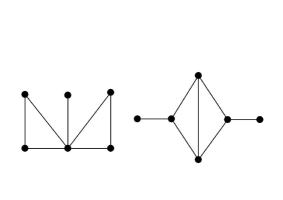
Figure 1: Two cospectral graphs but not cospectral with regard to ${\cal A}$

We identify the degree-adjacency matrix ${\cal A}$ with an endomorphism of the “vertex-space” of $\Gamma$, $l^{2}(V(\Gamma))$ which, for any given indexing of the vertices, is isomorphic to $\mathbb{R}^{n}$. Thus, for any vertex $v_{i}\in V(\Gamma)$, $e_{i}$ will denote the corresponding unit vector of the canonical base of $\mathbb{R}^{n}$.

If for two vertices $v_{i},v_{j}\in V(\Gamma)$ we have $\partial(v_{i},v_{j})>k$ then $({\cal A}^{k}(\Gamma))_{ij}=0$. Thus, for a real polynomial $P$ of degree $k$, we have

$$\partial(v_{i},v_{j})>k\Rightarrow P({\cal A}(\Gamma))_{ij}=0.$$ (1)

Through this fact we will study the $(\alpha,\beta,s,t)$-diameter of $\Gamma$ by using the degree-adjacency matrix (or its eigenvalues) and the $k$-alternating polynomials.

Another application of the degree-adjacency matrix can be found in [11] where spectral-like bounds on the higher Randić index $R_{2}(\Gamma)$ are given.

3 Alternating polynomials

The k-alternating polynomials, defined and studied in [5] by Fiol, Garriga and Yebra, can be defined as follows: let ${\cal M}=\{\mu_{1}>\cdots>\mu_{b}\}$ be a mesh of real numbers. For any $k=0,1,...,b-1$ let $P_{k}$ denote the k-alternating polynomial associated to ${\cal M}$. That is, the polynomial of $\mathbb{R}_{k}[x]$ such that

$$P_{k}(\mu)=\sup_{P\in\mathbb{R}_{k}[x]}\left\{P(\mu):\|P\|_{\infty}\leq 1\right\}$$

where $\mu$ is any real number greater than $\mu_{1}$ and $\|P\|_{\infty}={\displaystyle\max_{1\leq i\leq b}}\{|P(\mu_{i})|\}$. We collect here some of its main properties, referring the reader to [5] for a more detailed study.

• For any $k=0,1,...,b-1$ there is a unique $P_{k}$ which, moreover, is independent of the value of $\mu(>\mu_{1})$;

• $P_{k}$ has degree k;

• $P_{0}(\mu)=1<P_{1}(\mu)<\cdots<P_{b-1}(\mu)$;

• $P_{k}$ takes $k+1$ alternating values $\pm 1$ at the mesh points;

• There are explicit formulae for $P_{0}(=1),$ $P_{1},$ $P_{2},$ and $P_{b-1},$ while the other polynomials can be computed by solving a linear programming problem (for instance by the simplex method).

Hereafter the different eigenvalues of ${\cal A}$ will be denoted by $\lambda_{0}=1,\lambda_{1},\cdots,\lambda_{b}$ with $\lambda_{0}=1>\lambda_{1}>\cdots>\lambda_{b}$.

Proposition 1.

Let $\Gamma$ be a simple and connected graph. Let $P_{k}$ be the $k$-alternating polynomial associated to the mesh ${\cal M}=\{\lambda_{1}>\cdots>\lambda_{b}\}$ of degree-adjacency eigenvalues of $\Gamma$. Let $\nu$ be an eigenvector belonging to the eigenvalue $\lambda_{0}=1$. If $z\in\nu^{\perp}$ then $\|P_{k}({\cal A}(\Gamma))z\|\leq\|P_{k}\|_{\infty}\|z\|$.

Proof.

Using the following decomposition of the vector $z$

$$z=\sum_{l=1}^{b}z_{l},\quad\mbox{were}\quad z_{l}\in\mbox{\rm Ker}({\cal A}-\lambda_{l}{\bf I}).$$

we obtain

$$\left\|P_{k}({\cal A})z\right\|^{2} =\left\|P_{k}({\cal A})\sum_{l=1}^{b}z_{l}\right\|^{2}=\left\|\sum_{l=1}^{b}P_{k}(\lambda_{l})z_{l}\right\|^{2}$$

$$=\sum_{l=1}^{b}(P_{k}(\lambda_{l}))^{2}\|z_{l}\|^{2}\leq\|P_{k}\|_{\infty}^{2}\sum_{l=1}^{b}\|z_{l}\|^{2}=\|P_{k}\|_{\infty}^{2}\|z\|^{2}.$$

Hence, the result follows. ∎

Recently, the $k$-alternating polynomials have been successfully applied to the study of several parameter related to the concept of distance in graphs and hypergraphs. For instance, we cite [5, 6, 7, 8, 9, 10]. We emphasize the following result on the $(s,t)$-diameter [6]

$$P_{k}(\lambda)>\sqrt{\left(\frac{\|v\|^{2}}{s}-1\right)\left(\frac{\|{v}\|^{2}}{t}-1\right)}\Rightarrow D_{(s,t)}(\Gamma)\leq k,$$ (2)

where $P_{k}$ denotes the $k$-alternating polynomials on the mesh of eigenvalues of the standard adjacency matrix of $\Gamma$, $\lambda$ denotes the largest eigenvalue of $\Gamma$, and ${v}$ the eigenvector associated to $\lambda$ with minimum component 1. In the case of regular graphs, as v= j, the all-1 vector, the result (2) simplifies to

$$P_{k}(\lambda)>\sqrt{\left(\frac{n}{s}-1\right)\left(\frac{n}{t}-1\right)}\Rightarrow D_{(s,t)}(\Gamma)\leq k,$$ (3)

where $n=|V(\Gamma)|.$

4 Bounding the $(\alpha,\beta,s,t)$-diameter

Lemma 2.

Let $\Gamma$ be a simple and connected graph of size $m$. Let $P_{k}$ be the $k$-alternating polynomial associated to the mesh ${\cal M}=\{\lambda_{1}>\cdots>\lambda_{b}\}$ of degree-adjacency eigenvalues of $\Gamma$. Let $S=\{v_{i_{1}},v_{i_{2}},...,v_{i_{s}}\}$ and $T=\{v_{j_{1}},v_{j_{2}},...,v_{j_{t}}\}$ be two sets of vertices of $\Gamma$, and let $\rho_{s}=\left(\sum_{l=1}^{s}\sqrt{\delta(v_{i_{l}})}\right)^{2}$, $\rho_{t}=\left(\sum_{r=1}^{t}\sqrt{\delta(v_{j_{r}})}\right)^{2}$. Then,

$$P_{k}(1)>\sqrt{\left(\frac{2ms}{\rho_{s}}-1\right)\left(\frac{2mt}{\rho_{t}}-1\right)}\Rightarrow\partial(S,T)\leq k.$$

Proof.

Let $\sigma=\sum_{l=1}^{s}e_{i_{l}}$ and $\tau=\sum_{r=1}^{t}e_{j_{r}}$ be the vectors of $\mathbb{R}^{n}$ associated to the sets $S$ and $T$. Using the following decomposition

$$\sigma=\frac{\langle\sigma,\nu\rangle}{\|\nu\|^{2}}\nu+u=\frac{\sqrt{\rho_{s}}}{2m}\nu+u,\quad\tau=\frac{\langle\tau,\nu\rangle}{\|\nu\|^{2}}\nu+w=\frac{\sqrt{\rho_{t}}}{2m}\nu+w,$$ (4)

where $\nu=(\sqrt{\delta_{1}},\sqrt{\delta_{2}},...,\sqrt{\delta_{n}})$ and $u,w\in\nu^{\perp},$ we obtain

$$\partial(S,T)>k \Rightarrow\langle P_{k}({\cal A})\sigma,\tau\rangle=0$$

$$\Rightarrow P_{k}(1)\frac{\sqrt{\rho_{s}\rho_{t}}}{2m}=-\langle P_{k}({\cal A})u,w\rangle.$$

Thus, by the Cauchy-Schwarz inequality we have

$$\partial(S,T)>k\Rightarrow P_{k}(1)\frac{\sqrt{\rho_{s}\rho_{t}}}{2m}\leq\|P_{k}({\cal A})u\|\|w\|,$$

and by Proposition 1 we obtain

$$\partial(S,T)>k\Rightarrow P_{k}(1)\frac{\sqrt{\rho_{s}\rho_{t}}}{2m}\leq\|P_{k}\|_{\infty}\|u\|\|w\|.$$ (5)

Moreover, the decomposition (4) leads to

$$s=\|\sigma\|^{2}=\frac{\rho_{s}}{2m}+\|u\|^{2}\Rightarrow\|u\|=\sqrt{s-\frac{\rho_{s}}{2m}}$$

and

$$t=\|\tau\|^{2}=\frac{\rho_{t}}{2m}+\|w\|^{2}\Rightarrow\|w\|=\sqrt{t-\frac{\rho_{t}}{2m}}$$

So, by (5), we obtain

$$\partial(S,T)>k\Rightarrow P_{k}(1)\sqrt{\rho_{s}\rho_{t}}\leq\sqrt{(2ms-\rho_{s})(2mt-\rho_{t})}.$$ (6)

The converse of (6) leads to the result. ∎

Theorem 3.

Let $\Gamma$ be a simple and connected graph of size $m$. Let $P_{k}$ be the $k$-alternating polynomial associated to the mesh ${\cal M}=\{\lambda_{1}>\cdots>\lambda_{b}\}$ of degree-adjacency eigenvalues of $\Gamma$. Then,

$$P_{k}(1)>\sqrt{\left(\frac{2m}{s\alpha}-1\right)\left(\frac{2m}{t\beta}-1\right)}\Rightarrow D^{(\alpha,\beta)}_{(s,t)}\leq k.$$ (7)

Proof.

Consider $S,T\subset V(\Gamma)$ such that $|S|\geq s$, $\delta(S)\geq\alpha$, $|T|\geq t$ and $\delta(T)\geq\beta$. Then we have

$$\rho_{s}=\left(\sum_{u\in S}\sqrt{\delta(u)}\right)^{2}\geq s^{2}\alpha\quad{\rm and}\quad\rho_{t}=\left(\sum_{v\in T}\sqrt{\delta(v)}\right)^{2}\geq t^{2}\beta.$$

Hence,

$$\left(\frac{2m}{s\alpha}-1\right)\left(\frac{2m}{t\beta}-1\right)\geq\left(\frac{2ms}{\rho_{s}}-1\right)\left(\frac{2mt}{\rho_{t}}-1\right).$$

Therefore, by Lemma 2 the result follows. ∎

As we can see in the following examples, the above bound is attained for several values of the related parameters.

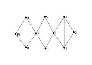
Figure 2:

Example 4.

The graph of Figure 2 has degree-adjacency eigenvalues:

$\left\{1,\frac{1+\sqrt{19}}{6},0.5358...,0,0,-\frac{1}{3},-\frac{1}{3},-0.3765...,\frac{1-\sqrt{19}}{6},-0.8259...\right\}$

from which we obtain $P_{4}(1)=3,89$, $P_{5}(1)=12,2$ and $P_{6}(1)=266,5$. Thus, the following bounds are attained: $D(\Gamma)=D_{(1,1)}^{(2,2)}(\Gamma)=D^{(2,2)}(\Gamma)\leq 6$, $D_{(1,1)}^{(2,3)}(\Gamma)=D^{(2,3)}(\Gamma)\leq 5$, $D_{(1,2)}^{(2,3)}(\Gamma)\leq 5$, $D_{(2,2)}^{(3,3)}(\Gamma)\leq 4$ and $D_{(3,3)}^{(2,2)}(\Gamma)=D_{(3,3)}(\Gamma)\leq 4$.

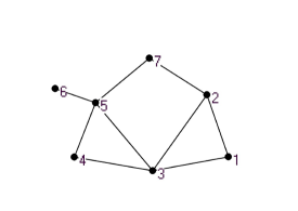
Figure 3:

Example 5.

The graph of Figure 3 has degree-adjacency eigenvalues:

$\left\{1,\frac{-3+\sqrt{249}}{24},\frac{1}{4},0,-\frac{1}{2},-\frac{1}{2},\frac{-3-\sqrt{249}}{24}\right\}$

from which we obtain $P_{1}(1)=1.7$, $P_{2}(1)=5$, $P_{3}(1)=15.2$ and $P_{4}(1)=58$. Thus, the following bounds are attained:

$D^{(1,2)}(\Gamma)\leq 3$, $D^{(3,4)}(\Gamma)\leq 2$ and $D^{(4,4)}(\Gamma)\leq 1$.

As particular cases of above theorem we derive the following results in which the expression (7) is simplified.

Corollary 6.

Let $\Gamma=(V,E)$ be a simple and connected graph of order $n$ and size $m$. Let $P_{k}$ be the $k$-alternating polynomial associated to the mesh ${\cal M}=\{\lambda_{1}>\cdots>\lambda_{b}\}$ of degree-adjacency eigenvalues of $\Gamma$. Then,

• $P_{k}(1)>\frac{2m}{\alpha}-1\Rightarrow D^{(\alpha,\alpha)}(\Gamma)\leq k.$

• The standard diameter is bounded by
  $P_{k}(1)>\frac{2m}{\delta}-1\Rightarrow D(\Gamma)\leq k.$

• If $\Gamma$ is regular, the standard diameter is bounded by
  $P_{k}(1)>n-1\Rightarrow D(\Gamma)\leq k.$

• If $\Gamma$ is an unicyclic graph, i.e., a connected graph containing exactly one cycle, the standard diameter is bounded by
  $P_{k}(1)>2n-1\Rightarrow D(\Gamma)\leq k.$

• If $\Gamma$ is regular, the $(s,t)$-diameter is bounded by

  $$P_{k}(1)>\sqrt{\left(\frac{n}{s}-1\right)\left(\frac{n}{t}-1\right)}\Rightarrow D_{(s,t)}(\Gamma)\leq k.$$

The bound (c) is an analogous result to the previous one given by Fiol, Garriga and Yebra in [5] by using the standard adjacency matrix. Moreover, bound (e) is an analogous result to (3).

4.1 Cutsets

Now we are going to give some other consequences of above study involving sets of vertices of equal cardinality and cut sets.

Proposition 7.

Let $\Gamma=(V,E)$ be a simple and connected graph of size $m$. Let $P_{k}$ be the $k$-alternating polynomial associated to the mesh ${\cal M}=\{\lambda_{1}>\cdots>\lambda_{b}\}$ of degree-adjacency eigenvalues of $\Gamma$. Let $S_{1},S_{2}\subset V(\Gamma)$ such that $|S_{1}|=|S_{2}|=s$, $\partial(S_{1},S_{2})>k$ and $\delta(v)\geq\alpha$ for all $v\in S_{1}\cup S_{2}$. Then

$$s\leq\left\lfloor\frac{2m}{\alpha(P_{k}(1)+1)}\right\rfloor\cdot$$ (8)

Proof.

Taking $\alpha=\beta$ and $s=t$, the converse of (7) gives

$$\partial(S_{1},S_{2})>k\Rightarrow P_{k}(1)\leq\frac{2m}{s\alpha}-1.$$

Solving for $s$, and considering that it is an integer, we obtain the result. ∎

Example 8.

To show the tightness of above bound we consider again the graph of Figure 2. For instance, taking $s=|S_{1}|=|S_{2}|$, $\partial(S_{1},S_{2})>5$ and $\delta(v)\geq 2$ for all $v\in S_{1}\cup S_{2}$, we obtain $s\leq 1.$ Moreover, as for this graph $P_{3}(1)=2,33$, in the case of $\partial(S_{1},S_{2})>3$ and $\delta(v)\geq 3$ for all $v\in S_{1}\cup S_{2}$, we obtain $s\leq 2$.

Note that, as in Proposition 7, if there are two sets $S_{1},S_{2}\subset V(\Gamma)$ such that $|S_{1}|=|S_{2}|=s$, $\partial(S_{1},S_{2})>k$ and $\delta(v)\geq\alpha$ for all $v\in S_{1}\cup S_{2}$, then

$$\alpha\leq\left\lfloor\frac{2m}{s(P_{k}(1)+1)}\right\rfloor\cdot$$ (9)

In the case of regular graphs, Proposition 7 allows us to derive the following result.

Corollary 9.

Let $\Gamma$ be a regular graph of order $n$. Let $S_{1},S_{2}\subset V(\Gamma)$ such that $|S_{1}|=|S_{2}|=s$ and $\partial(S_{1},S_{2})>k$. Then

$$s\leq\left\lfloor\frac{n}{P_{k}(1)+1}\right\rfloor\cdot$$ (10)

The above result is analogous to the previous one given by Yebra and the author in [9], for not necessarily regular graphs, by using the standard Laplacian matrix. These result becomes the main tool to the study of cut sets in [8].

A $k$-vertex separator is a subset $T_{k}\subset V(\Gamma)$ whose deletion separates $V(\Gamma)$ into two sets of equal cardinality, that are at distance greater than $k$. We denote by $vs_{k}(\Gamma)$ the minimum cardinality among all $k$-vertex separators, that is,

$$vs_{k}(\Gamma)=\min\{|T_{k}|:T_{k}\mbox{\rm\mbox{ } is a $k$-vertex separator of }\Gamma\}.$$

In [8] were obtained bounds on $vs_{k}(\Gamma)$ by using the $k$-alternating polynomials and the standard Laplacian spectrum. Proposition 7 allows us to study a particular case of vertex separator: a $(\alpha,k)$-vertex separator is a vertex set whose deletion separates $V(\Gamma)$ into two sets, $U$ and $W$, of equal cardinality whose minimum vertex degree is $\alpha$, such that $\partial(U,W)>k$. We denote by $vs_{(\alpha,k)}(\Gamma)$, the minimum cardinality among all $(\alpha,k)$-vertex separators.

Corollary 10.

Let $\Gamma=(V,E)$ be a simple and connected graph of order $n$ and size $m$. Let $P_{k}$ be the $k$-alternating polynomial associated to the mesh ${\cal M}=\{\lambda_{1}>\cdots>\lambda_{b}\}$ of degree-adjacency eigenvalues of $\Gamma$. Then

$$vs_{(\alpha,k)}(\Gamma)\geq n-2\left\lfloor\frac{2m}{\alpha(P_{k}(1)+1)}\right\rfloor\cdot$$ (11)

5 Laplacian matrix

Now we consider the Laplacian matrix, L, defined by Fan R. K. Chung as $\emph{L}=I-{\cal A}$, where $I$ denotes the identity matrix.

We denote by $\mu_{0}=0<\mu_{1}<\cdots<\mu_{b}$ the different eigenvalues of L. Thus, the eigenvalues of both matrices, L and ${\cal A}$, are related by

$$\mu_{l}=1-\lambda_{l},\quad l=0,1,...,b.$$

Notice also that the eigenvalue $\mu_{0}=0$ has eigenvector $\nu=(\sqrt{\delta_{1}},...,\sqrt{\delta_{n}})$ and multiplicity one in the case of connected graphs. Hence, both matrices, ${\cal A}$ and L, lead to equivalent spectral-like results. Particularly, the following theorem is the analogous of Theorem 7. The proof is basically as before.

Theorem 11.

Let $\Gamma=(V,E)$ be a simple and connected graph of size $m$. Let $P_{k}$ be the $k$-alternating polynomial associated to the mesh ${\cal M}=\{\mu_{1}<\cdots<\mu_{b}\}$ of $\emph{L}=\emph{L}(\Gamma)$. Then,

$$P_{k}(0)>\sqrt{\left(\frac{2m}{s\alpha}-1\right)\left(\frac{2m}{t\beta}-1\right)}\Rightarrow D^{(\alpha,\beta)}_{(s,t)}(\Gamma)\leq k.$$

We recall that if we use the standard adjacency matrix and the standard Laplacian matrix, the results are equivalent only in the regular case. In this sense, a comparative study was done in [7].

References

- [1] C. Balbuena, A. Carmona, J. Fábrega and M. A. Fiol, On the connectivity and the conditional diameter of graphs and digraphs. Networks 28 (2) (1996) 97-105.
- [2] C. Balbuena, J. Fábrega, X. Marcote and I. Pelayo, Superconnected digraphs and graphs with small conditional diameters, Networks 39 (3) (2002) 153-160.
- [3] A. Carmona and J. Fábrega, On the superconnectivity and the conditional diameters of graphs and digraphs, Networks 34 (3) (1999) 197-205.
- [4] F. R. K. Chung, Spectral Graph Theory. Conference Board of the Mathematical Sciences, n. 92, AMS, (1997).
- [5] M.A. Fiol, E. Garriga and J.L.A. Yebra, On a class of polynomials and its relation with the spectra and diameters of graphs, J. Combin. Theory Ser. B 67 (1996) 48-61.
- [6] M.A. Fiol, E. Garriga and J.L.A. Yebra, The alternating polynomial and their relation with the spectra and conditional diameters of graphs, Discrete Mathematics 167/168 (1997) 297-307.
- [7] J. A. Rodríguez and J. L. A. Yebra, Bounding the diameter and the mean distance of a graph from its eigenvalues: Laplacian versus adjacency matrix methods. Discrete Mathematics 196 (1999) 267-275.
- [8] J. A. Rodríguez, A. Gutiérrez and J. L. A. Yebra, On spectral bounds for cutsets Discrete Mathematics. 257 (1) (2002) 101-109.
- [9] J. A. Rodríguez and J.L.A. Yebra, Laplacian eigenvalues and the excess of a graph ARS Combinatoria. 64 (2002) 249-258.
- [10] J. A. Rodríguez. On the Laplacian eigenvalues and metric parameters of hypergraphs. Linear and Multilinear Algebra. 50 (1) (2002) 1-14.
- [11] J. A. Rodríguez. A spectral approach to the Randić index. Linear Algebra and its Applications 400 (2005) 339-344.