The Spectral Basis and Rational Interpolation

Abstract

The Euclidean Algorithm is the often forgotten key to rational approximation techniques, including Taylor, Lagrange, Hermite, osculating, cubic spline, Chebyshev, Padé and other interpolation schemes. A unified view of these various interpolation techniques is eloquently expressed in terms of the concept of the spectral basis of a factor ring of polynomials. When these methods are applied to the minimal polynomial of a matrix, they give a family of rational forms of functions of that matrix.

1 The Euclidean Algorithm and Spectral Basis

The euclidean algorithm has many important well-known consequences in number theory, algebra and analysis. In the spirit of [1], we are mainly interested here in some of its consequences regarding interpolation of functions over the real or complex numbers. Let $I\!\!R[x]$ and ${C\kern-6.47003ptI}[z]$ denote the rings of real-valued and complex-valued polynomials over the real and complex number fields $I\!\!R$ and ${C\kern-6.47003ptI}$, respectively. Whereas we state our results in terms of polynomials over the field of real numbers $I\!\!R$, all of the results are equally valid for polynomials over ${C\kern-6.47003ptI}$.

Let $h(x)$ denote the monic polynomial defined by

$$h(x)=\prod_{i=1}^{r}(x-x_{i})^{m_{i}},$$ (1)

where $\{x_{1},\ldots,x_{r}\}$ are the distinct real roots of $h(x)$ with multiplicities $\{m_{1},\ldots,m_{r}\}$, respectively. Let $f(x)\in I\!\!R[x]$ be any polynomial in $I\!\!R[x]$. Then the euclidean algorithm simply tells us that there will always exist polynomials $g(x)$ and a remainder $r(x)$ such that

$$f(x)=g(x)h(x)+r(x)$$ (2)

where $0\leq\deg(r(x))<\deg(h(x))$ or $r(x)\equiv 0$. When equation (2) holds, we say that $f(x)=r(x)\ {\rm mod}(h)$ where $h=h(x)$, or more concisely, that $f(x){\ \buildrel\rm h\over{=}\ }r(x)$. We denote the ring of all real polynomials modulo $h(x)$ by $I\!\!R[x]_{h}$. In the terminology of factor rings, $I\!\!R[x]_{h}\widetilde{=}I\!\!R[x]/\!\!<\!h(x)\!>$, meaning that $I\!\!R[x]_{h}$ is isomorphic to the factor ring $I\!\!R[x]/\!\!<\!h(x)\!>$ of $I\!\!R[x]$ generated by the principal ideal $<h(x)>$, [3, p.266]. Thus, $I\!\!R[x]_{h}$ has the structure of a ring with addition and multiplication of polynomials defined modulo $h(x)$.

By the standard basis of residue classes of $I\!\!R[x]_{h}$ we mean

$${\cal B}_{h}=\{1,x,x^{2},\ldots,x^{m-1}\},$$ (3)

where $m=\deg(h)=m_{1}+\ldots+m_{r}$. However, calculations in $I\!\!R[x]_{h}$ are much more simply carried out by appealing to the special properties of the spectral basis [7], [8]. The spectral basis ${\cal S}_{h}$ of $I\!\!R[x]_{h}$ consists of idempotents $s_{i}=s_{i}(x)$, and nilpotents $q_{i}=q_{i}(x)$ and their powers $q_{i}^{k}=q_{i}^{k}(x)$,

$${\cal S}_{h}=\{s_{1},q_{1},\ldots,q_{1}^{m_{1}-1},s_{2},q_{2},\ldots,q_{2}^{m_{2}-1},\ldots,s_{r},q_{r},\ldots,q_{r}^{m_{r}-1}\},$$ (4)

which satisfy the following properties under addition and multiplication in $I\!\!R[x]_{h}$ modulo $h(x)$:

1. $s_{1}+s_{2}+\cdots+s_{r}=1$, and $s_{i}s_{j}{\ \buildrel\rm h\over{=}\ }\delta_{ij}s_{i}$ for $i,j=1,\ldots,r$ where $\delta_{ij}=0$ for $i\neq j$ and $\delta_{ij}=1$ for $i=j$.

2. $q_{i}s_{i}{\ \buildrel\rm h\over{=}\ }q_{i}$, and $q_{i}^{m_{i}-1}\neq 0\ {\rm mod}(h)$ but $q_{i}^{m_{i}}{\ \buildrel\rm h\over{=}\ }0$, for $i=1,\ldots,r$.

3. For each $f(x)\in I\!\!R[x]$, $f(x)s_{i}{\ \buildrel\rm h\over{=}\ }\big{(}f(x){\rm mod}[(x-x_{i})^{m_{i}}]\big{)}s_{i}$ for $i=1,\ldots,r$.

Property 1, shows that the $s_{i}(x)$ are mutually annihilating idempotents which partition unity. Property 2, shows that $s_{i}$ acts as an identity element when multiplied by the nilpotent $q_{i}(x)$, and that $q_{i}(x)$ is a nilpotent of index $m_{i}$ in $I\!\!R[x]_{h}$. Property 3, shows that for each polynomial $f(x)\in I\!\!R[x]$, $s_{i}(x)$ acts as the projection of $f(x)$ onto the ring of polynomials $I\!\!R[x]_{(x-x_{i})^{m_{i}}}$ modulo $(x-x_{i})^{m_{i}}$.

From these three algebraic properties, we can explicitly solve for the polynomials that make up the spectral basis. For each $i=1,\ldots,r$, define $h_{i}=h_{i}(x)=h(x)/(x-x_{i})^{m_{i}}$. Using Properties 1 and 3, we find that

$$h_{i}s_{i}{\ \buildrel\rm h\over{=}\ }h_{i},$$ (5)

and since $h_{i}(x_{i})\neq 0$, it follows that $h_{i}^{-1}\neq 0\ {\rm mod}\ (x-x_{i})^{m_{i}}$. Multiplying both sides of equation (5) by $h_{i}^{-1}{\rm mod}\ (x-x_{i})^{m_{i}}$, we find that

$$s_{i}(x)=(h_{i}^{-1}{\rm mod}\ (x-x_{i})^{m_{i}})h_{i}(x),$$ (6)

which gives an explicit solution by taking the first $m_{i}$ terms of the Taylor series for $h_{i}^{-1}$ around the point $x=x_{i}$. Having found the idempotents $s_{i}$, the corresponding nilpotents $q_{i}$, and their powers, are specified by

$$q_{i}^{k}:{\ \buildrel\rm h\over{=}\ }(x-x_{i})^{k}s_{i}=(x-x_{i})^{k}(h_{i}^{-1}{\rm mod}\ (x-x_{i})^{m_{i}})h_{i}(x)$$

$${\ \buildrel\rm h\over{=}\ }(h_{i}^{-1}{\rm mod}\ (x-x_{i})^{m_{i}-k})h_{i}(x),$$ (7)

for $k=0,1,\ldots,m_{i}-1$. Note that for $k=0$, we get the correct convention that $q_{i}^{0}{\ \buildrel\rm h\over{=}\ }s_{i}$.

The transition from the standard basis (3) to the spectral basis (4) is accomplished by first noting that

$$x=\sum_{i=1}^{r}xs_{i}=\sum_{i=1}^{r}((x-x_{i})+x_{i})s_{i}{\ \buildrel\rm h\over{=}\ }\sum_{i=1}^{r}(x_{i}+q_{i})s_{i},$$ (8)

from which it follows that

$$x^{k}{\ \buildrel\rm h\over{=}\ }\sum_{i=1}^{r}(x_{i}+q_{i})^{k}s_{i}{\ \buildrel\rm h\over{=}\ }\sum_{i=1}^{r}\sum_{j=0}^{m_{i}-1}\pmatrix{k\cr j}x^{k-j}_{i}q_{i}^{j},$$

for $k=0,1,\ldots,m-1$, as easily follows by referring to the properties of the spectral basis [8].

2 Rational Interpolation

Let $f(x)$ be a real-valued function which is continuous and has derivatives to the orders $\{m_{1}-1,\ldots,m_{r}-1\}$ at the respective points $\{x_{1},\ldots,x_{r}\}$, where $\{x_{1},\ldots,x_{r}\}$ are the distinct real roots of $h(x)$ with multiplicities $\{m_{1},\ldots,m_{r}\}$ as was defined in (1) of the previous section.

The function $f(x)$ of the real variable $x$ can be extended to a function of the variable $x\in I\!\!R[x]_{h}$ by simply substituting (8) into $f(x)$, getting

$$f(x):=f(\sum_{i=1}^{r}(x_{i}+q_{i})s_{i}){\ \buildrel\rm h\over{=}\ }\sum_{i=1}^{r}f(x_{i}+q_{i})s_{i}.$$ (9)

If we now expand $f(x_{i}+q_{i})$ in a Taylor series about $x=x_{i}$, we get the desired expression

$$f(x_{i}+q_{i}){\ \buildrel\rm h\over{=}\ }\sum_{k=0}^{m_{i}-1}\frac{1}{k!}f^{(k)}(x_{i})q_{i}^{k},$$ (10)

where as usual, $f^{(k)}(x_{i})=\frac{d^{k}}{dx^{k}}f(x)|_{x=x_{i}}$. Although we have derived equations (9) and (10) modulo $h(x)$ from the basic properties of the spectral basis (4), we could equally well have taken (9) and (10) to be the definition of $f(x)$ modulo $h(x)$.

The interpolation polynomial

$$g(x)=f(x)\ {\rm mod}\ h(x){\ \buildrel\rm h\over{=}\ }\sum_{i=1}^{r}[\sum_{k=0}^{m_{i}-1}\frac{1}{k!}f^{(k)}(x_{i})q_{i}^{k}]s_{i}$$ (11)

is called the Birkhoff or osculating interpolation polynomial of $f(x)$ with respect to $h(x)$. In the special case that $m_{1}=\cdots=m_{r}=1$, $g(x)$ is called the Lagrange interpolation polynomial of $f(x)$, and in the special case when $m_{1}=\ldots=m_{r}=2$, $g(x)$ is called the Hermite interpolation polynomial of $f(x)$, [5, pps.278,287], [9, p.52]. When $r=1$, $g(x)$ reduces to the first $m_{1}-1$ terms of the Taylor series of $f(x)$ about $x=x_{1}$.

Rational interpolation also takes an equally eloquent form when expressed in terms of the spectral basis [9, p.58],[2]. Let $a(x)=\sum_{i=0}^{m-1}a_{i}x^{i}$, and $b(x)=\sum_{j=0}^{m-1}b_{j}x^{j}$ be polynomials over the real numbers $I\!\!R$. We say that

$$g(x)=\frac{a(x)}{b(x)}$$ (12)

is a rational interpolate of $f(x)$ at the points (nodes) $\{x_{1},\ldots,x_{r}\}$ with multiplicities $\{m_{1},\ldots,m_{r}\}$ if

$$f(x)b(x)-a(x){\ \buildrel\rm h\over{=}\ }0.$$ (13)

The usual way of defining rational interpolation involves the solution of a system of linear equations for coefficients of the polynomials $a(x)$ and $b(x)$. Our definition is simpler and more direct in that it only requires that the modular relation (13) holds. When $b(x)$ has no common zeros with $h(x)$, the equation (13) is equivalent to

$$f(x){\ \buildrel\rm h\over{=}\ }a(x)b(x)^{-1}.$$ (14)

Essentially, each choice of the shape polynomial $b(x)$ in (13) and (14) determines a different rational interpolation $g(x)$ of $f(x)$, [13]. Because of the homogeneous nature of the rational interpolate (12), we can require that $b(x_{e})=1$ at some point $x_{e}$ which is chosen not to be one of the roots $x_{i}$ of $h(x)$ nor a zero of $f(x)$. Whereas equation (13) is defined modulo($h(x)$) using (9) and (10), equation (12) is an ordinary equality.

Chebyshev and other kinds of rational interpolation are defined simply by replacing the powers of $x^{k}$ of $x$ in $a(x)$ and $b(x)$ by the corresponding Chebyshev or other sets of orthogonal polynomials of the same order. A comprehensive study of the algebraic structure of rational functions has been undertaken by Luis Verde-Star in a series of papers [10, 11, 12]. Examples of the various kinds of interpolation will be given in Section 3.

Cubic spline interpolation can be defined parametrically in terms of the spectral basis ${\cal S}_{2,2}$ of $I\!\!R[t]_{h}$ for $h=h(t)=t^{2}(t-1)^{2}$. Using the formulas (6) and (7) from the previous section, we find that

$${\cal S}_{2,2}=\{s_{1}=(2t+1)(t-1)^{2},q_{1}=t(t-1)^{2},s_{2}=(3-2t)t^{2},q_{2}=t^{2}(t-1)\}.$$ (15)

The piecewise natural cubic spline $\{g_{1}(t_{1}),g_{2}(t_{2}),\ldots,g_{k-1}(t_{k-1})\}$, for $0\leq t_{i}<1$ and $k\geq 3$, connecting the successive points $\{{\mathbf{x}}_{1},{\mathbf{x}}_{2},\ldots,{\mathbf{x}}_{k}\}$ in $I\!\!R^{n}$, is defined by

$$g_{i}(t_{i})={\mathbf{x}}_{i}s_{1}(t_{i})+{\mathbf{v}}_{i}q_{1}(t_{i})+{\mathbf{x}}_{i+1}s_{2}(t_{i})+{\mathbf{v}}_{i+1}q_{2}(t_{i}),$$ (16)

with the requirements that

$$g_{1}^{\prime\prime}(0)=0=g_{k-1}^{\prime\prime}(1)\ \ {\rm and}\ \ g_{i}^{\prime\prime}(1)=g_{i+1}^{\prime\prime}(0)$$ (17)

for $i=1,\ldots,k-2$. Taking the second derivatives of $g_{i}(t_{i})$, and evaluating at $t_{i}=0,1$ gives

$$g_{i}^{\prime\prime}(0)=6({\mathbf{x}}_{i+1}-{\mathbf{x}}_{i})-4{\mathbf{v}}_{i}-2{\mathbf{v}}_{i+1},$$ (18)

and

$$g_{i}^{\prime\prime}(1)=-6({\mathbf{x}}_{i+1}-{\mathbf{x}}_{i})+2{\mathbf{v}}_{i}+4{\mathbf{v}}_{i+1}.$$ (19)

The resulting $k$ linear vector equations are uniquely solved for the $k$-unknown tangent vectors ${\mathbf{v}}_{1},{\mathbf{v}}_{2},\ldots,{\mathbf{v}}_{k}$.

If, instead of the requirement (17), the vectors ${\mathbf{v}}_{1}$ and ${\mathbf{v}}_{k}$ are taken as given, and the remaining $(k-2)$ linear vector equations

$$g_{i}^{\prime\prime}(1)=g_{i+1}^{\prime\prime}(0),$$ (20)

for $i=1,\ldots,k-2$, are uniquely solved for the $(k-2)$ unknown tangent vectors ${\mathbf{v}}_{2},{\mathbf{v}}_{2},\ldots,{\mathbf{v}}_{k-1}$, the resulting solution is called the bounded cubic spline, [9, p.93].

Various kinds of rational cubic splines can also be easily constructed by replacing the spectral basis ${\cal S}_{2,2}$ in (16) by a rational spectral basis of the form

$${\cal R}_{2,2}(b)=\{s_{r1},q_{r1},s_{r2},q_{r2}\}$$ (21)

for

$$s_{r1}(t)=\frac{b(t)s_{1}(t)\ {\rm mod}(h(t))}{b(t)},\ q_{r1}(t)=\frac{b(t)q_{1}(t)\ {\rm mod}(h(t))}{b(t)}$$

and

$$s_{r2}(t)=\frac{b(t)s_{2}(t)\ {\rm mod}(h(t))}{b(t)},\ q_{r2}(t)=\frac{b(t)q_{2}(t)\ {\rm mod}(h(t))}{b(t)},$$

where $b=b(t)=1+b_{1}t+b_{2}t^{2}+b_{3}t^{3}$ and $b(1)\neq 0$. Clearly, the rational spectral basis ${\cal R}_{2,2}(b)$ reduces to the ordinary spectral basis ${\cal S}_{2,2}$, given in (15), for $b=b(t)=1$. Of course, when using the rational spectral basis, the second derivatives $g_{i}^{\prime\prime}(0)$ and $g_{i}^{\prime\prime}(1)$, given in (18) and (19), must be recalculated.

3 Circles

A circle and other conics are good geometric figures on which to carry out interpolation experiments. We derive here several approximations for the unit circle, centered at the origin, using rational spectral bases.

The rational spectral basis ${\cal S}_{h}=\{s_{r1},s_{r2},s_{r3}\}$ for $b=1+b_{1}t+b_{2}t^{2}$ and $h(t)=(t+1)t(t-1)$, is defined by

$$s_{r1}=\frac{\frac{1}{2}(1-b_{1}+b_{2})t(t-1)}{1+b_{1}t+b_{2}t^{2}},s_{r2}=-\frac{(t-1)(t+1)}{1+b_{1}t+b_{2}t^{2}},$$

and

$$s_{r3}=\frac{\frac{1}{2}(1+b_{1}+b_{2})t(t+1)}{1+b_{1}t+b_{2}t^{2}}.$$

We wish to optimize (in the sense of least squares) the choice of $b_{1}$ and $b_{2}$ so that the interpolating curve $g(t)=f(-1)s_{r1}+f(0)s_{r2}+f(1)s_{r3}$ to the semi-circle $f(t)=\pmatrix{\cos(\pi t/2),\sin(\pi t/2)}$, for $-1\leq t\leq 1$ is as good as possible. The values of $b_{1}$ and $b_{2}$ can easily be found by requiring that $g(1/2)\cdot g(1/2)=1=g(-1/2)\cdot g(-1/2)$, giving the values $b_{1}=0$ and $b_{2}=\pm 1$. The value $b_{2}=-1$, gives the single point $(1,0)$, whereas $b_{2}=1$ gives the well-known parameterization of the circle $g(t)=(\frac{1-t^{2}}{1+t^{2}},\frac{2t}{1+t^{2}})$.

A family of rational approximations to the quarter unit circle through the nodes $(1,0)$ and $(0,1)$, with the initial and terminal tangent velocity vectors $(0,v)$ and $(-v,0)$, is specified by

$$g(t)=(1,0)s_{r1}+(0,v)q_{r1}+(0,1)s_{r2}+(-v,0)q_{r2},$$

in the rational spectral basis (21). One popular construction of the circle is based on NURBS (nonuniform rational B-splines) [9, p.110]. Letting $b_{1}=-2+\sqrt{2}=-b_{2}$, the choice $v=\sqrt{2}$ precisely eliminates the $t^{3}$ term in the numerator, and gives the nurb parameterization

$$g(t)=(1,0)s_{r1}+(0,\sqrt{2})q_{r1}+(0,1)s_{r2}+(-\sqrt{2},0)q_{r2}$$

$$=\Big{(}\frac{1+(-2+\sqrt{2})t+(1-\sqrt{2})t^{2}}{1+(-2+\sqrt{2})t+(2-\sqrt{2})t^{2}},\frac{\sqrt{2}t+(1-\sqrt{2})t^{2}}{1+(-2+\sqrt{2})t+(2-\sqrt{2}t^{2}}\Big{)}.$$

A quite different perfect parameterization of the unit circle through the interpolation points $(1,0)$ and $(0,1)$, and taking the initial tangent vector at $(1,0)$ to be $(0,\pi/2)$, can be derived by using the rational spectral basis of

$${\cal S}_{2,1}=\{s_{1}=-(t+1)(t-1),q_{1}=-(-1+t)t,s_{2}=t^{2}\}$$

for $h(t)=t^{2}(t-1)$. We find that

$$g(t)=\frac{(1,0)s_{1}+\Big{(}b_{1}(1,0)+(0,\frac{\pi}{2})\Big{)}q_{1}+(0,1)(1+b_{1}+b_{2})s_{2}}{1+b_{1}t+b_{2}t^{2}}$$

Optimizing $b_{1}$ and $b_{2}$, we find that

$$g(t)=\Big{(}\frac{8+4(\pi-4)t-4(\pi-2)t^{2}}{8+4(\pi-4)t+(\pi^{2}-4\pi+8)t^{2}},\frac{4\pi t+(\pi-4)\pi t^{2}}{8+4(\pi-4)t+(\pi^{2}-4\pi+8)t^{2}}\Big{)}.$$

Whereas the above parameterizations give perfect circles, there are many other parameterizations that are interesting. For example, consider the family of approximations to the unit semicircle through the points $(1,0)$ and $(-1,0)$, given by

$$g(t)=(1,0)s_{r1}+(0,v)q_{r1}+(-1,0)s_{r2}+(0,-v)q_{r1}$$

employing the rational spectral basis of the kind (21). Choosing $b=1-t+t^{2}$, and $v=3$ gives a very good approximation to the unit semicircle for $0\leq t\leq 1$,

$$g(t)=\Big{(}\frac{1-t-3t^{2}+2t^{3}}{1-t+t^{2}},\frac{-3(t-1)t}{1-t+t^{2}}\Big{)}\widetilde{=}(\cos\pi t,\sin\pi t).$$ (22)

with a least square error less than $.000071$, see figure 3.1

Fig. 1: The unit semicircle is shown together with its approximation.

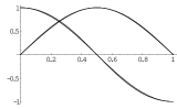
Fig. 2: Both sine and cosine curves are shown together with their approximations.

It is interesting to note that this parameterization also gives a good approximation to $\cos\pi t$ and $\sin\pi t$ for $0\leq t\leq 1$, see figure 3.2 The series expansions for the approximations to $\cos\pi t$ and $\sin\pi t$ are

$$\cos\pi t\widetilde{=}1-4t^{2}-2t^{3}+\sum_{k=1}^{\infty}(-1)^{k+1}[2t^{3k+1}+4t^{3k+2}+2t^{3k+3}]$$

and

$$\sin\pi t\widetilde{=}3t+3\sum_{k=1}^{\infty}(-1)^{k}[t^{3k}+t^{3k+1}],$$

which are interesting in their own right.

4 Matrices

Let $A$ be any $n\times n$ matrix over a field $\cal K$. The field $\cal K$ may be the real or complex numbers, or even a finite Galois field. It is well known that every matrix satisfies it’s characteristic polynomial, defined by

$$\varphi(x)=\det(xI-A),$$

where $I$ is the identity $n\times n$ matrix [6, 4]. The theory of a spectral basis is directly applicable to a matrix whenever the characteristic polynomial is of the form $\varphi(x)=\prod_{i=1}^{r}(x-x_{i})^{n_{i}}$ for distinct roots $x_{i}\in{\cal K}$. When applying the spectral basis to a matrix $A$, it is better to use the minimal polynomial $\psi(x)=\prod_{i=1}^{r}(x-x_{i})^{m_{i}}$, where $1\leq m_{i}\leq n_{i}$ for each $i=1,\ldots,r$. The minimal polynomial of the matrix $A$ is defined by the condition that it is unique monic polynomial of least degree for which $\psi(A)=0$.

Any of the interpolation formulas, developed in terms of the spectral basis in the previous sections, apply immediately to the matrix $A$, provided that $h(x)=\psi(x)$. This is because the relationship that $h(x)=0\ {\rm mod}\ h$ is precisely reflected in the condition that $\psi(A)=0$ for the minimal polynomial $\psi$ of the matrix $A$. Thus, the spectral form of the matrix $A$ is given by simply replacing $x$ by the matrix $A$ in (8), getting

$$A=\sum_{i=1}^{r}x_{i}s_{i}(A)+q_{i}(A)=\sum_{i=1}^{r}x_{i}S_{i}+Q_{i},$$ (23)

for $S_{i}=s_{i}(A)$ and $Q_{i}=q_{i}(A)$. The matrices $\{S_{i},Q_{i}\}$ of the spectral basis satisfy exactly the same rules under matrix addition and multiplication as does the polynomials $\{s_{i},q_{i}\}$ of the spectral basis modulo $h(x)$, [7].

For example, the matrix

$$A=\pmatrix{-2&-1&0&0\cr-1&5&1&1\cr-6&-5&-1&0\cr-8&-10&-3&0}$$

has both characteristic and minimal polynomials $h=t^{2}(t-1)$. As a consequence, we can apply all the above interpolation formulas, found for the rational spectral basis of $h(x)$, without modification. Using (11), (15), (22) and (23), we find that

$$\cos{\pi A}=I-6A^{2}+4A^{3}=\frac{I-A-3A^{2}+2A^{3}}{I-A+A^{2}}=\pmatrix{1&2&-10&6\cr-10&-3&26&-14\cr 10&8&-45&26\cr 20&14&-82&47}$$

and

$$\sin{\pi A}=A-A^{2}=\frac{-3A^{2}+3A}{I-A+A^{2}}=\pmatrix{21&-6&-3&-3\cr-48&18&0&12\cr 87&-27&-9&-15\cr 156&-51&-12&-30}.$$

As a check, we calculate $\cos^{2}\pi A+\sin^{2}\pi A=I$ as expected.

References

• [1] David A. Cox, What is the Role of Algebra in Applied Mathematics?, Notices of the American Mathematical Society 52, No. 10, November 2005, pp. 1193-1198.
• [2] P.J. Davis, Interpolation and Approximation, Dover Publications, New York, 1975.
• [3] J.A. Gallian, Contemporary Abstract Algebra, $6^{th}$ ed., Houghton Mifflin Company, Boston, 2006.
• [4] F.R. Gantmacher, Theory of Matrices, translated by K. A. Hirsch, Chelsea Publishing Co., New York, 1959.
• [5] R.W. Hamming, Numerical Methods for Scientists and Engineers, Dover Publications, Inc., New York, 1973.
• [6] R.A. Horn and C.R. Johnson, Topics in Matrix Analysis, Cambridge University Press, New York, 1991.
• [7] G. Sobczyk, The Missing Spectral Basis in Algebra and Number Theory, The American Mathematical Monthly 108 April 2001, pp. 336-346.
• [8] G. Sobczyk, Generalized Vandermonde Determinants and Applications, Aportaciones Matematicas, Serie Comunicaciones Vol. 30 (2002) 203 - 213.
• [9] J. Stoer and R. Bulirsch, Introduction to Numerical Analysis 2nd Ed., Translated by R. Bartels, W. Gautschi, and C. Witzgall, Springer-Verlag, New York, 1993.
• [10] L. Verde-Star, An Hopf Algebra Structure on Rational Functions, Advances in Mathematics 116, No. 2, December 1995, 377-388.
• [11] L. Verde-Star, An Algebraic Approach to Convolutions and Transform Methods, Adv. Appl. Math. 19 (1997) 117-143.
• [12] L. Verde-Star, Approximation and Optimization, in Proceedings of ICAOR: International Conference on Approximation and Optimization (Romania), I, Transilvania Press, 1997, pp. 121-138.
• [13] Qiang Wang and Jieqing Tan, Rational Quartic Spline Involving Shape Parameters, in Journal of Information & Computational Science 1: 1 (2004) 127-130, http://www.joics.com