A moving mesh method
with variable mesh relaxation time

Abstract

We propose a moving mesh adaptive approach for solving time-dependent partial differential equations. The motion of spatial grid points is governed by a moving mesh PDE (MMPDE) in which a mesh relaxation time $\tau$ is employed as a regularization parameter. Previously reported results on MMPDEs have invariably employed a constant value of the parameter $\tau$. We extend this standard approach by incorporating a variable relaxation time that is calculated adaptively alongside the solution in order to regularize the mesh appropriately throughout a computation. We focus on singular problems involving self-similar blow-up to demonstrate the advantages of using a variable relaxation time over a fixed one in terms of accuracy, stability and efficiency.

AMS Classification: 65M50, 65M06, 35K57

and

1 Introduction

Moving mesh methods have been employed widely to approximate solutions of partial differential equations which exhibit large solution variations, such as shock waves and boundary or interior layers. Several moving mesh approaches have been derived and many authors have discussed the significant improvements in accuracy and efficiency that can be achieved with respect to fixed mesh methods [9, 13, 14, 17, 20, 21, 22].

The moving mesh PDE (or MMPDE) approach has proven particularly effective in solving nonlinear PDEs that exhibit solutions having some type of singularity, such as self-similar blow-up [7] or moving fronts [3, 21]. For blow-up problems in particular, moving mesh methods permit a detailed study of the singularity formation with a degree of accuracy and efficiency that is simply not possible using fixed mesh methods. The primary advantage of the moving mesh approach stems from its ability to exploit special features of the solution (such as self-similarity) and build them directly into the numerical scheme.

In the MMPDE approach, a separate PDE is derived to evolve the mesh points in such a way that they tend towards an equidistributed mesh at steady state, in the sense that the mesh points are positioned in space so as to equally distribute some measure of the solution error. The MMPDE is coupled nonlinearly to the physical PDE of interest, and both PDEs are solved simultaneously. A key parameter in the moving mesh equation is the mesh relaxation time, usually denoted as $\tau$; the exact equidistribution equation is notoriously ill-conditioned [2, 19, 16] and so $\tau$ acts to regularize the mesh evolution in time. The philosophy behind introducing temporal smoothing, instead of equidistributing exactly, is that the mesh need not be solved to the same level of accuracy as the physical PDE; in fact, solution accuracy can still be significantly improved over fixed mesh methods by only approximately equidistributing the mesh.

In previous results reported in the literature, the mesh relaxation time is invariably taken to be a constant for any given simulation. Furthermore, Huang, Ren and Russell observed in [14] that “while the parameter $\tau$ is critical, in our experience the numerical methods are relatively insensitive to the actual choice of $\tau$ in applications,” and similar comments were made in [7, 13]. However, it is essential to keep in mind that these observations were made for problems in which the range of time scales present in the solution was fairly limited. In practice, $\tau$ must be tuned manually to optimize the behaviour of the computed mesh, and sometimes even to obtain a convergent numerical solution.

The main purpose of this paper is to consider situations where taking constant $\tau$ may not be appropriate. Keeping in mind that $\tau$ can be interpreted as a time scale for the mesh motion, then $\tau$ should in fact be taken as a solution-dependent parameter, because as singularities form, intensify, propagate, and dissipate, the speed of solution variations (and hence also of the mesh points) in a given computation may vary a great deal. By no means are we suggesting that a variable $\tau$ is necessary in all moving mesh calculations. Nonetheless, there is some advantage to be gained by having an algorithm that is capable of determining the value of $\tau$ automatically as part of the solution process without requiring the user to determine its value through trial and error (since the complicated nonlinear coupling between solution and mesh in the MMPDE approach means there is no way to know the value of $\tau$ a priori). The main purpose of this paper is to demonstrate, by means of specific examples, that varying the mesh relaxation parameter throughout a computation can be of significant advantage in terms of both accuracy and efficiency. We will present an approach for adaptively selecting $\tau$ in such a way that the temporal evolution of the mesh is optimal in an appropriate sense.

This paper is organized as follows. In Section 2, we briefly review moving mesh methods in which the mesh equation incorporates a relaxation time $\tau$. The main motivating example for introducing an adaptive strategy for choosing a time-dependent mesh smoothing parameter comes from a class of nonlinear parabolic equations exhibiting self-similar blow-up behaviour; we therefore introduce in Section 3 the blow-up model equation, and motivate a particular choice of $\tau(t)$ which is suggested by the analysis of blow-up problems. Numerical experiments are then presented in Section 4 to illustrate the advantages of this modified moving mesh approach in terms of both accuracy and efficiency.

2 The moving mesh method

The evolution of a moving computational grid can be viewed as a discretization of a one-to-one, time-dependent coordinate mapping. Let $x$ and $\xi$ denote the physical and computational coordinates respectively, and define a coordinate transformation by

$$x=x(\xi,t)\quad\text{where}\quad x(0,t)=0\quad\text{and}\quad x(1,t)=1,$$

where both $x$ and $\xi$ are assumed to lie in interval $[0,1]$. The computational coordinate is discretized on a uniform mesh given by $\xi_{i}=i/N$, where $i=0,1,2,\dots,N$ and $N$ is a positive integer. The corresponding non-uniform mesh is denoted by

$$0=x_{0}<x_{1}(t)<x_{2}(t)<\cdots<x_{N-1}(t)<x_{N}=1.$$

A key ingredient of the moving mesh approach is the monitor function, $M(x,t$), which is chosen to be some approximate measure of the solution error. For a given monitor function, the mesh point locations $x_{i}(t)$ could be required to satisfy the following equidistribution principle (EP) for all values of time $t$ [14]:

$$\int_{x_{i-1}(t)}^{x_{i}(t)}M(x,t)dx=\frac{1}{N}\int_{0}^{1}M(x,t)dx=\frac{\theta(t)}{N},$$

or equivalently

$$\int_{0}^{x_{i}(t)}M(x^{\prime},t)\,dx^{\prime}=\frac{i}{N}\theta(t)=\xi_{i}\,\theta(t),$$ (1)

where $\theta(t)=\int_{0}^{1}M(x^{\prime},t)\,dx^{\prime}$. This EP is intended to concentrate points in regions where $M$ (and hence also the solution error measure) is large, thereby placing fewer points in areas where the error is small. Differentiating (1) yields an equivalent differential form

$$\frac{\partial}{\partial\xi}\left(M\frac{\partial x}{\partial\xi}\right)(\xi,t)=0,$$ (2)

where $x(0,t)=0$ and $x(1,t)=1$.

Solving the elliptic equation (2) directly is often problematic, since it introduces a nonlinear coupling between the mesh and the solution through the dependence of $M$ on the solution $u$. Furthermore, when the physical and mesh PDEs are discretized, they take the form of an index-2 DAE system which is very stiff in practice and also typically ill-conditioned [2, 19, 16]. As a result, it is usually much more attractive to relax the requirement of exact equidistribution by introducing a relaxation time $\tau$ into the problem. A dynamic moving mesh equation can be derived by requiring the mesh to satisfy the above EP at a later time $t+\tau$ instead of at $t$. Because $\theta(t)$ has been eliminated from the differential form of the EP, the mesh must satisfy

$$\frac{\partial}{\partial\xi}\left[M\left(x(\xi,t+\tau),t+\tau\right)\,\frac{\partial}{\partial\xi}x(\xi,t+\tau)\right]=0.$$ (3)

By expanding the terms $\frac{\partial}{\partial\xi}x(\xi,t+\tau)$ and $M(x(\xi,t+\tau),t+\tau)$ in Taylor series and dropping certain higher order terms, a variety of different MMPDEs can be derived [14]. In this paper we will employ two specific moving mesh equations:

MMPDE4: $$\tau\frac{\partial}{\partial\xi}\left(M\frac{\partial\dot{x}}{\partial\xi}\right) =-\frac{\partial}{\partial\xi}\left(M\frac{\partial x}{\partial\xi}\right),$$ (4)

MMPDE6: $$\tau\frac{\partial^{2}\dot{x}}{\partial\xi^{2}} =-\frac{\partial}{\partial\xi}(M\frac{\partial x}{\partial\xi}).\hskip 56.9055pt$$ (5)

The relaxation parameter $\tau$ can also be thought of as introducing temporal smoothing into the mesh. The equivalent derivation for a time-dependent $\tau(t)$ is given in Appendix A.

The choice of monitor function $M$ in this method is somewhat arbitrary; in general, $M$ can be any given function of $u$, or it may also be based on some error estimate determined numerically based on discrete solution values. A commonly used monitor function is $M=\sqrt{1+u_{x}^{2}}$, which equidistributes the arclength of the solution $u$. However, this choice of $M$ often behaves very badly in simulations, concentrating too many points in singularities and making the coupled problem excessively stiff [16, 21]. Other common monitor function are chosen either for analytical reasons (such as the form $M=|u|^{p}$ for self-similar blow-up problems [7]) or for practical considerations (such as the component-averaged monitor developed in [21] for hyperbolic systems).

In this work, we discretize the mesh equation using centered finite differences in space, which yields for MMPDE6:

$$\dot{x}_{i+1}-2\dot{x}_{i}+\dot{x}_{i-1}=-\frac{E_{i}}{\tau}.$$ (6a)

The quantity $$E_{i}$$ represents a centered approximation to the term on the right hand side of MMPDE6 given by

$$E_{i}=M_{i+1/2}\left(x_{i+1}-x_{i}\right)-M_{i-1/2}\left(x_{i}-x_{i-1}\right),$$ (6b)

where $M_{i+1/2}={\textstyle\frac{1}{2}}(M_{i}+M_{i+1})$, $M_{i}=M(u_{i})$, and $u_{i}\approx u(x_{i},t)$ is an approximation of the solution at grid point $x_{i}$. The discretization for MMPDE4, which is also employed here, is carried out in a similar fashion. It turns out to be very important to smooth the monitor function in space as well as in time in order to avoid oscillatory errors in mesh locations which can then feed into the solution. To this end, the discrete monitor function values $M_{i}$ are usually replaced with smoothed versions

$$\widetilde{M_{i}}=\left(\frac{\sum_{j=i-ip}^{i+ip}M_{j}^{2}\left(\frac{\gamma}{1+\gamma}\right)^{|j-i|}}{\sum_{j=i-ip}^{i+ip}\left(\frac{\gamma}{1+\gamma}\right)^{|j-i|}}\right)^{1/2},$$ (7)

where $\gamma$ and $ip$ are parameters that must be chosen appropriately.

2.1 The effect of $\tau$ on mesh movement

Because of the importance of temporal smoothing in the present work, it is helpful to first consider some illustrative examples that elucidate the effect of $\tau$ on the computed mesh motion. For this purpose, we consider first three examples wherein $u(x,t)$ is a given function, so that the mesh equation is uncoupled from the physical PDE.

Example 1

We first consider

$$u(x,t)=e^{-10\pi^{2}t}\sin(\pi x),$$ (8)

for values of $x\in[0,1]$ and $t\in[0,10]$, which was used in [10] to study the stability of various moving mesh equations, and also as a numerical example in [14]. The mesh equation is chosen to be MMPDE6, which is discretized using standard centered finite differences. For the purposes of this example, we use the arclength monitor function $M=\sqrt{1+u_{x}^{2}}$ with spatial smoothing parameters $\gamma=2$ and $ip=4$. The spatial domain is divided into $N=100$ mesh points and the value of $\tau$ is taken to be a constant ranging from $10^{0}$ down to $10^{-5}$. The mesh points are initially uniformly distributed, so that the mesh undergoes a rapid initial transient as the grid points are driven towards equidistribution by the MMPDE. The speed of this initial transient is governed by the choice of the mesh relaxation time parameter. Also, since $u_{x}(x,t)\rightarrow 0$ in the limit as $t\rightarrow\infty$, then for the arclength monitor $M\rightarrow 1$ as $t\rightarrow+\infty$; therefore, the equidistributed mesh should tend over long times to a uniform mesh in space.

Figure 1 shows solution curves and Figure 2 the mesh trajectories (i.e., contours of $\xi(x,t)$) for the above example using MMPDE6 and a uniform initial mesh. These results demonstrate a few important points. First, the ability of the moving mesh to respond to rapid solution transients (in this case represented by the initial transient mesh redistribution) is governed in large part by the choice of $\tau$. In particular, if $\tau$ is taken too large, then the mesh is incapable of adapting sufficiently well to keep up with the solution, which is easily seen here in the case $\tau=10^{-1}$. Secondly, once $\tau$ is taken small enough, there is no longer any significant change in the mesh locations, as seen by comparing the mesh trajectories when $\tau=10^{-3}$ and $\tau=10^{-5}$ (ignoring the initial transients which are not physical but driven solely by the artificially chosen initial uniform mesh). When $\tau$ is taken smaller than $10^{-5}$ there is no visible change in either the computed mesh or the time stepping behaviour.

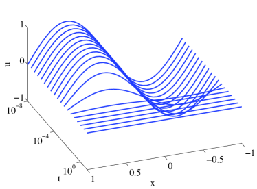
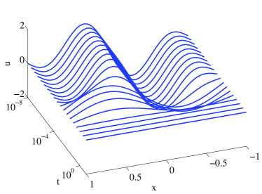
Figure 1: Solution profiles for the function (8) used in Example 1 (left) and (9) from Example 2 (right).

$\tau=10^{-1}$, $\text{CPU}=7\;s$	$\tau=10^{-3}$, $\text{CPU}=12\;s$	$\tau=10^{-5}$, $\text{CPU}=13\;s$
\psfrag{x}[c][b]{$x$}\psfrag{t}[Bc][c]{$t$}\psfrag{ t}[Bc][c]{$\Delta t$}\psfrag{D}{}\psfrag{Mesh trajectories}{}\psfrag{Time step}{}\includegraphics[width=130.08731pt]{u1-2-xt.eps}	\psfrag{x}[c][b]{$x$}\psfrag{t}[Bc][c]{$t$}\psfrag{ t}[Bc][c]{$\Delta t$}\psfrag{D}{}\psfrag{Mesh trajectories}{}\psfrag{Time step}{}\includegraphics[width=130.08731pt]{u1-3-xt.eps}	\psfrag{x}[c][b]{$x$}\psfrag{t}[Bc][c]{$t$}\psfrag{ t}[Bc][c]{$\Delta t$}\psfrag{D}{}\psfrag{Mesh trajectories}{}\psfrag{Time step}{}\includegraphics[width=130.08731pt]{u1-4-xt.eps}
\psfrag{x}[c][b]{$x$}\psfrag{t}[Bc][c]{$t$}\psfrag{ t}[Bc][c]{$\Delta t$}\psfrag{D}{}\psfrag{Mesh trajectories}{}\psfrag{Time step}{}\psfrag{t}[c][b]{$t$}\includegraphics[width=130.08731pt]{u1-2-dt.eps}	\psfrag{x}[c][b]{$x$}\psfrag{t}[Bc][c]{$t$}\psfrag{ t}[Bc][c]{$\Delta t$}\psfrag{D}{}\psfrag{Mesh trajectories}{}\psfrag{Time step}{}\psfrag{t}[c][b]{$t$}\includegraphics[width=130.08731pt]{u1-3-dt.eps}	\psfrag{x}[c][b]{$x$}\psfrag{t}[Bc][c]{$t$}\psfrag{ t}[Bc][c]{$\Delta t$}\psfrag{D}{}\psfrag{Mesh trajectories}{}\psfrag{Time step}{}\psfrag{t}[c][b]{$t$}\includegraphics[width=130.08731pt]{u1-4-dt.eps}

Figure 2: Mesh trajectories (top) and time step histories (bottom) for the given solution (8) (Example 1) with various values of $\tau$ using MMPDE6 and the arclength monitor function.

Example 2

A function which provides a more stringent test of a moving mesh calculation is

$$u(x,t)=e^{-\pi^{2}t}\sin(\pi x)+e^{-(10\pi)^{2}t}\sin(2\pi x),$$ (9)

which is a slight modification of (8) having two widely-separated time scales over which the solution varies. Notice in the results depicted in Figure 3 that the more rapid variation embodied by the second term in (9) is only really well-captured in the mesh for the smallest value of $\tau=10^{-5}$. When the fast term dies out shortly after time $t=10^{-4}\;s$, then the mesh redistributes to resolve the remaining single peak.

$\tau=10^{-1}$, $\text{CPU}=11\;s$	$\tau=10^{-3}$, $\text{CPU}=17\;s$	$\tau=10^{-5}$, $\text{CPU}=27\;s$
\psfrag{x}[c][b]{$x$}\psfrag{t}[Bc][c]{$t$}\psfrag{Mesh trajectories}{}\includegraphics[width=130.08731pt]{u3-1-xt.eps}	\psfrag{x}[c][b]{$x$}\psfrag{t}[Bc][c]{$t$}\psfrag{Mesh trajectories}{}\includegraphics[width=130.08731pt]{u3-3-xt.eps}	\psfrag{x}[c][b]{$x$}\psfrag{t}[Bc][c]{$t$}\psfrag{Mesh trajectories}{}\includegraphics[width=130.08731pt]{u3-5-xt.eps}

Figure 3: Mesh trajectories for the given solution (9) (Example 2) using MMPDE6 and the arclength monitor function.

Example 3

We next consider the following Gaussian function which blows up at the point $x=x^{\ast}$ as $t\rightarrow t^{\ast}$

$$u(x,t)=\frac{1}{\sqrt{4\pi(t^{\ast}-t)}}\,\exp\left(-\frac{\beta(x-x^{\ast})^{2}}{4(t^{\ast}-t)}\right)$$ (10)

and which is more typical of solutions to the nonlinear diffusion equations we study later. Here, we take $\beta=100$ to ensure the blow-up region is very narrow and let $x^{\ast}=0.5$ and $t^{\ast}=0.4$. Typical solution curves are shown in Figure 1, and the mesh trajectories and time step behaviour are displayed in Figure 4 for a number of constant values of $\tau$ ranging between $10^{-1}$ to $10^{-5}$. Note that the vertical axis for the mesh trajectories is displayed in terms of $(t^{\ast}-t)$ on a log scale so that the clustering of mesh points near the blow-up time is actually visible.

$\tau=10^{-1}$	$\tau=10^{-3}$	$\tau=10^{-5}$
\psfrag{x}[c][b]{$x$}\psfrag{t}{}\psfrag{ t}{}\psfrag{-t}[Bc][c]{$t^{\ast}-t$}\psfrag{*}{}\psfrag{D}[Bc][c]{$\Delta t$}\psfrag{Mesh trajectories}{}\psfrag{Time step}{}\includegraphics[width=130.08731pt]{u2-1-xt2.eps}	\psfrag{x}[c][b]{$x$}\psfrag{t}{}\psfrag{ t}{}\psfrag{-t}[Bc][c]{$t^{\ast}-t$}\psfrag{*}{}\psfrag{D}[Bc][c]{$\Delta t$}\psfrag{Mesh trajectories}{}\psfrag{Time step}{}\includegraphics[width=130.08731pt]{u2-2-xt2.eps}	\psfrag{x}[c][b]{$x$}\psfrag{t}{}\psfrag{ t}{}\psfrag{-t}[Bc][c]{$t^{\ast}-t$}\psfrag{*}{}\psfrag{D}[Bc][c]{$\Delta t$}\psfrag{Mesh trajectories}{}\psfrag{Time step}{}\includegraphics[width=130.08731pt]{u2-3-xt2.eps}
\psfrag{x}[c][b]{$x$}\psfrag{t}{}\psfrag{ t}{}\psfrag{-t}[Bc][c]{$t^{\ast}-t$}\psfrag{*}{}\psfrag{D}[Bc][c]{$\Delta t$}\psfrag{Mesh trajectories}{}\psfrag{Time step}{}\psfrag{-t}[c][b]{$t^{\ast}-t$}\includegraphics[width=130.08731pt]{u2-1-dt.eps}	\psfrag{x}[c][b]{$x$}\psfrag{t}{}\psfrag{ t}{}\psfrag{-t}[Bc][c]{$t^{\ast}-t$}\psfrag{*}{}\psfrag{D}[Bc][c]{$\Delta t$}\psfrag{Mesh trajectories}{}\psfrag{Time step}{}\psfrag{-t}[c][b]{$t^{\ast}-t$}\includegraphics[width=130.08731pt]{u2-2-dt.eps}	\psfrag{x}[c][b]{$x$}\psfrag{t}{}\psfrag{ t}{}\psfrag{-t}[Bc][c]{$t^{\ast}-t$}\psfrag{*}{}\psfrag{D}[Bc][c]{$\Delta t$}\psfrag{Mesh trajectories}{}\psfrag{Time step}{}\psfrag{-t}[c][b]{$t^{\ast}-t$}\includegraphics[width=130.08731pt]{u2-3-dt.eps}

Figure 4: The mesh trajectories (top) and time step histories (bottom) for the Gaussian function (10). Note that the horizontal axis measures $t^{\ast}-t$, so that time progresses from right to left.

When $\tau$ is taken as large as $10^{-1}$, there is clearly sufficient smoothing in the mesh that a significant number of mesh points transfer outside the blow-up region. As $\tau$ is reduced in size, the mesh is closer to being equidistributed and the resolution of the blow-up peak is much sharper. However, this higher concentration of mesh points comes at the expense of a stiffer mesh equation, as evidenced by a reductions in the allowable time step in DDASSL and numerous time step failures. As before, once $\tau$ is taken smaller than $10^{-5}$, there is no longer any visible difference in the computed solution.

Remark.

The limitations on $\tau$ indicated in the above three examples are problem-dependent. Until the present time, all moving mesh calculations appearing in the literature have been performed with a constant value of $\tau$ which in practice must essentially be chosen by trial and error. Because $\tau$ represents a time scale for the mesh evolution, it is not appropriate to take $\tau$ constant when the solution undergoes rapid changes that require the mesh to respond on very different time scales, such as might occur in the case of blow-up or shock motion with highly variable front speeds. In these situations, it makes much more sense to vary $\tau$ over time in a way that adapts the mesh throughout a computation so as to respond over a suitable time scale to changes in the solution. We will examine the issue of choosing an appropriate form of $\tau(t)$ in the context of blow-up problems, which are described further in the next section.

3 Self-similar blow-up

An ideal class of problems with which to examine the behaviour of moving mesh methods is that which models blow-up phenomena. One of the simplest equations in this class, and one which will form the basis of most of the numerical simulations presented in this paper, is the following nonlinear diffusion equation of parabolic type [5, 7]:

$$u_{t}=u_{xx}+u^{p},$$ (11a)

with boundary and initial conditions

$$u(0,t)=u(1,t)=0\quad\text{and}\quad u(x,0)=u_{0}(x).$$ (11b)

This equation models, for example, the temperature in a reacting medium. It is well-known [4, 11] that if $u_{0}(x)$ is sufficiently large, positive, and has a single non-degenerate maximum, then there is a blow-up time $t^{\ast}<\infty$ and a unique blow-up point $x^{\ast}$ such that

$$u(x^{\ast},t)\longrightarrow\infty\quad{\rm as}\quad t\longrightarrow t^{\ast},$$

and

$$u(x,t)\longrightarrow u(x,t^{\ast})<\infty\quad{\rm if}\quad x\neq x^{\ast}.$$

That is, even when there are smooth initial data the solution becomes unbounded at an isolated point $x^{\ast}$ in finite time. Other forms of the nonlinear term in (11a) will also lead to blow-up (for example, with the nonlinear term $u^{p}$ replaced by $e^{u}$) but the polynomial form is particularly convenient for our purposes because of its scaling properties, which we describe next.

This equation has been very well-studied in the mathematical literature and the solutions are known to exhibit self-similar behaviour. In particular, if we define $\beta=1/(p-1)$, then the solution has a self-similar profile which blows up according to

$$u\sim(t^{\ast}-t)^{-\beta}$$ (12)

asymptotically as $t\longrightarrow t^{\ast}$ [4]. This information was used by Budd et al. [7] as part of a scaling argument to show that the MMPDE corresponding to the blow-up problem (11) is also scale-invariant if the monitor function is chosen to be $M=u^{p-1}$. They then presented a series of numerical simulations which showed that the MMPDE method is capable of reproducing the self-similar solution profiles in a more accurate and stable manner than is possible with other more common choices of monitor function such as arclength.

An essential observation made in [7], which has particular importance for this paper, is that the mesh in the MMPDE method has a natural time scale that is determined by scaling arguments. If the scale-invariant monitor function $M=u^{p-1}$ is employed in calculations, then we know from (12) that $M\sim(t^{\ast}-t)^{-1}$ asymptotically as $t\longrightarrow t^{\ast}$. It is then straightforward to show that the mesh has a natural time scale of motion which is determined by the choice of the MMPDE; in particular,

$${T}_{\text{{\em mesh}}} ={O}\!\left(\tau\right)$$ (for MMPDE4),

and

$${T}_{\text{{\em mesh}}} ={O}\!\left(\frac{\tau}{M}\right)\sim\tau(t^{\ast}-t)$$ (for MMPDE6).

Budd et al. argue in the first case that when $\tau$ is taken to be a constant, the ability of the mesh to react to changes in the solution is limited by the lower bound $\tau$ on the mesh time scale and so MMPDE4 does not allow the mesh to evolve all the way into the blow-up. In other words, once $|t^{\ast}-t|<\tau$, the mesh will no longer evolve rapidly enough to keep up with the solution. On the other hand, MMPDE6 does allow the mesh to evolve even when $t$ is close to $t^{\ast}$, because of the extra factor of $(t^{\ast}-t)$ appearing in ${T}_{\text{{\em mesh}}}$. This hypothesis regarding the superiority of MMPDE6 over MMPDE4 for the blow-up problem (11) is borne out in computations [7] where MMPDE6 is capable of capturing the self-similar solution profile much further into blow-up than MMPDE4.

3.1 A strategy for varying $\tau$

Our main claim in this paper is that requiring a small, constant value of $\tau$ can introduce unnecessary stiffness in the moving mesh PDE. In the case of solutions to (11), blow-up occurs at a point $x^{\ast}$ which is stationary, and so there is an initial transient mesh motion in which mesh points race into the blow-up region, after which the mesh points are relatively stationary even though the solution $u$ and the monitor function $M$ are both increasing rapidly. It is therefore natural to suggest that capturing the initial mesh transients may require a small initial value of $\tau$, but that $\tau$ can be significantly increased later on in the blow-up process at little risk of negatively impacting the accuracy of the mesh locations. Recalling the examples considered in Section 2.1, we reiterate that decreasing $\tau$ allows the mesh to react to solution changes more rapidly, but also introduces additional stiffness into the MMPDE; conversely, increasing $\tau$ speeds up the computations but may unnecessarily smooth out the mesh and adversely affect solution accuracy. Adapting $\tau$ as described above should therefore act to minimize the stiffness in the MMPDE in later stages of blow-up and so decrease computational cost.

With this in mind, we propose the following solution-adaptive strategy for choosing $\tau$:

• Set $\tilde{\tau}(t)=\tau_{o}\,{\displaystyle\max_{i}}(M_{i})$, where $\tau_{o}$ is a constant.

• Choose $\tau(t)=\min\left(\max\left[\tilde{\tau}(t),{\tau}_{\text{{\em min}}}\right],{\tau}_{\text{{\em max}}}\right)$, which forces $\tau$ to lie in the interval $[{\tau}_{\text{{\em min}}},{\tau}_{\text{{\em max}}}]$.

This ensures that the mesh time scale ${T}_{\text{{\em mesh}}}$ is small in the initial stages of blow-up, but increases to ${\tau}_{\text{{\em max}}}$ later on when the mesh velocities are much smaller. It is important to point out that this strategy is applicable only to blow-up problems with self-similar structure of this sort, and not for more general situations.

There are a number of other approaches for selecting an appropriate mesh time scale which have been developed in the context of other moving mesh methods (see [1, 12]). However, we have found that neither of these approaches is effective for the blow-up problems under consideration here.

4 Numerical experiments

We now consider a number of computational examples in which the mesh equation is coupled with the physical PDE. When the blow-up problem (11) is transformed into a moving coordinate system, it can be written in the following form

$$\dot{u}-\frac{u_{\xi}}{x_{\xi}}\,\dot{x}=\frac{1}{x_{\xi}}\left(\frac{u_{\xi}}{x_{\xi}}\right)_{\xi}+u^{p}.$$

We employ a method-of-lines approach in which this equation is discretized with second order spatial accuracy using centered finite differences to obtain the following equation for the solution values $u_{i}(t)$:

$$\dot{u}_{i}-\frac{u_{i+1}-u_{i-1}}{x_{i+1}-x_{i-1}}\,\dot{x}_{i}=\frac{2}{x_{i+1}-x_{i-1}}\left(\frac{u_{i+1}-u_{i}}{x_{i+1}-x_{i}}-\frac{u_{i}-u_{i-1}}{x_{i}-x_{i-1}}\right)+u_{i}^{p},$$ (13)

where the “dot” refers to a time derivative. The resulting coupled system of nonlinear ODEs which governs the mesh and solution, (6) and (13), is then integrated in time using the stiff ODE solver DDASSL [18] with a finite difference Jacobian. Unless indicated otherwise, we use absolute and relative error tolerances of $10^{-8}$. Homogeneous boundary conditions are imposed so that $u_{0}(t)=u_{N}(t)=0$, and we take the initial solution profile $u(x,0)=20\sin(\pi x)$. The initial mesh, $x_{i}(0)$ is determined by equidistributing based on the initial conditions. Computations are performed using blow-up exponents $p=2$ and $p=5$, and the monitor function is taken to be $M=|u|^{p-1}$, which preserves scaling invariance of the mesh. The variable $\tau$ simulations are performed using $\tau(t)=10^{-8}\,\max_{x}(M)$ (that is, $\tau_{o}=10^{-8}$) and then enforcing that $\tau$ lie in the interval $[10^{-8},10^{-1}]$.

One aim of these computations is to compute as far into blow-up as possible and to obtain the best possible estimate of the blow-up time $t^{\ast}$. In all our simulations, we compute as far as DDASSL will allow, up until such time as the solver fails (which in practice manifests itself as a time step selection failure).

Since no exact analytical solution is available for this problem, it is difficult to assess the accuracy of a given computed solution. In this paper, we employ a number of qualitative and quantitative measures to compare the accuracy of the computed solutions:

• The termination time (as an estimate of $t^{\ast}$) is compared to the blow-up time determined from a highly-resolved calculation, which gives a combined measure of the accuracy of the solution and the mesh. In particular, our best estimates of the blow-up times are $t^{\ast}\approx 0.08243786$ for $p=2$ and $t^{\ast}\approx 1.5625962\times 10^{-6}$ for $p=5$, both of which are calculated with $N=1000$ points, variable $\tau$ with $\tau_{o}=10^{-8}$, and DDASSL error tolerances of $10^{-10}$.

• The value of ${\displaystyle{u}_{\text{{\em max}}}:={\displaystyle\max_{x}}\,u}$, which is an indirect measure of solution accuracy, that represents how far the code is capable of computing into the singularity. Ideally, we aim for ${u}_{\text{{\em max}}}$ to be as large as possible.

• The self-similarity of the various solution profiles computed over time is most easily determined by comparing directly to the following asymptotic formula derived in [7]:

  $$\left(\frac{u}{{u}_{\text{{\em max}}}}\right)^{p-1}\sim\cos^{2}\left(\pi(\xi-\textstyle{\frac{1}{2}})\right).$$ (14)

The computational cost of all subsequent simulations is compared by measuring the elapsed CPU time on a 3 GHz Intel Xeon machine.

4.1 Blow-up with $p=2$

We begin first by simulating the blow-up problem (11) with $p=2$. For all computations in this section, we have not performed any mesh smoothing (i.e., $ip=0$) in order to ensure that the computed solution and mesh are as close to the similarity solution as possible. The solution and mesh contour plots for $N=200$ points are displayed for a constant value of $\tau=10^{-5}$ in Figure 5. The various solution profiles correspond to a sequence of snapshots at times where ${u}_{\text{{\em max}}}=10^{n}$, $n=1,2,\dots,13$. The plot of $u/{u}_{\text{{\em max}}}$ demonstrates how MMPDE6 with the monitor $M=u$ is capable of capturing the self-similar nature of the solution.

\psfrag{xi}[c][b]{$\xi$}\psfrag{u/umax}[Bc][c]{$u/{u}_{\text{{\em max}}}$}\psfrag{tstar-t}[c][b]{$t^{\ast}-t$}\psfrag{x}[Bc][c]{$x$}\psfrag{Mesh trajectories}{}\includegraphics[width=173.44534pt,clip]{p2const-uxi.eps}

\psfrag{xi}[c][b]{$\xi$}\psfrag{u/umax}[Bc][c]{$u/{u}_{\text{{\em max}}}$}\psfrag{tstar-t}[c][b]{$t^{\ast}-t$}\psfrag{x}[Bc][c]{$x$}\psfrag{Mesh trajectories}{}\includegraphics[width=173.44534pt,clip]{p2const-mesh.eps}

Figure 5: Plot of the solution profiles (left) and mesh contours (right) for the blow-up problem with $N=200$ and $\tau=10^{-5}$ in the case $p=2$. The self-similar profile is displayed as a dashed line for comparison.

To illustrate the effect of the choice of MMPDE on the solution, we have also displayed the results for the same input data using MMPDE4 in Figure 6. This computation is clearly incapable of maintaining grid resolution within the blow-up peak; in fact, by the end of the calculation, the mesh degenerates to the extent that there remains only a single grid point left to resolve the peak. Furthermore, this simulation fails at time $t=0.08243526\;s$, which is a much less accurate estimate of the blow-up time than in the MMPDE6 calculations, as we will see shortly. Consequently, MMPDE6 is employed in the remainder of the simulations in this paper.

\psfrag{xi}[c][b]{$\xi$}\psfrag{u/umax}[Bc][c]{$u/{u}_{\text{{\em max}}}$}\psfrag{tstar-t}[c][b]{$t^{\ast}-t$}\psfrag{x}[Bc][c]{$x$}\psfrag{Mesh trajectories}{}\includegraphics[width=173.44534pt,clip]{p2const4-uxi.eps}

\psfrag{xi}[c][b]{$\xi$}\psfrag{u/umax}[Bc][c]{$u/{u}_{\text{{\em max}}}$}\psfrag{tstar-t}[c][b]{$t^{\ast}-t$}\psfrag{x}[Bc][c]{$x$}\psfrag{Mesh trajectories}{}\includegraphics[width=173.44534pt,clip]{p2const4-mesh.eps}

Figure 6: Plot of the solution profiles (left) and mesh contours (right) using MMPDE4, for the same parameters as in Figure 5.

We next consider the effect of varying the mesh relaxation parameter $\tau$ by selecting two constant values ($\tau=10^{-1}$ and $10^{-5}$) as well as varying $\tau$ according to our strategy outlined in Section 3.1. The variable $\tau$ results are presented for comparison purposes in Figure 7. There is clearly some loss of self-similarity in the solution profile relative to the constant $\tau$ simulations, which leads to considerably more mesh points being located outside the blow-up peak; however, the peak is still reasonably well-resolved, and there are indeed a number of other reasons that the variable-$\tau$ results are superior, which we discuss next.

\psfrag{xi}[c][b]{$\xi$}\psfrag{u/umax}[Bc][c]{$u/{u}_{\text{{\em max}}}$}\psfrag{tstar-t}[c][b]{$t^{\ast}-t$}\psfrag{x}[Bc][c]{$x$}\psfrag{Mesh trajectories}{}\includegraphics[width=173.44534pt,clip]{p2var-uxi.eps}

\psfrag{xi}[c][b]{$\xi$}\psfrag{u/umax}[Bc][c]{$u/{u}_{\text{{\em max}}}$}\psfrag{tstar-t}[c][b]{$t^{\ast}-t$}\psfrag{x}[Bc][c]{$x$}\psfrag{Mesh trajectories}{}\includegraphics[width=173.44534pt,clip]{p2var-mesh.eps}

Figure 7: Plot of the solution profiles (left) and mesh contours (right) for the blow-up problem with $N=200$ and variable $\tau$ in the case $p=2$. The self-similar profile is displayed as a dashed line for comparison.

First, we performed a grid refinement study by varying $N$ between 40 and 600, and compared the estimated blow-up times for all choices of $\tau$ in Figure 8. First of all, the constant $\tau=10^{-5}$ result with $N=40$ points is consistent with the value of $t^{\star}=0.082283$ reported in [7]. The $\tau=10^{-1}$ results require the least CPU time because such excessive temporal smoothing acts to reduce the stiffness in the mesh equation; however, the estimate of $t^{\ast}$ is much less accurate and does not converge to the correct blow-up time as the other simulations do. Among the remaining results ($\tau=10^{-5}$ and $\tau$ variable), there is no visible difference in the blow-up time seems to suggest no advantage in terms of accuracy.

\psfrag{tstar}[Bc][c]{$t^{\ast}$}\psfrag{N}[c][b]{$N$}\psfrag{CPU secs.}[Bc][c]{\emph{CPU secs.}}\includegraphics[width=173.44534pt,clip]{tstar2a.eps}

\psfrag{tstar}[Bc][c]{$t^{\ast}$}\psfrag{N}[c][b]{$N$}\psfrag{CPU secs.}[Bc][c]{\emph{CPU secs.}}\includegraphics[width=173.44534pt,clip]{cpu2a.eps}

Figure 8: Comparison of blow-up time estimates (left) and CPU times (right) for various choices of $\tau$ in the case $p=2$. The best estimate of the exact value of $t^{\ast}\approx 0.08243786$ is shown as a dashed line.

Nonetheless, the variable $\tau$ approach is still capable of computing further into the blow-up peak as evidenced by the maximum solution value ${u}_{\text{{\em max}}}$: for $\tau=10^{-5}$, all values of ${u}_{\text{{\em max}}}$ lie between $10^{14}$ and $10^{15}$ while for the variable $\tau$ computations ${u}_{\text{{\em max}}}$ is always above $10^{18}$ at the end time. There is only a slight loss of self-similarity in the variable $\tau$ calculation, which can be seen by comparing the solution with the asymptotic profile (14), displayed as a dashed line in Figures 5–7.

The primary advantage of the variable $\tau$ approach is in terms of efficiency, owing to the enhancement in temporal smoothing that occurs close to the blow-up time. The CPU time required in the variable $\tau$ case is consistently smaller by at least a factor of three relative to the constant $\tau$ computations, as depicted in Figure 8. The variation of $\tau$ with time is shown in Figure 9, which demonstrates a nearly linear dependence as the blow-up point is approached. As a result, we can think of the variable $\tau$ algorithm as keeping the mesh relaxation time small when it is most needed (at the time when the blow-up peak is first forming), but then introducing significant temporal smooting closer to the blow-up time when the mesh equation is most stiff, even though the mesh points themselves are not moving appreciably.

\psfrag{tau}[Bc][c]{$\tau$}\psfrag{tstar-t}[c][b]{$t^{\ast}-t$}\psfrag{Regularization parameter, tau}{}\includegraphics[width=173.44534pt,clip]{p2var-tau.eps}

Figure 9: Plot of the mesh relaxation time, $\tau$, for the same parameters as for the $p=2$ problem with variable $\tau$.

In summary, the use of a variable $\tau$ permits a more accurate computation of both the blow-up time and the solution evolution, while still maintaining a reasonable degree of self-similarity in the solution, and all this at a significant savings in computational cost. The primary reason for the improvement in performance is the reduction in stiffness of the moving mesh PDE which results from allowing the mesh relaxation time to vary.

4.2 Blow-up with $p=5$

The $p=5$ blow-up problem constitutes a more difficult computational problem, and so we consider it a more stringent test of our moving mesh approach. In this case, as in [7], we had to introduce mesh smoothing ($\gamma=2$, $ip=4$) in order to ensure stability of the mesh equation. Proceeding as we did in the previous section, we compare the $\tau=10^{-5}$ results to those for variable $\tau$, and the results are depicted in Figures 10 and 11.

\psfrag{xi}[c][b]{$\xi$}\psfrag{$u/umax$}[Bc][c]{$(u/{u}_{\text{{\em max}}})^{4}$}\psfrag{4}{}\psfrag{tstar-t}[c][b]{$t^{\ast}-t$}\psfrag{x}[Bc][c]{$x$}\psfrag{Mesh trajectories}{}\includegraphics[width=173.44534pt,clip]{p5const-uxi.eps}

\psfrag{xi}[c][b]{$\xi$}\psfrag{$u/umax$}[Bc][c]{$(u/{u}_{\text{{\em max}}})^{4}$}\psfrag{4}{}\psfrag{tstar-t}[c][b]{$t^{\ast}-t$}\psfrag{x}[Bc][c]{$x$}\psfrag{Mesh trajectories}{}\includegraphics[width=173.44534pt,clip]{p5const-mesh.eps}

Figure 10: Plot of the $p=5$ blow-up solution profiles (left) and mesh contours (right) for fixed $\tau=10^{-5}$ with $N=200$. The self-similar profile is displayed as a dashed line for comparison.

\psfrag{xi}[c][b]{$\xi$}\psfrag{$u/umax$}[Bc][c]{$(u/{u}_{\text{{\em max}}})^{4}$}\psfrag{4}{}\psfrag{tstar-t}[c][b]{$t^{\ast}-t$}\psfrag{x}[Bc][c]{$x$}\psfrag{Mesh trajectories}{}\includegraphics[width=173.44534pt,clip]{p5var-uxi.eps}

\psfrag{xi}[c][b]{$\xi$}\psfrag{$u/umax$}[Bc][c]{$(u/{u}_{\text{{\em max}}})^{4}$}\psfrag{4}{}\psfrag{tstar-t}[c][b]{$t^{\ast}-t$}\psfrag{x}[Bc][c]{$x$}\psfrag{Mesh trajectories}{}\includegraphics[width=173.44534pt,clip]{p5var-mesh.eps}

Figure 11: Plot of the $p=5$ blow-up solution profiles (left) and mesh contours (right) for variable $\tau$ in the case $N=200$. The self-similar profile is displayed as a dashed line for comparison.

The constant $\tau$ computation exhibits oscillations in the solution which cause the integration to fail due to numerical instability. The variable-$\tau$ results, on the other hand, show no such instability, although the deviation from self-similarity is more significant than in the $p=2$ case. Nonetheless, the mesh points are still reasonably well-clustered within the blow-up peak. There is a similar three-fold improvement in efficiency with the variable $\tau$ approach (see Figure 12) although in this case the CPU times aren’t as meaningful because the constant $\tau$ computations fail owing to mesh instability. Again, we see the superiority of our adaptive approach for solving blow-up problems.

The estimated blow-up times are plotted in Figure 12, which demonstrate further the instability experienced with the constant $\tau$ computations. The blow-up time for the variable $\tau$ result converges nearly monotonically and we claim it is a much more accurate estimate of the actual blow-up time for the $p=5$ calculation.

\psfrag{tstar}[Bc][c]{$t^{\ast}$}\psfrag{N}[c][b]{$N$}\psfrag{CPU secs.}[Bc][c]{\emph{CPU secs.}}\includegraphics[width=173.44534pt,clip]{tstar5a.eps}

\psfrag{tstar}[Bc][c]{$t^{\ast}$}\psfrag{N}[c][b]{$N$}\psfrag{CPU secs.}[Bc][c]{\emph{CPU secs.}}\includegraphics[width=173.44534pt,clip]{cpu5a.eps}

Figure 12: Comparison of blow-up time estimates (left) and CPU times (right) for the case $p=5$. The best estimate of $t^{\ast}\approx 1.5625962\times 10^{-6}$ (computed with $N=1000$ points and increased DDASSL tolerances) is shown as a dashed line.

4.3 Exponential blow-up

The following blow-up problem with an exponential nonlinearity

$$u_{t}=u_{xx}+e^{u},$$ (15)

was also considered in [7] and is an even more difficult test of the moving mesh method. The appropriate monitor function to use in this case is $M(u)=e^{u}$, and in analogy with the derivation of (14), there exists an asymptotically self-similar profile

$$e^{(u-{u}_{\text{{\em max}}})}\sim\cos^{2}\left(\pi(\xi-\textstyle{\frac{1}{2}})\right).$$

We start with initial data $u(x,0)=5\sin(\pi x)$, and use MMPDE6 with spatial smoothing parameter $ip=4$.

The results for $N=200$ mesh points are displayed in Figures 13 and 14. There is a slight loss of self-similarity in both cases owing to the introduction of spatial smoothing, but the difference between the two solutions is minimal. The primary difference is in terms of efficiency, where the variable-$\tau$ simulation requires consistently 30% less CPU time than for fixed $\tau$. This is not as dramatic an improvement as for the polynomial blow-up examples considered in the previous two sections, as can be seen in Figure 15, but it is still a significant improvement.

\psfrag{xi}[c][b]{$\xi$}\psfrag{exp$u-umax$}[Bc][c]{$e^{(u-{u}_{\text{{\em max}}})}$}\psfrag{4}{}\psfrag{tstar-t}[c][b]{$t^{\ast}-t$}\psfrag{x}[Bc][c]{$x$}\psfrag{Mesh trajectories}{}\includegraphics[width=173.44534pt,clip]{euconst-uxi.eps}

\psfrag{xi}[c][b]{$\xi$}\psfrag{exp$u-umax$}[Bc][c]{$e^{(u-{u}_{\text{{\em max}}})}$}\psfrag{4}{}\psfrag{tstar-t}[c][b]{$t^{\ast}-t$}\psfrag{x}[Bc][c]{$x$}\psfrag{Mesh trajectories}{}\includegraphics[width=173.44534pt,clip]{euconst-mesh.eps}

Figure 13: Plot of the exponential blow-up solution profiles (left) and mesh contours (right) for fixed $\tau=10^{-5}$ with $N=200$. The self-similar profile is displayed as a dashed line for comparison.

\psfrag{xi}[c][b]{$\xi$}\psfrag{exp$u-umax$}[Bc][c]{$e^{(u-{u}_{\text{{\em max}}})}$}\psfrag{4}{}\psfrag{tstar-t}[c][b]{$t^{\ast}-t$}\psfrag{x}[Bc][c]{$x$}\psfrag{Mesh trajectories}{}\includegraphics[width=173.44534pt,clip]{euvar-uxi.eps}

\psfrag{xi}[c][b]{$\xi$}\psfrag{exp$u-umax$}[Bc][c]{$e^{(u-{u}_{\text{{\em max}}})}$}\psfrag{4}{}\psfrag{tstar-t}[c][b]{$t^{\ast}-t$}\psfrag{x}[Bc][c]{$x$}\psfrag{Mesh trajectories}{}\includegraphics[width=173.44534pt,clip]{euvar-mesh.eps}

Figure 14: Plot of the exponential blow-up solution profiles (left) and mesh contours (right) for variable $\tau$ in the case $N=200$. The self-similar profile is displayed as a dashed line for comparison.

\psfrag{N}[c][b]{$N$}\psfrag{CPU secs.}[Bc][c]{\emph{CPU secs.}}\includegraphics[width=173.44534pt,clip]{cpueua.eps}

Figure 15: Comparison of CPU times (right) for the exponential blow-up problem.

5 Conclusion

In this paper, we have considered a moving mesh approach for solving self-similar blow-up problems. The novelty of this method stems from its use of a solution-dependent mesh relaxation time, $\tau$. We have proposed a strategy for selecting $\tau$ in the context of self-similar blow-up problems. Numerical simulations demonstrate that by varying the relaxation time in an appropriate way, the solution can be computed more accurately, further into the blow-up, and more efficiently than would otherwise be possible with a constant value of $\tau$.

Because our strategy for adapting $\tau$ is specific to problems of blow-up type, we plan in the future to extend these results by generalizing them to a more generic class of problems. We intend to investigate other nonlinear parabolic problems that exhibit more general blow-up behaviour (such as the generalized Korteweg-de Vries or Gierer-Meinhardt equations) as well as problems with moving fronts.

Appendix A Analysis of moving mesh equation

We briefly redo the analysis from [14] for time-dependent $\tau(t)$. We begin with (3) and perform a Taylor series expansion for small $\tau$ to obtain:

$$\frac{\partial}{\partial\xi}x(\xi,t+\tau(t))=\, \frac{\partial}{\partial\xi}x(\xi,t)+\tau(1+\dot{\tau})\frac{\partial}{\partial\xi}\dot{x}(\xi,t)+{O}\!\left(\tau^{2}\right),$$

and

$$M(x(\xi,t+\tau(t)),t+\tau(t))=\, M(x(\xi,t),t)+$$

$$\tau(1+\dot{\tau})\left(\dot{x}\,\frac{\partial}{\partial\xi}M(x(\xi,t),t)+\frac{\partial}{\partial t}M(x(\xi,t),t)\right)+{O}\!\left(\tau^{2}\right).$$

Substituting these expressions into (3) we obtain the corresponding equations for MMPDE4 and MMPDE6 respectively:

$$\tau(1+\dot{\tau})\,\frac{\partial}{\partial\xi}\left(M\frac{\partial\dot{x}}{\partial\xi}\right) =-\frac{\partial}{\partial\xi}\left(M\frac{\partial x}{\partial\xi}\right),$$ (16)

$$\tau(1+\dot{\tau})\,\frac{\partial^{2}\dot{x}}{\partial\xi^{2}} =-\frac{\partial}{\partial\xi}(M\frac{\partial x}{\partial\xi}).$$ (17)

Notice that relative to (4) and (5), the only change here is an extra factor of $(1+\dot{\tau})$ which simply scales $\tau$. Therefore a time-dependent $\tau$ has a minimal impact on the moving mesh equation.

References

- [1] S. Adjerid and J. E. Flaherty, A moving-mesh finite element method with local refinement for parabolic partial differential equations, Comput. Meth. Appl. Mech. Engrg. 55 (1986) 3–26.
- [2] U. M. Ascher, DAEs that should not be solved, in: R. de la Llave, . R. Petzold and J. Lorenz (Eds.), Dynamics of Algorithms, IMA Proceedings Vol. 118, 1999, pp. 55–68.
- [3] M. J. Baines, M. E. Hubbard, P. K. Jimack and A. C. Jones, Scale-invariant moving finite elements for nonlinear partial differential equations in two dimensions, Appl. Numer. Math. (2006) in press.
- [4] J. Bebernes and S. Bricher, Final time blowup profiles for semilinear parabolic equations via center manifold theory, SIAM J. Math. Anal. 23 (1992) 852–869.
- [5] C. J. Budd, R. Carretero-González and R. D. Russell, Precise computations of chemotactic collapse using moving mesh methods, J. Comput. Phys. 202 (2005) 463–487.
- [6] C. J. Budd, J. Chen, W. Huang, and R. D. Russell, Moving mesh methods with applications to blow-up problems for PDEs, in: D. F. Griffiths and G. A. Watson (Eds.), Proceedings of 1995 Biennial Conference on Numerical Analysis, Pitman Research Notes in Mathematics Vol. 344, Addison Wesley, 1996, pp. 1–17.
- [7] C. J. Budd, W. Huang and R. D. Russell, Moving mesh methods for problems with blow-up, SIAM J. Sci. Comput. 17 (1996) 305–327.
- [8] C. J. Budd, B. Leimkuhler and M. D. Piggott, Scaling invariance and adaptivity, Appl. Numer. Math. 39 (2001) 261–288.
- [9] Neil N. Carlson and Keith Miller, Design and application of a gradient-weighted moving finite element code. I: In one dimension, SIAM J. Sci. Comput. 19 (1998) 728–765.
- [10] J. Coyle, J. Flaherty and R. Ludwig, On the stability of mesh equidistribution strategies for time-dependent partial differential equations, J. Comput. Phys. 62 (1986) 26–39.
- [11] A. Friedman and B. McLeod, Blowup of positive solutions of semilinear heat equations, Indiana Univ. Math. J. 34 (1985) 425–447.
- [12] J. M. Hyman and B. Larrouturou, Dynamic rezone methods for partial differential equations in one space dimension, Appl. Numer. Math. 5 (1986) 435–450.
- [13] W. Huang, Y. Ren and R. D. Russell, Moving mesh methods based on moving mesh partial differential equations, J. Comput. Phys. 113 (1994) 279–290.
- [14] W. Huang, Y. Ren and R. D. Russell, Moving mesh partial differential equations (MMPDEs) based on the equidistribution principle, SIAM J. Numer. Anal. 31 (1994) 709–730.
- [15] W. Huang, Practical aspects of formulation and solution of moving mesh partial differential equations, J. Comput. Phys. 171 (2001) 753–775.
- [16] S. Li, L. R. Petzold and Y. Ren, Stability of moving mesh systems of partial differential equations, SIAM J. Sci. Comput. 20 (1999) 719–738.
- [17] K. Lipnikov and M. Shashkov, The error-minimization-based strategy for moving mesh methods, Commun. Comput. Phys. 1 (2006) 53–80.
- [18] L. R. Petzold, A description of DASSL: A differential/algebraic system solver, Sandia Labs Report SAND82–8637, Livermore, CA, 1982.
- [19] L. R. Petzold, Observations on an adaptive moving grid method for one-dimensional systems of partial differential equations, Appl. Numer. Math. 3 (1987) 347–360.
- [20] J. M. Sanz-Serna and I. Christie, A simple adaptive technique for nonlinear wave problems, J. Comput. Phys. 67 (1986) 348–360.
- [21] J. M. Stockie, J. A. Mackenzie and R. D. Russell, A moving mesh method for one-dimensional hyperbolic conservation laws, SIAM J. Sci. Comput. 22 (2001) 1791–1813.
- [22] H.-Z. Tang, T. Tang and P. Zhang, An adaptive mesh redistribution method for nonlinear Hamilton-Jacobi equations in two and three dimensions, J. Comput. Phys. 188 (2003) 543–5723.