Optimally coupling the Kolmogorov diffusion, and related optimal control problems

Abstract

We discuss the optimal Markovian coupling before an exponential time of the Kolmogorov diffusion, and a class of related stochastic control problems in which the aim is to hit the origin before an exponential time. We provide a scaling argument for the optimal control in the near field and use rational WKB approximation to obtain the optimal control in the far field, and compare these analytical results with numerical experiments.

In some of these optimal control problems, in which the advection velocity field is bounded, we show that the probability of success field agrees exactly with its leading-order asymptotic approximation in some areas of the plane, up to an undetermined multiplicative constant. We conjecture a necessary and sufficient condition for this behaviour, which is strongly supported by numerical experiments.

1 Introduction

The coupling method is a probabilistic tool for studying the convergence to stationarity of a random process. By running two copies of the process at the same time, but imposing a dependence between the two copies to make them collide quickly, it is possible to obtain rigorous bounds on the convergence to stationarity of probability distributions (in the $L_{1}$ norm). This technique — the coupling method [2] — is often used to prove convergence to stationarity by proving that collision is guaranteed in infinite time.

This paper discusses the optimal Markovian coupling before an independent exponential time of two copies of the Kolmogorov diffusion. This study is motivated both by some recent work by [5] and by problems in fluid-dynamical mixing, though the latter application will be studied in depth elsewhere.

Two copies of the Kolmogorov diffusion can be almost surely coupled in infinite time (see [1] for proof). To obtain a nontrivial optimization problem, it is necessary to add some degree of urgency to the problem. The simplest way of doing this is by requiring coupling before an independent exponential time; this time-limited problem was posed by [5]. The memoryless nature of the exponential time means that the resulting coupling problem remains time-independent. This modified coupling problem can be handled as an optimal control problem; we use rational asymptotic methods, scaling arguments, and numerical experiments to derive optimal controls, and hence optimal coupling strategies.

The fluid-dynamical motivation of the work comes from the simple model problem of mixing in a shear flow. The path of a passive tracer in a shear flow $v(x)=\gamma x$ is governed by the Itô stochastic differential equations (SDE)

$${\mathrm{d}}X_{t} ={\mathrm{d}}B_{t},$$ (1)

$${\mathrm{d}}Y_{t} =\gamma X_{t}{\mathrm{d}}t+{\mathrm{d}}W_{t},$$

in which $B$ and $W$ are independent standard Brownian motions. For simplicity, we neglect diffusion in the streamwise direction, as is common in dispersion theory. Our process $(X,Y)$ then becomes the Kolmogorov diffusion [6], which is the simplest physically motivated model of thermally driven particle motion. This does modify the mixing problem near the origin, but the far-field behaviour of the mixing problem is qualitatively unchanged. We obtain a toy fluid-dynamical problem, but one which is of independent interest [1, 5].

In §2 we formulate our Markovian coupling problem as an optimal control problem, and study this optimal control problem numerically in §3. We see that the spatial dependence of the optimal control divides the plane into geometrically simple regions. We identify near-field and far-field regions of the plane and study the shapes of these geometrical features in these asymptotic limits in §§4,5.

Using scaling arguments, in §4 we study the optimal control in the near field. By balancing two modes of failure of the near-field motion, we obtain a surprising scaling law for the near-field behavior of the optimal control, which agrees well with the numerical results. In §5 we use WKB analysis (i.e. the large deviation limit) to study our problem in the far field. We obtain a complete solution of the problem to WKB order, which again agrees well with our numerics. The near-field and far-field analysis, taken together, provide a complete qualitative picture of this optimal control problem.

We discuss some variant versions of our basic optimal control problem in §6, which highlight noteworthy features of this class of control problems that can still be understood in the WKB limit.

Finally, in §7, we give a complete description of the optimal coupling before an exponential time of the Kolmogorov diffusion, and discuss the extension of these ideas to fluid-dynamical problems.

2 Formulation

The separation $(X,Y)$ of two copies of the Kolmogorov diffusion is governed by the Itô SDE

$${\mathrm{d}}X_{t} ={\mathrm{d}}B^{(1)}_{t}-{\mathrm{d}}B^{(2)}_{t},$$ (2)

$${\mathrm{d}}Y_{t} =\gamma X_{t}{\mathrm{d}}t,$$

in which $B^{(1)}$ and $B^{(2)}$ are both standard Brownian motions. (This also governs the separation of two particles in a shear flow if the streamwise diffusion is ignored.) We are free to impose any dependence between the driving Brownian motions, and we do this in such a way as to drive the separation $(X,Y)$ to the origin quickly (see [4]).

We now impose a Markovian dependence between the two driving Brownian motions $B^{(1)}$ and $B^{(2)}$. By a convexity argument, the local optimization problem can be solved by requiring ${\mathrm{d}}B^{(1)}_{t}=\pm{\mathrm{d}}B^{(2)}_{t}$, and our problem reduces to a control problem in two dimensions.

With little cost, we consider a richer class of control problems in which the velocity in the $y$ direction, $v(x)$, is an antisymmetric function of $x$ (subject to regularity requirements), although it should be noted that only the linear case can be interpreted as an optimal coupling problem. We therefore choose, for each point $(x,y)$, $\sigma(x,y)\in\{0,\sqrt{2D}\}$ in such a way as to shepherd the process $(X,Y)$ defined by the Itô SDE

$${\mathrm{d}}X_{t} =\sigma(X_{t},Y_{t}){\mathrm{d}}B_{t},$$ (3)

$${\mathrm{d}}Y_{t} =v(X_{t}){\mathrm{d}}t$$

into the origin, where $B$ is a standard Brownian motion. Our control here is very weak; we have freedom only to switch the cross-stream diffusion on or off, and it is not immediately obvious that we have sufficient control to steer the particle into the origin with non-zero probability. It is clear that almost all paths that eventually hit the origin must have infinite winding number about the origin.

A simple — degenerate — coupling strategy allows us to bring the path within $\epsilon$ of the origin, for arbitrary $\epsilon>0$. Allow the particle to diffuse until it hits the line $x=\epsilon$ in $y<0$. The particle then hits $y=0$ at $x=\epsilon$. Using a sequence of such steps, the particle can then be made to hit the origin with probability $1$ (see [1] for proof).

To remove this degeneracy it is necessary to limit the time allowed to the particle. A simple and natural way to do this is to mark the path at an independent exponential time of rate $\lambda$, and to require the particle to hit the origin before its path is marked. This is also in keeping with our model of mixing in a fluid-dynamical system; we require our paths to couple before they are swept apart into the bulk of the flow.

Let $H_{0}$ be the (possibly infinite) time that the particle first hits the origin, and $T_{\lambda}$ be the time at which the particle path is marked. Now, we seek to calculate

$$\phi(x,y)\equiv\sup_{\sigma}{\mathbb{P}}_{\sigma}^{(x,y)}[H_{0}<T_{\lambda}],$$ (4)

where ${\mathbb{P}}^{(x,y)}_{\sigma}$ is the law of a particle started at $(x,y)$, for a given control $\sigma$, and $\equiv$ denotes a definition. Due to the antisymmetry of $v$, for all $(x,y)$, $\phi(-x,-y)=\phi(x,y)$, and we use this symmetry freely; in particular all our numerical solutions are given in $x\geq 0$.

To derive the optimal control, consider a path started at $(x,y)$. We apply an arbitrary control $\sigma$ over the time interval $[0,\min(h,H_{0})]$, and the optimal control $\sigma^{*}$ over the time interval $(\min(h,H_{0}),H_{0}]$. Now the probability that this path hits the origin before being marked is

$$P =(1-\lambda h){\mathbb{E}}[\phi(X_{h},Y_{h})]+o(h)$$ (5)

$$=(1-\lambda h)\left(\phi(x,y)+hv(x){\frac{\partial\phi}{\partial y}}+{\mbox{$\frac{1}{2}$}}h\sigma^{2}{\frac{\partial^{2}\phi}{\partial x^{2}}}\right)+o(h)$$

$$=\phi(x,y)+h\left(v(x){\frac{\partial\phi}{\partial y}}+{\mbox{$\frac{1}{2}$}}\sigma^{2}{\frac{\partial^{2}\phi}{\partial x^{2}}}-\lambda\phi\right)+o(h).$$

We maximize this probability by choosing

$$\sigma^{*}(x,y)=\begin{cases}\sqrt{2D},&\partial^{2}\phi/\partial x^{2}\geq 0\\ 0,&\mbox{otherwise},\end{cases}$$ (6)

and we see that $\phi$ satisfies the backward equation

$$v(x){\frac{\partial\phi}{\partial y}}+D\left[{\frac{\partial^{2}\phi}{\partial x^{2}}}\right]^{+}-\lambda\phi=0,$$ (7)

where $[X]^{+}\equiv\max(0,X)$. Note that we require the equality in the condition of (6) to avoid pathologies, for example when there is an open set in which $\partial\phi/\partial x$ is constant.

3 Numerical results

We solve the backward equation (7) by timestepping the partial differential equation

$${\frac{\partial\phi}{\partial t}}=v(x){\frac{\partial\phi}{\partial y}}+D\left[{\frac{\partial^{2}\phi}{\partial x^{2}}}\right]^{+}-\lambda\phi,$$ (8)

until a steady state is reached. We impose the initial condition

$$\phi(0,x,y)=\begin{cases}1,&(x,y)=(0,0)\\ 0,&\text{otherwise},\end{cases}$$ (9)

and the boundary condition $\phi(t,0,0)=1$. Imposing the symmetry $\phi(x,y)=\phi(-x,-y)$, we only solve on $x\geq 0$. Using a $\tanh$ mapping, we transform all occurrences of $(-\infty,\infty)$ to $(-1,1)$. For unbounded problems, we use operator splitting [7] to avoid CFL-based stability restrictions: on each timestep we first solve the hyperbolic part of (8) using linear interpolation, and second solve the diffusive part using forward Euler in time, with second-order finite differences in $x$. This is unnecessary for bounded problems, where we use forward Euler in time, first-order upwind finite differencing in $y$, and second-order finite differencing in $x$.

The optimization selects a distinct region of the plane in which to turn the diffusion off, as seen in figure 1. The aim of this paper is to explain the distinctive shape of this no-diffusion region, which we sometimes refer to as region $2$. Particles leave the no-diffusion region on the diffusion-on boundary $y=a(x)$, and enter the no-diffusion region on the diffusion-off boundary $y=b(x)$. In the far field, which we show in §5 is governed by ray theory, we divide the diffusion region into two parts: regions $1$ and $3$. Ultimately successful particles started in region $1$ move directly into the near field without crossing region $2$. Ultimately successful particles started in region $3$ cross region $2$ in the far field before they reach the near field. We give a contour plot of the $\phi$ field for the case of figure 1 in figure 2.

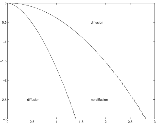
Figure 1: Boundaries of the portion of the no-diffusion region in $x\geq 0$ for linear flow $v(x)=x$, with $\lambda=1$, and $D=2$. The top boundary is $y=a(x)$ and the bottom is $y=b(x)$. The jagged lines for large $x$ are due to both the decreasing density of our stretched grid and plotting artifacts.

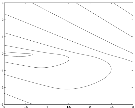
Figure 2: Contour plot of $\phi$ in $x\geq 0$ for linear flow $v(x)=x$, with $\lambda=1$ and $D=2$. The contours are at $\phi=3^{-n}$, for $n=1,2,\dots,7$, from around the origin outwards.

3.1 The nature of successful paths

A particle path that starts far from the origin, but hits the origin before being marked, has a distinctive shape which is observed in Monte-Carlo experiments. In its first wind about the origin the particle moves from the far field into the near-origin region. This motion is essentially ballistic, and is discussed further in §5. After arriving in the near-origin region the particle winds around the origin with large fluctuations, possibly making large excursions away from the origin. Eventually, the particle spirals into the origin in such a way that it never returns to the scale of a previous spiral, and each wind about the origin results in a huge decrease in the particle’s distance from the origin. This motion is discussed in §4. The probability of this direct spiralling motion increases as the particle gets closer to the origin.

Now, the probability of an unsuccessful wind, i.e. a wind that does not significantly reduce the distance of the particle from the origin, must be a rapidly decaying function of the winding number, so that there is a non-zero probability of hitting the origin before marking in the limit of infinite winding number. In particular, this implies that the near-origin problem cannot be governed solely by Brownian scaling, as this would give a constant (limiting) probability of failure on each wind. This tension against pure Brownian scaling characterizes the dynamics of the near-origin region, and leads to the curious scaling laws described below.

4 Near-field scaling law

Near the origin, the position of the diffusion-off boundary is controlled by the balance between the two effects that lead to failure of the directly spiralling motion: either the particle path is marked before it hits the origin, or the particle fails to continue spiralling and returns to the scale of its previous wind. Because the relative decrease in scale on each wind becomes greater and greater, the estimate of the balance of these two sources of failure can be made (asymptotically in small $x$, or large winding number) by considering just one half-wind.

Now consider one half-wind for a particle near the origin starting at a point $(x_{1},y_{1})$ on the diffusion-off boundary. We suppose that the flow $v(x)$ is antisymmetric, that $v(x)>0$ for $x>0$, and that $v(x)\simeq|x|^{\beta}$ for small $x$, where $A\simeq B$ means that $A/B$ is (at worst) a slowly varying function, which may be negative. In this case, the no-diffusion region lies in $xy\leq 0$. We assume that $y_{1}\simeq|x_{1}|^{\alpha}$, and we see that $x_{1}y_{1}<0$.

To obtain a consistent balance, we find that the dominant contribution to the probability of being marked on a half-wind comes from the motion in the no-diffusion region, and has probability $F_{1}\simeq y_{1}/v(x_{1})$, for sufficiently small $x_{1}$. For $v(x)\simeq|x|^{\beta}$, we find $F_{1}\simeq|x_{1}|^{\alpha-\beta}$.

Next, consider the particle motion from the diffusion-on boundary until it first hits the $y$ axis. From Brownian scaling, the particle first hits the $y$ axis at $y_{2}\simeq|x_{1}|^{\beta+2}$. Now the condition for the particle to continue to spiral into the origin is that it hits the diffusion-off boundary before it makes an excursion from the $y$ axis with $x$ displacement of scale $x_{1}$. Thus this type of failure has probability $F_{2}\simeq x_{2}/(|x_{1}|+|x_{2}|)\simeq x_{2}/x_{1}$, where $x_{2}$ is given by $y_{2}\simeq|x_{2}|^{\alpha}$, with $x_{2}y_{2}<0$. So $F_{2}\simeq|x_{1}|^{(\beta+2)/\alpha-1}$. The net probability of failure $F_{1}+F_{2}$ in this half-wind is a minimum when $F_{1}\simeq F_{2}$, which implies that the scaling exponents are equal, giving:

$$\alpha^{2}-\alpha(\beta-1)-(\beta+2)=0.$$ (10)

The scaling law thus has exponent

$$\alpha={\mbox{$\frac{1}{2}$}}(\beta-1+(\beta^{2}+2\beta+9)^{\frac{1}{2}}).$$ (11)

For the Kolmogorov diffusion, we therefore predict a scaling exponent $\alpha=\sqrt{3}$.

We attempted to determine the slowly varying function, or possibly constant, prefactor in the above scaling law, but were unable to adequately control the tails of some of the distributions we encountered (particularly in the $y$ direction).

Table 1 compares the scaling (11) with the results of the numerical solution of (7), in $-1\leq x\leq 1$ and $-1\leq y\leq 1$, with killing boundary conditions. We compute the numerical exponents by a least-squares fit of

$$\log(-b(x))=c+m\log x$$ (12)

to the diffusion-off boundary $b(x)$, where $c$ and $m$ are constants.

Table 1: Scaling exponents in the near field for various power-law flows.

$\beta$	exact $\alpha$	numerical $\alpha$
$1/2$	$(\sqrt{41}-1)/4\approx 1.351$	$1.372$
$1$	$\sqrt{3}\approx 1.732$	$1.760$
$3/2$	$(\sqrt{57}+1)/4\approx 2.137$	$2.201$
$2$	$(\sqrt{17}+1)/2\approx 2.562$	$2.568$

This leads us to the following conjecture.

Conjecture 1.

If $v(x)$ is antisymmetric, $v(x)>0$ for $x>0$, and

$$\lim_{x\downarrow 0}\frac{\log v(x)}{\log x}=\beta>0,$$ (13)

then the diffusion-off boundary $b(x)$ satisfies

$$\lim_{x\downarrow 0}\frac{\log(-b(x))}{\log x}={\mbox{$\frac{1}{2}$}}(\beta-1+(\beta^{2}+2\beta+9)^{\frac{1}{2}}).$$ (14)

Our numerical experiments do not exclude the possibility that if $v(x)\propto|x|^{\beta}$, then $b(x)\propto|x|^{\alpha}$, but this clearly cannot be shown definitively by numerical means.

If, instead of the independent exponential time used elsewhere, we use a spatially dependent marking rate $\lambda(x)\simeq|x|^{\Lambda}$ to limit the time, we can carry the same argument through to find

$$\alpha={\mbox{$\frac{1}{2}$}}(\beta-\Lambda-1+(\beta^{2}+2\beta+9+\Lambda^{2}-2\beta\Lambda+2\Lambda)^{1/2}),$$ (15)

although it is necessary to have $\beta>\Lambda$ to obtain a non-degenerate solution. Numerical studies also support this scaling exponent, but this has not been verified to as high an accuracy as the above conjecture.

5 WKB asymptotics in the far field

As in the near field, the far-field scaling is governed by a balance of rare events. Here, we balance the probability that the particle path remains unmarked with the probability that the path has a sufficient diffusive motion to move to $x=0$. If the particle takes a long time to move to $x=0$, we increase the probability of the purely diffusive motion, but we also increase the probability that the particle path is marked, and vice versa.

Throughout this section we assume that $v$ is antisymmetric, continuously differentiable, and that $v^{\prime}(x)>0$ for all $x$ (where the ^′ denotes a derivative). This ensures that the no-diffusion region is connected, and its boundaries are functions of $x$.

We derive the scaling of the most important regions of the far field by considering the $x$ and $y$ motion separately. First, we consider the motion in the $x$ direction. The probability density function for an unmarked Brownian particle in one dimension is

$$p(x,x_{0},t)\equiv(4\pi Dt)^{-1/2}\exp\left(-\frac{(x-x_{0})^{2}}{4Dt}-\lambda t\right),$$ (16)

and in the limit of large $x_{0}>0$, the dominant contribution of unmarked particles that hit $x=0$ is from paths of duration around $t_{0}$, given by

$$\frac{x_{0}^{2}}{4Dt_{0}}=\lambda t_{0},$$ (17)

balancing the probability of achieving the large diffusive stretch with the probability of remaining unmarked for a long time. (This implies a drift speed of $\sqrt{4\lambda D}$, which is exactly the drift of a Brownian motion conditioned on tending to infinity without being $\lambda$-marked.) If we now consider the advection in the $y$ direction with velocity scale $V$, we see that particles starting at $(x_{0},y_{0})$, where

$$y_{0}\simeq-Vt_{0}$$ (18)

will have both coordinates hit $0$ at roughly the same time. Thus particles starting in the neighbourhood of

$$y\simeq-Vx/(\lambda D)^{1/2}$$ (19)

make the largest contribution to the flux of unmarked particles to the origin. The no-diffusion region is close to this region of the plane, so that it can control particles in this dynamically significant region.

5.1 The meaning of ‘far field’

These ideas can be refined to give the full leading-order behaviour of the diffusion-off and diffusion-on boundaries in the far field. We suppose that $x$ scales as $X$, that the velocity scales as $V$, and that $y$ scales as $XV/(4\lambda D)^{1/2}$. Rescaling the backward equation (7) gives

$$\tilde{v}(\tilde{x}){\frac{\partial\phi}{\partial\tilde{y}}}+{\mbox{$\frac{1}{2}$}}\epsilon^{2}\left[{\frac{\partial^{2}\phi}{\partial\tilde{x}^{2}}}\right]^{+}-{\mbox{$\frac{1}{2}$}}\epsilon^{-2}\phi=0,$$ (20)

where tildes denote nondimensional quantities and $\epsilon^{2}\equiv(D/\lambda)^{1/2}X^{-1}$. We now drop the tildes, and work with the non-dimensionalized equation (20) for the remainder of §5. Next, we seek a solution of the form $\phi(x,y;\epsilon)=\exp(-S(x,y;\epsilon)/\epsilon^{2})$, and find that $S(x,y;\epsilon)$ satisfies the equation

$$-v(x){\frac{\partial S}{\partial y}}+{\mbox{$\frac{1}{2}$}}\left[\left({\frac{\partial S}{\partial x}}\right)^{2}-\epsilon^{2}{\frac{\partial^{2}S}{\partial x^{2}}}\right]^{+}={\mbox{$\frac{1}{2}$}},$$ (21)

on which we impose the boundary condition $S(0,0)=0$. We find the boundaries of the no-diffusion region $y=a(x)$ and $y=b(x)$ as asymptotic expansions in $\epsilon$, as $\epsilon\to 0$:

$$a(x) =a_{0}(x)+a_{1}(x)\epsilon+a_{2}(x)\epsilon^{2}+O(\epsilon^{3}),$$ (22)

$$b(x) =b_{0}(x)+b_{1}(x)\epsilon+b_{2}(x)\epsilon^{2}+O(\epsilon^{3}).$$

The expansion in $\epsilon$ is needed to split a double root.

In the diffusion regions, we seek a solution of (21) in WKB form:

$$S(x,y;\epsilon)\sim S_{0}(x,y)+S_{1}(x,y)\epsilon+S_{2}(x,y)\epsilon^{2}+\cdots.$$ (23)

Terms with odd powers of $\epsilon$ cannot be ruled out in region $3$ due to $\epsilon$-scale features in region $2$. Substituting (23) into (21) and expanding, we find the equations

$$-v(x){\frac{\partial S_{0}}{\partial y}}+{\mbox{$\frac{1}{2}$}}\left({\frac{\partial S_{0}}{\partial x}}\right)^{2} ={\mbox{$\frac{1}{2}$}},$$ (24)

$$-v(x){\frac{\partial S_{1}}{\partial y}}+{\frac{\partial S_{0}}{\partial x}}{\frac{\partial S_{1}}{\partial x}} =0,$$ (25)

$$-v(x){\frac{\partial S_{2}}{\partial y}}+{\frac{\partial S_{0}}{\partial x}}{\frac{\partial S_{2}}{\partial x}} ={\mbox{$\frac{1}{2}$}}{\frac{\partial^{2}S_{0}}{\partial x^{2}}}-{\mbox{$\frac{1}{2}$}}\left({\frac{\partial S_{1}}{\partial x}}\right)^{2}$$ (26)

at the first three orders.

As is standard (see, for instance [3] for more details), we solve the Hamilton–Jacobi equation (24) by casting it as its equivalent set of Hamiltonian ordinary differential equations. We first define a Hamiltonian

$$H(x,y,p_{x},p_{y})\equiv-v(x)p_{y}+{\mbox{$\frac{1}{2}$}}p_{x}^{2}$$ (27)

from (24), and observe that the characteristics of the Hamilton–Jacobi equation (24) satisfy the Hamilton equations

$${\frac{{\mathrm{d}}x}{{\mathrm{d}}\tau}} ={\frac{\partial H}{\partial p_{x}}}=p_{x},$$ (28)

$${\frac{{\mathrm{d}}y}{{\mathrm{d}}\tau}} ={\frac{\partial H}{\partial p_{y}}}=-v(x),$$

$${\frac{{\mathrm{d}}p_{x}}{{\mathrm{d}}\tau}} =-{\frac{\partial H}{\partial x}}=v^{\prime}(x)p_{y},$$

$${\frac{{\mathrm{d}}p_{y}}{{\mathrm{d}}\tau}} =-{\frac{\partial H}{\partial y}}=0,$$

where $x$, $y$, $p_{x}\equiv\partial{S_{0}}/\partial{x}$ and $p_{y}\equiv\partial{S_{0}}/\partial{y}$ are considered as functions of the ray time $\tau$. The direction of the ray time has been chosen to ensure that information propagates away from the origin, and is in the opposite direction to the time of particle motion. Terms such as diffusion-off boundary and diffusion-on boundary refer to the underlying particle motion, and not to the motion of rays. We then find that the change in $S_{0}$ along a ray from $(x_{s},y_{s})$ to $(x_{e},y_{e})$ is

$$\Delta S_{0}\equiv\int_{(x_{s},y_{s})}^{(x_{e},y_{e})}\left(p_{x}{\mathrm{d}}x+p_{y}{\mathrm{d}}y\right),$$ (29)

but that $S_{1}$ is constant on rays.

For a ray that remains in the diffusion regions, we introduce the quantity

$${\mathsf{S}}(x_{s},y_{s};x_{e},y_{e})\equiv\int_{(x_{s},y_{s})}^{(x_{e},y_{e})}\left(p_{x}{\mathrm{d}}x+p_{y}{\mathrm{d}}y\right),$$ (30)

where the integral is taken along the ray that runs from $(x_{s},y_{s})$ to $(x_{e},y_{e})$ with minimal $\Delta S_{0}$, so that that $S_{0}(x_{1},y_{1})={\mathsf{S}}(0,0;x_{1},y_{1})$ in region $1$. We note that

$${\frac{\partial{\mathsf{S}}}{\partial x_{e}}}(x_{s},y_{s};x_{e},y_{e}) =p_{x}(\tau_{e}),$$ (31)

$${\frac{\partial{\mathsf{S}}}{\partial y_{e}}}(x_{s},y_{s};x_{e},y_{e}) =p_{y}(\tau_{e}),$$

$${\frac{\partial{\mathsf{S}}}{\partial x_{s}}}(x_{s},y_{s};x_{e},y_{e}) =-p_{x}(\tau_{s}),$$

$${\frac{\partial{\mathsf{S}}}{\partial y_{s}}}(x_{s},y_{s};x_{e},y_{e}) =-p_{y}(\tau_{s}),$$

where $\tau_{s}$ and $\tau_{e}$ are the ray time at the start and end of the ray, respectively.

We extend the idea of rays to cover the no-diffusion region; here they have the Hamiltonian $-v(x)p_{y}={\mbox{$\frac{1}{2}$}}$, and we extend our definition of ${\mathsf{S}}$ with

$${\mathsf{S}}(x_{s},y_{s};x_{e},y_{e})=\frac{y_{s}-y_{e}}{2v(x_{s})},$$ (32)

where $(x_{s},y_{s})$ and $(x_{e},y_{e})$ are both in the no-diffusion region. Note that $x_{s}=x_{e}$ on a ray in the no-diffusion region. However, ${\mathsf{S}}$ notation is not used for pieces of ray that cross from a diffusion region to a no-diffusion region or vice versa.

5.2 Region 1

In region $1$, we see that

$$S_{0}(x,y) ={\mathsf{S}}(0,0;x,y),$$ (33)

$$S_{1}(x,y) =0,$$

and we fit the boundary between regions $1$ and $2$ by requiring

$$\left({\frac{\partial S}{\partial x}}\right)^{2}-\epsilon^{2}{\frac{\partial^{2}S}{\partial x^{2}}}=0$$ (34)

on this boundary. This condition gives

$${\frac{\partial S_{0}}{\partial x}}(x,a_{0}(x)+)=0,$$ (35)

where the trailing $+$ denotes a limit from above. This, not surprisingly, is also the condition for the action to be stationary under boundary perturbations. Using this condition, we see that

$$p_{x}=\left(1-v(x)/v(x_{0})\right)^{1/2}$$ (36)

on a ray that hits the diffusion-on boundary at $x=x_{0}$, and so

$$a_{0}(x)=-\int_{0}^{x}v(\xi)\left(1-\frac{v(\xi)}{v(x)}\right)^{-1/2}\,{\mathrm{d}}\xi.$$ (37)

Now we can also compute the first-order correction to the diffusion-on boundary. On the diffusion-on boundary, and working to $O(\epsilon^{2})$, the condition for the discriminant to change sign (34) implies

$$\left[{\frac{\partial^{2}S_{0}}{\partial x\partial y}}(x,a_{0}(x)+)a_{1}(x)\right]^{2}-{\frac{\partial^{2}S_{0}}{\partial x^{2}}}(x,a_{0}(x)+)=0.$$ (38)

Next, we calculate the second-order derivatives in (38). First, by differentiating (35), we see that

$${\frac{\partial^{2}S_{0}}{\partial x^{2}}}(x,a_{0}(x)+)+{\frac{\partial^{2}S_{0}}{\partial x\partial y}}(x,a_{0}(x)+)a_{0}^{\prime}(x)=0.$$ (39)

Since the rays are vertical just above the diffusion-on boundary ($p_{x}=0$, and $p_{y}=-(2v(x))^{-1}$), we compute $\partial^{2}S_{0}/\partial x\partial y$ just above the diffusion-on boundary by differentiating along rays:

$${\frac{\partial^{2}S_{0}}{\partial x\partial y}}(x,a_{0}(x)+)=\frac{{\mathrm{d}}p_{x}}{{\mathrm{d}}\tau}\left(\frac{{\mathrm{d}}y}{{\mathrm{d}}\tau}\right)^{-1}=-v^{\prime}(x)p_{y}/v(x)=-\left(\frac{1}{2v(x)}\right)^{\prime},$$ (40)

and so

$${\frac{\partial^{2}S_{0}}{\partial x^{2}}}(x,a_{0}(x)+)=a_{0}^{\prime}(x)\left(\frac{1}{2v(x)}\right)^{\prime}.$$ (41)

Now, we use the second derivatives (40, 41) in the perturbation discriminant (38) to find the first-order correction to the diffusion-on boundary:

$$a_{1}^{2}(x)={\frac{\partial^{2}S_{0}}{\partial x^{2}}}(x,a_{0}(x)+)\left({\frac{\partial^{2}S_{0}}{\partial x\partial y}}(x,a_{0}(x)+)\right)^{-2}=a_{0}^{\prime}(x)\left[\left(\frac{1}{2v(x)}\right)^{\prime}\right]^{-1}.$$ (42)

We choose the positive root of (42) to keep the discriminant positive in region $1$.

Projecting our asymptotic expansion for $a(x)$ into the class of decreasing functions, we obtain the approximation

$$\bar{a}(x)\equiv a_{0}(x)\left(1-\epsilon\frac{a_{1}(x)}{a_{0}(x)}\right)^{-1},$$ (43)

so that $a(x)-\bar{a}(x)=O(\epsilon^{2})$.

The action $S_{0}(x,a_{0}(x))$ is then

$$S_{0}(x,a_{0}(x))=-\int_{0}^{x}\frac{a_{0}^{\prime}(\xi)}{2v(\xi)}\,{\mathrm{d}}\xi.$$ (44)

We find, then, that for the power-law flow $v(x)=\operatorname{sgn}(x)|x|^{\beta}$, the first two terms in the asymptotic expansion of the diffusion-off boundary $a(x)$ in $x>0$ are

$$a_{0}(x) =-x^{\beta+1}B({\mbox{$\frac{1}{2}$}},1+\beta^{-1})/\beta$$ (45)

$$a_{1}(x) =x^{\beta+1/2}\left[2(\beta^{-1}+\beta^{-2})B({\mbox{$\frac{1}{2}$}},1+\beta^{-1})\right]^{1/2},$$

and, just for interest, that

$$S_{0}(x,a_{0}(x))=x(1+\beta^{-1})B({\mbox{$\frac{1}{2}$}},1+\beta^{-1})/2,$$ (46)

where $B$ is the Beta function.

5.3 Region 2

To find the boundary $b(x)$ of region $2$ we find the points at which the discriminant (34) is zero. The action in region $2$ is easily computed:

$$S(x,y) =S(x,a(x))+\frac{a(x)-y}{2v(x)}$$ (47)

$$=S_{0}(x,a_{0}(x))+\frac{a_{0}(x)-y}{2v(x)}+O(\epsilon^{2}).$$

Substituting (47) into the discriminant, we find $b_{0}=a_{0}$, and then at first order we find

$$b_{1}^{2}(x)=a_{0}^{\prime}(x)\left[\left(\frac{1}{2v(x)}\right)^{\prime}\right]^{-1}.$$ (48)

Here, we must choose the negative root to keep the discriminant negative in region $2$; we see that $b_{1}=-a_{1}$. We also see that (48) has a root that gives the perturbation to the diffusion-on boundary; this is reassuring, as it shows that the analysis in region $1$ is consistent with the analysis in region $2$. Note that the symmetry between the diffusion-off and diffusion-on boundaries about $y=a_{0}(x)$ is not expected to extend to $a_{2}$ and $b_{2}$.

5.4 Region 3

The main purpose of §5 is to determine the far-field approximations to the diffusion-off and diffusion-on boundaries, which can be done without reference to region $3$. However, there are still some interesting features of the field in region $3$, which are discussed here.

By direct calculation, with error $O(\epsilon^{2})$, the action in region $2$ is the analytic continuation of the action in region $1$. Hence, the action in region $3$ is, with error $O(\epsilon^{2})$, the analytic continuation of the action in region $1$. Now the ray tubes in region 2 are perturbed (in position and cross-section) by $O(\epsilon^{2})$ due to the lack of diffusion, and they spend only $O(\epsilon)$ ray time, $\tau$, in region $2$. This suggests that the true difference between the analytic continuation of the region $1$ solution to region $3$ and the true region $3$ solution could be as small as $O(\epsilon^{3})$.

The only remaining feature of region $3$ is its boundary $y=c(x)$ with region $1$. This boundary is a caustic of the Hamilton–Jacobi problem (24). In region $1$, optimum rays head straight away from the origin, moving straight into positive $x$, whereas in region $3$ optimum rays move into negative $x$ before looping back into positive $x$. There is a transition region in the neighbourhood of the boundary of regions $1$ and $3$ where non-optimal rays exist; these rays are plotted for linear flow ($v(x)=x$) in figure 3, in which we launch rays from the origin to a point just inside the boundary of region $1$. There are three rays from the origin to this point. Ray A first moves into $x<0$, and has a large loop there before reaching $x=0$. Ray B also moves into $x<0$, but only has a small tight loop there. Finally, ray C moves directly into $x>0$. Rays A and C give local minima of the action, but ray B gives a local maximum. By definition, the boundary $y=c(x)$ between regions $1$ and $3$ is the curve on which the actions of rays of type A and type C are equal. Although figure 3 only shows the behaviour of rays in linear flow, we believe the qualitative behaviour of these rays is generic.

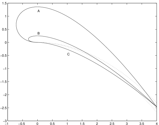
Figure 3: Rays from the origin to a point just inside region $1$, in linear flow (but ignoring the small effect from the no-diffusion region in $x<0$, $y>0$). The rays are plotted as solid lines, and the boundary between regions $1$ and $3$, and the line in region $1$ on which non-optimal rays appear, are plotted as dotted lines. The caustic appears when the action along ray A and ray C are equal. Ray B is a local maximum of the action.

For linear flow we explicitly determine the action in $x\geq 0$, and can therefore explicitly find this caustic. Define

$$S_{\pm}(x,y)\equiv\mbox{$\frac{2}{3}$}(x^{2}/\tau_{\pm}(x,y)+\tau_{\pm}(x,y))\pm\mbox{$\frac{1}{3}$}x$$ (49)

where

$$\tau_{\pm}(x,y)\equiv(x^{2}\pm 6y)^{1/2}\pm x,$$ (50)

and then $S(x,y)=S_{-}(x,y)+O(\epsilon^{2})$ in $y\leq c(x)$, and $S(x,y)=S_{+}(x,y)+O(\epsilon^{2})$ in $y\geq c(x)$. We find the caustic $y=c(x)$ by solving $S_{+}(x,y)=S_{-}(x,y)+O(\epsilon^{2})$, giving

$$c(x)=-x^{2}/(4\sqrt{3})+O(\epsilon^{2}).$$ (51)

5.5 Far-field discussion

Figure 4 plots the asymptotic results of §5 for the far-field diffusion-off and diffusion-on boundaries, and gives a comparison with the numerically computed boundaries, for the case of a linear flow. Despite the large asymptotic parameter ($\epsilon\approx 0.8$), there is very good agreement between the asymptotic approximation of the diffusion-off boundary and the numerical boundary. The fit of the diffusion-on boundary is worse, although there is still reasonable agreement between the leading-order approximation $a_{0}(x)$ and the numerical boundary, which is between $a_{0}(x)$ and its first correction $\bar{a}(x)$.

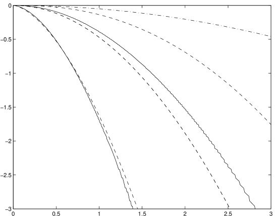
Figure 4: Comparison of numerical results and far-field asymptotics for the boundaries of the no-diffusion region, for linear flow $v(x)=x$, with $\lambda=1$, and $D=2$. From top to bottom, the numerical diffusion-on and diffusion-off boundaries are plotted with solid lines, and the dimensional forms of the curves $y=\bar{a}(x)$, $y=a_{0}(x)$ and our asymptotic approximation for $y=b(x)$ are plotted with dashed lines. The boundary, $y=c(x)$, between regions $1$ and $3$ is plotted with a dash-dotted line. The agreement between asymptotics and numerics is reasonable, given that $\epsilon\approx 0.8$, based on $X=2$.

This large deviation calculation may equivalently be done in terms of a path integral formulation of the problem, in which the ray equations (28) arise as the equations governing the classical path.

6 Variant problems

6.1 Exact snap to far-field asymptotics

Throughout this subsection, we assume that $v$ is antisymmetric, continuous, $v(x)>0$ for $x>0$, and without loss of generality that $\sup_{x}v(x)=1$. We further assume that there is a finite $x_{m}\equiv\inf\{x:v(x)=1\}$. Under a local ‘sharpness’ condition of $v$ in the neighbourhood of $x_{m}$ (given below), for sufficiently large $|y|$ the no-diffusion region degenerates to the lines $x=-\operatorname{sgn}(y)x_{m}$, on which the field decays exponentially in $|y|$. This is seen in figure 5, which shows this phenomenon with the flow field

$$v(x)=\begin{cases}x,&|x|<1\\ \operatorname{sgn}x,&\mbox{otherwise}.\end{cases}$$ (52)

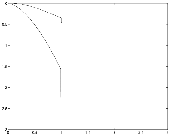
Figure 5: A no-diffusion region degenerating to a line, for $D=2$, $\lambda=1$, and with the flow field (52).

Based on our WKB analysis, we conjecture a necessary and sufficient condition for the no-diffusion region to degenerate to lines $x=-\operatorname{sgn}(y)x_{m}$ in sufficiently large $|y|$. We simply ask whether a ray from the origin hits $x=x_{m}$ with $p_{x}=0$ at a finite ray time (which is the condition for the ray to enter the no-diffusion region). This reduces to the condition

$$\int_{0}^{x_{m}}\left(1-\frac{v(x)}{v(x_{m})}\right)^{-1/2}{\mathrm{d}}x<\infty,$$ (53)

for the no-diffusion region to degenerate to a line, and not otherwise. Based on numerical tests the above condition also appears valid for the case of bounded $x$, with reflecting boundary conditions, although the WKB argument given above is not directly applicable because of caustics due to boundary reflections.

An example for which the above condition predicts no snap is $v(x)=\max(x(2-x),1)$ for $x\geq 0$, and this was numerically verified. This example is close to the marginal case.

In some systems, and in some regions of the plane, this snap of the no-diffusion region leads to a curious behaviour in which the field $\phi(x,y)$ agrees exactly with its leading-order far-field asymptotic solution, up to an undetermined multiplicative constant. We refer to this phenomenon as an exact snap.

We now consider this exact snap in detail. From (20), $\phi(x,y)\leq\exp(-{\mbox{$\frac{1}{2}$}}\epsilon^{-2}|y|)$ for all $(x,y)$, based on the maximum advection velocity. Define $y_{m}$ as the infimum of $|y|$ in the degenerate part of the no-diffusion region.

Define $\psi$ so that

$$\phi(x,y)\equiv\exp(-{\mbox{$\frac{1}{2}$}}\epsilon^{-2}|y|)\psi(x,y),$$ (54)

then equation 20 implies for $|y|>y_{m}$ that

$$v(x){\frac{\partial\psi}{\partial y}}+{\mbox{$\frac{1}{2}$}}\epsilon^{2}{\frac{\partial^{2}\psi}{\partial x^{2}}}-{\mbox{$\frac{1}{2}$}}\epsilon^{-2}(1+\operatorname{sgn}(y)v(x))\psi=0,$$ (55)

with discontinuities in $\partial\psi/\partial x$ at $x=\pm x_{m}$ in respectively $y<-y_{m}$ and $y>y_{m}$.

Under the above condition for a degenerate no-diffusion region, we find areas of the plane for which $\partial\psi/\partial y=0$, namely $y<-y_{m}$ and $x<x_{m}$, and the corresponding area in $y>0$. Equation (55) then simplifies, and we are able to find the field in these areas of the plane, up to an undetermined constant $\phi(x_{m},y_{m})$.

For $v(x)=\max(x,1)$, for $x\geq 0$, we see that $x_{m}=1$, and that our WKB condition (53) is satisfied. In our exact snap areas, (55) can be exactly solved in terms of Airy functions and exponentials.

We test the hypothesis that $\partial\psi/\partial y=0$ in $x\leq 1$ for sufficiently large $|y|$ by computing

$${\cal N}(\xi_{1},\xi_{2};y_{1},y_{2})\equiv\sup_{\xi_{1}\leq x\leq\xi_{2}}\frac{|\psi(x,y_{1})-\psi(x,y_{2})|}{\psi(x,y_{1})+\psi(x,y_{2})}.$$ (56)

For the data of figure 5, we find that ${\cal N}(-\infty,1;-5.50,-7.46)=5\times 10^{-4}$. (In figure 5, these dimensionless values of $y$ correspond to dimensional values of $-1.95$ and $-2.64$ respectively, based on $X=1$ and $V=1$. This gives $\epsilon^{4}=2$.) It is difficult to get stronger numerical evidence for this in a doubly infinite system; our stretched grid coarsens away from the origin, and we choose $y$ stations far enough from the ends of the grid to ensure that the field is reasonably well resolved. For the values of $y$ chosen here, the grid spacing in $y$ is approximately $0.06$. We find, from our numerical results, that the decay of the field along the filament of the no-diffusion region on $x=-\operatorname{sgn}(y)x_{m}$, $|y|>y_{m}$ is $\exp(-0.998\times{\mbox{$\frac{1}{2}$}}\epsilon^{-2}y)$. Note, however, that the correlation coefficient between the grid points $(x_{i})$ and $(\log\phi(x_{i},-5.50))$, in $x\leq-1$, is $1-10^{-8}$. (We work in $x\leq-1$ because, for this problem, the predicted $\psi$ field is particularly simple here.) The exponential $(C_{1}\exp(\sqrt{2}\epsilon^{-2}x_{i}))$ (where $C_{1}$ is a constant) is an excellent fit to the $\phi$ field on $x<-1$, $y=-5.50$. We also find that $C_{2}\exp(\sqrt{2}\epsilon^{-2}x+{\mbox{$\frac{1}{2}$}}\epsilon^{-2}y)$ (where $C_{2}$ is a constant) is a good fit to the $\phi$ field over the area $y<-y_{m}$, $x<-1$. However, the decay at fixed $y<-y_{m}$ of $\phi(x,y)$ in $x>1$ is (numerically) far from $\exp(-\sqrt{2}\epsilon^{-2}x)$, demonstrating that there is no exact snap in this area.

A more convincing demonstration of this exact snap occurs in systems with bounded $x$ and reflecting boundary conditions. In the corresponding system with $x\in[-1,1]$ and unbounded $y$, higher resolution in $y$ is possible, giving for example ${\cal N}(-1,1;-5.49,-6.62)$ $<10^{-11}$. Here, the no-diffusion region degenerates onto $x=-\operatorname{sgn}(y)$ for sufficiently large $|y|$, and we are able to accurately resolve this boundary.

The reason we believe that some systems have an exact snap is that this is the slowest decaying mode, so if the optimization can match to this solution it can do no better than this for larger $|y|$, given the amplitude of $\phi$ at the matching $y$ value. It appears that an exact snap does not occur in any area of the plane for which there exists a possible particle path to the $x$ axis that does not pass through the no-diffusion region.

6.2 Disconnected no-diffusion regions

In the WKB calculation of §5 we assume that $v$ is antisymmetric, continuously differentiable with $v^{\prime}(x)>0$, the last condition ensuring that the no-diffusion region is connected, significantly simplifying the calculation. If however we allow intervals $|x|\in(\xi,\eta)$ where $v^{\prime}(x)=0$, these lead to gaps in the no-diffusion region over a range which includes $(\xi,\eta)$.

An example for $v$ with

$$v^{\prime}(x)=\begin{cases}0,&|x|\in(0.75,0.85)\\ 1,&\mbox{otherwise}\end{cases}$$ (57)

is given in figure 6, clearly showing a gap in the no-diffusion region due to the interval in which $v$ is flat. Notice that the width of the gap in the no-diffusion region is larger than the width of the interval in which the velocity is flat, and this is a generic feature of such systems. Also generic is the filament of no-diffusion region that hangs down from the part of the no-diffusion region connected to the origin. This filament shortens as the gap size is reduced, and the $y$ value at which the filament ends always roughly matches the $y$ value at the bottom of the other side of the gap.

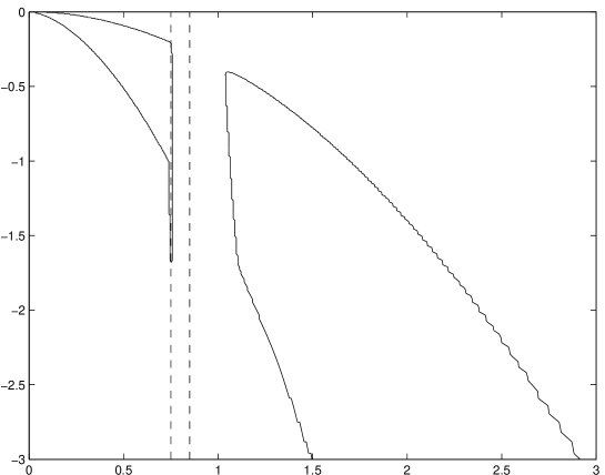
Figure 6: A gap in the no-diffusion region, for the flow field (57), with $D=2$ and $\lambda=1$. The dashed lines show the ends of the interval $(0.75,0.85)$ in which $v$ is constant.

If there are many such small gaps close together, the no-diffusion region is vertically striped, but its behaviour is almost the same as that of its envelope. This is because when a particle moves into the envelope, it either (i) enters a very $x$-restricted diffusion region which it passes through, (ii) enters a very $x$-restricted diffusion region and later hits the adjacent no-diffusion region, or (iii) goes straight into the no-diffusion region. In all cases, the particle leaves the envelope with almost the same $x$.

An extreme example of a striped envelope is when, apart from in the neighbourhood of the origin needed for success, the velocity is piecewise constant. In this case the no-diffusion strips are of zero width.

7 Discussion

We are now in a position to clearly describe the behaviour of a particle that ultimately hits the origin before its path is $\lambda$-marked. For definiteness, we consider a particle in the unbounded shear flow $v(x)=x$, started at $(0,y_{0})$ with $y_{0}<0$ and well into the far field. The particle first moves out into large $x>0$, to increase its flow speed towards the $x$ axis. When the particle reaches $y=y_{0}/2$ it turns around, and heads back towards $x=0$. Near this maximum of $x$, the particle gains a small advantage by turning diffusion off, and hence truncating a quadratic maximum in the $x$ motion, as seen in §5. The far-field motion (in the WKB limit) is little affected by the no-diffusion region, with corrections to the rays and the action first appearing at $O(\epsilon^{2})$ (and possibly higher), whereas the no-diffusion boundaries have corrections that scale as $\epsilon$, caused by the splitting of a double root. The structure of the no-diffusion region for $\epsilon=1$ is very similar to its structure in the far-field limit (i.e. small $\epsilon$).

When the particle finally arrives near $x=0$, it winds around the origin, with large fluctuations, until eventually it spirals directly into the origin. Controlling this rapid spiralling motion fixes the behaviour of the diffusion-off boundary near the origin, as seen in §4. In the near field the no-diffusion region is essential, as without it the probability of hitting the origin is zero. The near-field scaling laws are supported well by numerical experiments (including cases with power-law killing). A natural question is whether such scaling laws are possible for higher-order iterated diffusions, and whether it is possible to go beyond scaling laws to asymptotic expansions in the near field.

The no-diffusion region is intrinsically governed by a balance between the probability that the particle path is marked, and the probability that a particle hits the origin at all. Considering the optimum no-diffusion region as a function of $\lambda$, we see that as $\lambda$ increases, the probability of a particle starting at a fixed point hitting the origin marked or unmarked decreases.

The natural fluid-dynamical extension of this work is to optimal coupling in a linear flow. The separation $X$ between the two particles is governed by the Itô SDE

$${\mathrm{d}}X_{t}=A\cdot X_{t}\,{\mathrm{d}}t+(I-R(X_{t}))\cdot{\mathrm{d}}B_{t},$$ (58)

where $B$ is Brownian motion, $A$ is a traceless constant matrix, $I$ is the identity matrix, and $R$ is an orthogonal matrix. For each point, $x$, we choose $R(x)$ in order to rapidly shepherd $X$ into the origin, and hence achieve rapid coupling. We do this by forming the backward equation for the probability of successful coupling, analogous to (7). The local optimization problem, in this paper only a discrete choice, now becomes a continuum optimization problem, which may be solved by singular value decomposition [4]. The far field is still governed by ray theory, and similar techniques to those of §5 will still apply. However, the region corresponding to the no-diffusion region of this paper will have more structure, because the optimization is no longer a discrete choice. It may be possible to produce systems of the form (58) in which there is an intermediate scale resembling the near-field limit of §4. However, it is not clear if this effect will be important in real fluid-dynamical applications.

References

- [1] Gérard Ben Arous, Michael Cranston and Wilfrid S. Kendall, ‘Coupling constructions for hypoelliptic diffusions: two examples.’ ‘Stochastic analysis (Ithaca, NY, 1993),’ (Amer. Math. Soc., Providence, RI, 1995), vol. 57 of Proc. Sympos. Pure Math. pp. 193–212, pp. 193–212.
- [2] Richard Durrett, Probability: theory and examples (Duxbury Press, Belmont, CA, 1996), 2nd edn. ISBN 0-534-24318-5.
- [3] H. Goldstein, Classical Mechanics (Addison-Wesley, 1980), 2nd edn.
- [4] Kalvis M. Jansons and Paul D. Metcalfe, ‘Numerically optimized Markovian coupling and mixing in one-dimensional maps.’ preprint .
- [5] Wilfrid S. Kendall and Catherine J. Price, ‘Coupling iterated Kolmogorov diffusions.’ Electron. J. Probab. 9 (2004) 382–410.
- [6] A. Kolmogoroff, ‘Zufällige Bewegungen (zur Theorie der Brownschen Bewegung).’ Ann. Math. 35 (1934) 116–117.
- [7] Robert I. McLachlan and G. Reinout W. Quispel, ‘Splitting methods.’ Acta Numer. 11 (2002) 341–434.