A data-reconstructed fractional volatility model

Abstract

Based on criteria of mathematical simplicity and consistency with empirical market data, a stochastic volatility model is constructed, the volatility process being driven by fractional noise. Price return statistics and asymptotic behavior are derived from the model and compared with data. Deviations from Black-Scholes and a new option pricing formula are also obtained.

Keywords: Fractional noise, Induced volatility, Statistics of returns, Option pricing

1 Introduction

Classical Mathematical Finance has, for a long time, been based on the assumption that the price process of market securities may be approximated by geometric Brownian motion

$$\begin{array}[]{lll}dS_{t}&=&\mu S_{t}dt+\sigma S_{t}dB\left(t\right)\end{array}$$ (1)

In liquid markets the autocorrelation of price changes decays to negligible values in a few minutes, consistent with the absence of long term statistical arbitrage. Geometric Brownian motion models this lack of memory, although it does not reproduce the empirical leptokurtosis. On the other hand, nonlinear functions of the returns exhibit significant positive autocorrelation. For example, there is volatility clustering, with large returns expected to be followed by large returns and small returns by small returns (of either sign). This, together with the fact that autocorrelations of volatility measures decline very slowly[1] [2] [3], has the clear implication that long memory effects should somehow be represented in the process and this is not included in the geometric Brownian motion hypothesis.

One other hand, as pointed out by Engle[4], when the future is uncertain investors are less likely to invest. Therefore uncertainty (volatility) would have to be changing over time. The conclusion is that a dynamical model for volatility is needed and $\sigma$ in Eq.(1), rather than being a constant, becomes a process by itself. This idea led to many deterministic and stochastic models for the volatility ([5] [6] and references therein).

Using, at each step, both a criteria of mathematical simplicity and consistency with market data, a stochastic volatility model is constructed here, with volatility driven by fractional noise. It appears to be the minimal model consistent both with mathematical simplicity and the market data. It turns out that this data-inspired model is different from the many stochastic volatility models that have been proposed in the literature. The model will be used to compute the price return statistics and asymptotic behavior, which are compared with actual data. Deviations from the classical Black-Scholes result and a new option pricing formula are also obtained.

2 The induced volatility process

The basic hypothesis for the model construction are:

(H1) The log-price process $\log S_{t}$ belongs to a probability product space $\Omega\otimes\Omega^{{}^{\prime}}$ of which the first one, $\Omega$, is the Wiener space and the second, $\Omega^{{}^{\prime}}$, is a probability space to be characterized later on. Denote by $\omega\in\Omega$ and $\omega^{{}^{\prime}}\in\Omega^{{}^{\prime}}$ the elements (sample paths) in $\Omega$ and $\Omega^{{}^{\prime}}$ and by $\mathcal{F}_{t}$ and $\mathcal{F}_{t}^{{}^{\prime}}$ the $\sigma-$algebras in $\Omega$ and $\Omega^{{}^{\prime}}$ generated by the processes up to $t$. Then, a particular realization of the log-price process is denoted

$$\log S_{t}\left(\omega,\omega^{{}^{\prime}}\right)$$

This first hypothesis is really not limitative. Even if none of the non-trivial stochastic features of the log-price were to be captured by Brownian motion, that would simply mean that $S_{t}$ is a trivial function in $\Omega$.

(H2) The second hypothesis is stronger, although natural. We will assume that for each fixed $\omega^{{}^{\prime}}$, $\log S_{t}\left(\bullet,\omega^{{}^{\prime}}\right)$ is a square integrable random variable in $\Omega$.

———

From the second hypothesis it follows that, for each fixed $\omega^{{}^{\prime}}$,

$$\begin{array}[]{lll}\frac{dS_{t}}{S_{t}}\left(\bullet,\omega^{{}^{\prime}}\right)&=&\mu_{t}\left(\bullet,\omega^{{}^{\prime}}\right)dt+\sigma_{t}\left(\bullet,\omega^{{}^{\prime}}\right)dB\left(t\right)\end{array}$$ (2)

where $\mu_{t}\left(\bullet,\omega^{{}^{\prime}}\right)$ and $\sigma_{t}\left(\bullet,\omega^{{}^{\prime}}\right)$ are well-defined processes in $\Omega$. (Theorem 1.1.3 in Ref.[7])

Recall that if $\left\{X_{t},\mathcal{F}_{t}\right\}$ is a process such that

$$\begin{array}[]{lll}dX_{t}&=&\mu_{t}dt+\sigma_{t}dB\left(t\right)\end{array}$$ (3)

with $\mu_{t}$ and $\sigma_{t}$ being $\mathcal{F}_{t}-$adapted processes, then

$$\begin{array}[]{lll}\mu_{t}&=&\underset{\varepsilon\rightarrow 0}{\lim}\frac{1}{\varepsilon}\left\{\left.E\left(X_{t+\varepsilon}-X_{t}\right)\right|\mathcal{F}_{t}\right\}\\ \sigma_{t}^{2}&=&\underset{\varepsilon\rightarrow 0}{\lim}\frac{1}{\varepsilon}\left\{\left.E\left(X_{t+\varepsilon}-X_{t}\right)^{2}\right|\mathcal{F}_{t}\right\}\end{array}$$ (4)

The process associated to the probability space $\Omega^{{}^{\prime}}$ is now to be inferred from the data. According to (4), for each fixed $\omega^{{}^{\prime}}$ realization in $\Omega^{{}^{\prime}}$ one has

$$\sigma_{t}^{2}\left(\bullet,\omega^{{}^{\prime}}\right)=\underset{\varepsilon\rightarrow 0}{\lim}\frac{1}{\varepsilon}\left\{E\left(\log S_{t+\varepsilon}-\log S_{t}\right)^{2}\right\}$$ (5)

Each set of market data corresponds to a particular realization $\omega^{{}^{\prime}}$. Therefore, assuming the realization to be typical, the $\sigma_{t}^{2}$ process may be reconstructed from the data by the use of (5). To this data-reconstructed $\sigma_{t}$ process we call the induced volatility.

For practical purposes we cannot strictly use Eq.(5) to reconstruct the induced volatility process, because when the time interval $\varepsilon$ is very small the empirical evaluation of the variance becomes unreliable. Instead, we estimate $\sigma_{t}$ from

$$\sigma_{t}^{2}=\frac{1}{\left|T_{0}-T_{1}\right|}\mathnormal{var}\left(\log S_{t}\right)$$ (6)

with a time window $\left|T_{0}-T_{1}\right|$ sufficiently small to give a reasonably local characterization of the volatility, but also sufficiently large to allow for a reliable estimate of the local variance of $\log S_{t}$.

As an example, daily data has been used with time windows of 5 to 9 days. The upper left panel of Fig.1 shows the result of application of (6) to the New York Stock Exchange (NYSE) aggregate index in the period 1966$-$2000, with a time window $\left|T_{0}-T_{1}\right|=5$ days. Notice that to discount trend effects and approach asymptotic stationarity of the process, before application of (6), the data has been detrended and rescaled as explained in Ref.[8]. Namely, a polynomial fit is performed for increasing orders until the fitted polynomial is no longer well conditioned. This seems to be a reasonable detrending method insofar as it leads to an asymptotically stationary signal [8].

Then, as a first step towards finding a mathematical characterization of the induced volatility process one looks for scaling properties. Namely one checks whether a relation of the form

$$E\left|\sigma\left(t+\Delta\right)-\sigma\left(t\right)\right|\sim\Delta^{H}$$ (7)

or

$$E\left|\frac{\sigma\left(t+\Delta\right)-\sigma\left(t\right)}{\sigma\left(t\right)}\right|\sim\Delta^{H}$$ (8)

holds for the induced volatility process. This would be the behavior implied by most stochastic volatility models proposed in the past. It turns out that the data shows this to be a very bad hypothesis, meaning that the induced volatility process itself is not self-similar.

Instead, using a standard technique to detect long-range dependencies[9], one computes the empirical integrated log-volatility and finds that it is well represented by a relation of the form

$$\sum_{n=0}^{t/\delta}\log\sigma\left(n\delta\right)=\beta t+R_{\sigma}\left(t\right)$$ (9)

where, as shown in the lower right panel of Fig.1, the $R_{\sigma}\left(t\right)$ process has very accurate self-similar properties ($\delta=1$ day for daily data).

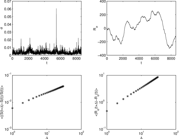
Figure 1: Self-similar properties of the integrated log-volatility $\beta t+R_{\sigma}\left(t\right)$ process

This suggests the following mathematical identification:

(a) Recall that if a nondegenerate process $X_{t}$ has finite variance, stationary increments and is self-similar

$$\mathnormal{Law}\left(X_{at}\right)=\mathnormal{Law}\left(a^{H}X_{t}\right)$$ (10)

then [10] $0<H\leq 1$ and

$$\mathnormal{Cov}\left(X_{s},X_{t}\right)=\frac{1}{2}\left(\left|s\right|^{2H}+\left|t\right|^{2H}-\left|s-t\right|^{2H}\right)E\left(X_{1}^{2}\right)$$ (11)

The simplest process with these properties is a Gaussian process called fractional Brownian motion. Fractional Brownian motion [11]

$$\mathbb{E}\left[B_{H}\left(t\right)\right]=0\qquad\mathbb{E}\left[B_{H}\left(t\right)B_{H}\left(s\right)\right]=\frac{1}{2}\left\{\left|t\right|^{2H}+\left|s\right|^{2H}-\left|t-s\right|^{2H}\right\}$$ (12)

has, for $H>\frac{1}{2}$ , a long range dependence

$$\sum_{n=1}^{\infty}\mathnormal{Cov}\left(B_{H}\left(1\right),B_{H}\left(n+1\right)-B_{H}\left(n\right)\right)=\infty$$ (13)

(b) Therefore, mathematical simplicity suggests the identification of the $R_{\sigma}\left(t\right)$ process with fractional Brownian motion.

$$R_{\sigma}\left(t\right)=kB_{H}\left(t\right)$$ (14)

From the data one obtains the Hurst coefficient $H\simeq 0.8$ (for the NYSE index). The same parametrization holds for the data of all individual companies that were tested, with $H$ in the range $0.8-0.9$.

For comparison the plot in the down left panel of Fig.1 shows the scaling test for the (NYSE) price process where, unlike the $R_{\sigma}\left(t\right)$ process, clear deviations are seen on the first few days.

From (9) and the identification (14) one concludes that the induced volatility may be modeled by

$$\log\sigma_{t}=\beta+\frac{k}{\delta}\left(B_{H}\left(t\right)-B_{H}\left(t-\delta\right)\right)$$ (15)

$\delta$ being the observation time scale (one day, for daily data). It means that the volatility is not driven by fractional Brownian motion but by fractional noise. For the volatility (at resolution $\delta$)

$$\sigma\left(t\right)=\theta e^{\frac{k}{\delta}\left\{B_{H}\left(t\right)-B_{H}\left(t-\delta\right)\right\}-\frac{1}{2}\left(\frac{k}{\delta}\right)^{2}\delta^{2H}}$$ (16)

the term $-\frac{1}{2}\left(\frac{k}{\delta}\right)^{2}\delta^{2H}$ being included to insure that $E\left(\sigma\left(t\right)\right)=\theta$.

Eqs. (2) and (15) define a stochastic volatility model.

$$\begin{array}[]{lll}dS_{t}&=&\mu S_{t}dt+\sigma_{t}S_{t}dB\left(t\right)\\ \log\sigma_{t}&=&\beta+\frac{k}{\delta}\left\{B_{H}\left(t\right)-B_{H}\left(t-\delta\right)\right\}\end{array}$$ (17)

In this coupled stochastic system, in addition to a mean value, volatility is driven by fractional noise. Notice that this empirically based model is different from the usual stochastic volatility models which assume the volatility to follow an arithmetic or geometric Brownian process. Also in the Comte and Renault model[12], it is fractional Brownian motion that drives the volatility, not its derivative (fractional noise). $\delta$ is the observation scale of the process. In the $\delta\rightarrow 0$ limit the driving process would be the distribution-valued process $W_{H}$

$$W_{H}=\lim_{\delta\rightarrow 0}\frac{1}{\delta}\left(B_{H}\left(t\right)-B_{H}\left(t-\delta\right)\right)$$ (18)

In (17) the constant $k$ measures the strength of the volatility randomness. Although phenomenologically grounded and mathematically well specified, the stochastic system (17) is still a limited model because, in particular, the fact that the volatility is not correlated with the price process excludes the modeling of leverage effects. It would be simple to introduce, by hand, such a correlation in the second equation in (17). However we do prefer not to do so at this time, because have not yet found a natural way to do it, which is as clear-cut and imposed by the data as the approach that led to (17).

3 The statistics of price returns

Here one computes the probability distribution of price returns implied by the stochastic volatility model (17). From (15) one concludes that $\log\sigma_{t}$ is a Gaussian process with mean $\beta$ and covariance

$$\psi\left(s,u\right)=\frac{k^{2}}{2\delta^{2}}\left\{\left|s-u+\delta\right|^{2H}+\left|u-s+\delta\right|^{2H}-2\left|s-u\right|^{2H}\right\}$$ (19)

This Gaussian process has non-trivial correlation for $H\neq\frac{1}{2}$. At each fixed time $\log\sigma_{t}$ is a Gaussian random variable with mean $\beta$ and variance $k^{2}\delta^{2H-2}$. Then,

$$p_{\delta}\left(\sigma\right)=\frac{1}{\sigma}p_{\delta}\left(\log\sigma\right)=\frac{1}{\sqrt{2\pi}\sigma k\delta^{H-1}}\exp\left\{-\frac{\left(\log\sigma-\beta\right)^{2}}{2k^{2}\delta^{2H-2}}\right\}$$ (20)

therefore

$$P_{\delta}\left(\log\frac{S_{T}}{S_{t}}\right)=\int_{0}^{\infty}d\sigma p_{\delta}\left(\sigma\right)p_{\sigma}\left(\log\frac{S_{T}}{S_{t}}\right)$$ (21)

with

$$p_{\sigma}\left(\log\frac{S_{T}}{S_{t}}\right)=\frac{1}{\sqrt{2\pi\sigma^{2}\left(T-t\right)}}\exp\left\{-\frac{\left(\log\left(\frac{S_{T}}{S_{t}}\right)-\left(\mu-\frac{\sigma^{2}}{2}\right)\left(T-t\right)\right)^{2}}{2\sigma^{2}\left(T-t\right)}\right\}$$ (22)

One sees that the effective probability distribution of the returns might depend both on the time lag $\Delta=T-t$ and on the observation time scale $\delta$ used to construct the volatility process. That this latter dependence might actually be very weak, seems to be implied by some surprising experimental results.

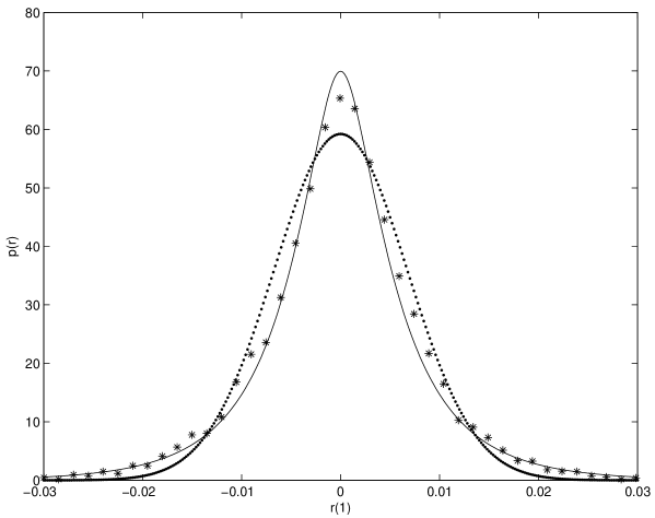
Figure 2: One-day NYSE returns compared with the model predictions and the lognormal

Before obtaining a closed form expression for $P_{\sigma}\left(\log\frac{S_{T}}{S_{t}}\right)$ and its asymptotic behavior, we will present some comparisons with market data. For the Fig.2 the same NYSE one-day data as before is used to fix the parameters of the volatility process. Then, using $H=0.83,$ $k=0.59,$ $\beta=-5,$ $\delta=1$, the one-day return distribution predicted by the model is compared with the data. The agreement is quite reasonable. For comparison a log-normal with the same mean and variance is also plotted in Fig.2. Then, in Fig. 3, using the same parameters, the same comparison is made for the $\Delta=1$ and $\Delta=10$ data.

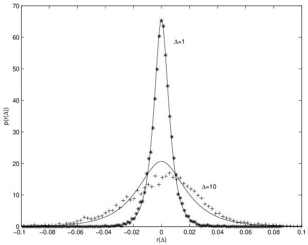
Figure 3: One and ten-days NYSE returns compared with the model predictions

Figure 4: One-minute USD-Euro returns compared with the model predictions, with parameters obtained from one-day NYSE data

Fig. 4 shows a somewhat surprising result. Using the same parameters and just changing $\Delta$ from $1$ (one day) to $\Delta=\frac{1}{440}$ (one minute), the prediction of the model is compared with one-minute data of USDollar-Euro market for a couple of months in 2001. The result is surprising, because one would not expect the volatility parametrization to carry over to such a different time scale and also because one is dealing with different markets. A systematic analysis of high-frequency data is now being carried out to test the degree of time-scale dependence of the volatility parametrization and its universality over different markets.

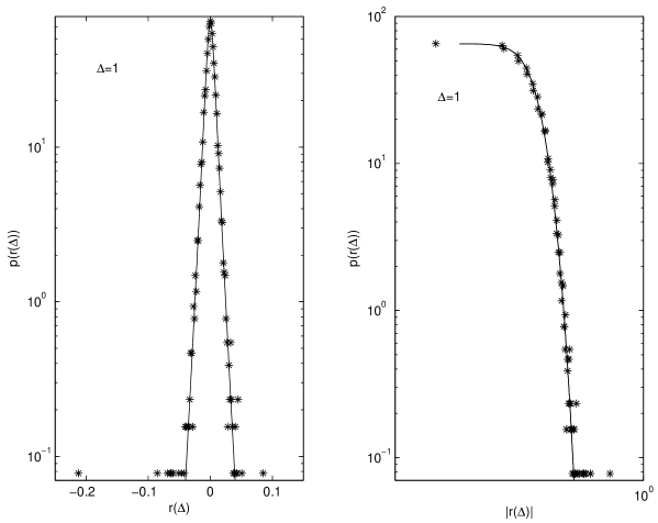
Figure 5: Semilogarithmic and loglog plots of NYSE data

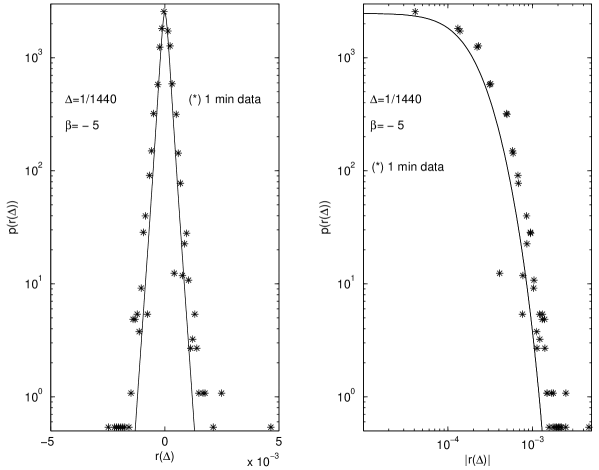
Figure 6: Semilogarithmic and loglog plots of USD-Euro data

In Fig.5 and Fig.6 we have displayed the same one-day and one-minute return data discussed before as well as the predictions of the model both in semilogarithmic and loglog plots.

Now we will establish a closed-form expression for the returns distribution and its asymptotic behavior. Using (20) and (22) in (21) and changing variables one obtains

$$P_{\delta}\left(r\left(\Delta\right)\right)=\frac{1}{4\pi\theta k\delta^{H-1}\sqrt{\Delta}}\int_{0}^{\infty}dxx^{-\frac{1}{2}}e^{-\frac{1}{C}\left(\log x\right)^{2}}e^{-\lambda x}$$ (23)

with

$$r\left(\Delta\right)=\log S_{T}-\log S_{t}\;,\;\theta=e^{\beta}\;,\;\Delta=T-t\;,\;\lambda=\frac{\left(r\left(\Delta\right)-r_{0}\right)^{2}}{2\Delta\theta^{2}}$$ (24)

and

$$r_{0}=\left(\mu-\frac{\sigma^{2}}{2}\right)\left(T-t\right)\;,\;C=8k^{2}\delta^{2H-2}$$ (25)

Expanding the exponential in (23)

$$4\pi\theta k\delta^{H-1}\sqrt{\Delta}P_{\delta}\left(r\left(\Delta\right)\right) = \sum_{n=0}^{\infty}\frac{1}{n!}\left(-\frac{1}{C}\right)^{n}\int_{0}^{\infty}dxx^{-\frac{1}{2}}e^{-\lambda x}\left(\log x\right)^{2n}$$ (26)

$$= \sum_{n=0}^{\infty}\frac{1}{n!}\left(-\frac{1}{C}\right)^{n}\frac{\partial^{2n}}{\partial z^{2n}}\left.\left(\lambda^{-z}\Gamma\left(z\right)\right)\right|_{z=\frac{1}{2}}$$

Finally

$$P_{\delta}\left(r\left(\Delta\right)\right)=\frac{1}{4\pi\theta k\delta^{H-1}\sqrt{\Delta}}\frac{1}{\sqrt{\lambda}}\left.\left(e^{-\frac{1}{C}\left(\log\lambda-\frac{d}{dz}\right)^{2}}\Gamma\left(z\right)\right)\right|_{z=\frac{1}{2}}$$ (27)

with asymptotic behavior, for large returns

$$P_{\delta}\left(r\left(\Delta\right)\right)\sim\frac{1}{\sqrt{\Delta\lambda}}e^{-\frac{1}{C}\log^{2}\lambda}$$ (28)

On the other hand, as seen from Figs. 5 and 6, the exact result (23) or (27) resembles the double exponential distribution recognized by Silva, Prange and Yakovenko[13] as a new stylized fact in market data. The double exponential distribution has been shown, by Dragulescu and Yakovenko[14], to follow from Heston’s [15] stochastic volatility model. Notice however that our model is different from Heston’s model in that volatility is driven by a process with memory (fractional noise). As a result, despite the qualitative similarity of behavior at intermediate return ranges, the analytic form of the distribution and the asymptotic behavior are different.

4 Option pricing

Assuming risk neutrality [16], the value $V\left(S_{t},\sigma_{t},t\right)$ of an option is the present value of the expected terminal value discounted at the risk-free rate

$$V\left(S_{t},\sigma_{t},t\right)=e^{-r\left(T-t\right)}\int V\left(S_{T},\sigma_{T},T\right)p\left(S_{T}|S_{t},\sigma_{t}\right)dS_{T}$$ (29)

$V\left(S_{T},\sigma_{T},T\right)=\max\left[0,S-K\right]$ and the conditional probability for the terminal price depends on $S_{t}$ and $\sigma_{t}$. $K$ is the strike price, $T$ the maturity time and $S_{t}$ and $\sigma_{t}$ the price and volatility of the underlying security.

Whenever the drift of a financial time series can be replaced by the risk-free rate we are in a risk-neutral situation. In stochastic volatility models (with or without fractional noise) this is not an accurate assumption. Nevertheless we will make use of (29) to obtain an approximate estimate of the deviations from Black-Scholes implied by the stochastic differential model (17). As in Hull and White [17], we make use of the relation between conditional probabilities of related variables, namely

$$p\left(S_{T}|S_{t},\sigma_{t}\right)=\int p\left(S_{T}|S_{t},\overline{\log\sigma}\right)p\left(\overline{\log\sigma}|\log\sigma_{t}\right)d\left(\overline{\log\sigma}\right)$$ (30)

$\overline{\log\sigma}$ being the random variable

$$\overline{\log\sigma}=\frac{1}{T-t}\int_{t}^{T}\log\sigma_{s}ds$$ (31)

that is, $\overline{\log\sigma}$ is the mean volatility from time $t$ to the maturity time $T$ conditioned to an average value $\log\sigma_{t}$ at time $t$. Then Eq.(29) becomes

$$V\left(S_{t},\sigma_{t},t\right)=\int C\left(S_{t},e^{\overline{\log\sigma}},t\right)p\left(\overline{\log\sigma}|\log\sigma_{t}\right)d\left(\overline{\log\sigma}\right)$$ (32)

$$C\left(S_{t},e^{\overline{\log\sigma}},t\right)=\int e^{-r\left(T-t\right)}V\left(S_{T},\sigma_{T},T\right)p\left(S_{T}|S_{t},\overline{\log\sigma}\right)dS_{T}$$ (33)

$C\left(S_{t},e^{\overline{\log\sigma}},t\right)$ being the Black-Scholes price for an option with average volatility $e^{\overline{\log\sigma}}$, which is known to be [18] [19]

$$C\left(S_{t},\sigma,t\right)=S_{t}\left(a+b\right)N\left(a,b\right)-Ke^{-r\left(T-t\right)}\left(a-b\right)N\left(a,-b\right)$$ (34)

with

$$\begin{array}[]{lll}a&=&\frac{1}{\sigma}\left(\frac{\log\frac{S_{t}}{K}}{\sqrt{T-t}}+r\sqrt{T-t}\right)\\ b&=&\frac{\sigma}{2}\sqrt{T-t}\end{array}$$ (35)

and

$$N\left(a,b\right)=\frac{1}{\sqrt{2\pi}}\int_{-1}^{\infty}dye^{-\frac{y^{2}}{2}\left(a+b\right)^{2}}$$ (36)

In a stochastic volatility model with fractional noise, instead of $V\left(S_{t},\sigma_{t},t\right)$, it would be more correct to write $V\left(S_{t},\sigma_{\leq t},t\right)$ to emphasize the dependence on the past. For simplicity we have used the first notation, with the provision that at no point, in the calculation below, Markov properties of the processes should be assumed, only their Gaussian nature.

To compute the conditional probability $p\left(\overline{\log\sigma}|\log\sigma_{t}\right)$ it follows from (17) that the process $\overline{\log\sigma}$ conditioned to $\log\sigma_{t}$ at $t$ is

$$\overline{\log\sigma}=\log\sigma_{t}+\frac{1}{T-t}\int_{t}^{T}\frac{k}{\delta}ds\int_{t}^{s}\left(dB_{H}\left(\tau\right)-dB_{H}\left(\tau-\delta\right)\right)$$ (37)

Notice that, because we want to compute the conditional probability of $\overline{\log\sigma}$ given $\log\sigma_{t}$ at time $t$, $\sigma_{t}$ in Eq.(37) is not a process but simply the value of the argument in the $V\left(S_{t},\sigma_{t},t\right)$ function.

As a $t-$dependent process the double integral in (37) is a centered Gaussian process. Therefore, given $\log\sigma_{t}$ at time $t$, $\overline{\log\sigma}$ is a Gaussian variable with conditional mean and variance

$$E\left\{\overline{\log\sigma}|\log\sigma_{t}\right\}=\log\sigma_{t}$$ (38)

$$\alpha^{2} = E\left\{\left(\overline{\log\sigma}-\log\sigma_{t}\right)^{2}|\log\sigma_{t}\right\}$$ (39)

$$= \frac{k^{2}}{\delta^{2}\left(T-t\right)^{2}}E\left\{\int_{t}^{T}ds\int_{t}^{s}\left[dB_{H}\left(\tau\right)-dB_{H}\left(\tau-\delta\right)\right]\int_{t}^{T}ds^{{}^{\prime}}\int_{t}^{s^{{}^{\prime}}}\left[dB_{H}\left(\tau^{{}^{\prime}}\right)-dB_{H}\left(\tau^{{}^{\prime}}-\delta\right)\right]\right\}$$

Expanding $\int_{t}^{s}\left[dB_{H}\left(\tau\right)-dB_{H}\left(\tau-\delta\right)\right]=B_{H}\left(s\right)-B_{H}\left(t\right)-B_{H}\left(s-\delta\right)+B_{H}\left(t-\delta\right)$ and using (12) one obtains

$$\alpha^{2}=\frac{k^{2}}{\delta^{2}\left(T-t\right)}\left\{\frac{1}{2\left(T-t\right)}I_{1}+I_{2}\right\}+k^{2}\delta^{2H-2}$$ (40)

with

$$I_{1}=\frac{2}{\left(2H+1\right)\left(2H+2\right)}\left\{\left(T-t+\delta\right)^{2H+2}+\left(T-t-\delta\right)^{2H+2}-2\left(T-t\right)^{2H+2}-2\delta^{2H+2}\right\}$$ (41)

$$I_{2}=\frac{1}{2H+1}\left\{2\left(T-t\right)^{2H+1}-\left(T-t+\delta\right)^{2H+1}-\left(T-t-\delta\right)^{2H+1}\right\}$$

As is seen by expanding $I_{1}$ and $I_{2}$, when $t\rightarrow T$ one has the consistency condition $\alpha^{2}\rightarrow 0$. However, in general, for option pricing purposes, $\delta\ll\left(T-t\right)$ and one may approximate

$$\alpha^{2}\simeq\frac{k^{2}}{\delta^{2-2H}}\left(1-\left(2H-1\right)\left(\frac{\delta}{T-t}\right)^{2-2H}\right)$$ (42)

Finally

$$p\left(\overline{\log\sigma}|\log\sigma_{t}\right)=\frac{1}{\sqrt{2\pi}\alpha}\exp\left\{\frac{-\left(\overline{\log\sigma}-\log\sigma_{t}\right)^{2}}{2\alpha^{2}}\right\}$$ (43)

and from (32)

$$V\left(S_{t},\sigma_{t},t\right)=\int_{-\infty}^{\infty}d\xi C\left(S_{t},e^{\xi},t\right)p\left(\xi|\log\sigma_{t}\right)$$ (44)

one obtains

$$V\left(S_{t},\sigma_{t},t\right)=S_{t}\left[aM\left(\alpha,a,b\right)+bM\left(\alpha,b,a\right)\right]-Ke^{-r\left(T-t\right)}\left[aM\left(\alpha,a,-b\right)-bM\left(\alpha,-b,a\right)\right]$$ (45)

$$M\left(\alpha,a,b\right) = \frac{1}{2\pi\alpha}\int_{-1}^{\infty}dy\int_{0}^{\infty}dxe^{-\frac{\log^{2}x}{2\alpha^{2}}}e^{-\frac{y^{2}}{2}\left(ax+\frac{b}{x}\right)^{2}}$$

$$= \frac{1}{4\alpha}\sqrt{\frac{2}{\pi}}\int_{0}^{\infty}dx\frac{e^{-\frac{\log^{2}x}{2\alpha^{2}}}}{ax+\frac{b}{x}}\mathnormal{\mathnormal{erf}\mathnormal{c}}\left(-\frac{ax}{\sqrt{2}}-\frac{b}{\sqrt{2}x}\right)$$

as a new option price formula (erfc is the complementary error function and $a$ and $b$ are defined in Eq.(35)), with $\sigma$ replaced by $\sigma_{t}$.

Eqs. (44) and (45) are mathematically equivalent. For computational convenience (of the reader that might want to use our formula) we point out that, instead of writting performing codes for the M-functions in Eq.(45), he might simply use a Black-Scholes code and perform the integration in Eq.(44).

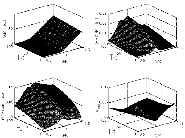
Figure 7: Option price and equivalent implied volatility in the ”risk-neutral” approach to the stochastic volatility model

In Fig.7 we plot the option value surface for $V\left(S_{t},\sigma_{t},t\right)$ in the range $T-t\in[5,100]$ and $S/K\in[0.5,1.5]$ as well as the difference $\left(V\left(S_{t},\sigma_{t},t\right)-C\left(S_{t},\sigma_{t},t\right)\right)/K$ for $k=1$ and $k=2$. The other parameters are fixed at $\sigma=0.01,r=0.001,\delta=1,H=0.8$.

To compare the predictions of our formula with the classical Black-Scholes (BS) result, we have computed the implied volatility required in the BS model to reproduce our results. This is plotted in the lower right panel of Fig.7 which shows the implied volatility surface corresponding to $V\left(S_{t},\sigma_{t},t\right)$ for $k=1$. One sees that, when compared to BS, it predicts a smile effect with the smile increasing as maturity approaches.

5 Conclusions

(a) In this paper, rather than starting by postulating some model for the market process and then exploring its better or worse vindication by the data, the approach has been to be inspired, at each step of its construction, both by mathematical simplicity and consistency with the data. It is mathematically more complex and requires (for example for a derivation of option pricing without assuming risk-neutrality) more sophisticated tools of Malliavin calculus than most stochastic volatility models. Nevertheless, from its very construction and consistency with the data, it appears as a kind of minimal model.

(b) The asymptotic behavior of price returns, in special its asymptotic behavior has been much discussed (see for example [20] and references therein). In particular it has been proposed that the large return tail decays as a power law, although a stretched exponential might provide a better fit[21].

The semilogarithmic plots suggest in fact that a better overall fit might be obtained by a stretched exponential or indeed by Eqs. (27) and (28).

(c) From the data and model comparison plotted in the figures it looks that the stochastic volatility model (as well as a scaling hypothesis) cannot fit the very large deviations. There is a good fit for the bulk of the data but there are also a few events very far from the fit. It suggests that a model with two probability spaces is still not enough to capture the whole process. Maybe one should write $S_{t}\left(\omega,\omega^{{}^{\prime}},\omega^{{}^{\prime\prime}}\right)$ with the last entry, $\omega^{{}^{\prime\prime}}$, representing exogenous market shocks.

References

• [1] Z. Ding, C. W. J. Granger and R. Engle; A long memory property of stock returns and a new model, Journal of Empirical Finance 1 (1993) 83-106.
• [2] A. C. Harvey; Long memory in stochastic volatility, Research report 10, London School of Economics, 1993.
• [3] F. J. Breidt, N. Crato and P. Lima; The detection and estimation of long memory in stochastic volatility models, J. of Econometrics 83 (1998) 325-348.
• [4] R. F. Engle; Autoregressive conditional heteroscedasticity with estimates of the variance of United Kingdom inflation, Econometrica 50 (1982) 987-1007.
• [5] S. J. Taylor; Modeling stochastic volatility: A review and comparative study, Mathematical Finance 4 (1994) 183-204.
• [6] R. S. Engle and A. J. Patton; What good is a volatility model ?, Quantitative Finance 1 (2001) 237-245.
• [7] D. Nualart; The Malliavin Calculus and Related Topics, Springer-Verlag, Berlin 1995.
• [8] R. Vilela Mendes, R. Lima and T. Araújo; A process-reconstruction analysis of market fluctuations, Int. J. of Theoretical and Applied Finance 5 (2002) 797-821.
• [9] M. S. Taqqu, V. Teverovsky and W. Willinger; Estimators for long-range dependence: an empirical study, Fractals 3 (1995) 785-788.
• [10] P. Embrechts and M. Maejima; Selfsimilar processes, Princeton Univ. Press, Princeton NJ 2002.
• [11] B. B. Mandelbrot and J. W. Van Ness; Fractional Brownian motions, fractional noises and applications, SIAM Rev. 10 (1968) 422-437.
• [12] F. Comte and E. Renault; Long memory in continuous-time stochastic volatility models, Mathematical Finance 8 (1998) 291-323.
• [13] A. C. Silva, R. E. Prange and V. M. Yakovenko; Exponential distribution of financial returns at mesoscopic time lags: A new stylized fact, Physica A344 (2004) 227-235.
• [14] A. A. Dragulescu and V. M. Yakovenko; Probability distribution of returns in the Heston model with stochastic volatility, Quantitative Finance 2 (2002) 443-453.
• [15] S. L. Heston; A closed form solution for options with stochastic volatility with applications to bond and currency options, The Review of Financial Studies 6 (1993) 327-343.
• [16] J. C. Cox and S. A. Ross; The valuation of options for alternative stochastic processes, J. of Financial Economics 3(1976) 145-166.
• [17] J. C. Hull and A. White; The pricing of options on assets with stochastic volatility, J. of Finance 42 (1987) 281-300.
• [18] F. Black and M. Scholes; The pricing of options and corporate liabilities, J. of Political Economy 81 (1973) 637-654.
• [19] R. C. Merton; Theory of rational option pricing, Bell J. Econ. Manag. Sci. 4 (1973) 141-183.
• [20] J. Töyli, M. Sysi-Aho and K. Kaski; Models of asset returns: changes of pattern from high to low event frequency, Quantitative Finance 4 (2004) 373-382.
• [21] Y. Malevergne, V. Pisarenko and D. Sornette; Empirical distributions of stock returns: between the stretched exponential and the power law, Quantitative Finance 5 (2005) 379-401.