\college

Jesus College \degreeDoctor of Philosophy \degreedateMichaelmas 2005

The Brownian Frame Process as a Rough Path

Ben Hoff
Abstract

The Brownian frame process $\mathcal{T}^{B}$ is defined as

$$\mathcal{T}_{t}^{B}:=\left(B_{t-1+u}\right)_{0\leq u\leq 1},\text{ \ \ }t\in\left[0,1\right],$$

where $B$ is a real-valued Brownian motion with parameter set $\left[-1,1\right]$. This thesis investigates properties of the path-valued Brownian frame process relevant to establishing an integration theory based on the theory of rough paths ([Lyons, 1998]). The interest in studying this object comes from its connection with Gaussian Volterra processes (e.g. [Decreusefond, 2005]) and stochastic delay differential equations (e.g. [Mohammed, 1984]). Chapter 2 establishes the existence of $\mathcal{T}^{B}$. We then examine the convergence of dyadic polygonal approximations to $\mathcal{T}^{B}$ if the path-space $V$ where $\mathcal{T}^{B}$ takes its values is equipped with first the $p$-variation norm ($p>2$) and second the $\sup$-norm. In the case of the $p$-variation norm, the Brownian frame process is shown to have finite $\acute{p}$-variation for $\acute{p}>\frac{2p}{p-2}$. In the case of the $\sup$-norm, it is shown to have finite $\acute{p}$-variation for $\acute{p}>2$. Chapter 3 provides a tail estimate for the probability that two evaluations of the Brownian frame process are far apart in the $p$-variation norm. Chapter 4 shows that $\mathcal{T}^{B}$ does not have a Lรฉvy area if $V\otimes V$ is equipped with the injective tensor product norm (where $V=C\left(\left[0,1\right]\right)$).


{dedication}

To my parents.

Acknowledgements.
My thanks go to my supervisor, Terry Lyons, without whom this thesis would never have happened. I am grateful to Ben Hambly and James Norris for their careful reading and valuable comments. As a recipient of a doctoral training grant Iย am endebted to EPSRC. I gratefully acknowledge the contribution of a Jesus College Old Members Graduate Scholarship. Most importantly, I want to thank my parents for their generosity in all respects.
{romanpages}

Chapter 1
Introduction

1.1 Motivation

Let $x_{.}:\left[0,t\right]\rightarrow V$, where $V~{}$is some linear space and

$$T:\left[0,t\right]\rightarrow\left[0,t\right]$$

be such that $T\left(h\right)\leq h$. By the historic frame path $\mathcal{T}^{x}$ of $x$, we mean the path-valued path

$$\mathcal{T}_{h}^{x}:=\left(x_{h-T\left(h\right)+u}\right)_{0\leq u\leq T\left(h\right)},\text{ \ \ }h\in\left[0,t\right].$$ (1.1)

$\mathcal{T}^{x}$ takes its values in the space of paths from $\left[0,T\left(h\right)\right]$ to $V$, i.e. $\mathcal{T}_{h}^{x}\in V^{\left[0,T\left(h\right)\right]}$ (where $V^{\left[a,b\right]}$ denotes the space of all paths from $\left[a,b\right]$ to $V$). The map

$$T:\left[0,t\right]\rightarrow\left[0,t\right]$$

determines the frame length of $\mathcal{T}^{x}$ at time $h$ so that the evaluation of $\mathcal{T}^{x}$ at time $h$ is a $V$-valued path of length $T\left(h\right)$.

Example 1

If $T\equiv 0$, then $\mathcal{T}^{x}\equiv x$.

We give two examples to illustrate the relevance of the historic frame path:

Example 2

From a control theory point of view, a differential equation is interpreted as follows: The system we want to control has state $y_{t}$ at time $t$ (where $y_{t}$ lives on some manifold $W$). The initial state is given by $y_{0}$. The driving signal $x_{t}$ that determines the state of the system at time $t$ lives on some Banach space $V$. It filters through a map

$$f\left(.\right):V\rightarrow\left(W\rightarrow TW\right)$$

to produce an effect in the state space $W$ (here $TW$ denotes the tangent space of $W$). We call $f$ the vector field map and write

$$dy_{u}=f\left(y_{u}\right)dx_{u},\text{ \ \ }y_{0}=a.$$ (1.2)

Subject to $f$ and $x$ satisfying certain conditions, [Lyons, 1998] gives meaning to (1.2) (the exact result is quoted in Theorem 1.2.15 below). In the classical theory of dynamical systems with memory (delay differential equations), the system response at time $r$ may depend on the entire solution trajectory up to time $r$, that is the vector field map $f$ is a function of the path segment $\left(y_{u}:0\leq u\leq r\right)$, so that

$$f\left(\left(y_{u}\right)_{0\leq u\leq r}\right):V\rightarrow TW.$$

The โ€œdelayโ€ย here occurs as an argument of the vector field map. One could imagine a dynamical system with a different type of memory where the delay occurs in the driving signal $x$: ย Since each state $y_{r}$ is determined by the initial state $y_{0}$ and the signal path segment $\left(x_{u}:0\leq u\leq r\right)$, an approach where $y$ is driven by the entire historic trajectory $\left(x_{u}:0\leq u\leq.\right)$ could prove to be interesting. In other words, we might like to give meaning to (1.2) in the sense of [Lyons, 1998] if the driving signal $x$ evaluated at time $r$ equals $\left(z_{u}\right)_{0\leq u\leq r}$ and $z$ is some $V$-valued path. In this case, $x=\mathcal{T}^{z}$ is the frame process defined in (1.1) associated to $z$ with variable frame length $T\left(h\right)=h$.

Example 3

We consider a Volterra Gaussian Process, say Fractional Brownian Motion (fBM) with Hurst parameter $H$. $B$ is a real-valued Brownian Motion. The evaluation of fBM at time $t$ is obtained by applying the Wiener integral to an appropriate deterministic $L^{2}$- kernel $K_{H}\left(t,.\right)$111The kernel $K_{H}$ is given by KHโ€‹(t,s)=CHโ€‹[22โ€‹Hโˆ’1โ€‹(tโ€‹(tโˆ’s)s)Hโˆ’12โˆ’โˆซst(uโ€‹(uโˆ’s)u)Hโˆ’12โ€‹dโ€‹uu]โ€‹๐Ÿ]0,t[โ€‹(s)subscript๐พ๐ป๐‘ก๐‘ subscript๐ถ๐ปdelimited-[]22๐ป1superscript๐‘ก๐‘ก๐‘ ๐‘ ๐ป12superscriptsubscript๐‘ ๐‘กsuperscript๐‘ข๐‘ข๐‘ ๐‘ข๐ป12๐‘‘๐‘ข๐‘ขsubscript10๐‘ก๐‘ K_{H}\left(t,s\right)=C_{H}\left[\frac{2}{2H-1}\left(\frac{t\left(t-s\right)}{s}\right)^{H-\frac{1}{2}}-\int_{s}^{t}\left(\frac{u\left(u-s\right)}{u}\right)^{H-\frac{1}{2}}\frac{du}{u}\right]\mathbf{1}_{\left]0,t\right[}\left(s\right) where $C_{H}=\frac{\Gamma\left(2-2H\right)\cos\left(\pi H\right)}{\Gamma\left(H-\frac{1}{2}\right)\pi H\left(1-2H\right)}.$,

fโ€‹Bโ€‹MHโ€‹(r):=โˆซ0rKHโ€‹(t,s)โ€‹๐‘‘Bs.assign๐‘“๐ตsubscript๐‘€๐ป๐‘Ÿsuperscriptsubscript0๐‘Ÿsubscript๐พ๐ป๐‘ก๐‘ differential-dsubscript๐ต๐‘ fBM_{H}\left(r\right):=\int_{0}^{r}K_{H}\left(t,s\right)dB_{s}.

This is a functional of the path-segment $\mathcal{T}^{B}\left(r\right)=\left(B_{u}:0\leq u\leq r\right)$ โ€“ i.e. a functional of the Brownian Frame Process of frame length $T\left(r\right)=r$.


This thesis investigates some of the rough path properties (c.f. [Lyons, 1998]) of the ย historic frame path on the Wiener space $\left(C_{0}\left(\left[-1,1\right]\right),\sigma_{\left\|.\right\|_{\infty}},\mathbb{P}\right)$222$C_{0}\left(\left[-1,1\right]\right)$ denotes the space of continuous functions on $\left[-1,1\right]$ that are 00 at $-1$. $\sigma_{\left\|.\right\|_{\infty}}$ denotes the completion of the $\sigma$-algebra generated by the $\sup$-norm and $\mathbb{P}$ is the Wiener measure., defined for $f\in C_{0}\left(\left[-1,1\right]\right)$ at $h\in\left[0,1\right]$ as

$$\mathcal{T}_{h}^{f}:=\left(f_{h-1+u}\right)_{0\leq u\leq 1}.$$ (1.3)

Here, we have a constant frame length $T\equiv 1$. When viewed as a (Borel) random variable on Wiener space, $\mathcal{T}_{h}^{B}$ will be called the Brownian frame random variable at $h$ (associated to the Brownian Motion $B$ supported on $\left(C_{0}\left(\left[-1,1\right]\right),\sigma_{\left\|.\right\|_{\infty}},\mathbb{P}\right)$).

1.2 Rough Path Theory

The theory of Rough Paths as developed in [Lyons, 1998] shows how to construct solutions to differential equations driven by paths that are not of bounded variation but have controlled roughness. The $p$-variation (Definitionย 7 below) is taken as a measure of a Banach space valued pathโ€™s roughness. The analysis is independent of the dimension of the Banach space and so appears particularly well adapted to the case where the Banach space in question is a path-space. We give a brief overview:

Let $V$ be a Banach space with norm $\left|.\right|_{V}$. We denote by $T^{n}\left(V\right)$ the truncated tensor algebra of $V$, that is

$$T^{n}\left(V\right):=\mathbb{R\oplus}V\oplus V^{\otimes 2}\oplus...\oplus V^{\otimes n},$$

where $V^{\otimes i}:=V\otimes V\otimes...\otimes V$ ($i$ copies).

Definition 4 (multiplicative functional)

A continuous functional

{๐ฑ:{(s,t):0โ‰คsโ‰คtโ‰คT}โ†’Tnโ€‹(V)๐ฑs,t=(xs,t0,xs,t1,xs,t2,โ€ฆ,xs,tn)cases:๐ฑโ†’conditional-set๐‘ ๐‘ก0๐‘ ๐‘ก๐‘‡superscript๐‘‡๐‘›๐‘‰subscript๐ฑ๐‘ ๐‘กsuperscriptsubscript๐‘ฅ๐‘ ๐‘ก0superscriptsubscript๐‘ฅ๐‘ ๐‘ก1superscriptsubscript๐‘ฅ๐‘ ๐‘ก2โ€ฆsuperscriptsubscript๐‘ฅ๐‘ ๐‘ก๐‘›\left\{\begin{array}[]{c}\mathbf{x}:\left\{\left(s,t\right):0\leq s\leq t\leq T\right\}\rightarrow T^{n}\left(V\right)\\ \mathbf{x}_{s,t}=\left(x_{s,t}^{0},x_{s,t}^{1},x_{s,t}^{2},...,x_{s,t}^{n}\right)\end{array}\right.

is called multiplicative if it satisfies Chenโ€™s identity

๐ฑs,tโŠ—๐ฑt,u=๐ฑs,uโ€‹ย forย โ€‹0โ‰คsโ‰คtโ‰คuโ‰คTโ€‹ย tensor-productsubscript๐ฑ๐‘ ๐‘กsubscript๐ฑ๐‘ก๐‘ขsubscript๐ฑ๐‘ ๐‘ขย forย 0๐‘ ๐‘ก๐‘ข๐‘‡ย \mathbf{x}_{s,t}\otimes\mathbf{x}_{t,u}=\mathbf{x}_{s,u}\text{ \ for }0\leq s\leq t\leq u\leq T\text{ }

and

xs,t0โ‰ก0โ€‹ย onย โ€‹{(s,t):0โ‰คsโ‰คtโ‰คT}.superscriptsubscript๐‘ฅ๐‘ ๐‘ก00ย onย conditional-set๐‘ ๐‘ก0๐‘ ๐‘ก๐‘‡x_{s,t}^{0}\equiv 0\text{ on }\left\{\left(s,t\right):0\leq s\leq t\leq T\right\}.
Example 5

Every continuous $V$-valued path $x$ determines a multiplicative functional (1,xtโˆ’xs)1subscript๐‘ฅ๐‘กsubscript๐‘ฅ๐‘ \left(1,x_{t}-x_{s}\right) in $T^{1}\left(V\right)$. The converse is not true: With every multiplicative functional $y\in T^{1}\left(V\right)$ we may associate a collection of $V$-valued paths $\left\{y_{0,t}^{1}+c:c\in V\right\}$.

A wide class of multiplicative functionals is given by

Theorem 6 (Chenโ€™s theorem)

Suppose $x$ is a bounded variation path in $V$. Then $x$ has a canonical multiplicative lift ๐ฑs,t=(xs,t0,xs,t1,โ€ฆ,xs,tn)subscript๐ฑ๐‘ ๐‘กsuperscriptsubscript๐‘ฅ๐‘ ๐‘ก0superscriptsubscript๐‘ฅ๐‘ ๐‘ก1โ€ฆsuperscriptsubscript๐‘ฅ๐‘ ๐‘ก๐‘›\mathbf{x}_{s,t}=\left(x_{s,t}^{0},x_{s,t}^{1},...,x_{s,t}^{n}\right) to $T^{n}\left(V\right)$ given by its sequence of iterated integrals:

xs,t0superscriptsubscript๐‘ฅ๐‘ ๐‘ก0\displaystyle x_{s,t}^{0} $\displaystyle\equiv$ 1,ย โ€‹xs,t1โ‰กxtโˆ’xs,formulae-sequence1ย superscriptsubscript๐‘ฅ๐‘ ๐‘ก1subscript๐‘ฅ๐‘กsubscript๐‘ฅ๐‘ \displaystyle 1,\text{ \ }x_{s,t}^{1}\equiv x_{t}-x_{s},\text{ \ }
ย โ€‹xs,tkย superscriptsubscript๐‘ฅ๐‘ ๐‘ก๐‘˜\displaystyle\text{\ }x_{s,t}^{k} $\displaystyle=$ โˆซโ€ฆโ€‹โˆซsโ‰คu1โ‰คu2โ‰คโ€ฆโ‰คukโ‰คt๐‘‘xu1โŠ—๐‘‘xu2โŠ—โ€ฆโŠ—๐‘‘xuk.โ€ฆsubscript๐‘ subscript๐‘ข1subscript๐‘ข2โ€ฆsubscript๐‘ข๐‘˜๐‘กtensor-productdifferential-dsubscript๐‘ฅsubscript๐‘ข1differential-dsubscript๐‘ฅsubscript๐‘ข2โ€ฆdifferential-dsubscript๐‘ฅsubscript๐‘ข๐‘˜\displaystyle\int...\int_{s\leq u_{1}\leq u_{2}\leq...\leq u_{k}\leq t}dx_{u_{1}}\otimes dx_{u_{2}}\otimes...\otimes dx_{u_{k}}.

We call $\mathbf{x}$ the Chen lift of $x$.

In general, if $\mathbf{y=}\left(y^{0},y^{1},y^{2},...,y^{m}\right)$ is a multiplicative functional with values in $T^{m}\left(V\right)$ and for some $\mathbf{z=}\left(z^{0},z^{1},z^{2},...,z^{n}\right)$ taking values in $T^{n}\left(V\right)$ with $m\geq n$, we have that

$$\mathbf{z}=\left(y^{0},y^{1},y^{2},...,y^{n}\right),$$

then we say that $\mathbf{z}$ is the projection of $\mathbf{y}$ onto $T^{n}\left(V\right)$. We also say that $\mathbf{y}$ is a multiplicative functional lying above $\mathbf{z}$ or that $\mathbf{y}$ is a lift of $\mathbf{z}$. It is important to note that in general for a given $\mathbf{z}$, neither existence nor uniqueness of $\mathbf{y}$ is obvious (Theorem 1.2.14ย below deals with the existence of a unique lift for a particular class of $\mathbf{z}$).

For each $n$, $V^{\otimes n}$ is assumed to be equipped with a compatible tensor norm $\left\|.\right\|_{V^{\otimes n}}$: If $v\in V^{\otimes i}$ and $w\in V^{\otimes j}$, then $\left\|.\right\|_{V^{\otimes n}}$ is said to be compatible if for any $\left(i,j\right)$ with $i+j\leq n$, we have

$$\left\|v\otimes w\right\|_{V^{\otimes\left(i+j\right)}}\leq\left\|v\right\|_{V^{\otimes i}}\left\|w\right\|_{V^{\otimes j}},$$ (1.4)

and

$$\left\|v\right\|_{V^{\otimes 1}}\equiv\left|v\right|_{V}.$$
Definition 7

Let $\mathcal{D}\left(\left[0,T\right]\right)$ denote the set of all finite dissections of $\left[0,1\right]$, that is

$$\mathcal{D}\left(\left[0,T\right]\right):=\left\{\left\{t_{0},t_{1,},...,t_{n}\right\}:t_{0}=0<t_{1}<t_{2}<...<t_{n}=T\text{ and }n\text{ is finite}\right\}.$$

For $p\geq n$, the $p$-variation functional of level $i$ of a function

๐ฑ:{(s,t):0โ‰คsโ‰คtโ‰คT}โ†’Tnโ€‹(V):๐ฑโ†’conditional-set๐‘ ๐‘ก0๐‘ ๐‘ก๐‘‡superscript๐‘‡๐‘›๐‘‰\mathbf{x}:\left\{\left(s,t\right):0\leq s\leq t\leq T\right\}\rightarrow T^{n}\left(V\right)

with

๐ฑs,t=(xs,t0,xs,t1,xs,t2,โ€ฆ,xs,tn)subscript๐ฑ๐‘ ๐‘กsuperscriptsubscript๐‘ฅ๐‘ ๐‘ก0superscriptsubscript๐‘ฅ๐‘ ๐‘ก1superscriptsubscript๐‘ฅ๐‘ ๐‘ก2โ€ฆsuperscriptsubscript๐‘ฅ๐‘ ๐‘ก๐‘›\mathbf{x}_{s,t}=\left(x_{s,t}^{0},x_{s,t}^{1},x_{s,t}^{2},...,x_{s,t}^{n}\right)

is defined as

$$\mathcal{V}_{p}\left(x^{i}\right):=\sup\left\{\sum_{D}\left\|x_{t_{j-1},t_{j}}^{i}\right\|_{V^{\otimes i}}^{\frac{p}{i}}:D\in\mathcal{D}\left(\left[0,T\right]\right)\right\}^{\frac{i}{p}}.$$

$\mathbf{x}$ is said to have finite $p$-variation if

$$\mathcal{V}_{p}\left(\mathbf{x}\right):=\max_{1\leq i\leq n}\mathcal{V}_{p}\left(x^{i}\right)$$

is finite.

Definition 8 (rough path)

A multiplicative functional of finite $p$-variation with values in $T^{\left\lfloor p\right\rfloor}\left(V\right)$ (where $\left\lfloor p\right\rfloor:=\max\left(n\in\mathbb{N}:n\leq p\right)$) is called a rough path of roughness $p$. The set of all $p$-rough paths is denoted as $\Omega_{p}\left(V\right).$ For any $\mathbf{x,y}\in$ $\Omega_{p}\left(V\right)$, the $p$-variation distance $d_{p}$ is defined as

$$d_{p}\left(\mathbf{x,y}\right)=\mathcal{V}_{p}\left(\mathbf{x-y}\right)\text{.}$$
Remark 9

$\left(\Omega_{p}\left(V\right),d_{p}\right)$ is a complete metric space as are all projections of $\Omega_{p}\left(V\right)$ onto $T^{n}\left(V\right)$ for $n\leq\left\lfloor p\right\rfloor$ (Lemma 3.3.3 in [Lyons and Qian, 2002]). However, $\Omega_{p}\left(V\right)$ is not a linear space โ€“ in general, the sum of two multiplicative functionals fails to be multiplicative.

Lemma 10

If $\acute{p}\geq p$, then $d_{\acute{p}}\leq d_{p}$.

Proof 1.2.11.

For $\left(a_{j}\right)_{1\leq j\leq n}\in\mathbb{R}^{n}$,

$\displaystyle\left[\sum_{j=1}^{n}\left|a_{j}\right|\right]^{\frac{\acute{p}}{p}}$ $\displaystyle=$ $\displaystyle\left[\sum_{j=1}^{n}\left|a_{j}\right|\right]\left[\sum_{j=1}^{n}\left|a_{j}\right|\right]^{\frac{\acute{p}}{p}-1}$
$\displaystyle=$ $\displaystyle\sum_{j=1}^{n}\left|a_{j}\right|\left[\sum_{i=1}^{n}\left|a_{i}\right|\right]^{\frac{\acute{p}}{p}-1}\geq\sum_{j=1}^{n}\left|a_{j}\right|^{\frac{\acute{p}}{p}}.$

We now fix $\mathbf{x}\in\Omega_{p}\left(V\right)$ and a dissection $D$ in $\mathcal{D}\left(\left[0,T\right]\right)$ (Definition 7 above). If we take $\left|a_{j}\right|=\left|x_{t_{j},t_{j+1}}^{i}\right|^{\frac{p}{i}}$ for $1\leq i\leq p$ and then take the $\sup$ over $\mathcal{D}\left(\left[0,T\right]\right)$, the result follows (we set xs,tnโ‰ก0superscriptsubscript๐‘ฅ๐‘ ๐‘ก๐‘›0x_{s,t}^{n}\equiv 0 for $p<n\leq\acute{p}$).

Definition 1.2.12 (smooth rough path).

Suppose $x$ is a bounded variation path in $V$. We will denote by $\mathbf{x}$ the Chen lift of $x$ to $T^{n}\left(V\right)$ and call $\mathbf{x}$ a smooth rough path. The collection of smooth rough paths is contained in $\cap_{p\geq 1}\Omega_{p}\left(V\right)$.

Definition 1.2.13 (geometric rough path).

The closure of the smooth rough paths under $d_{p}$ is called the space of geometric rough pathsย of roughness $p$ and denoted $\Omega G\left(V\right)_{p}$.

The โ€œFirst Theoremโ€ย from [Lyons, 1998] gives sufficient conditions for the existence of a unique lift:

Theorem 1.2.14 (Theorem 2.2.1 in [Lyons, 1998]).

Let ๐—s,t(n)superscriptsubscript๐—๐‘ ๐‘ก๐‘›\mathbf{X}_{s,t}^{\left(n\right)} be a continuous multiplicative functional in $T^{\left(n\right)}\left(V\right)$ of finite $p$-variation where $n=\left\lfloor p\right\rfloor$. There exists a multiplicative extension ๐—s,t(m)superscriptsubscript๐—๐‘ ๐‘ก๐‘š\mathbf{X}_{s,t}^{\left(m\right)} to $T^{\left(m\right)}\left(V\right)$, $m>n$ which is of finite $p$-variation. The extension is unique in this class.

The Universal Limit Theorem below establishes the connection between multiplicative functionals and solutions to differential equations:

Theorem 1.2.15 ( Theorem 4.1.1 in [Lyons, 1998]).

Let $f$ be a linear map from $V$ to the space of Lipschitz-$\gamma$ vector fields on $W$, that is $f\in L\left(V,Lip\left(\gamma,W,W\right)\right)$ 333$Lip\left(n+\varepsilon,W,W\right)$ denotes the space of $n$-times differentiable functions from $W$ to $W$ whose $n^{\text{th}}$ derivative is $\varepsilon$-Lipschitzwhere $1\leq p<\gamma$. Then consider the Itรด map $I:X\rightarrow\left(X,Y\right)$ defined for bounded variation paths by

$$dY_{t}=f\left(Y_{t}\right)dX_{t},\text{ \ \ \ }Y_{0}=a.$$ (1.5)

Define the one form $h$ by

$$h\left(x,y\right)\left(dX,dY\right)=h\left(y\right)\left(dX,dY\right)=\left(dX,f\left(y\right)dX\right).$$

For any geometric multiplicative functional $\mathbf{X}\in\Omega G\left(V\right)_{p}$ there is exactly one geometric multiplicative functional extension $\mathbf{Z=}\left(\mathbf{X,Y}\right)\in\Omega G\left(V\oplus W\right)_{p}$ such that if $Y_{t}=$ $\mathbf{Y}_{0,t}^{1}+a,$ then $\mathbf{Z}$ satisfies the rough444By a rough differential equation we mean a differential equation on the truncated tensor algebra $T^{n}\left(V\right)$. To emphasise the difference between a differential equation and a rough differential equation we write โ€œฮดโ€‹๐™๐›ฟ๐™\delta\mathbf{Z}โ€ย instead of โ€œdโ€‹๐™๐‘‘๐™d\mathbf{Z}โ€(c.f Definition 4.1.1 in [Lyons, 1998])ย  differential equation

$$\delta\mathbf{Z=}h\left(\mathbf{Y}_{t}\right)\delta\mathbf{Z}.$$

Such a solution exists on a small interval $\left[0,T\right]$ whose length can be controlled entirely in terms of the control of the roughness of $X$ and of $f$ . The Itรด map is uniformly continuous and the map $\mathbf{X\rightarrow Z}$ is the unique continuous extension of the Itรด map from $\Omega G\left(V\right)^{p}$ to $\Omega G\left(V\oplus W\right)^{p}$.

1.3 Results

In Chapter $2$ we establish the existence of a continuous Brownian frame process $\mathcal{T}^{B}$ into $\left(C\left(\left[0,1\right]\right),\left\|.\right\|_{\infty}\right)$. $\mathcal{T}^{B}$ algebraically agrees with the object defined in (1.3), i.e. for any $f\in C_{0}\left(\left[-1,1\right]\right)$, $\mathcal{T}^{B}\left(f\right):=\mathcal{T}^{f}$. We call $\mathcal{T}^{B}$ the Brownian $\sup$-frame process.ย Forย pยด>2,ยด๐‘2\acute{p}>2, $\mathcal{T}_{.}^{B}$ is shown to have finite $\acute{p}$-variation. Furthermore, the dyadic polygonal approximations of $\mathcal{T}^{B}$ converge to $\mathcal{T}^{B}$ in $\acute{p}$-variation.

If $p\geq 1$, $\left(C\left(\left[0,1\right]\right)_{p},\left\|.\right\|_{p}\right)$ denotes the Banach space of continuous functions of finite $p$-variation equipped with the $p$-variation norm

$$\left\|.\right\|_{p}:=\left\|.\right\|_{\infty}+\mathcal{V}_{p}\left(.\right).$$

For $p>2$, we establish the existence of a continuous Brownian frame process $\mathcal{S}_{.}^{B,p}$ into $\left(C\left(\left[0,1\right]\right)_{p},\left\|.\right\|_{p}\right)$ that algebraically agrees with the object defined in (1.3) off a nullset. That is, $\mathcal{S}^{B,p}\left(f\right)$ is equal to $\mathcal{T}^{f}$ for $\mathbb{P}$-a.e. $f\in C_{0}\left(\left[-1,1\right]\right).$ ย ๐’ฎB,psuperscript๐’ฎ๐ต๐‘\mathcal{S}^{B,p} is called the $p$-variation frame process. For $\acute{p}>\frac{2p}{p-2}$, we show that the dyadic polygonal approximations of $\mathcal{S}^{B,p}$ converge to $\mathcal{S}_{.}^{B,p}$ in $\acute{p}$-variation.

In Chapter $3$, we examine further properties of $\mathcal{S}^{B,p}$ ($p>2$): We find constants, $d_{1}\left(\alpha,p\right)$ ย ($\alpha$ is a constant strictly greater than $1-\frac{1}{p}$) and $d_{2}\left(p\right)$, so that the random variable

$$\frac{\left\|\mathcal{S}_{h_{2}}^{B,p}-\mathcal{S}_{h_{1}}^{B,p}\right\|_{p}}{d_{2}\left(p\right)\left(h_{2}-h_{1}\right)^{\frac{1}{2}-\frac{1}{p}}}-d_{1}\left(\alpha,p\right)$$

has Gaussian tails. More precisely, we find constants $d_{1}\left(\alpha,p\right)$ and $d_{2}\left(p\right)$ such that

$$\mathbb{P}\left(\frac{\left\|\mathcal{S}_{h_{2}}^{B,p}-\mathcal{S}_{h_{1}}^{B,p}\right\|}{d_{2}\left(p\right)\left(h_{2}-h_{1}\right)^{\frac{1}{2}-\frac{1}{p}}}-d_{1}\left(\alpha,p\right)>r\right)\leq\frac{1}{\sqrt{2\pi}r}\exp\left(-\frac{r^{2}}{2}\right).$$

In Chapter $4$ we are concerned with the $\sup$-frame process $\mathcal{T}^{B}$. The Universal Limit Theorem (Theorem 1.2.15 above) tells us how to solve differential equations driven by rough paths โ€“ย provided the driving signal is the level $1$ projection of some geometric $\acute{p}$-rough path. Since

$$\mathcal{T}^{B}:\left[0,1\right]\rightarrow C\left(\left[0,1\right],\left\|.\right\|_{\infty}\right)$$

has finite $\acute{p}$-variation for $\acute{p}>2$, by Theorem 1.2.14, any lift of $\mathcal{T}^{B}$ to $T^{2}\left(V\right)$ that preserves finite $\acute{p}$-variation establishes an integration theory for $\mathcal{T}^{B}$ (here, $V=\left(C\left(\left[0,1\right]\right),\left\|.\right\|_{\infty}\right)$). From Chapter 2 we know that the (smooth) dyadic polygonal approximations $\mathcal{T}^{B}\left(m\right)$ of $\mathcal{T}^{B}$ converge to $\mathcal{T}^{B}$ in $\acute{p}$-variation norm. So it is natural to ask whether the lifts of $\mathcal{T}^{B}\left(m\right)$ converge in $T^{2}\left(V\right)$, thereby providing a natural lift of $\mathcal{T}^{B}$ to $T^{2}\left(V\right)$. We show that while the canonical lifts of the dyadic polygonal approximations to $\mathcal{T}^{B}$ converge, the convergence is to an object that lives outside the injective tensor product $V\otimes_{\vee}V$: After proving that $V\otimes_{\vee}V$ is isomorphic to $C\left(\left[0,1\right]\times\left[0,1\right]\right)$, we show that the Lรฉvy Area $\mathcal{A}_{0,1}\left(\mathcal{T}^{B}\right)$ of $\mathcal{T}^{B}$ โ€“ which is the limit of the antisymmetric component of $\int\int_{0\leq u\leq v\leq 1}d\mathcal{T}^{B}\left(m\right)_{u}\otimes d\mathcal{T}^{B}\left(m\right)_{v}$ as $m\rightarrow\infty$ โ€“ is continuous off the diagonal of the unit square. However, it is shown to have a jump-discontinuity on the diagonal and so does not exist in $V\otimes_{\vee}V$.

We believe that a further examination of the โ€œobstructionโ€ย โ€“ which is intimately linked to the quadratic variation of Brownian motion โ€“ will prove interesting and important.

Chapter 2
The Brownian frame process

2.1 Notation

We work on the classical Wiener Space $\left(C_{0}\left(\left[-1,1\right],\mathbb{R}\right),\sigma_{\left\|.\right\|_{\infty}},\mathbb{P}\right)$. Here,

$$C_{0}\left(\left[-1,1\right]\right):=\left\{f\in C\left(\left[-1,1\right]\right):f\left(-1\right)=0\right\}$$

and $\sigma_{\left\|.\right\|_{\infty}}$ denotes the completion of the Borel $\sigma$-algebra generated by the sup-norm

$$\left\|f\right\|_{\infty}:=\sup\left\{\left|f\left(t\right)\right|:t\in\left[-1,1\right]\right\},$$

with respect to the Wiener measure $\mathbb{P}$.

$B$ denotes the coordinate process

$$B_{t}:C_{0}\left(\left[-1,1\right]\right)\rightarrow\mathbb{R}:B_{t}\left(f\right):=f\left(t\right)\text{ \ \ },t\in\left[-1,1\right]$$

(on $C_{0}\left(\left[-1,1\right]\right)$) which (under Wiener measure $\mathbb{P}$) is a Brownian Motion.

$C\left(\left[a,b\right]\right)_{p}$ denotes the space of continuous real-valued paths on $\left[a,b\right]$ of finite $p$-variation, i.e.

$$C\left(\left[a,b\right]\right)_{p}=\left\{f\in C\left(\left[a,b\right]\right):\mathcal{V}_{p}\left(f^{1}\right)<\infty\right\},$$

where f1โ€‹(s,t):=fโ€‹(t)โˆ’fโ€‹(s)assignsuperscript๐‘“1๐‘ ๐‘ก๐‘“๐‘ก๐‘“๐‘ f^{1}\left(s,t\right):=f\left(t\right)-f\left(s\right) (c.f. Theorem 6 in Chapter 1) and the $p$-variation functional of level $1$ โ€“ ๐’ฑp(.)\mathcal{V}_{p}\left(.\right) โ€“ is defined in Definition 7 in Chapter 1.

Similarly, $C_{0}\left(\left[a,b\right]\right)_{p}$ denotes the space of continuous functions of finite $p$-variation that are 00 at $a$, i.e.

$$C_{0}\left(\left[a,b\right]\right)_{p}=\left\{f\in C_{0}\left(\left[a,b\right]\right):\mathcal{V}_{p}\left(f^{1}\right)<\infty\right\}.$$

When $f\in C\left(\left[a,b\right]\right)_{p}$, we say that $f$ has finite $p$-variation. We write $\mathcal{V}_{p}\left(f\right)$ in place of $\mathcal{V}_{p}\left(f^{1}\right)$ and in this way view $\mathcal{V}_{p}\left(.\right)$ as a functional on $C\left(\left[a,b\right]\right)_{p}$ .

From Chapter 1 we recall that $\mathcal{V}_{p}\left(.\right)+\left\|.\right\|_{\infty}$ is the $p$-variation norm on $C\left(\left[0,1\right]\right)_{p}$ for which we write

$$\left\|.\right\|_{p}:=\mathcal{V}_{p}\left(.\right)+\left\|.\right\|_{\infty}.$$

For the Banach space $C\left(\left[0,1\right]\right)_{p}$ equipped with $\left\|.\right\|_{p}$ we write $\left(C\left(\left[0,1\right]\right)_{p},\left\|.\right\|_{p}\right)$. When the norm is not explicitly mentioned, $C\left(\left[0,1\right]\right)_{p}$ is viewed as a subspace of $\left(C\left(\left[0,1\right]\right),\left\|.\right\|_{\infty}\right)$.

For $\alpha>1-\frac{1}{p}$ and $p>1$, we define the function $c\left(.,.\right)$ as

$$c\left(\alpha,p\right):=\left(\sum_{n=1}^{\infty}n^{-\alpha\frac{p}{p-1}}\right)^{\frac{p-1}{p}}.$$ (2.1)

The evaluation at $h\in\left[0,1\right]$ of the (deterministic) frame operator $\mathcal{T}_{.}\mathcal{\ }$on the set of functions from $\left[-1,1\right]$ to $\mathbb{R}$ โ€“ denoted as $\mathbb{R}^{\left[-1,1\right]}$ โ€“ is defined as

$$\left\{\begin{array}[]{c}\mathcal{T}_{h}^{.}:\mathbb{R}^{\left[-1,1\right]}\rightarrow\mathbb{R}^{\left[0,1\right]}\\ \mathcal{T}_{h}^{f}=\left(f\left(h-1+u\right)\right)_{u\in\left[0,1\right]}\end{array}\right..$$

We will be interested in $\mathcal{T}_{h}$ as a function on Wiener space and so will be considering the restriction of $\mathcal{T}_{h}$ to $C_{0}\left(\left[-1,1\right]\right)$.

If $M=\left\{x_{1},x_{2},...,x_{n}\right\}$, we write $\left\|M\right\|$ to denote the number of elements in $M$, i.e. $\left\|M\right\|=n$.

The $\Gamma$-function is defined as $\Gamma\left(t\right):=\int_{0}^{\infty}x^{t-1}e^{-x}dx$.

$D\left(\left[0,1\right]^{d}\right)$ is the $d$-dimensional unit cube of dyadic rationals, i.e.

$$D\left(\left[0,1\right]^{d}\right):=\left(\bigcup_{n\in\mathbb{N}}\left\{\frac{k}{2^{n}}:0\leq k\leq 2^{n}\right\}\right)^{d},$$ (2.2)

and for $u,t\in\left[0,1\right]^{d}$ , โ€œuโ‰ฅt๐‘ข๐‘กu\geq tโ€ย means that

$$u_{i}\geq t_{i}\text{ \ \ \ for \ }1\leq i\leq d\text{.}$$

Finally, for any $h\in\left[0,1\right]$, $n\left(h\right)$ denotes the unique integer such that $2^{-n\left(h\right)}\leq h<2^{-n\left(h\right)+1}$.

2.2 Main Results

In the following section, we show that for every fixed $h\in\left[0,1\right]$, $\left.\mathcal{T}_{h}\right|_{C_{0}\left(\left[-1,1\right]\right)}$ is a Borel random variable on Wiener space, mapping into $\left(C\left(\left[0,1\right]\right),\left\|.\right\|_{\infty}\right)$. In order to distinguish between the algebraic frame operator $\mathcal{T}_{h}$ (which we recall is into $\mathbb{R}^{\left[0,1\right]}$ without a topology) and the analytic object that is the Borel random variable into $\left(C\left(\left[0,1\right]\right),\left\|.\right\|_{\infty}\right)$, we write

$$\mathcal{T}_{h}^{B}:=\left.\mathcal{T}_{h}^{.}\right|_{C_{0}\left(\left[-1,1\right]\right)}.$$

We show that $\mathcal{T}^{B}$ has continuous sample paths. As mentioned in Chapter $1$, $\mathcal{T}^{B}$ is called the $\sup$-frame-process.

For $p>2,$ we show that for any fixed $h\in\left[0,1\right]$ the function

$$\mathcal{T}_{h}^{B,p}:=\left\{\begin{array}[]{ll}\mathcal{T}_{h}^{B}&\text{on }C_{0}\left(\left[-1,1\right]\right)_{p}\\ 0&\text{otherwise}\end{array}\right.$$ (2.3)

is a Borel random variable on Wiener space.

We produce Hรถlder-type moment bounds for $\left\|\mathcal{T}_{h_{2}}^{B}-\mathcal{T}_{h_{1}}^{B}\right\|_{\infty}$ and $\left\|\mathcal{T}_{h_{2}}^{B,p}-\mathcal{T}_{h_{1}}^{B,p}\right\|_{p}$. In the case of $\mathcal{T}^{B,p}$, we use Kolmogorovโ€™s lemma to show that there exists a modification with continuous sample paths. We denote this continuous modification as $\mathcal{S}^{B,p}$ and call it the $p$-variation frame process. We then show that if $\acute{p}>\frac{2p}{p-2}$, the dyadic polygonal approximations of $\mathcal{S}^{B,p}$ converge to $\mathcal{S}^{B,p}$ in $\acute{p}$-variation,ย โ„™โ„™\mathbb{P}-a.s. In the case of $\mathcal{T}^{B}$ we deduce that $\mathcal{T}^{B}$ has finite $\acute{p}$-variation for $\acute{p}>2$, $\mathbb{P}$-a.s, and that the polygonal dyadic approximations of $\mathcal{T}^{B}$ converge to $\mathcal{T}^{B}$ in $\acute{p}$-variation, $\mathbb{P}$-a.s.

2.3
Existence of the Brownian Frame random variable

2.3.1
The $\sup$-norm frame process $\mathcal{T}^{B}$

Lemma 2.3.16.

For any $h\in\left[0,1\right]$, $\mathcal{T}_{h}^{B}$ is continuous and hence Borel measurable.

Proof 2.3.17.

Fix $\varepsilon>0$. Suppose $f,g\in C_{0}\left(\left[-1,1\right]\right)$ and that $\left\|f-g\right\|_{\infty}<\delta=\varepsilon.$ Then

$$\sup_{u\in\left[0,1\right]}\left|f\left(h-1+u\right)-g\left(h-1+u\right)\right|\leq\left\|f-g\right\|_{\infty}<\varepsilon\text{.}$$
Lemma 2.3.18.

The $\sup$-norm frame process $\mathcal{T}^{B}$ has continuous sample paths.

Proof 2.3.19.

Fix $f\in C_{0}\left(\left[-1,1\right]\right)$ and $\varepsilon>0$. Since $\left[-1,1\right]$ is compact, $f$ is uniformly continuous, so that $\exists\delta_{\varepsilon}>0$ such that $\left|x-y\right|<\delta_{\varepsilon}\Longrightarrow\left|f\left(x\right)-f\left(y\right)\right|<\varepsilon$, i.e.

$$\sup_{x,y\in\left[-1,1\right]:\left|x-y\right|<\delta_{\varepsilon}}\left|f\left(y\right)-f\left(x\right)\right|\leq\varepsilon\text{,}$$

and so for $\left|h_{2}-h_{1}\right|<\delta_{\varepsilon}$,

$\displaystyle\sup_{u\in\left[0,1\right]}\left|\mathcal{T}_{h_{2}}^{f}\left(u\right)-\mathcal{T}_{h_{1}}^{f}\left(u\right)\right|$
$\displaystyle=$ $\displaystyle\sup_{u\in\left[0,1\right]}\left|f\left(h_{2}-1+u\right)-f\left(h_{1}-1+u\right)\right|$
$\displaystyle\leq$ $\displaystyle\sup_{x,y\in\left[-1,1\right]:\left|x-y\right|<\delta_{\varepsilon}}\left|f\left(y\right)-f\left(x\right)\right|\leq\varepsilon.$

2.3.2 The $p$-variation-norm frame process $\mathcal{S}^{B,p}$

We regard the $p$-variation functional $\mathcal{V}_{p}$ as a functional on $\left(C\left(\left[0,1\right]\right)_{p},\left\|.\right\|_{\infty}\right)$ and prove that it is lower semi-continuous as a map

$$\mathcal{V}_{p}:\left(C\left(\left[0,1\right]\right)_{p},\left\|.\right\|_{\infty}\right)\rightarrow\left(\mathbb{R}^{+},\left|.\right|\right).$$
Definition 2.3.20.

A real valued function $f$ defined on a topological space $\left(X,\tau_{X}\right)$ is lower semi-continuous if for any $\alpha\in\mathbb{R}$ the set $\left\{x\in X:f\left(x\right)\leq\alpha\right\}$ is closed.

So any lower-semicontinuous real-valued function is Borel-measurable.ย 

Lemma 2.3.21.

A real-valued function $f$ is lower semi-continuous iff ย xnโ†’xโ†’subscript๐‘ฅ๐‘›๐‘ฅx_{n}\rightarrow x, then $\lim\inf f\left(x_{n}\right)\geq f\left(x\right)$.

Proof 2.3.22.

$\Longrightarrow$: Fix any $\alpha\in\mathbb{R}$ and consider $M_{\alpha}=\left\{f\left(x\right)\leq\alpha\right\}$. Suppose $\left\{x_{n}:n\in\mathbb{N}\right\}\subset M_{\alpha}$ and $x_{n}\rightarrow x$. Since $f\left(x_{n}\right)\leq\alpha$ for all $n\in\mathbb{N}$, it follows that $\lim\inf f\left(x_{n}\right)\leq\alpha$. But by assumption $f\left(x\right)\leq\lim\inf f\left(x_{n}\right)\leq\alpha$, so that $x\in M_{\alpha}$. Thus, $M_{\alpha}$ is closed.

$\Longleftarrow$: Let $m:=\lim\inf f\left(x_{n}\right)$ and fix $\varepsilon>0$. An infinite subsequence of $\left(x_{n}\right)$ is contained in $A_{\varepsilon}:=\left\{x\in X:f\left(x\right)\leq m+\varepsilon\right\}$. Hence, $x\in A_{\varepsilon}$ for all $\varepsilon>0$. Hence, $f\left(x\right)\leq m$.

Proposition 2.3.23.

We recall the definition of the $p$-variation functional (c.f. Definition 7): Let $\mathcal{D}\left(\left[0,1\right]\right)$ denote the set of all finite dissections of $\left[0,1\right]$. If $p\geq 1$, the $p$-variation functional $\mathcal{V}_{p}$ on $C\left(\left[0,1\right]\right)_{p}$, defined as

$$\mathcal{V}_{p}:C\left(\left[0,1\right]\right)_{p}\rightarrow\mathbb{R}^{+}:\mathcal{V}_{p}\left(f\right):=\sup\left\{\sum_{D}\left|f\left(t_{i+1}\right)-f\left(t_{i}\right)\right|^{p}:D\in\mathcal{D}\left(\left[0,1\right]\right)\right\}^{\frac{1}{p}}$$

is lower-semicontinuous.

Proof 2.3.24.

Fix $f\in C\left(\left[0,1\right]\right)_{p}$. Suppose that $f_{n}\in C\left(\left[0,1\right]\right)$ and that $f_{n}\rightarrow f$. ย Since $\left[0,1\right]$ is compact and $f$ and $\left\{f_{n}\,:n\in\mathbb{N}\right\}$ are continuous, we may assume w.l.o.g. that the sequence $\left(f_{n}\right)$ is uniformly bounded by $K<\infty$, i.e. that $\sup_{n\in\mathbb{N}}\left\|f_{n}\right\|_{\infty}<K$.ย Since $f$ ย has finite $p$-variation, $\mathcal{V}_{p}^{p}\left(f\right)=c<\infty$, there exists a sequence of dissections $\left(D_{m}\right)_{m\in\mathbb{N}}$ with

$$D_{m}=\left\{t_{0}^{\left(m\right)}=0;t_{1}^{\left(m\right)};t_{2}^{\left(m\right)};...;t_{\left\|D_{m}\right\|}^{\left(m\right)}=1\right\}\in\mathcal{D}\left(\left[0,1\right]\right)$$

such that

$$\mathcal{V}_{p}^{p}\left(\sum_{D_{m}}f\left(t_{j}^{\left(m\right)}\right)\mathbf{1}_{\left[t_{j}^{\left(m\right)},t_{j+1}^{\left(m\right)}\right)}\right)\rightarrow c.$$

In other words: the sequence of step-functions defined as

$$\hat{f}_{m}=\sum_{j=0}^{\left\|D_{m}\right\|-1}f\left(t_{j}^{\left(m\right)}\right)\mathbf{1}_{\left[t_{j}^{\left(m\right)},t_{j+1}^{\left(m\right)}\right)},$$

converges to $f$ in $p$-variation. We start by fixing $\varepsilon>0$. W.l.o.g. we may assume that $\left\|D_{m}\right\|$ is non-decreasing (otherwise we eventually end up with the trivial dissection $\left\{0,1\right\}$) so that we may choose

$$\delta_{m}:=\frac{\varepsilon}{\left\|D_{m}\right\|2^{p}pK^{p-1}}.$$

By definition of $\hat{f}_{m}$, $\exists N_{\varepsilon}^{1}$ such that

$$\inf_{m>N_{\varepsilon}^{1}}\mathcal{V}_{p}^{p}\left(\hat{f}_{m}\right)>c-\varepsilon,$$

and since $f_{n}\rightarrow f$ in $C\left(\left[0,1\right]\right)$ and $\left[0,1\right]$ is compact, $\exists N_{\varepsilon,m}^{2}$ such that

$$\sup_{n>N_{\varepsilon,m}^{2}}\left\|f_{n}-f\right\|_{\infty}<\delta_{m}\text{.}$$

Fix $m>N_{\varepsilon}^{1}$ and $n>N_{\varepsilon,m}^{2}$ and consider any $t_{i}^{\left(m\right)},t_{i+1}^{\left(m\right)}\in D_{m}$. Then

$\displaystyle\left|f_{n}\left(t_{i+1}^{\left(m\right)}\right)-f_{n}\left(t_{i}^{\left(m\right)}\right)\right|$
$\displaystyle\geq$ $\displaystyle\left|f\left(t_{i+1}^{\left(m\right)}\right)-f\left(t_{i}^{\left(m\right)}\right)\right|-2\delta_{m}.$

By the mean value theorem, for any differentiable function $g$ on $\left[x-\lambda,x\right]$,

$$g\left(x\right)\leq g\left(x-\lambda\right)+\lambda\sup_{t\in\left[x-\lambda,x\right]}\left|g^{\prime}\left(t\right)\right|.$$ (2.5)

In particular, we choose $g\left(x\right)=x^{p}$ and $\lambda=2\delta_{m}$ and apply (2.5) to the right hand side of (2.3.24), noting that

$$\min_{t_{j}^{\left(m\right)},t_{j+1}^{\left(m\right)}\in D_{m}}\left|f\left(t_{j+1}^{\left(m\right)}\right)-f\left(t_{j}^{\left(m\right)}\right)\right|\leq\left|f\left(t_{i+1}^{\left(m\right)}\right)-f\left(t_{i}^{\left(m\right)}\right)\right|\leq 2K.$$

We then get

$$\left(\left|f\left(t_{i+1}^{\left(m\right)}\right)-f\left(t_{i}^{\left(m\right)}\right)\right|\right)^{p}\leq\left|f_{n}\left(t_{i+1}^{\left(m\right)}\right)-f_{n}\left(t_{i}^{\left(m\right)}\right)\right|^{p}+2^{p}\delta_{m}pK^{p-1}.$$

Hence,

$\displaystyle c-\varepsilon$ $\displaystyle\leq$ $\displaystyle\inf_{m>N_{\varepsilon}^{1}}\mathcal{V}_{p}^{p}\left(\hat{f}_{m}\right)$
$\displaystyle\leq$ $\displaystyle\inf_{m>N_{\varepsilon}^{1}}\inf_{n>N_{\varepsilon,m}^{2}}\left(\mathcal{V}_{p}^{p}\left(\sum_{D_{m}}f_{n}\left(t_{j}^{\left(m\right)}\right)\mathbf{1}_{\left[t_{j}^{\left(m\right)},t_{j+1}^{\left(m\right)}\right]}\right)\right.$
$\displaystyle\left.+2^{p}\delta_{m}pK^{p-1}\left\|D_{m}\right\|\right)$
$\displaystyle=$ $\displaystyle\inf_{m>N_{\varepsilon}^{1}}\inf_{n>N_{\varepsilon,m}^{2}}\mathcal{V}_{p}^{p}\left(\sum_{D_{m}}f_{n}\left(t_{j}^{\left(m\right)}\right)\mathbf{1}_{\left[t_{j}^{\left(m\right)},t_{j+1}^{\left(m\right)}\right]}\right)+\varepsilon$
$\displaystyle\leq$ $\displaystyle\inf_{n>N_{\varepsilon,m}^{2}}\mathcal{V}_{p}^{p}\left(f_{n}\right)+\varepsilon.$

Letting $\varepsilon\rightarrow 0$, we get

$$\mathcal{V}_{p}^{p}\left(f\right)\leq\liminf\mathcal{V}_{p}^{p}\left(f_{n}\right).$$

The result now follows from Lemma 2.3.21.

Hence,

Proposition 2.3.25.

Fix $p\geq 1$. Let $\mathbf{i}$ denote the imbedding map

$$\mathbf{i:}\left(C\left(\left[0,1\right]\right)_{p},\left\|.\right\|_{\infty}\right)\rightarrow\left(C\left(\left[0,1\right]\right)_{p},\left\|.\right\|_{\infty}+\mathcal{V}_{p}\left(.\right)\right)$$

For every fixed $h\in\left[0,1\right]$,

$$\mathbf{i\circ}\mathcal{T}_{h}^{B}:\left(C_{0}\left(\left[-1,1\right]\right)_{p},\left\|.\right\|_{\infty}\right)\rightarrow\left(C\left(\left[0,1\right]\right)_{p},\left\|.\right\|_{p}\right)$$

is $\sigma_{\left\|.\right\|_{\infty}}$-measurable. For $p>2$,

$$\mathcal{T}_{h}^{B,p}:\left(C_{0}\left(\left[-1,1\right]\right),\left\|.\right\|_{\infty}\right)\rightarrow\left(C\left(\left[0,1\right]\right)_{p},\left\|.\right\|_{p}\right)$$

as defined in (2.3) is a Borel random variable.

Proof 2.3.26.

Proposition 2.3.23 proves that the imbedding map $\mathbf{i}$ is lower-semicontinuous and hence $\sigma_{\left\|.\right\|_{\infty}}$-measurableย for any $p\geq 1$. ย In addition, by Lemma 2.3.16, for any fixed $h\in\left[0,1\right]$, $\mathcal{T}_{h}:\left(C_{0}\left(\left[-1,1\right]\right),\left\|.\right\|_{\infty}\right)\rightarrow\left(C\left(\left[0,1\right]\right),\left\|.\right\|_{\infty}\right)$ is continuous, so that the restriction of $\mathcal{T}_{h}$ to $\left(C_{0}\left(\left[-1,1\right]\right)_{p},\left\|.\right\|_{\infty}\right)$ is also continuous. Hence, $\mathbf{i\circ}\mathcal{T}_{h}$ is $\sigma\left(\left\|.\right\|_{\infty}\right)$-measurable.

A result by P. Lรฉvy (Theorem 9 in [Lรฉvy, 1940]) states that $\mathbb{P}$-a.e. Brownian sample path has infinite $p$-variation if $p\leq 2$, but finite $p$-variation if $p>2$, so that

$$\mathbb{P}\left(C_{0}\left(\left[-1,1\right]\right)_{p}\right)=1\text{ if }p>2\text{.}$$

Since $\sigma_{\left\|.\right\|_{\infty}}$ is complete w.r.t. $\mathbb{P}$, both $C_{0}\left(\left[-1,1\right]\right)_{p}$ and $C_{0}\left(\left[-1,1\right]\right)\setminus C_{0}\left(\left[-1,1\right]\right)_{p}$ are in $\sigma_{\left\|.\right\|_{\infty}}$. Hence,

$$\mathcal{T}_{h}^{B,p}=\left\{\begin{array}[]{ll}\mathcal{T}_{h}^{B}&\text{on }C_{0}\left(\left[-1,1\right]\right)_{p}\\ 0&\text{otherwise}\end{array}\right.$$

is Borel-measurable.

2.4 The Hรถlder condition and Corollaries

The following inequality (Lemma 3 in [Lyons and Zeitouni, 1999]) will be used frequently:

Lemma 2.4.27.

Suppose that $a_{n}\in\mathbb{R}$ for all $n\in\mathbb{N}$. Then

$$\left(\sum_{i=1}^{\infty}\left|a_{i}\right|\right)^{p}\leq c\left(\alpha,p\right)^{p}\sum_{i=1}^{\infty}i^{\alpha p}\left|a_{i}\right|^{p}.$$ (2.6)

$c\left(\alpha,p\right)$ is as defined in Section 2.1, equation (2.1), i.e.

$$c\left(\alpha,p\right)=\left(\sum_{n=1}^{\infty}n^{-\alpha\frac{p}{p-1}}\right)^{\frac{p-1}{p}}$$

where $\alpha>1-\frac{1}{p}$ and $p>1$.

Proof 2.4.28.

By Hรถlderโ€™s inequality

$\displaystyle\sum_{i=1}^{\infty}\left|a_{i}\right|$ $\displaystyle=$ $\displaystyle\sum_{i=1}^{\infty}i^{-\alpha}i^{\alpha}\left|a_{i}\right|$
$\displaystyle\leq$ $\displaystyle\left(\sum_{i=1}i^{-\alpha\frac{p}{p-1}}\right)^{\frac{p-1}{p}}\left(\sum_{i=1}^{\infty}i^{\alpha p}\left|a_{i}\right|^{p}\right)^{\frac{1}{p}}.$
Proposition 2.4.29.

Suppose thatย hโˆˆ[0,1]โ„Ž01h\in\left[0,1\right] and that $f\in C\left(\left[-1,1\right]\right)$. If $p>1$ and $\alpha>1-\frac{1}{p}$, then there is a finite constant $c\left(\alpha,p\right)$ such that

$\displaystyle c\left(\alpha,p\right)\left(\sum_{n=0}^{\infty}\left(n+1\right)^{\alpha p}\right.$
$\displaystyle\left.\sum_{k=0}^{2^{n+n\left(h\right)+1}-1}\left|f\left(\frac{k+1}{2^{n+n\left(h\right)}}-1\right)-f\left(\frac{k}{2^{n+n\left(h\right)}}-1\right)\right|^{p}\right)^{\frac{1}{p}}$

bounds both

$$\frac{1}{4}\mathcal{V}_{p}\left(\mathcal{T}_{h}^{f}-\mathcal{T}_{0}^{f}\right)$$

and

$$2^{-\frac{p-1}{p}}\left\|\mathcal{T}_{h}^{f}-\mathcal{T}_{0}^{f}\right\|_{\infty}$$

and hence

$$\left(4+2^{\frac{p-1}{p}}\right)^{-1}\left\|\mathcal{T}_{h}^{f}-\mathcal{T}_{0}^{f}\right\|_{p}.$$

Here, $c\left(.,.\right)$ is defined in Section 2.1, equation (2.1).

Proof 2.4.30.

If $x\in\mathbb{R}$, let $\left\lceil x\right\rceil$ ($\left\lfloor x\right\rfloor$) denote the smallest (largest) integer that is greater (less)ย than $x$. Any interval [s,t)โŠ‚[0,2]๐‘ ๐‘ก02\left[s,t\right)\subset\left[0,2\right] with tโˆ’sโ‰ค1๐‘ก๐‘ 1t-s\leq 1 is a countable union of disjoint dyadic intervals contained in [s,t)๐‘ ๐‘ก\left[s,t\right) of the form

[แนฏjโˆ’1,แนฏj):=[โŒŠ2jโˆ’1โ€‹tโŒ‹โ€‹2โˆ’(jโˆ’1),โŒŠ2jโ€‹tโŒ‹โ€‹2โˆ’j)assignsubscriptแนฏ๐‘—1subscriptแนฏ๐‘—superscript2๐‘—1๐‘กsuperscript2๐‘—1superscript2๐‘—๐‘กsuperscript2๐‘—\left[\text{\@text@baccent{t}}_{j-1},\text{\@text@baccent{t}}_{j}\right):=\left[\left\lfloor 2^{j-1}t\right\rfloor 2^{-\left(j-1\right)},\left\lfloor 2^{j}t\right\rfloor 2^{-j}\right)

and

[sยฏj,sยฏjโˆ’1):=[โŒˆ2jโ€‹sโŒ‰โ€‹2โˆ’j,โŒˆ2jโˆ’1โ€‹sโŒ‰โ€‹2โˆ’(jโˆ’1)),assignsubscriptยฏ๐‘ ๐‘—subscriptยฏ๐‘ ๐‘—1superscript2๐‘—๐‘ superscript2๐‘—superscript2๐‘—1๐‘ superscript2๐‘—1\left[\bar{s}_{j},\bar{s}_{j-1}\right):=\left[\left\lceil 2^{j}s\right\rceil 2^{-j},\left\lceil 2^{j-1}s\right\rceil 2^{-\left(j-1\right)}\right),

where j>nโ€‹(tโˆ’s)๐‘—๐‘›๐‘ก๐‘ j>n\left(t-s\right) ($n\left(h\right)$ is defined in Section 2.1). Suppose that $f\in C\left(\left[-1,1\right]\right)$. In order to simplify notation, we โ€œshiftโ€ย f๐‘“f to the right by $1$ and work with

$$\hat{f}\equiv f\left(.-1\right)\in C\left(\left[0,2\right]\right).$$

With $\hat{f}$ we associate the function f^1โ€‹(s,t):=f^โ€‹(t)โˆ’f^โ€‹(s)assignsuperscript^๐‘“1๐‘ ๐‘ก^๐‘“๐‘ก^๐‘“๐‘ \hat{f}^{1}\left(s,t\right):=\hat{f}\left(t\right)-\hat{f}\left(s\right) $\in C\left(\left[0,2\right]\times\left[0,2\right]\right)$. Since sยฏjโ†˜sโ†˜subscriptยฏ๐‘ ๐‘—๐‘ \bar{s}_{j}\searrow s and แนฏโ†—jt{}_{j}\nearrow t and $\hat{f}$ ${}^{1}$ is continuous, we have the following representation for f^1โ€‹(s,t)superscript^๐‘“1๐‘ ๐‘ก\hat{f}^{1}\left(s,t\right):

f^1โ€‹(s,t)=โˆ‘j=nโ€‹(tโˆ’s)โˆž(f^1โ€‹(sยฏj+1,sยฏj)+f^1โ€‹(แนฏj,แนฏj+1)).superscript^๐‘“1๐‘ ๐‘กsuperscriptsubscript๐‘—๐‘›๐‘ก๐‘ superscript^๐‘“1subscriptยฏ๐‘ ๐‘—1subscriptยฏ๐‘ ๐‘—superscript^๐‘“1subscriptแนฏ๐‘—subscriptแนฏ๐‘—1\hat{f}^{1}\left(s,t\right)=\sum_{j=n\left(t-s\right)}^{\infty}\left(\hat{f}^{1}\left(\bar{s}_{j+1},\bar{s}_{j}\right)+\hat{f}^{1}\left(\text{\@text@baccent{t}}_{j},\text{\@text@baccent{t}}_{j+1}\right)\right). (2.7)

Using (2.7) we may now apply (2.6) from Lemma 2.4.27 to bound the $p^{\text{th}}$ power of f^1โ€‹(s,t)superscript^๐‘“1๐‘ ๐‘ก\hat{f}^{1}\left(s,t\right) by the $p^{\text{th}}$ powers of the increments over dyadics contained in [s,t)::๐‘ ๐‘กabsent\left[s,t\right):

|f^1โ€‹(s,t)|psuperscriptsuperscript^๐‘“1๐‘ ๐‘ก๐‘\displaystyle\left|\hat{f}^{1}\left(s,t\right)\right|^{p}
$\displaystyle\leq$ cโ€‹(ฮฑ,p)pโ€‹โˆ‘i=0โˆž(i+1)ฮฑโ€‹pโ€‹|f^1โ€‹(sยฏi+1+nโ€‹(tโˆ’s),sยฏi+nโ€‹(tโˆ’s))+f^1โ€‹(แนฏi+nโ€‹(tโˆ’s),แนฏi+1+nโ€‹(tโˆ’s))|p,๐‘superscript๐›ผ๐‘๐‘superscriptsubscript๐‘–0superscript๐‘–1๐›ผ๐‘superscriptsuperscript^๐‘“1subscriptยฏ๐‘ ๐‘–1๐‘›๐‘ก๐‘ subscriptยฏ๐‘ ๐‘–๐‘›๐‘ก๐‘ superscript^๐‘“1subscriptแนฏ๐‘–๐‘›๐‘ก๐‘ subscriptแนฏ๐‘–1๐‘›๐‘ก๐‘ ๐‘\displaystyle c\left(\alpha,p\right)^{p}\sum_{i=0}^{\infty}\left(i+1\right)^{\alpha p}\left|\hat{f}^{1}\left(\bar{s}_{i+1+n\left(t-s\right)},\bar{s}_{i+n\left(t-s\right)}\right)+\hat{f}^{1}\left(\text{\@text@baccent{t}}_{i+n\left(t-s\right)},\text{\@text@baccent{t}}_{i+1+n\left(t-s\right)}\right)\right|^{p},

which by Jensenโ€™s inequality is bounded by

$\displaystyle 2^{p-1}c\left(\alpha,p\right)^{p}\sum_{i=0}^{\infty}\left(i+1\right)^{\alpha p}\left(\left|\hat{f}^{1}\left(\bar{s}_{i+1+n\left(t-s\right)},\bar{s}_{i+n\left(t-s\right)}\right)\right|^{p}\right.$
+|f^1(แนฏi+nโ€‹(tโˆ’s),แนฏi+1+nโ€‹(tโˆ’s))|p)\displaystyle\left.+\left|\hat{f}^{1}\left(\text{\@text@baccent{t}}_{i+n\left(t-s\right)},\text{\@text@baccent{t}}_{i+1+n\left(t-s\right)}\right)\right|^{p}\right) (2.8)

But

{sยฏj,แนฏj:jโ‰ฅnโ€‹(tโˆ’s)}conditional-setsubscriptยฏ๐‘ ๐‘—subscriptแนฏ๐‘—๐‘—๐‘›๐‘ก๐‘ \left\{\bar{s}_{j},\text{\@text@baccent{t}}_{j}:j\geq n\left(t-s\right)\right\}

is contained in

[s,t]โˆฉ{k2n:0โ‰คkโ‰ค2n+1;nโ‰ฅnโ€‹(tโˆ’s)}.๐‘ ๐‘กconditional-set๐‘˜superscript2๐‘›formulae-sequence0๐‘˜superscript2๐‘›1๐‘›๐‘›๐‘ก๐‘ \left[s,t\right]\cap\left\{\frac{k}{2^{n}}:0\leq k\leq 2^{n+1};n\geq n\left(t-s\right)\right\}.

Hence, (2.8) and in turn |f^1โ€‹(s,t)|psuperscriptsuperscript^๐‘“1๐‘ ๐‘ก๐‘\left|\hat{f}^{1}\left(s,t\right)\right|^{p} is bounded by

2pโˆ’1โ€‹cโ€‹(ฮฑ,p)pโ€‹โˆ‘i=0โˆž(i+1)ฮฑโ€‹pโ€‹โˆ‘k:sโ‰คk2nโ€‹(tโˆ’s)+i<k+12nโ€‹(tโˆ’s)+iโ‰คt|f^1โ€‹(k2nโ€‹(tโˆ’s)+i,k+12nโ€‹(tโˆ’s)+i)|p.superscript2๐‘1๐‘superscript๐›ผ๐‘๐‘superscriptsubscript๐‘–0superscript๐‘–1๐›ผ๐‘subscript:๐‘˜๐‘ ๐‘˜superscript2๐‘›๐‘ก๐‘ ๐‘–๐‘˜1superscript2๐‘›๐‘ก๐‘ ๐‘–๐‘กsuperscriptsuperscript^๐‘“1๐‘˜superscript2๐‘›๐‘ก๐‘ ๐‘–๐‘˜1superscript2๐‘›๐‘ก๐‘ ๐‘–๐‘2^{p-1}c\left(\alpha,p\right)^{p}\sum_{i=0}^{\infty}\left(i+1\right)^{\alpha p}\sum_{k:s\leq\frac{k}{2^{n\left(t-s\right)+i}}<\frac{k+1}{2^{n\left(t-s\right)+i}}\leq t}\left|\hat{f}^{1}\left(\frac{k}{2^{n\left(t-s\right)+i}},\frac{k+1}{2^{n\left(t-s\right)+i}}\right)\right|^{p}. (2.9)

We now use (2.9) to bound

  1. 1.

    $\sup_{t\in\left[0,1\right]}\left|\hat{f}^{1}\left(t,t+h\right)\right|$ where $h\in\left[0,1\right].$

    For each fixed $t$, (2.9) applies. Note that (2.9) is itself bounded by

    $$2^{p-1}c\left(\alpha,p\right)^{p}\sum_{i=0}^{\infty}\left(i+1\right)^{\alpha p}\sum_{k=0}^{2^{i+n\left(h\right)+1}-1}\left|\hat{f}^{1}\left(\frac{k}{2^{n\left(h\right)+i}},\frac{k+1}{2^{n\left(h\right)+i}}\right)\right|^{p},$$

    which only depends on $h$ โ€“ not on $\ t$ โ€“ so that

    $\displaystyle\sup_{t\in\left[0,1\right]}\left|\hat{f}^{1}\left(t,t+h\right)\right|$ (2.10)
    $\displaystyle\leq$ $\displaystyle 2^{\frac{p-1}{p}}c\left(\alpha,p\right)\left[\sum_{i=0}^{\infty}\left(i+1\right)^{\alpha p}\sum_{k=0}^{2^{i+n\left(h\right)+1}-1}\left|\hat{f}^{1}\left(\frac{k}{2^{n\left(h\right)+i}},\frac{k+1}{2^{n\left(h\right)+i}}\right)\right|^{p}\right]^{\frac{1}{p}}.$
  2. 2.

    $\mathcal{V}_{p}\left(\hat{f}\left(.+h\right)-\hat{f}\right)$ where $h\in\left[0,1\right]$.

    Let $D$ be a dissection of $\left[0,1\right]$. We may then rewrite $D$ as

    $$D=D^{\geq h}\cup D^{<h},$$

    where

    $$D^{\geq h}:=\left\{t_{i}\in D:t_{i+1}-t_{i}\geq h\right\}$$

    and

    $$D^{<h}:=\left\{t_{i}\in D:t_{i+1}-t_{i}<h\right\}.$$

    Since

    $$\hat{f}^{1}\left(t_{i}+h,t_{i+1}+h\right)-\hat{f}^{1}\left(t_{i},t_{i+1}\right)=\hat{f}^{1}\left(t_{i+1},t_{i+1}+h\right)-\hat{f}^{1}\left(t_{i},t_{i}+h\right),$$

    and by Jensenโ€™s inequality, we have

    $\displaystyle\sum_{D}\left|\hat{f}^{1}\left(t_{i}+h,t_{i+1}+h\right)-\hat{f}^{1}\left(t_{i},t_{i+1}\right)\right|^{p}$
    $\displaystyle=$ $\displaystyle\sum_{D^{<h}}\left|\hat{f}^{1}\left(t_{i}+h,t_{i+1}+h\right)-\hat{f}^{1}\left(t_{i},t_{i+1}\right)\right|^{p}$
    $\displaystyle+\sum_{D^{\geq h}}\left|\hat{f}^{1}\left(t_{i+1},t_{i+1}+h\right)-\hat{f}^{1}\left(t_{i},t_{i}+h\right)\right|^{p}$
    $\displaystyle\leq$ $\displaystyle 2^{p-1}\underset{\text{Sum }A}{\underbrace{\sum_{D^{<h}}\left|\hat{f}^{1}\left(t_{i},t_{i+1}\right)\right|^{p}}}+2^{p-1}\underset{\text{Sum }B}{\underbrace{\sum_{D^{<h}}\left|\hat{f}^{1}\left(t_{i}+h,t_{i+1}+h\right)\right|^{p}}}$
    $\displaystyle+2^{p-1}\underset{\text{Sum }C}{\underbrace{\sum_{D^{\geq h}}\left|\hat{f}^{1}\left(t_{i},t_{i}+h\right)\right|^{p}}}+2^{p-1}\underset{\text{Sum }D}{\underbrace{\sum_{D^{\geq h}}\left|\hat{f}^{1}\left(t_{i+1},t_{i+1}+h\right)\right|^{p}}}.$

    Note that

    $$\left\{\left[t_{i},t_{i+1}\right):t_{i},t_{i+1}\in D^{<h}\right\}$$

    contains pairwise disjoint intervals as do

    $\displaystyle\left\{\left[t_{i}+h,t_{i+1}+h\right):t_{i},t_{i+1}\in D^{<h}\right\},$
    $\displaystyle\left\{\left[t_{i},t_{i}+h\right):t_{i}\in D^{\geq h}\right\}$

    and

    $$\left\{\left[t_{i+1},t_{i+1}+h\right):t_{i+1}\in D^{\geq h}\right\}.$$

    Hence, applying (2.9) to every term in Sum $A$ and then summing, there is no double counting of increments over dyadics so that

    $$\text{Sum }A\leq 2^{p-1}c\left(\alpha,p\right)^{p}\sum_{i=0}^{\infty}\left(i+1\right)^{\alpha p}\sum_{k=0}^{2^{i+n\left(h\right)+1}-1}\left|\hat{f}^{1}\left(\frac{k}{2^{n\left(h\right)+i}},\frac{k+1}{2^{n\left(h\right)+i}}\right)\right|^{p}\text{.}$$

    The same argument applies to Sum $B$, Sum $C$ and Sum $D$. Hence,

    $\displaystyle\sum_{D}\left|\hat{f}^{1}\left(t_{i}+h,t_{i+1}+h\right)-\hat{f}\left(t_{i},t_{i+1}\right)\right|^{p}$
    $\displaystyle\leq$ $\displaystyle 2^{p-1}\left(\text{Sum }A+\text{Sum }B+\text{Sum }C+\text{Sum }D\right)$
    $\displaystyle\leq$ $\displaystyle 2^{2p}c\left(\alpha,p\right)^{p}\sum_{i=0}^{\infty}\left(i+1\right)^{\alpha p}\sum_{k=0}^{2^{i+n\left(h\right)+1}-1}\left|\hat{f}^{1}\left(\frac{k}{2^{n\left(h\right)+i}},\frac{k+1}{2^{n\left(h\right)+i}}\right)\right|^{p}\text{.}$

    But this bound does not depend on the particular dissection $D$ chosen, so that

    $$\mathcal{V}_{p}\left(\hat{f}\left(.+h\right)-\hat{f}\right)^{p}\leq 2^{2p}c\left(\alpha,p\right)^{p}\sum_{i=0}^{\infty}\left(i+1\right)^{\alpha p}\sum_{k=0}^{2^{i+n\left(h\right)+1}-1}\left|\hat{f}^{1}\left(\frac{k}{2^{n\left(h\right)+i}},\frac{k+1}{2^{n\left(h\right)+i}}\right)\right|^{p}\text{.}$$

If we now โ€œshiftโ€ย f^โˆˆCโ€‹([0,2])^๐‘“๐ถ02\hat{f}\in C\left(\left[0,2\right]\right) back into $C\left(\left[-1,1\right]\right)$ by replacing $t$ by $t-1,$ we retrieve $f$, and so taken together, $1.$ and $2.$ prove the Proposition.

Corollary 2.4.31.

Suppose that $0\leq h_{1}\leq h_{2}\leq 1$ and that $f\in C\left(\left[-1,1\right]\right)$. If $p>1$ and $\alpha>1-\frac{1}{p}$, then

$\displaystyle c\left(\alpha,p\right)\left(\sum_{n=0}^{\infty}\left(n+1\right)^{\alpha p}\right.$
$\displaystyle\left.\sum_{k=0}^{2^{n+n\left(h_{2}-h_{1}\right)+1}-1}\left|f\left(\frac{k+1}{2^{n+n\left(h_{2}-h_{1}\right)}}-1\right)-f\left(\frac{k}{2^{n+n\left(h_{2}-h_{1}\right)}}-1\right)\right|^{p}\right)^{\frac{1}{p}}.$

bounds both

$$\frac{1}{4}\mathcal{V}_{p}\left(\mathcal{T}_{h_{2}}^{f}-\mathcal{T}_{h_{1}}^{f}\right)$$

and

$$2^{-\frac{p-1}{p}}\left\|\mathcal{T}_{h_{2}}^{f}-\mathcal{T}_{h_{1}}^{f}\right\|_{\infty}$$

and hence

$$\left(4+2^{\frac{p-1}{p}}\right)^{-1}\left\|\mathcal{T}_{h_{2}}^{f}-\mathcal{T}_{h_{1}}^{f}\right\|_{p}.$$

$c\left(.,.\right)$ is defined in Section 2.1, equation (2.1).

Proof 2.4.32.

Let $u=t+h_{1}$ and $h=h_{2}-h_{1}$, so that

$$\left(\mathcal{T}_{h_{2}}^{f}-\mathcal{T}_{h_{1}}^{f}\right)\left(t\right)=\left(\mathcal{T}_{h}^{f}-\mathcal{T}_{0}^{f}\right)\left(u\right).$$

Then apply Proposition 2.4.29.

2.4.1
The $p$-variation-norm frame process $\mathcal{S}^{B,p}$

We now prove the following Hรถlder-type inequality:

Proposition 2.4.33.

Suppose that $0\leq h_{1}\leq h_{2}\leq 1$. If $\acute{p}>p>2$, $\alpha>1-\frac{1}{p}$ and $\beta>1-\frac{1}{\acute{p}}$, then there is a finite constant $d\left(\alpha,\beta,p,\acute{p}\right)$ such that

$$\mathbb{E}\left[\left\|\mathcal{T}_{h_{2}}^{B,p}-\mathcal{T}_{h_{1}}^{B,p}\right\|_{p}^{\acute{p}}\right]\leq d\left(\alpha,\beta,p,\acute{p}\right)\left(h_{2}-h_{1}\right)^{\left(\frac{1}{2}-\frac{1}{p}\right)\acute{p}}.$$

Here,

$$d\left(\alpha,\beta,p,\acute{p}\right):=2^{\frac{\acute{p}}{2}}\left[2\left(2+2^{-\frac{1}{p}}\right)c\left(\alpha,p\right)\right]^{\acute{p}}c\left(\beta,\frac{\acute{p}}{p}\right)^{\frac{\acute{p}}{p}}\sqrt{\frac{2^{\acute{p}}}{\pi}}\Gamma\left(\frac{\acute{p}+1}{2}\right)\sum_{n=0}^{\infty}\left(n+1\right)^{\alpha\acute{p}+\beta\frac{\acute{p}}{p}}2^{n\left(\frac{1}{p}-\frac{1}{2}\right)\acute{p}}.$$

If $\acute{p}=p>2$,

$$\mathbb{E}\left[\left\|\mathcal{T}_{h_{2}}^{B,p}-\mathcal{T}_{h_{1}}^{B,p}\right\|_{p}^{p}\right]\leq d\left(\alpha,p\right)\left(h_{2}-h_{1}\right)^{\left(\frac{1}{2}-\frac{1}{p}\right)p}.$$

If $p>\acute{p}>2,$

$$\mathbb{E}\left[\left\|\mathcal{T}_{h_{2}}^{B,p}-\mathcal{T}_{h_{1}}^{B,p}\right\|_{p}^{\acute{p}}\right]\leq d\left(\alpha,p\right)^{\frac{\acute{p}}{p}}\left(h_{2}-h_{1}\right)^{\left(\frac{1}{2}-\frac{1}{p}\right)\acute{p}}$$

Here,

$$d\left(\alpha,p\right):=2^{\frac{p}{2}}\left(4+2^{\frac{p-1}{p}}\right)^{p}c\left(\alpha,p\right)^{p}\sqrt{\frac{2^{p}}{\pi}}\Gamma\left(\frac{p+1}{2}\right)\sum_{n=1}^{\infty}\left(n+1\right)^{\alpha p}2^{n\left(1-\frac{p}{2}\right)}.$$

$c\left(.,.\right)$ is defined in Section 2.1, equation (2.1).

Proof 2.4.34.

We are interested in the $\acute{p}^{\text{th }}$moment of

$$\left\|\mathcal{T}_{h_{2}}^{B,p}-\mathcal{T}_{h_{1}}^{B,p}\right\|_{p}=\mathcal{V}_{p}\left(\mathcal{T}_{h_{2}}^{B,p}-\mathcal{T}_{h_{1}}^{B,p}\right)+\left\|\mathcal{T}_{h_{2}}^{B,p}-\mathcal{T}_{h_{1}}^{B,p}\right\|_{\infty}.$$

Since $p>2$, ย the set $C_{0}\left(\left[-1,1\right]\right)_{p}$ has full $\mathbb{P}$-measure (Theorem 9 in [Lรฉvy, 1940]) , so that we may work on $C_{0}\left(\left[-1,1\right]\right)_{p}$ instead of $C_{0}\left(\left[-1,1\right]\right)$. We fix $f\in C_{0}\left(\left[-1,1\right]\right)_{p}$ and consider the sample path $\mathcal{T}^{f}$ of $\mathcal{T}$ : For any $h\in\left[0,1\right]$,

$$\mathcal{T}_{h}^{f}\in\left(C\left(\left[0,1\right]\right)_{p},\left\|.\right\|_{p}\right).$$

Let $h:=h_{2}-h_{1}$. We first consider the case whereย pยด>p>2ยด๐‘๐‘2\acute{p}>p>2. By Corollary 2.4.31,

$\displaystyle\left\|\mathcal{T}_{h_{2}}^{f}-\mathcal{T}_{h_{1}}^{f}\right\|_{p}^{\acute{p}}$
$\displaystyle\leq$ $\displaystyle\left[2\left(2+2^{-\frac{1}{p}}\right)c\left(\alpha,p\right)\right]^{\acute{p}}$
$\displaystyle\left(\sum_{n=0}^{\infty}\underset{:=b_{n}}{\underbrace{\left(n+1\right)^{\alpha p}\sum_{k=0}^{2^{n+n\left(h\right)+1}-1}\left|f\left(\frac{k+1}{2^{n+n\left(h\right)}}-1\right)-f\left(\frac{k}{2^{n+n\left(h\right)}}-1\right)\right|^{p}}}\right)^{\frac{\acute{p}}{p}}.$

By Lemma 2.4.27,

$$\left(\sum_{n=0}^{\infty}b_{n}\right)^{\frac{\acute{p}}{p}}\leq c\left(\beta,\frac{\acute{p}}{p}\right)^{\frac{\acute{p}}{p}}\sum_{n=0}^{\infty}\left(n+1\right)^{\beta\frac{\acute{p}}{p}}b_{n}^{\frac{\acute{p}}{p}}.$$

Furthermore, by Jensenโ€™s inequality,

$\displaystyle b_{n}^{\frac{\acute{p}}{p}}$ $\displaystyle\leq$ $\displaystyle\left(n+1\right)^{\alpha\acute{p}}\left(2^{n+n\left(h\right)+1}\right)^{\frac{\acute{p}}{p}-1}$
$\displaystyle\sum_{k=0}^{2^{n+n\left(h\right)}-1}\left|f\left(\frac{k+1}{2^{n+n\left(h\right)}}-1\right)-f\left(\frac{k}{2^{n+n\left(h\right)}}-1\right)\right|^{\acute{p}}.$

Hence,

$\displaystyle\left\|\mathcal{T}_{h_{2}}^{f}-\mathcal{T}_{h_{1}}^{f}\right\|_{p}^{\acute{p}}$
$\displaystyle\leq$ $\displaystyle\left[2\left(2+2^{-\frac{1}{p}}\right)c\left(\alpha,p\right)\right]^{\acute{p}}c\left(\beta,\frac{\acute{p}}{p}\right)^{\frac{\acute{p}}{p}}$
$\displaystyle\sum_{n=0}^{\infty}\left(n+1\right)^{\alpha\acute{p}+\beta\frac{\acute{p}}{p}}\left(2^{n+n\left(h\right)+1}\right)^{\frac{\acute{p}}{p}-1}$
$\displaystyle\sum_{k=0}^{2^{n+n\left(h\right)+1}-1}\left|f\left(\frac{k+1}{2^{n+n\left(h\right)}}-1\right)-f\left(\frac{k}{2^{n+n\left(h\right)}}-1\right)\right|^{\acute{p}}.$

In order to calculate the moment bound, we recall that

$$\sqrt{\frac{2}{\pi\sigma^{2}}}\int_{0}^{\infty}x^{\acute{p}}\exp\left(-\frac{x^{2}}{2\sigma^{2}}\right)dx=\sqrt{\frac{2^{\acute{p}}}{\pi}}\sigma^{p}\underset{:=\Gamma\left(\frac{\acute{p}+1}{2}\right)}{\underbrace{\int_{0}^{\infty}x^{\frac{\acute{p}-1}{2}}e^{-x}dx}}.$$

Hence, we get

๐”ผโ€‹[|Btโˆ’Bs|pยด]=2pยดฯ€โ€‹ฮ“โ€‹(pยด+12)โ€‹|tโˆ’s|pยด2.๐”ผdelimited-[]superscriptsubscript๐ต๐‘กsubscript๐ต๐‘ ยด๐‘superscript2ยด๐‘๐œ‹ฮ“ยด๐‘12superscript๐‘ก๐‘ ยด๐‘2\mathbb{E}\left[\left|B_{t}-B_{s}\right|^{\acute{p}}\right]=\sqrt{\frac{2^{\acute{p}}}{\pi}}\Gamma\left(\frac{\acute{p}+1}{2}\right)\left|t-s\right|^{\frac{\acute{p}}{2}}. (2.11)

So by (2.11),

$\displaystyle\mathbb{E}\left[\left(\left\|\mathcal{T}_{h_{2}}-\mathcal{T}_{h_{1}}\right\|_{p}^{p}\right)^{\frac{\acute{p}}{p}}\right]$
$\displaystyle\leq$ $\displaystyle 2^{\frac{\acute{p}}{2}}\left[2\left(2+2^{-\frac{1}{p}}\right)c\left(\alpha,p\right)\right]^{\acute{p}}c\left(\beta,\frac{\acute{p}}{p}\right)^{\frac{\acute{p}}{p}}\sqrt{\frac{2^{\acute{p}}}{\pi}}\Gamma\left(\frac{\acute{p}+1}{2}\right)$
$\displaystyle\sum_{n=0}^{\infty}\left(n+1\right)^{\alpha\acute{p}+\beta\frac{\acute{p}}{p}}\left(2^{n+n\left(h\right)+1}\right)^{\frac{\acute{p}}{p}-\frac{\acute{p}}{2}}$
$\displaystyle\leq$ $\displaystyle d\left(\alpha,\beta,p,\acute{p}\right)h^{\left(\frac{1}{2}-\frac{1}{p}\right)\acute{p}}$

where

$\displaystyle d\left(\alpha,\beta,p,\acute{p}\right)$
$\displaystyle=$ $\displaystyle 2^{\frac{\acute{p}}{2}}\left[2\left(2+2^{-\frac{1}{p}}\right)c\left(\alpha,p\right)\right]^{\acute{p}}c\left(\beta,\frac{\acute{p}}{p}\right)^{\frac{\acute{p}}{p}}\sqrt{\frac{2^{\acute{p}}}{\pi}}\Gamma\left(\frac{\acute{p}+1}{2}\right)$
$\displaystyle\times\sum_{n=0}^{\infty}\left(n+1\right)^{\alpha\acute{p}+\beta\frac{\acute{p}}{p}}2^{n\left(\frac{\acute{p}}{p}-\frac{\acute{p}}{2}\right)}$

which is finite if $p>2$, $\alpha>1-\frac{1}{p}$ and $\beta>1-\frac{p}{\acute{p}}.$

Next, we consider the case where $\acute{p}=p>2$: ย By Corollary 2.4.31,

$\displaystyle\left\|\mathcal{T}_{h_{2}}^{f}-\mathcal{T}_{h_{1}}^{f}\right\|_{p}^{p}$
$\displaystyle\leq$ $\displaystyle\left(4+2^{\frac{p-1}{p}}\right)^{p}c\left(\alpha,p\right)^{p}\sum_{n=0}^{\infty}\left(n+1\right)^{\alpha p}$
$\displaystyle\sum_{k=0}^{2^{n+n\left(h\right)+1}-1}\left|f\left(\frac{k+1}{2^{n+n\left(h_{2}-h_{1}\right)}}-1\right)-f\left(\frac{k}{2^{n+n\left(h_{2}-h_{1}\right)}}-1\right)\right|^{p}.$

Using (2.11) we find that

$\displaystyle\mathbb{E}\left[\left\|\mathcal{T}_{h_{2}}^{B,p}-\mathcal{T}_{h_{1}}^{B,p}\right\|_{p}^{p}\right]$
$\displaystyle\leq$ $\displaystyle 2^{\frac{p}{2}}\left(4+2^{\frac{p-1}{p}}\right)^{p}c\left(\alpha,p\right)^{p}\sqrt{\frac{2^{p}}{\pi}}\Gamma\left(\frac{p+1}{2}\right)\sum_{n=0}^{\infty}\left(n+1\right)^{\alpha p}2^{\left(n+n\left(h\right)+1\right)\left(1-\frac{p}{2}\right)}$
$\displaystyle\leq$ $\displaystyle\underset{=d\left(\alpha,p\right)}{\underbrace{\left(2^{\frac{p}{2}}\left(4+2^{\frac{p-1}{p}}\right)^{p}c\left(\alpha,p\right)^{p}\sqrt{\frac{2^{p}}{\pi}}\Gamma\left(\frac{p+1}{2}\right)\right)\sum_{n=0}^{\infty}\left(n+1\right)^{\alpha p}2^{n\left(1-\frac{p}{2}\right)}}}h^{\frac{p}{2}-1}.$

Finally, if $2<\acute{p}<p$, by Lyapunovโ€™s inequality we have that

$\displaystyle\mathbb{E}\left[\left\|\mathcal{T}_{h_{2}}^{B,p}-\mathcal{T}_{h_{1}}^{B,p}\right\|_{p}^{\acute{p}}\right]$
$\displaystyle=$ $\displaystyle\mathbb{E}\left[\left\|\mathcal{T}_{h_{2}}^{B,p}-\mathcal{T}_{h_{1}}^{B,p}\right\|_{p}^{p\frac{\acute{p}}{p}}\right]$
$\displaystyle\leq$ $\displaystyle\mathbb{E}\left[\left\|\mathcal{T}_{h_{2}}^{B,p}-\mathcal{T}_{h_{1}}^{B,p}\right\|_{p}^{p}\right]^{\frac{\acute{p}}{p}}\leq d\left(\alpha,p\right)^{\frac{\acute{p}}{p}}\left(h_{2}-h_{2}\right)^{\left(\frac{1}{2}-\frac{1}{p}\right)\acute{p}}.$

We recall Kolmogorovโ€™s lemma (e.g. [McKean, 1969]):

Theorem 2.4.35 (Kolmogorovโ€™s Lemma ).

Let $X_{t}$, $t\in\left[0,1\right]^{d}$, ย be a Banach space $V$-valued process for which there exist three strictly positive constants $\gamma$,$c$,$\varepsilon$ such that

๐”ผโ€‹[โ€–Xtโˆ’Xsโ€–Vฮณ]โ‰คcโ€‹|tโˆ’s|d+ฮต;๐”ผdelimited-[]superscriptsubscriptnormsubscript๐‘‹๐‘กsubscript๐‘‹๐‘ ๐‘‰๐›พ๐‘superscript๐‘ก๐‘ ๐‘‘๐œ€\mathbb{E}\left[\left\|X_{t}-X_{s}\right\|_{V}^{\gamma}\right]\leq c\left|t-s\right|^{d+\varepsilon};

then the process

$$X_{t}^{\ast}\equiv\lim\inf_{u\in D\left(\left[0,1\right]^{d}\right):u\geq t}X_{u}$$

is a continuous modification111$X_{.}$ is called a modification of $Y_{.}$ if for any $t\in\left[0,1\right]^{d}$ we have $\mathbb{P}\left(X_{t}=Y_{t}\right)=1$. of $X_{.}$.

Corollary 2.4.36.

For $p>2$, the process $\mathcal{T}_{.}^{B,p}:\left[0,1\right]\rightarrow\left(C\left(\left[0,1\right]\right)_{p},\left\|.\right\|_{p}\right)$ has a continuous modification โ€“ the Brownian frame process whose evaluation at time $t\in\left[0,1\right]$ is

$$\mathcal{S}_{t}^{B,p}:=\lim\inf_{u\in D\left(\left[0,1\right]\right):u\geq t}\mathcal{T}_{u}^{B,p}.$$ (2.12)
Proof 2.4.37.

Applying Proposition 2.4.33 with $\acute{p}>\frac{2p}{p-2}$ and

$$C=\left\{\begin{array}[]{ll}d\left(\alpha,\beta,p,\acute{p}\right)&\text{if }\acute{p}>p>2\\ d\left(\alpha,p\right)&\text{if }\acute{p}=p>2\\ d\left(\alpha,p\right)^{\frac{\acute{p}}{p}}&\text{if }p>\acute{p}>2\end{array}\right.,$$

we see that $\mathcal{T}_{.}^{B,p}$ satisfies the conditions of Kolmogorovโ€™s lemma so that (2.12) gives a continuous modification of $\mathcal{T}_{.}^{B,p}$ .

Definition 2.4.38 (dyadic polygonal approximation).

The dyadic polygonal approximations $\left(X_{.}\left(m\right)\right)_{m\in\mathbb{N}}$ to a Banach space $V$ valued path $X_{.}$ are defined as

$$X\left(m\right)_{t}:=X_{\frac{k-1}{2^{m}}}+2^{m}\left(t-\frac{k-1}{2^{m}}\right)\Delta_{k}^{m}X_{.}\text{ \ \ \ if }\frac{k-1}{2^{m}}\leq t\leq\frac{k}{2^{m}}.$$ (2.13)

Here,

$$\Delta_{k}^{m}X:=X_{\frac{k}{2^{m}}}-X_{\frac{k-1}{2^{m}}}.$$
Proposition 2.4.39 (Proposition $4.3.1$ and $4.3.2$ in [Lyons and Qian, 2002]).

Suppose $\left(X_{t}\right)$ is a continuous Banach space $V$ valued stochastic process on a completed probability space $\left(\Omega,\mathcal{F},\mathbb{P}\right)$ for which there are constants $\acute{p}>1$, $\kappa\in\left(0,1\right)$ such that $\kappa\acute{p}>1$ as well as a third constant $C$, ย such that

๐”ผโ€‹[|Xtโˆ’Xs|Vpยด]โ‰คCโ€‹|tโˆ’s|ฮบโ€‹pยดโ€‹ย โ€‹โˆ€s,tโˆˆ[0,1].formulae-sequence๐”ผdelimited-[]superscriptsubscriptsubscript๐‘‹๐‘กsubscript๐‘‹๐‘ ๐‘‰ยด๐‘๐ถsuperscript๐‘ก๐‘ ๐œ…ยด๐‘ย for-all๐‘ ๐‘ก01\mathbb{E}\left[\left|X_{t}-X_{s}\right|_{V}^{\acute{p}}\right]\leq C\left|t-s\right|^{\kappa\acute{p}}\text{ }\forall s,t\in\left[0,1\right]. (2.14)

Then the dyadic polygonal approximations $X\left(m\right)$ have finite $\acute{p}$-variation uniformly in $m$, $\mathbb{P}$-a.s. Furthermore, $\left(X\left(m\right)\right)$ converges to $X$ in $\acute{p}$-variation $\mathbb{P}$-a.s.

Hence,

Corollary 2.4.40.

For $p,\acute{p}>2$ the $p$-variation norm frame process

$$\mathcal{S}^{B,p}:\left[0,1\right]\rightarrow\left(C\left(\left[0,1\right]\right)_{p},\left\|.\right\|_{p}\right)$$

has finite $\acute{p}$-variation for $\acute{p}>\frac{2p}{p-2},$ $\mathbb{P}$-a.s. Furthermore, the dyadic polygonal approximations $\mathcal{S}^{B,p}\left(m\right)$ as defined in (2.13) converge to $\mathcal{S}^{B,p}$ in $\acute{p}$-variation $\mathbb{P}$-a.s.

Proof 2.4.41.

By Proposition 2.4.33, for appropriate choices of $\alpha$ and $\beta$ and $0\leq h_{1}\leq h_{2}\leq 1$, we have that

$\displaystyle\mathbb{E}\left[\left\|\mathcal{S}_{h_{2}}^{B,p}-\mathcal{S}_{h_{1}}^{B,p}\right\|_{p}^{\acute{p}}\right]$
$\displaystyle\leq$ $\displaystyle\left\{\begin{array}[]{ll}d\left(\alpha,\beta,p,\acute{p}\right)\left(h_{2}-h_{1}\right)^{\left(\frac{1}{2}-\frac{1}{p}\right)\acute{p}}&\text{if }\acute{p}>p>2\\ d\left(\alpha,p\right)\left(h_{2}-h_{1}\right)^{\left(\frac{1}{2}-\frac{1}{p}\right)p}&\text{if }\acute{p}=p>2\\ d\left(\alpha,p\right)^{\frac{\acute{p}}{p}}\left(h_{2}-h_{1}\right)^{\left(\frac{1}{2}-\frac{1}{p}\right)p}&\text{if }p>\acute{p}>2\end{array}\right..$

Since $\mathcal{S}_{.}^{B,p}$ is by definition continuous and takes its values in the separable Banach space $\left(C\left(\left[0,1\right]\right)_{p},\left\|.\right\|_{p}\right)$, by choosing $\acute{p}>\frac{2p}{p-2}$, we may apply Proposition 2.4.39 to $\mathcal{S}^{B,p}$ with $\kappa=\frac{1}{2}-\frac{1}{p}$ and

$$C=\left\{\begin{array}[]{ll}d\left(\alpha,\beta,p,\acute{p}\right)&\text{if }\acute{p}>p>2\\ d\left(\alpha,p\right)&\text{if }\acute{p}=p>2\\ d\left(\alpha,p\right)^{\frac{\acute{p}}{p}}&\text{if }p>\acute{p}>2\end{array}\right..$$

2.4.2
The $\sup$-norm frame process $\mathcal{T}^{B}$

Proposition 2.4.42.

$\mathcal{T}^{B}$ has finite $\acute{p}$-variation for $\acute{p}>2$, $\mathbb{P}$-a.s. Furthermore, the dyadic polygonal approxmiations $\mathcal{T}^{B}\left(m\right)$ as defined in (2.13) converge to $\mathcal{T}^{B}$ in $\acute{p}$-variation $\mathbb{P}$-a.s.

Proof 2.4.43.

Fix $n\in\mathbb{N}$ and $\acute{p}>2+\frac{1}{n}$. Then fix $p>$ $\acute{p}$ so large that

$$\frac{2p}{p-2}<2+\frac{1}{n}.$$

Since $\left\|.\right\|_{p}\geq\left\|.\right\|_{\infty}$, using Proposition 2.4.33, we have that

$\displaystyle\mathbb{E}\left[\left\|\mathcal{T}_{h_{2}}^{B}-\mathcal{T}_{h_{1}}^{B}\right\|_{\infty}^{\acute{p}}\right]$
$\displaystyle\leq$ $\displaystyle\mathbb{E}\left[\left\|\mathcal{T}_{h_{2}}^{B}-\mathcal{T}_{h_{1}}^{B}\right\|_{p}^{\acute{p}}\right]$
$\displaystyle=$ $\displaystyle d\left(\alpha,p\right)^{\frac{\acute{p}}{p}}\left(h_{2}-h_{1}\right)^{\left(\frac{1}{2}-\frac{1}{p}\right)\acute{p}}.$

By choice

$$\acute{p}>2+\frac{1}{n}>\frac{2p}{p-2}=\frac{1}{\frac{1}{2}-\frac{1}{p}},$$

so that the statement of Proposition 2.4.39 applies with $\kappa=\frac{1}{2}-\frac{1}{p}$ on the set $\Omega_{2+\frac{1}{n}}$ of full $\mathbb{P}$-measure. The statement of this Proposition then holds on the set $\cap_{n\in\mathbb{N}}\Omega_{2+\frac{1}{n}}$ of full $\mathbb{P}$-measure.

Chapter 3
A Tail Estimate for $\left\|\mathcal{S}_{h_{2}}^{B,p}-\mathcal{S}_{h_{1}}^{B,p}\right\|_{p}$

3.1 Notation

As before, we work on the Wiener space $\left(C_{0}\left(\left[-1,1\right]\right),\sigma_{\left\|.\right\|_{\infty}},\mathbb{P}\right)$.

$W^{1,2}\left(\left[-1,1\right]\right)$ denotes the Sobolev space of differentiable functions with derivative in $L^{2}\left(\left[-1,1\right]\right)$, i.e.

$$W^{1,2}\left(\left[-1,1\right]\right):=\left\{F\in C_{0}\left(\left[-1,1\right]\right):\frac{dF}{dx}\in L^{2}\left(\left[-1,1\right]\right)\right\}\text{,}$$

equipped with its Hilbert space norm

$$\left\|F\right\|_{W^{1,2}\left(\left[-1,1\right]\right)}:=\left\|\frac{dF}{dx}\right\|_{L^{2}\left(\left[-1,1\right]\right)}\text{.}$$

In the Wiener space setting, $\left(W^{1,2}\left(\left[-1,1\right]\right),\left\|.\right\|_{W^{1,2}\left(\left[-1,1\right]\right)}\right)$ is also known as the Cameron-Martin space.

$\mathcal{O}_{W^{1,2}\left(\left[-1,1\right]\right)}=\mathcal{O}$ denotes the closed unit ball of the Cameron-Martin space, i.e.

$$\mathcal{O}:=\left\{F\in W^{1,2}\left(\left[-1,1\right]\right):\left\|\frac{dF}{dx}\right\|_{L^{2}\left(\left[-1,1\right]\right)}\leq 1\right\}.$$

$\ j$ denotes the continuous imbedding map

$$j:\left(W^{1,2}\left(\left[-1,1\right]\right),\left\|.\right\|_{W^{1,2}\left(\left[-1,1\right]\right)}\right)\hookrightarrow\left(C_{0}\left(\left[-1,1\right]\right),\left\|.\right\|_{\infty}\right).$$

To see that $j$ is continous, fix $\varepsilon>0$ and choose $f,g\in W^{1,2}\left(\left[-1,1\right]\right)$ such that $\left\|f-g\right\|_{W^{1,2}\left(\left[-1,1\right]\right)}<\frac{\varepsilon}{\sqrt{2}}$. Then

$\displaystyle\sup_{t\in\left[-1,1\right]}\left|j\left(f\right)\left(t\right)-j\left(g\right)\left(t\right)\right|$
$\displaystyle=$ $\displaystyle\sup_{t\in\left[-1,1\right]}\left|\int_{-1}^{t}\left(\frac{df}{du}-\frac{dg}{du}\right)du\right|$
$\displaystyle\leq$ $\displaystyle\sup_{t\in\left[-1,1\right]}\left|t+1\right|^{\frac{1}{2}}\left[\int_{-1}^{1}\left(\frac{df}{du}-\frac{dg}{du}\right)^{2}du\right]^{\frac{1}{2}}$
$\displaystyle=$ $\displaystyle\sup_{t\in\left[-1,1\right]}\left|t+1\right|^{\frac{1}{2}}\left\|f-g\right\|_{W^{1,2}\left(\left[-1,1\right]\right)}<\varepsilon.$

Hence, $\left\|.\right\|_{\infty}$ is $\sigma_{\left\|.\right\|_{W^{1,2}\left(\left[-1,1\right]\right)}}$-measurable where $\sigma_{\left\|.\right\|_{W^{1,2}\left(\left[-1,1\right]\right)}}$ denotes the Borel-$\sigma$-algebra on $W^{1,2}\left(\left[-1,1\right]\right).$

We say that a Borel random variable $\mathcal{F}$ on Wiener space into some Banach space $\left(V,\left\|.\right\|_{V}\right)$ is Lipschitz in the direction of the Cameron-Martin space (or $W^{1,2}\left(\left[-1,1\right]\right)$-Lipschitz)ย if

$$Lip_{W^{1,2}\left(\left[-1,1\right]\right)}\left(\mathcal{F}\right):=\sup_{x\in C_{0}\left(\left[-1,1\right]\right)}\sup_{r>0}\sup_{y\in j\left(\mathcal{O}\right)\setminus\left\{0\right\}}\frac{\left\|\mathcal{F}\left(x+ry\right)-\mathcal{F}\left(x\right)\right\|_{V}}{r}$$

is finite. $Lip_{W^{1,2}\left(\left[-1,1\right]\right)}\left(\mathcal{F}\right)$ is called the Lipschitz-norm of $\mathcal{F}$ (in the direction of $W^{1,2}\left(\left[-1,1\right]\right)$).

$\Phi$ denotes the cumulative distribution function of the Gaussian measure on $\mathbb{R}$, i.e.

$$\Phi\left(x\right):=\frac{1}{\sqrt{2\pi}}\int_{-\infty}^{x}\exp\left(-\frac{u^{2}}{2}\right)du.$$

If $A$ and $B$ are subsets of a vector space $V$, we define

$$A+B:=\left\{a+b:a\in A,b\in B\right\}$$

and for any $r\in\mathbb{R}$,

$$rA:=\left\{ra:a\in A\right\}.$$

A median $m_{X}$ of a real-valued random variable $X$ is defined as a value in $\mathbb{R}$ with the property that

$$\mathbb{P}\left(X\leq m_{X}\right)=\mathbb{P}\left(X>m_{X}\right)=\frac{1}{2}.$$

3.2 Main Results

In this chapter, we are concerned with the $p$-variation frame process $\mathcal{S}^{B,p}$ ($p>2$) as defined in (2.12). We find two constants $d_{1}\left(\alpha,p\right)$ (where $\alpha>1-\frac{1}{p}$) and $d_{2}\left(p\right)$ so that the random variable

$$\frac{\left\|\mathcal{S}_{h_{2}}^{B,p}-\mathcal{S}_{h_{1}}^{B,p}\right\|_{p}}{d_{2}\left(p\right)\left(h_{2}-h_{1}\right)^{\frac{1}{2}-\frac{1}{p}}}-d_{1}\left(\alpha,p\right)$$

has Gaussian tails, i.e.

$$\mathbb{P}\left(\frac{\left\|\mathcal{S}_{h_{2}}^{B,p}-\mathcal{S}_{h_{1}}^{B,p}\right\|_{p}}{d_{2}\left(p\right)\left(h_{2}-h_{1}\right)^{\frac{1}{2}-\frac{1}{p}}}-d_{1}\left(\alpha,p\right)\geq r\right)\leq\frac{1}{\sqrt{2\pi}r}\exp\left(-\frac{r^{2}}{2}\right).$$

A concentration of measure result for Wiener space (due to Borell ย and independently roughly at the same time to Sudakovย ย and Tโ€™sirelson) is applied to the functional $\left\|\mathcal{S}_{h_{2}}^{B,p}-\mathcal{S}_{h_{1}}^{B,p}\right\|_{p}$ on Wiener space in order to derive the above bound.

3.3 Borellโ€™s inequality

3.3.1 Borellโ€™s inequality on $\left(C_{0}\left(\left[-1,1\right]\right),\sigma_{\left\|.\right\|_{\infty}},\mathbb{P}\right)$

The following inequality due to Borell (Theorem 3.1 in [Borell, 1975]ย and
ย [Sudakov and Tsirelโ€™son, 1974])ย is at the heart of our argument โ€“ we refer to it as Borellโ€™s inequality:

Theorem 3.3.44 (Borellโ€™s inequality).

If $A$ $\in\sigma_{\left\|.\right\|_{\infty}}$ and $r>0$, then we have the following lower bound for the enlargement of $A$ in the direction of the unit ball in the Cameron-Martin space $\mathcal{O}$:

$$\mathbb{P}\left(A+rj\left(\mathcal{O}\right)\right)\geq\Phi\left(\Phi^{-1}\left(\mathbb{P}\left(A\right)\right)+r\right).$$ (3.1)
Remark 3.3.45.

It is a fact that $A+rj\left(\mathcal{O}\right)$ is in $\sigma_{\left\|.\right\|_{\infty}}$ ([Ledoux, 1994]).

3.3.2 An Application of Borellโ€™s inequality to non-negative functionals on Wiener space

We are interested in applying Borellโ€™s inequality to real-valued non-negative random variables on Wiener space.

Lemma 3.3.46.

Suppose that $\mathcal{F}$ is a non-negative random variable that has finite Lipschitz norm in the direction of $W^{1,2}\left(\left[-1,1\right]\right)$, i.e.

$$Lip_{W^{1,2}\left(\left[-1,1\right]\right)}\left(\mathcal{F}\right)<\infty.$$

Then

$$\mathbb{P}\left(\mathcal{F}>2\mathbb{E}\left[\mathcal{F}\right]+rLip_{W^{1,2}\left(\left[-1,1\right]\right)}\left(\mathcal{F}\right)\right)\leq\frac{1}{\sqrt{2\pi}r}\exp\left(-\frac{r^{2}}{2}\right).$$ (3.2)
Proof 3.3.47.

Let $m_{\mathcal{F}}$ denote the median of $\mathcal{F}$. By Borellโ€™s inequality,

$$\mathbb{P}\left(\left\{\mathcal{F}\leq m_{\mathcal{F}}\right\}+rj\left(\mathcal{O}\right)\right)\geq\Phi\left(r\right).$$

But

$\displaystyle\left\{\mathcal{F}\leq m_{\mathcal{F}}\right\}+rj\left(\mathcal{O}\right)$
$\displaystyle\subset$ $\displaystyle\left\{y\in C_{0}\left(\left[-1,1\right]\right):\mathcal{F}\left(y\right)\leq m_{\mathcal{F}}+rLip_{W^{1,2}\left(\left[-1,1\right]\right)}\left(\mathcal{F}\right)\right\}$

(which is a Borel set). Since $\mathcal{F}$ is non-negative, we have that

$$\mathbb{E}\left[\mathcal{F}\right]\geq\int_{\mathcal{F}\geq m_{F}}\mathcal{F}dP\geq\frac{1}{2}m_{\mathcal{F}}.$$

Therefore,

$$\mathbb{P}\left(\mathcal{F}\leq 2\mathbb{E}\left[\mathcal{F}\right]+rLip_{W^{1,2}\left(\left[-1,1\right]\right)}\left(\mathcal{F}\right)\right)\geq\Phi\left(r\right).$$

Since we have that

$$1-\Phi\left(r\right)\leq\frac{1}{\sqrt{2\pi}}\int_{r}^{\infty}\frac{x}{r}\exp\left(-\frac{x^{2}}{2}\right)dx=\frac{1}{\sqrt{2\pi}r}\exp\left(-\frac{r^{2}}{2}\right),$$

the result follows.

3.4 Tail Estimate for $\left\|\mathcal{S}_{h_{2}}^{B,p}-\mathcal{S}_{h_{1}}^{B,p}\right\|_{p}$

3.4.1 Lipschitz-norm bounds

We start with an observation on how to bound the Lipschitz-norm of a semi-norm:

Lemma 3.4.48.

If $\mathcal{F}$ is a seminorm, then

$$Lip_{W^{1,2}\left(\left[-1,1\right]\right)}\left(\mathcal{F}\right)\leq\sup_{y\in\mathcal{O}}\left|\mathcal{F}\left(j\left(y\right)\right)\right|.$$
Proof 3.4.49.

This follows from the triangle inequality.

Next, we find the exact Lipschitz-norm for the non-negative functional

$$Lip_{W^{1,2}\left(\left[-1,1\right]\right)}\left(\left\|\mathcal{T}_{h_{2}}-\mathcal{T}_{h_{1}}\right\|_{\infty}\right).$$
Lemma 3.4.50.

For any fixed $0\leq h_{1}\leq h_{2}\leq 1$,

$$Lip_{W^{1,2}\left(\left[-1,1\right]\right)}\left(\left\|\mathcal{T}_{h_{2}}-\mathcal{T}_{h_{1}}\right\|_{\infty}\right)=\left(h_{2}-h_{1}\right)^{\frac{1}{2}}\text{.}$$
Proof 3.4.51.

We fix $f\in L^{2}\left(\left[-1,1\right]\right)$ and note that

๐’ฏh2โˆซโˆ’1.fโ€‹(s)โ€‹๐‘‘sโˆ’๐’ฏh1โˆซโˆ’1.fโ€‹(s)โ€‹๐‘‘ssuperscriptsubscript๐’ฏsubscriptโ„Ž2superscriptsubscript1.๐‘“๐‘ differential-d๐‘ superscriptsubscript๐’ฏsubscriptโ„Ž1superscriptsubscript1.๐‘“๐‘ differential-d๐‘ \displaystyle\mathcal{T}_{h_{2}}^{\int_{-1}^{.}f\left(s\right)ds}-\mathcal{T}_{h_{1}}^{\int_{-1}^{.}f\left(s\right)ds} (3.3)
$\displaystyle=$ (โˆซh1โˆ’1+uh2โˆ’1+ufโ€‹(s)โ€‹๐‘‘s)0โ‰คuโ‰ค1.subscriptsuperscriptsubscriptsubscriptโ„Ž11๐‘ขsubscriptโ„Ž21๐‘ข๐‘“๐‘ differential-d๐‘ 0๐‘ข1\displaystyle\left(\int_{h_{1}-1+u}^{h_{2}-1+u}f\left(s\right)ds\right)_{0\leq u\leq 1}.

Hence,

suptโˆˆ[0,1]|(๐’ฏh2โˆซโˆ’1.fโ€‹(s)โ€‹๐‘‘sโˆ’๐’ฏh1โˆซโˆ’1.fโ€‹(s)โ€‹๐‘‘s)โ€‹(t)|subscriptsupremum๐‘ก01superscriptsubscript๐’ฏsubscriptโ„Ž2superscriptsubscript1.๐‘“๐‘ differential-d๐‘ superscriptsubscript๐’ฏsubscriptโ„Ž1superscriptsubscript1.๐‘“๐‘ differential-d๐‘ ๐‘ก\displaystyle\sup_{t\in\left[0,1\right]}\left|\left(\mathcal{T}_{h_{2}}^{\int_{-1}^{.}f\left(s\right)ds}-\mathcal{T}_{h_{1}}^{\int_{-1}^{.}f\left(s\right)ds}\right)\left(t\right)\right|
$\displaystyle=$ suptโˆˆ[0,1]|โˆซh1โˆ’1+th2โˆ’1+tfโ€‹(s)โ€‹๐‘‘s|subscriptsupremum๐‘ก01superscriptsubscriptsubscriptโ„Ž11๐‘กsubscriptโ„Ž21๐‘ก๐‘“๐‘ differential-d๐‘ \displaystyle\sup_{t\in\left[0,1\right]}\left|\int_{h_{1}-1+t}^{h_{2}-1+t}f\left(s\right)ds\right|
$\displaystyle\leq$ $\displaystyle\left(h_{2}-h_{1}\right)^{\frac{1}{2}}\left\|f\right\|_{L^{2}\left(\left[-1,1\right]\right)}.$

Furthermore, $\left\|\mathcal{T}_{h_{2}}^{.}-\mathcal{T}_{h_{1}}^{.}\right\|_{\infty}$ is a seminorm on Wiener space so that using Lemma 3.4.48, we have shown that

$$Lip_{W^{1,2}\left(\left[-1,1\right]\right)}\left(\left\|\mathcal{T}_{h_{2}}-\mathcal{T}_{h_{1}}\right\|_{\infty}\right)\leq\left(h_{2}-h_{1}\right)^{\frac{1}{2}}.$$

In order to show that $Lip_{W^{1,2}\left(\left[-1,1\right]\right)}\left(\left\|\mathcal{T}_{h_{2}}-\mathcal{T}_{h_{1}}\right\|_{\infty}\right)$ is at least $\left(h_{2}-h_{1}\right)^{\frac{1}{2}}$, we consider

gโ€‹(s):=1h2โˆ’h1โ€‹๐Ÿ[h1โˆ’1โ‰คs<h2โˆ’1],assign๐‘”๐‘ 1subscriptโ„Ž2subscriptโ„Ž1subscript1delimited-[]subscriptโ„Ž11๐‘ subscriptโ„Ž21g\left(s\right):=\frac{1}{\sqrt{h_{2}-h_{1}}}\mathbf{1}_{\left[h_{1}-1\leq s<h_{2}-1\right]},

and note that โˆซ0.gโ€‹(s)โ€‹๐‘‘sโˆˆ๐’ชsuperscriptsubscript0.๐‘”๐‘ differential-d๐‘ ๐’ช\int_{0}^{.}g\left(s\right)ds\in\mathcal{O}. Furthermore, the supremum

suptโˆˆ[0,1]|(๐’ฏh2โˆซโˆ’1.gโ€‹(s)โ€‹๐‘‘sโˆ’๐’ฏh1โˆซโˆ’1.gโ€‹(s)โ€‹๐‘‘s)โ€‹(t)|subscriptsupremum๐‘ก01superscriptsubscript๐’ฏsubscriptโ„Ž2superscriptsubscript1.๐‘”๐‘ differential-d๐‘ superscriptsubscript๐’ฏsubscriptโ„Ž1superscriptsubscript1.๐‘”๐‘ differential-d๐‘ ๐‘ก\displaystyle\sup_{t\in\left[0,1\right]}\left|\left(\mathcal{T}_{h_{2}}^{\int_{-1}^{.}g\left(s\right)ds}-\mathcal{T}_{h_{1}}^{\int_{-1}^{.}g\left(s\right)ds}\right)\left(t\right)\right|
$\displaystyle=$ 1h2โˆ’h1โ€‹suptโˆˆ[0,1]|โˆซh1โˆ’1+th2โˆ’1+t๐Ÿ[h1โˆ’1โ‰คs<h2โˆ’1]โ€‹๐‘‘s|1subscriptโ„Ž2subscriptโ„Ž1subscriptsupremum๐‘ก01superscriptsubscriptsubscriptโ„Ž11๐‘กsubscriptโ„Ž21๐‘กsubscript1delimited-[]subscriptโ„Ž11๐‘ subscriptโ„Ž21differential-d๐‘ \displaystyle\frac{1}{\sqrt{h_{2}-h_{1}}}\sup_{t\in\left[0,1\right]}\left|\int_{h_{1}-1+t}^{h_{2}-1+t}\mathbf{1}_{\left[h_{1}-1\leq s<h_{2}-1\right]}ds\right|

is attained at $t=0$ and is equal to $\sqrt{h_{2}-h_{1}}$ which completes the proof.

We find an upper bound for the Lipschitz-norm of $\mathcal{V}_{p}\left(\mathcal{T}_{h_{2}}^{.}-\mathcal{T}_{h_{1}}^{.}\right)$:

Lemma 3.4.52.

For $p>2$ and any fixed pair $h_{1}$ and $h_{2}$ with $0\leq h_{1}\leq h_{2}\leq 1$,

$$Lip_{W^{1,2}\left(\left[-1,1\right]\right)}\left(\mathcal{V}_{p}\left(\mathcal{T}_{h_{2}}^{.}-\mathcal{T}_{h_{1}}^{.}\right)\right)\leq d_{p}\left(h_{2}-h_{1}\right)^{\frac{1}{2}-\frac{1}{p}},$$

where

$$d_{p}:=2^{\frac{1}{p}+\frac{1}{2}}\left(1+2^{\frac{p}{2}}\right)^{\frac{1}{p}}.$$
Proof 3.4.53.

We fix a dissection $D=\left\{t_{0}=-1;t_{1};...;t_{n}=1\right\}$ of $\left[-1,1\right]$ and $f\in L^{2}\left(\left[-1,1\right]\right)$. Using the representation (3.3), we find that

โˆ‘ti,ti+1โˆˆD|(๐’ฏh2โˆซโˆ’1.fโ€‹(s)โ€‹๐‘‘sโˆ’๐’ฏh1โˆซโˆ’1.fโ€‹(s)โ€‹๐‘‘s)โ€‹(ti+1)conditionalsubscriptsubscript๐‘ก๐‘–subscript๐‘ก๐‘–1๐ทsuperscriptsubscript๐’ฏsubscriptโ„Ž2superscriptsubscript1.๐‘“๐‘ differential-d๐‘ superscriptsubscript๐’ฏsubscriptโ„Ž1superscriptsubscript1.๐‘“๐‘ differential-d๐‘ subscript๐‘ก๐‘–1\displaystyle\sum_{t_{i},t_{i+1}\in D}\left|\left(\mathcal{T}_{h_{2}}^{\int_{-1}^{.}f\left(s\right)ds}-\mathcal{T}_{h_{1}}^{\int_{-1}^{.}f\left(s\right)ds}\right)\left(t_{i+1}\right)\right.
$\displaystyle\left.-\left(\mathcal{T}_{h_{2}}^{\int_{-1}^{.}f\left(s\right)ds}-\mathcal{T}_{h_{1}}^{\int_{-1}^{.}f\left(s\right)ds}\right)\left(t_{i}\right)\right|^{p}$
$\displaystyle=$ $\displaystyle\sum_{t_{i},t_{i+1}\in D}\left|\int_{\left(h_{2}-1+t_{i}\right)\vee\left(h_{1}-1+t_{i+1}\right)}^{h_{2}-1+t_{i+1}}f\left(u\right)du-\int_{h_{1}-1+t_{i}}^{\left(h_{2}-1+t_{i}\right)\wedge\left(h_{1}-1+t_{i+1}\right)}f\left(u\right)du\right|^{p}.$

For any dissection piece $\left[t_{i},t_{i+1}\right]$, by the Cauchy-Schwarz inequality, we have that

$\displaystyle\left|\left(\int_{\left(h_{2}-1+t_{i}\right)\vee\left(h_{1}-1+t_{i+1}\right)}^{h_{2}-1+t_{i+1}}-\int_{h_{1}-1+t_{i}}^{\left(h_{2}-1+t_{i}\right)\wedge\left(h_{1}-1+t_{i+1}\right)}\right)f\left(u\right)du\right|$
$\displaystyle\leq$ $\displaystyle\sqrt{2}\left\|f\right\|_{L^{2}\left(\left[-1,1\right]\right)}\min\left(\left(t_{i+1}-t_{i}\right)^{\frac{1}{2}},\left(h_{2}-h_{1}\right)^{\frac{1}{2}}\right).$

Hence,

โˆ‘ti,ti+1โˆˆD|(๐’ฏh2โˆซโˆ’1.fโ€‹(s)โ€‹๐‘‘sโˆ’๐’ฏh1โˆซโˆ’1.fโ€‹(s)โ€‹๐‘‘s)โ€‹(ti+1)conditionalsubscriptsubscript๐‘ก๐‘–subscript๐‘ก๐‘–1๐ทsuperscriptsubscript๐’ฏsubscriptโ„Ž2superscriptsubscript1.๐‘“๐‘ differential-d๐‘ superscriptsubscript๐’ฏsubscriptโ„Ž1superscriptsubscript1.๐‘“๐‘ differential-d๐‘ subscript๐‘ก๐‘–1\displaystyle\sum_{t_{i},t_{i+1}\in D}\left|\left(\mathcal{T}_{h_{2}}^{\int_{-1}^{.}f\left(s\right)ds}-\mathcal{T}_{h_{1}}^{\int_{-1}^{.}f\left(s\right)ds}\right)\left(t_{i+1}\right)\right.
$\displaystyle\left.\left(\mathcal{T}_{h_{2}}^{\int_{-1}^{.}f\left(s\right)ds}-\mathcal{T}_{h_{1}}^{\int_{-1}^{.}f\left(s\right)ds}\right)\left(t_{i}\right)\right|^{p}$
$\displaystyle\leq$ $\displaystyle 2^{\frac{p}{2}}\left\|f\right\|_{L^{2}\left(\left[-1,1\right]\right)}^{p}\sum_{t_{i},t_{i+1}\in D}\min\left(\left(t_{i+1}-t_{i}\right)^{\frac{p}{2}},\left(h_{2}-h_{1}\right)^{\frac{p}{2}}\right).$

As in the proof of Proposition 2.4.29ย in Chapter 2, we write $D$ as a disjoint union of $D^{<h}$ and $D^{\geq h}$ where $h=h_{2}-h_{1}$ and

$$D^{<h}:=\left\{t_{i}\in D:t_{i+1}-t_{i}<h\right\}$$

and

$$D^{\geq h}:=\left\{t_{i}\in D:t_{i+1}-t_{i}\geq h\right\}.$$

Accordingly, we split the sum:

$\displaystyle\sum_{t_{i},t_{i+1}\in D}\min\left(\left(t_{i+1}-t_{i}\right)^{\frac{p}{2}},\left(h_{2}-h_{1}\right)^{\frac{p}{2}}\right)$
$\displaystyle=$ $\displaystyle\underset{\text{Sum }A}{\underbrace{\sum_{t_{i},t_{i+1}\in D^{\geq h}}h^{\frac{p}{2}}}}+\underset{\text{Sum }B}{\underbrace{\sum_{t_{i},t_{i+1}\in D^{<h}}\left(t_{i+1}-t_{i}\right)^{\frac{p}{2}}}}.$

Since there are at most $\frac{2}{h}$ terms in Sum $A$ (an interval of length $2$ can contain at most $\frac{2}{h}$ disjoint intervals of length at least $h$), Sum $A$ is bounded by $2\left(h_{2}-h_{1}\right)^{\frac{p}{2}-1}$.

In order to bound Sum $B$, we start by listing the dissection pieces with endpoints in $D^{<h}$:

$$\left\{\left[t_{i_{1}},t_{i_{1}+1}\right],\left[t_{i_{2}},t_{i_{2}+1}\right],...,\left[t_{i_{m}},t_{i_{m}+1}\right]\right\}.$$

We now consider the following subsequence of $\left\{t_{i_{j}}:1\leq j\leq m\right\}$: Let $t_{i_{j_{1}}}$ be the first element in the sequence such that the summed length of all dissection pieces $\left[t_{i_{l}},t_{i_{l}+1}\right]$ with index $i_{l}$ up to and including $i_{j_{1}}$ is at least $h$ and at most $2h$ (if no such index exists, then ย the sum of all dissection pieces in $D^{<h}$ adds up to strictly less than $h$, so that $\sum_{t_{i},t_{i+1}\in D^{<h}}\left(t_{i+1}-t_{i}\right)^{\frac{p}{2}}<h^{\frac{p}{2}}$). In this way, recursively define $t_{i_{j_{k}}}$ such that the overall length of all dissection pieces whose endpoints are included in $D^{<h}$ with index $i_{l}$ between $i_{j_{k-1}+1}$ and $i_{j_{k}}$ is at least $h$ and at most $2h$. Since an interval of length $2$ can contain at most $\frac{2}{h}$ disjoint intervals of length at least $h$, the subsequence $\left\{i_{j_{k}}\right\}$ thus defined has at most $\frac{2}{h}$ elements. Furthermore since $p>2$, for every $k$

$$\sum_{l=j_{k-1}+1}^{j_{k}}\left(t_{i_{l}+1}-t_{i_{l}}\right)^{\frac{p}{2}}\leq\left(2h\right)^{\frac{p}{2}}.$$

Hence,

$$\sum_{t_{i},t_{i+1}\in D^{<h}}\left(t_{i+1}-t_{i}\right)^{\frac{p}{2}}\leq 2^{\frac{p}{2}+1}h^{\frac{p}{2}-1}.$$

Therefore,

$$Lip_{W^{1,2}\left(\left[-1,1\right]\right)}\left(\mathcal{V}_{p}\left(\mathcal{T}_{h_{2}}-\mathcal{T}_{h_{1}}\right)\right)\leq\underset{:=d_{p}}{\underbrace{2^{\frac{1}{2}+\frac{1}{p}}\left(1+2^{\frac{p}{2}}\right)^{\frac{1}{p}}}}\left(h_{2}-h_{1}\right)^{\frac{1}{2}-\frac{1}{p}}.$$

3.4.2 Tail Estimate

Theorem 3.4.54.

If $p>2$ , $\ \alpha>1-\frac{1}{p}$ and $0\leq h_{1}<h_{2}\leq 1$, then

$\displaystyle\mathbb{P}\left(\frac{\left\|\mathcal{S}_{h_{2}}^{B,p}-\mathcal{S}_{h_{1}}^{B,p}\right\|_{p}}{d_{2}\left(p\right)\left(h_{2}-h_{1}\right)^{\frac{1}{2}-\frac{1}{p}}}-d_{1}\left(\alpha,p\right)\geq r\right)$
$\displaystyle\leq$ $\displaystyle\frac{1}{\sqrt{2\pi}}\frac{1}{r}\exp\left(-\frac{r^{2}}{2}\right),$

where

$$d_{1}\left(\alpha,p\right)=\frac{d\left(\alpha,p\right)^{\frac{1}{p}}}{d_{p}}$$

and

$$d_{2}\left(p\right)=2d_{p}.$$

$d\left(\alpha,p\right)$ is the constant given in Proposition 2.4.33. $d_{p}$ is the constant given in Lemma 3.4.52.

Proof 3.4.55.

We recall (3.2) from Lemma 3.3.46,

$$\mathbb{P}\left(\mathcal{F}>2\mathbb{E}\left[\mathcal{F}\right]+rLip_{W^{1,2}\left(\left[-1,1\right]\right)}\left(\mathcal{F}\right)\right)\leq\frac{1}{\sqrt{2\pi}r}\exp\left(-\frac{r^{2}}{2}\right),$$

which we will apply to

$$\mathcal{F}=\left\|\mathcal{S}_{h_{2}}^{B,p}-\mathcal{S}_{h_{1}}^{B,p}\right\|_{p}$$

โ€“ noting in what follows that $\mathcal{S}^{B,p}$ is a continuous modification of $\mathcal{T}^{B,p}$. From Chapter 2, Proposition 2.4.33 , we recall that

$$\mathbb{E}\left[\left\|\mathcal{S}_{h_{2}}^{B,p}-\mathcal{S}_{h_{1}}^{B,p}\right\|_{p}^{p}\right]\leq d\left(\alpha,p\right)\left(h_{2}-h_{1}\right)^{\left(\frac{1}{2}-\frac{1}{p}\right)p},$$

so that by Lyapunovโ€™s inequality

$$\mathbb{E}\left[\left\|\mathcal{S}_{h_{2}}^{B,p}-\mathcal{S}_{h_{1}}^{B,p}\right\|_{p}\right]\leq\mathbb{E}\left[\left\|\mathcal{S}_{h_{2}}^{B,p}-\mathcal{S}_{h_{1}}^{B,p}\right\|_{p}^{p}\right]^{\frac{1}{p}}\leq d\left(\alpha,p\right)^{\frac{1}{p}}\left(h_{2}-h_{1}\right)^{\frac{1}{2}-\frac{1}{p}}.$$

From Lemma 3.4.50 and Lemmaย 3.4.52, we have that on a set of full $\mathbb{P}$-measure

$\displaystyle Lip_{W^{1,2}\left(\left[-1,1\right]\right)}\left(\left\|\mathcal{S}_{h_{2}}^{B,p}-\mathcal{S}_{h_{1}}^{B,p}\right\|_{p}\right)$ $\displaystyle=$ $\displaystyle Lip_{W^{1,2}\left(\left[-1,1\right]\right)}\left(\left\|\mathcal{T}_{h_{2}}-\mathcal{T}_{h_{1}}\right\|_{p}\right)$
$\displaystyle\leq$ $\displaystyle 2d_{p}\left(h_{2}-h_{1}\right)^{\frac{1}{2}-\frac{1}{p}}.$

Hence,

$\displaystyle\mathbb{P}\left(\mathcal{F}>2d\left(\alpha,p\right)^{\frac{1}{p}}\left(h_{2}-h_{1}\right)^{\frac{1}{2}-\frac{1}{p}}+2d_{p}\left(h_{2}-h_{1}\right)^{\frac{1}{2}-\frac{1}{p}}r\right)$
$\displaystyle\leq$ $\displaystyle\frac{1}{\sqrt{2\pi}r}\exp\left(-\frac{r^{2}}{2}\right),$

so that

$$\mathbb{P}\left(\frac{\left\|\mathcal{S}_{h_{2}}^{B,p}-\mathcal{S}_{h_{1}}^{B,p}\right\|_{p}}{2d_{p}\left(h_{2}-h_{1}\right)^{\frac{1}{2}-\frac{1}{p}}}>\frac{d\left(\alpha,p\right)^{\frac{1}{p}}}{d_{p}}+r\right)\leq\frac{1}{\sqrt{2\pi}r}\exp\left(-\frac{r^{2}}{2}\right).$$

Chapter 4
Non-existence of Lรฉvy Area for the frame process $\mathcal{T}^{B}$

4.1 Notation

As in previous chapters, $C\left(\left[0,1\right]\right)$ denotes the Banach space of real-valued continuous functions equipped with the $\sup$-norm. Similarly, $C\left(\left[0,1\right]\times\left[0,1\right]\right)$ denotes the Banach space of real-valued continuous functions on the unit square equipped with the $\sup$-norm.

If $V$ is a normed space with norm $\left|.\right|_{V}$, $\mathcal{O}_{V}$ denotes the closed unit ball of $V$, i.e.

$$\mathcal{O}_{V}:=\left\{v\in V:\left|v\right|_{V}\leq 1\right\}.$$

Suppose $V$ and $W$ are Banach spaces.ย โ„ฌโ€‹(V,W)โ„ฌ๐‘‰๐‘Š\mathcal{B}\left(V,W\right) denotes the Banach space of bounded linear maps from $V$ to $W$ equipped with the operator norm.

$V^{\ast}$ denotes the topological dual of $V$, equipped with the operator norm on $\mathcal{B}\left(V,\mathbb{R}\right)$, i.e.

$$\left|v^{\ast}\right|_{V^{\ast}}:=\sup_{x\in\mathcal{O}_{V}}v^{\ast}\left(x\right).$$

If $\ x\in\left[0,1\right]$, then $\delta_{x}$ denotes the evaluation functional at $x$, that is for any continuous function $f:\left[0,1\right]\rightarrow\mathbb{R}$,

$$\delta_{x}\left(f\right):=f\left(x\right).$$

A partition of $\left[0,1\right]$ is defined as a countable collection $\left\{t_{0}=0,t_{1},t_{2}\,,...:t_{0}<t_{1}<t_{2}<...\right\}$ such that $\left[t_{i},t_{i+1}\right)\cap\left[t_{j},t_{j+1}\right)=\emptyset$ if iโ‰ j๐‘–๐‘—i\neq j and $\cup_{i=1}^{\infty}\left[t_{i},t_{i+1}\right)=\left[0,1\right)$ . The total variation of a signed Borel measure $\mu$ on $\left[0,1\right]$ is defined as

$$\left|\mu\right|_{M^{1}\left(\left[0,1\right]\right)}:=\sup\left\{\sum_{i=1}^{\infty}\left|\mu\left(\left[t_{i},t_{i+1}\right)\right)\right|:\text{all partitions of }\left[0,1\right]\right\}.$$

$M^{1}\left(\left[0,1\right]\right)$ denotes the space of signed Borel mesures on $\left[0,1\right]$ equipped with the total variation norm $\left|.\right|_{M^{1}\left(\left[0,1\right]\right)}$.

4.2 Main Results

From Proposition 2.4.42 in Chapter 2 we know that the $\sup$-norm frame process $\mathcal{T}^{B}$ has finite $\acute{p}$-variation if $\acute{p}>2$. Theorem 1.2.14 in Chapter 1 tells us that in order to establish a rough path integration theory for $\mathcal{T}^{B}$, we need to find a lift of $\mathcal{T}^{B}$ to $\Omega_{2}\left(V\right)$ (where $V=C\left(\left[0,1\right]\right)$). Proposition 2.4.42 furthermore asserts that the dyadic polygonal approximations $\mathcal{T}^{B}\left(m\right)$ converge to $\mathcal{T}^{B}$ in $\acute{p}$-variation norm. Chenโ€™s Theorem (Theorem 6)ย gives us a multiplicative lift for every $m$. Thus, one may be led to ask whether $\mathcal{T}^{B}$ has a lift that is the limit of the dyadic polygonal smooth rough paths associated to the sequence $\left(\mathcal{T}^{B}\left(m\right)\right)_{m\in\mathbb{N}}$. In this chapter, we show that this is not the case: If we consider the injective tensor product $V\otimes_{\vee}V$, while

$$\int\int_{0\leq u\leq v\leq 1}d\mathcal{T}^{B}\left(m\right)_{u}\otimes d\mathcal{T}^{B}\left(m\right)_{v}$$ (4.1)

takes its values in $V\otimes_{\vee}V$ for every fixed $m$, the limit as $m\rightarrow\infty$ does not. The reason is the following: While $V\otimes_{\vee}V$ is shown to be isomorphic to $C\left(\left[0,1\right]\times\left[0,1\right]\right)$, we prove that in the limit as $m\rightarrow\infty$, the antisymmetric component of (4.1) given by

$\displaystyle\frac{1}{2}\lim_{m\rightarrow\infty}\left(\int\int_{0\leq u\leq v\leq 1}d\mathcal{T}^{B}\left(m\right)_{u}\otimes d\mathcal{T}^{B}\left(m\right)_{v}-\right.$
$\displaystyle\left.\int\int_{0\leq u\leq v\leq 1}d\mathcal{T}^{B}\left(m\right)_{v}\otimes d\mathcal{T}^{B}\left(m\right)_{u}\right),$

exists and is continuous off the diagonal of the unit square. However, on the diagonal it fails to be continuous. As we will see in the proof of Proposition 4.5.67 and Proposition 4.5.69 below, this breakdown in continuity is intimately linked to the fact that the Lรฉvy area of the frame process $\mathcal{T}^{B}$ picks up the quadratic variation of the Brownian sample path $B$.

This result has the following geometric interpretation: From Lรฉvyโ€™s modulus of continuity (e.g. [McKean, 1969]), we know that for $\mathbb{P}$-a.e. sample path $f\in C_{0}\left(\left[-1,1\right]\right)$,

$$\overline{\lim}_{h\rightarrow 0^{+}}\frac{\left\|\mathcal{T}_{1-h}^{f}-\mathcal{T}_{1}^{f}\right\|_{\infty}}{\sqrt{2h\ln\frac{1}{h}}}=1.$$

Hence, the planar path

$$\left(\mathcal{T}_{1-h}^{f},\mathcal{T}_{1}^{f}\right)=\left(f\left(t-h\right),f\left(t\right)\right)_{0\leq t\leq 1}$$

converges uniformly to the path $\left(f\left(t\right),f\left(t\right)\right)_{0\leq t\leq 1}$ at a rate $\sqrt{2h\ln\frac{1}{h}}$. The Lรฉvy area (Example 4.4.65 ย below) of $\left(f\left(t\right),f\left(t\right)\right)_{0\leq t\leq 1}$ is 00. However, we will see that for $h_{n}\searrow 0$, even though $\left(\mathcal{T}_{1-h_{n}}^{f},\mathcal{T}_{1}^{f}\right)\rightarrow\left(f\left(t\right),f\left(t\right)\right)_{0\leq t\leq 1}$ uniformly, the Lรฉvy area of the path $\left(\mathcal{T}_{1-h_{n}}^{f},\mathcal{T}_{1}^{f}\right)$ converges to $-1/2$. So the random pathย sequence $\left(\mathcal{T}_{1-h_{n}}^{B},\mathcal{T}_{1}^{B}\right)$ exhibits a similar behaviour to the deterministic path sequence $\left(\frac{\cos n^{2}t}{n},\frac{\sin n^{2}t}{n}\right)$ known from Example 1.1.1 in [Lyons, 1998]: Although $\left(\frac{\cos n^{2}t}{n},\frac{\sin n^{2}t}{n}\right)$ converges to $\left(0,0\right)$ uniformly, the associated sequence of Lรฉvy areas converges to $1/2$. Similarly, $\left(\mathcal{T}_{1-h_{n}}^{f},\mathcal{T}_{1}^{f}\right)$ converges uniformly to a processย taking values on the diagonal โ€“ which does not generate area. But the associated sequence of Lรฉvy areas tends to $-1/2$.

4.3 The injective tensor algebra $C\left(\left[0,1\right]\right)\otimes_{\vee}C\left(\left[0,1\right]\right)$

4.3.1 Tensor Products

Suppose that $V$ is a Banach space with topological dual $V^{\ast}$. The algebraic tensor product of $V$ with itself โ€“ denoted as $V\otimes V$ โ€“ is the set of all elements $\sum_{i=1}^{n}x_{i}\otimes y_{i}$ where $x_{i},y_{i}$ $\in V$ and $n$ is finite: For any $u_{1},u_{2},u_{3}\in V$, we have that

$$u_{1}\otimes\left(u_{2}+u_{3}\right)=u_{1}\otimes u_{2}+u_{1}\otimes u_{3}.$$

The following Proposition asserts that any element $w\in V\otimes V$ identifies a unique finite rank element in $\mathcal{B}\left(V^{\ast},V\right)$ย whose action on an element $x^{\ast}\in V^{\ast}$ is given by

ย โ€‹wยฏโ€‹(xโˆ—)=โˆ‘i=1nxโˆ—โ€‹(xi)โ€‹yi.ย ยฏ๐‘คsuperscript๐‘ฅโˆ—superscriptsubscript๐‘–1๐‘›superscript๐‘ฅโˆ—subscript๐‘ฅ๐‘–subscript๐‘ฆ๐‘–\text{\ }\bar{w}\left(x^{\ast}\right)=\sum_{i=1}^{n}x^{\ast}\left(x_{i}\right)y_{i}.
Proposition 4.3.56 (Lemma 1.2 in [Schatten, 1950]).

If $w\in V\otimes V$ has two representations, say

$$w=\sum_{i=1}^{n}x_{i}^{1}\otimes y_{i}^{1}=\sum_{j=1}^{m}x_{j}^{2}\otimes y_{j}^{2},$$

then for any $x^{\ast}\in V^{\ast}$, we have that

$$\sum_{i=1}^{n}x^{\ast}\left(x_{i}^{1}\right)y_{i}^{1}=\sum_{j=1}^{m}x^{\ast}\left(x_{j}^{2}\right)y_{j}^{2}.$$

Hence, every element of $V\otimes V$ identifies a unique finite rank element of $\mathcal{B}\left(V^{\ast},V\right)$.

Since $V^{\ast}$ is also a Banach space, by replacing $V$ by $V^{\ast}$ in the above Proposition, every element of $V^{\ast}\otimes V^{\ast}$ identifies a unique finite rank element of $\mathcal{B}\left(V^{\ast\ast},V^{\ast}\right)$. In this way, we define a natural duality pairing between $V^{\ast}\otimes V^{\ast}$ and $V\otimes V$ given by

$$\left\langle x\otimes y,f\otimes g\right\rangle:=f\left(x\right)g\left(y\right).$$ (4.2)
Definition 4.3.57.

A tensor $w\in$ $V\otimes V$ is called symmetric, if for any $f,g\in V^{\ast}$, we have

$$\left\langle x\otimes y,f\otimes g\right\rangle=\left\langle x\otimes y,g\otimes f\right\rangle.$$

It is called antisymmetric if for any $f,g\in V^{\ast}$, we have

$$\left\langle x\otimes y,f\otimes g\right\rangle=-\left\langle x\otimes y,g\otimes f\right\rangle.$$

Every tensor $w=\sum_{i=1}^{n}x_{i}\otimes y_{i}\in V\otimes V$ can be written as the sum of a symmetric two-tensor and an antisymmetric two-tensor :

$\displaystyle\sum_{i=1}^{n}x_{i}\otimes y_{i}$ (4.3)
$\displaystyle=$ $\displaystyle\frac{1}{2}\underset{\text{symmetric component}}{\underbrace{\sum_{i=1}^{n}\left(x_{i}\otimes y_{i}+y_{i}\otimes x_{i}\right)}}$
$\displaystyle+\frac{1}{2}\underset{\text{antisymmetric component}}{\underbrace{\sum_{i=1}^{n}\left(x_{i}\otimes y_{i}-y_{i}\otimes x_{i}\right)}}.$

4.3.2 Tensor Product Norms

We recall the definition of a compatible tensor norm on $V\otimes V$ as defined in Chapter 1, equation (1.4):

Definition 4.3.58 (compatible tensor norm).

A tensor norm $\left\|.\right\|_{c}$ on $V\otimes V$ is said to be compatible if for any $v_{1},v_{2}\in V$

$$\left\|v_{1}\otimes v_{2}\right\|_{c}\leq\left|v_{1}\right|_{V}\left|v_{2}\right|_{V}.$$

$V\otimes_{c}V$ denotes the closure of $V\otimes V$ in $\mathcal{B}\left(V^{\ast},V\right)$ with respect to $\left\|.\right\|_{c}$.

We next consider a subclass of compatible tensor norms:

Definition 4.3.59.

A tensor norm $\left\|.\right\|_{\times}$ on $V\otimes V$ is called a cross-norm if for any $v_{1},v_{2}\in V$

$$\left\|v_{1}\otimes v_{2}\right\|_{\times}=\left|v_{1}\right|_{V}\left|v_{2}\right|_{V}.$$

The injective tensor product norm is an example of a cross norm:

Definition 4.3.60.

Suppose $V$ is a Banach space. The closure of $V\otimes V$ in $\mathcal{B}\left(V^{\ast},V\right)$ is called the injective tensor product โ€“ denoted as $V\otimes_{\vee}V$. As a consequence of the Hahn-Banach theorem (Theorem 4.3 b) in [Rudin, 1991]), for any $v\in V$,

$$\left|x\right|_{V}=\sup_{x^{\ast}\in\mathcal{O}_{V^{\ast}}}x^{\ast}\left(v\right).$$ (4.4)

Hence, the injective tensor product norm is given by

$$\left\|w\right\|_{\vee}:=\sup\left\{\sum_{i=1}^{n}x^{\ast}\left(x_{i}\right)y^{\ast}\left(y_{i}\right):x^{\ast},y^{\ast}\in\mathcal{O}_{V^{\ast}}\text{ }\right\}.$$

The injective tensor product norm is an example of a cross-norm and hence of a compatible norm. It has the additional property that it is the smallest cross norm whose dual norm $\left\|.\right\|_{\vee}^{\ast}$ on $V^{\ast}\otimes V^{\ast}$ โ€“ given by

$$\left\|\sum_{i=1}^{n}f_{i}\otimes g_{i}\right\|_{\vee}^{\ast}:=\sup\left\{\sum_{i=1}^{n}\left\langle f_{i}\otimes g_{i},x\otimes y\right\rangle:x\otimes y\in\mathcal{O}_{V\otimes_{\vee}V}\right\}$$

โ€“ is also cross ([Paulsen and Blecher, 1991]).

4.3.3 A representation result for $C\left(\left[0,1\right]\right)\otimes_{\vee}C\left(\left[0,1\right]\right)$

We find an explicit representation of $V\otimes_{\vee}V$ in the particular case where

$$V=\left(C\left(\left[0,1\right]\right),\left\|.\right\|_{\infty}\right).$$
Proposition 4.3.61.

The injective tensor product $C\left(\left[0,1\right]\right)\otimes_{\vee}C\left(\left[0,1\right]\right)$ is isomorphic to the space of continuous functions on the unit square, i.e.

$$C\left(\left[0,1\right]\right)\otimes_{\vee}C\left(\left[0,1\right]\right)\cong C\left(\left[0,1\right]\times\left[0,1\right]\right).$$
Proof 4.3.62.

Suppose $w\in C\left(\left[0,1\right]\right)\otimes_{\vee}C\left(\left[0,1\right]\right)$ has a representation

$$w=\sum_{i=1}^{n}f_{i}\otimes g_{i}.$$

By the Radon-Riesz Theorem (Theorem 6.19 in [Rudin, 1987]) the topological dual of $\left(C\left(\left[0,1\right]\right),\left\|.\right\|_{\infty}\right)$ is isomorphic to the space of Borel measures of finite total variation โ€“ denoted by $M^{1}\left(\left[0,1\right]\right)$ with the norm given by the total variation $\left|.\right|_{M^{1}\left(\left[0,1\right]\right)}$. Thus, the injective tensor norm has the following form

$$\left\|w\right\|_{\vee}=\sup\left\{\sum_{i=1}^{n}\int_{0}^{1}\int_{0}^{1}f_{i}\left(u\right)g_{i}\left(v\right)\mu\left(du\right)\nu\left(dv\right):\mu,\nu\in\mathcal{O}_{M^{1}\left(\left[0,1\right]\right)}\right\}.$$

But if $\mu,\nu\in\mathcal{O}_{M^{1}\left(\left[0,1\right]\right)}$, then the product measure $\mu\times\nu\left(du,dv\right):=\mu\left(du\right)\nu\left(dv\right)$ is in $\mathcal{O}_{M^{1}\left(\left[0,1\right]\times\left[0,1\right]\right)}$. Hence,

$\displaystyle\sup\left\{\sum_{i=1}^{n}\int_{0}^{1}\int_{0}^{1}f_{i}\left(u\right)g_{i}\left(v\right)\mu\times\nu\left(du,dv\right):\mu,\nu\in\mathcal{O}_{M^{1}\left(\left[0,1\right]\right)}\left(1\right)\right\}$
$\displaystyle\leq$ $\displaystyle\sup\left\{\sum_{i=1}^{n}\int_{0}^{1}\int_{0}^{1}f_{i}\left(u\right)g_{i}\left(v\right)\gamma\left(du,dv\right):\gamma\in\mathcal{O}_{M^{1}\left(\left[0,1\right]\times\left[0,1\right]\right)}\left(1\right)\right\}$

Using (4.4), it follows that

$$\left|\sum_{i=1}^{n}f_{i}\left(.\right)g_{i}\left(.\right)\right|_{\infty}=\sup_{\gamma\in\mathcal{O}_{M^{1}\left(\left[0,1\right]\times\left[0,1\right]\right)}}\left|\int_{0}^{1}\int_{0}^{1}\sum_{i=1}^{n}f_{i}\left(u\right)g_{i}\left(v\right)\gamma\left(du,dv\right)\right|$$

Hence,

$$\left\|\sum_{i=1}^{n}f_{i}\otimes g_{i}\right\|_{\vee}\leq\left|\sum_{i=1}^{n}f_{i}\left(.\right)g_{i}\left(.\right)\right|_{\infty}$$

To prove the other direction, we note that since $f_{i},g_{i}\in C\left(\left[0,1\right]\right)$ for $1\leq i\leq n$,

$$w\left(.,.\right)=\sum_{i=1}^{n}f_{i}\left(.\right)g_{i}\left(.\right)$$

โ€“ and hence $\left|w\left(.,.\right)\right|$ โ€“ is in $C\left(\left[0,1\right]\times\left[0,1\right]\right)$. But $\left[0,1\right]\times\left[0,1\right]$ is compact, so that by the Bolzano-Weierstrass theoremย there exists a pair $\left(x_{\left|w\right|},y_{\left|w\right|}\right)\in\left[0,1\right]\times\left[0,1\right]$ such that

$$\left|w\left(x_{{}_{\left|w\right|}},y_{{}_{\left|w\right|}}\right)\right|=\sup\left\{\left|w\left(x,y\right)\right|:x\in\left[0,1\right],y\in\left[0,1\right]\right\}.$$

But $w\left(x,y\right)=\int_{0}^{1}\int_{0}^{1}w\left(u,v\right)\delta_{x}\left(u\right)\delta_{y}\left(v\right)dudv$ and $\delta_{x},\delta_{y}$ are in $\mathcal{O}_{M^{1}\left(\left[0,1\right]\right)}$ so that

$\displaystyle\sup\left\{\left|w\left(x,y\right)\right|:x\in\left[0,1\right],y\in\left[0,1\right]\right\}$
$\displaystyle=$ $\displaystyle\sup\left\{\left|\int_{0}^{1}\int_{0}^{1}w\left(u,v\right)\delta_{x}\left(u\right)\delta_{y}\left(v\right)dudv\right|:x\in\left[0,1\right],y\in\left[0,1\right]\right\}$
$\displaystyle\leq$ $\displaystyle\left\|w\right\|_{\vee},$

Hence,

$$\left|\sum_{i=1}^{n}f_{i}\left(.\right)g_{i}\left(.\right)\right|_{\infty}\leq\left\|\sum_{i=1}^{n}f_{i}\otimes g_{i}\right\|_{\vee}.$$

This concludes the proof that the imbedding map

$$j:\left(C\left(\left[0,1\right]\right)\otimes C\left(\left[0,1\right]\right),\left\|.\right\|_{\vee}\right)\hookrightarrow\left(C\left(\left[0,1\right]\times\left[0,1\right]\right),\left\|.\right\|_{\infty}\right)$$

is continuous and norm-preserving.

To prove that

$$\overline{j\left(C\left(\left[0,1\right]\right)\otimes C\left(\left[0,1\right]\right)\right)}=C\left(\left[0,1\right]\times\left[0,1\right]\right),$$

we note that $j\left(C\left(\left[0,1\right]\right)\otimes C\left(\left[0,1\right]\right)\right)$ contains the algebra $A$ of bivariate polynomials, i.e.

$$A:=\left\{\left.\sum_{i=1}^{n}\sum_{j=1}^{m}\alpha_{ij}x^{i}y^{j}\right|n,m\in\mathbb{N\cup}\left\{0\right\};a_{ij}\in\mathbb{R}\right\}.$$

This algebra separates points on $\left[0,1\right]\times\left[0,1\right]$. Hence, we may invoke the Stone-Weierstrass Theorem to deduce that

$$\overline{A}=C\left(\left[0,1\right]\times\left[0,1\right]\right)$$

and since $A$ is contained in $j\left(C\left(\left[0,1\right]\right)\otimes C\left(\left[0,1\right]\right)\right)$, that

$$C\left(\left[0,1\right]\right)\otimes_{\vee}C\left(\left[0,1\right]\right)=\overline{j\left(C\left(\left[0,1\right]\right)\otimes C\left(\left[0,1\right]\right)\right)}=C\left(\left[0,1\right]\times\left[0,1\right]\right).$$

4.4 Multiplicative level $2$ path lifts: The relevance of an area process

4.4.1 Multiplicative level $2$ path lifts

Suppose $x$ is a Banach space $V$-valued path. From Example 5 in Chapter 1, we know that $x$ has a canonical multiplicative lift to $T^{1}\left(V\right)$ given by (1,xtโˆ’xs)1subscript๐‘ฅ๐‘กsubscript๐‘ฅ๐‘ \left(1,x_{t}-x_{s}\right). Our aim here is to construct a multiplicative lift of $x=\mathcal{T}^{B}$ to $T^{2}\left(V\right)$: From (4.3) we know that every two-tensor can be written as the sum of a symmetric and an antisymmetric two-tensor. Our method of construction is to choose a symmetric two-tensor process, $\mathbf{s}^{x^{2}}$, and contingent on the choice of $\mathbf{s}^{x^{2}}$, an antisymmetric two-tensor process $\mathbf{a}^{x^{2}}$, in such a way that

$$x^{2}:=\mathbf{s}^{x^{2}}+\mathbf{a}^{x^{2}}$$

satisfies the multiplicative two-tensor condition, i.e. that for any sโ‰คtโ‰คu๐‘ ๐‘ก๐‘ขs\leq t\leq u

xs,u2=xs,t2+xt,u2+xs,t1โŠ—xt,u1.superscriptsubscript๐‘ฅ๐‘ ๐‘ข2superscriptsubscript๐‘ฅ๐‘ ๐‘ก2superscriptsubscript๐‘ฅ๐‘ก๐‘ข2tensor-productsuperscriptsubscript๐‘ฅ๐‘ ๐‘ก1superscriptsubscript๐‘ฅ๐‘ก๐‘ข1x_{s,u}^{2}=x_{s,t}^{2}+x_{t,u}^{2}+x_{s,t}^{1}\otimes x_{t,u}^{1}. (4.5)

Any two-tensor process $x^{2}$ that satisfies (4.5) determines a multiplicative functional (1,xtโˆ’xs,xs,t2)1subscript๐‘ฅ๐‘กsubscript๐‘ฅ๐‘ superscriptsubscript๐‘ฅ๐‘ ๐‘ก2\left(1,x_{t}-x_{s},x_{s,t}^{2}\right) in $T^{2}\left(V\right)$. If we choose

๐ฌs,tx2:=12โ€‹xs,t1โŠ—xs,t1,assignsuperscriptsubscript๐ฌ๐‘ ๐‘กsuperscript๐‘ฅ2tensor-product12superscriptsubscript๐‘ฅ๐‘ ๐‘ก1superscriptsubscript๐‘ฅ๐‘ ๐‘ก1\mathbf{s}_{s,t}^{x^{2}}:=\frac{1}{2}x_{s,t}^{1}\otimes x_{s,t}^{1},

$\mathbf{a}^{x^{2}}$ has to satisfy

๐šs,ux2=๐šs,tx2+๐št,ux2+12โ€‹(xs,t1โŠ—xt,u1โˆ’xt,u1โŠ—xs,t1)superscriptsubscript๐š๐‘ ๐‘ขsuperscript๐‘ฅ2superscriptsubscript๐š๐‘ ๐‘กsuperscript๐‘ฅ2superscriptsubscript๐š๐‘ก๐‘ขsuperscript๐‘ฅ212tensor-productsuperscriptsubscript๐‘ฅ๐‘ ๐‘ก1superscriptsubscript๐‘ฅ๐‘ก๐‘ข1tensor-productsuperscriptsubscript๐‘ฅ๐‘ก๐‘ข1superscriptsubscript๐‘ฅ๐‘ ๐‘ก1\mathbf{a}_{s,u}^{x^{2}}=\mathbf{a}_{s,t}^{x^{2}}+\mathbf{a}_{t,u}^{x^{2}}+\frac{1}{2}\left(x_{s,t}^{1}\otimes x_{t,u}^{1}-x_{t,u}^{1}\otimes x_{s,t}^{1}\right) (4.6)

for $\mathbf{s}^{x^{2}}+\mathbf{a}^{x^{2}}$ to obey (4.5).

Definition 4.4.63.

Given a $V$-valued path $x$, an anti-symmetric two-tensor process $\mathbf{a}$ that satisfies (4.6) for any sโ‰คtโ‰คu๐‘ ๐‘ก๐‘ขs\leq t\leq u is called an area process of the path $x$.

If we choose 12โ€‹xs,t1โŠ—xs,t1tensor-product12superscriptsubscript๐‘ฅ๐‘ ๐‘ก1superscriptsubscript๐‘ฅ๐‘ ๐‘ก1\ \frac{1}{2}x_{s,t}^{1}\otimes x_{s,t}^{1} ย as the symmetric component, then the problem of finding a multiplicative lift of $x$ to $T^{2}\left(V\right)$ reduces to finding an area process $\mathbf{a}$: Such a process is not unique; different choices of $\mathbf{a}^{x^{2}}$define different lifts of $x$.

4.4.2 The Lรฉvy Area

A particular example of an area is the Lรฉvy area of a path $x$:

Definition 4.4.64 (Lรฉvy area random variable ).

For a fixed pair sโ‰คt๐‘ ๐‘กs\leq t

๐’œs,tโ€‹(x):=12โ€‹limnโ†’โˆžโˆ‘2nโ€‹sโ‰คkkโ‰ค2nโ€‹txs,k2n1โŠ—xk2n,k+12n1โˆ’xk2n,k+12n1โŠ—xs,k2n1assignsubscript๐’œ๐‘ ๐‘ก๐‘ฅ12subscriptโ†’๐‘›superscriptsubscriptsuperscript2๐‘›๐‘ ๐‘˜๐‘˜superscript2๐‘›๐‘กtensor-productsuperscriptsubscript๐‘ฅ๐‘ ๐‘˜superscript2๐‘›1superscriptsubscript๐‘ฅ๐‘˜superscript2๐‘›๐‘˜1superscript2๐‘›1tensor-productsuperscriptsubscript๐‘ฅ๐‘˜superscript2๐‘›๐‘˜1superscript2๐‘›1superscriptsubscript๐‘ฅ๐‘ ๐‘˜superscript2๐‘›1\mathcal{A}_{s,t}\left(x\right):=\frac{1}{2}\lim_{n\rightarrow\infty}\sum_{2^{n}s\leq k}^{k\leq 2^{n}t}x_{s,\frac{k}{2^{n}}}^{1}\otimes x_{\frac{k}{2^{n}},\frac{k+1}{2^{n}}}^{1}-x_{\frac{k}{2^{n}},\frac{k+1}{2^{n}}}^{1}\otimes x_{s,\frac{k}{2^{n}}}^{1}

is called the Lรฉvy area of $x$ย run from s๐‘ sย to $t$ โ€“ provided the limit exists in $V\otimes_{c}V$.

Example 4.4.65.

Suppose $x=\left(f,g\right)$ is a path in $\mathbb{R}^{2}$ and that $f$ and $g$ are both of bounded variation. In this case, we have

๐’œs,tโ€‹(x)=12โ€‹โˆซโˆซsโ‰คuโ‰คvโ‰คtโ€‹dโ€‹fuโŠ—dโ€‹gvโˆ’dโ€‹guโŠ—dโ€‹fvsubscript๐’œ๐‘ ๐‘ก๐‘ฅtensor-product12๐‘ ๐‘ข๐‘ฃ๐‘ก๐‘‘subscript๐‘“๐‘ข๐‘‘subscript๐‘”๐‘ฃtensor-product๐‘‘subscript๐‘”๐‘ข๐‘‘subscript๐‘“๐‘ฃ\mathcal{A}_{s,t}\left(x\right)=\frac{1}{2}\underset{s\leq u\leq v\leq t}{\int\int}df_{u}\otimes dg_{v}-dg_{u}\otimes df_{v}

and so if $e_{1}$ and $e_{2}$ represent an orthonormal basis of $\mathbb{R}^{2}$ such that

$$\left\langle f\otimes g,e_{1}\otimes e_{2}\right\rangle=fg,$$

then

โŸจ๐’œs,tโ€‹(x),e1โŠ—e2โŸฉ=12โ€‹โˆซโˆซsโ‰คuโ‰คvโ‰คtโ€‹dโ€‹fuโ€‹dโ€‹gvโˆ’dโ€‹guโ€‹dโ€‹fv.subscript๐’œ๐‘ ๐‘ก๐‘ฅtensor-productsubscript๐‘’1subscript๐‘’212๐‘ ๐‘ข๐‘ฃ๐‘ก๐‘‘subscript๐‘“๐‘ข๐‘‘subscript๐‘”๐‘ฃ๐‘‘subscript๐‘”๐‘ข๐‘‘subscript๐‘“๐‘ฃ\left\langle\mathcal{A}_{s,t}\left(x\right),e_{1}\otimes e_{2}\right\rangle=\frac{1}{2}\underset{s\leq u\leq v\leq t}{\int\int}df_{u}dg_{v}-dg_{u}df_{v}.

โŸจ๐’œs,tโ€‹(x),e1โŠ—e2โŸฉsubscript๐’œ๐‘ ๐‘ก๐‘ฅtensor-productsubscript๐‘’1subscript๐‘’2\left\langle\mathcal{A}_{s,t}\left(x\right),e_{1}\otimes e_{2}\right\rangle has a geometric meaning:ย It is the oriented area enclosed by the path $x$ run from s๐‘ s to $t$ and the chord between the points xโ€‹(s)๐‘ฅ๐‘ x\left(s\right) and $x\left(t\right)$.

Remark 4.4.66.

Given a path $x$, for each fixed $n$, the dyadic polygonal approximation $x\left(n\right)$ of $x$ (c.f. Definition 2.4.38 in Chapter 2) has bounded variation and so defines a sequence $\mathbf{x}\left(n\right)$ of smooth rough paths (Definitionย 1.2.12ย , Chapter 1) given by Chenโ€™s Theorem (Theorem 6, Chapter 1): The two-tensor coordintate $x\left(n\right)^{2}$ of $\mathbf{x}\left(n\right)$ is given by

xโ€‹(n)s,t2:=โˆซstโˆซsvxโ€‹(n)uโŠ—๐‘‘xโ€‹(n)vassign๐‘ฅsuperscriptsubscript๐‘›๐‘ ๐‘ก2superscriptsubscript๐‘ ๐‘กsuperscriptsubscript๐‘ ๐‘ฃtensor-product๐‘ฅsubscript๐‘›๐‘ขdifferential-d๐‘ฅsubscript๐‘›๐‘ฃx\left(n\right)_{s,t}^{2}:=\int_{s}^{t}\int_{s}^{v}x\left(n\right)_{u}\otimes dx\left(n\right)_{v}

the antisymmetric component of which is

12โ€‹โˆซst(xโ€‹(n)uโˆ’xโ€‹(n)s)โŠ—๐‘‘xโ€‹(n)uโˆ’dโ€‹xโ€‹(n)uโŠ—(xโ€‹(n)uโˆ’xโ€‹(n)s)12superscriptsubscript๐‘ ๐‘กtensor-product๐‘ฅsubscript๐‘›๐‘ข๐‘ฅsubscript๐‘›๐‘ differential-d๐‘ฅsubscript๐‘›๐‘ขtensor-product๐‘‘๐‘ฅsubscript๐‘›๐‘ข๐‘ฅsubscript๐‘›๐‘ข๐‘ฅsubscript๐‘›๐‘ \displaystyle\frac{1}{2}\int_{s}^{t}\left(x\left(n\right)_{u}-x\left(n\right)_{s}\right)\otimes dx\left(n\right)_{u}-dx\left(n\right)_{u}\otimes\left(x\left(n\right)_{u}-x\left(n\right)_{s}\right)
$\displaystyle=$ 12โ€‹โˆ‘2nโ€‹sโ‰คkkโ‰ค2nโ€‹tโˆ’1xs,k2n1โŠ—xk2n,k+12n1โˆ’xk2n,k+12n1โŠ—xs,k2n1.12superscriptsubscriptsuperscript2๐‘›๐‘ ๐‘˜๐‘˜superscript2๐‘›๐‘ก1tensor-productsuperscriptsubscript๐‘ฅ๐‘ ๐‘˜superscript2๐‘›1superscriptsubscript๐‘ฅ๐‘˜superscript2๐‘›๐‘˜1superscript2๐‘›1tensor-productsuperscriptsubscript๐‘ฅ๐‘˜superscript2๐‘›๐‘˜1superscript2๐‘›1superscriptsubscript๐‘ฅ๐‘ ๐‘˜superscript2๐‘›1\displaystyle\frac{1}{2}\sum_{2^{n}s\leq k}^{k\leq 2^{n}t-1}x_{s,\frac{k}{2^{n}}}^{1}\otimes x_{\frac{k}{2^{n}},\frac{k+1}{2^{n}}}^{1}-x_{\frac{k}{2^{n}},\frac{k+1}{2^{n}}}^{1}\otimes x_{s,\frac{k}{2^{n}}}^{1}.

Thus, if $x$ has a Lรฉvy area, we get a second representation of the Lรฉvy area as

๐’œs,tโ€‹(x)=12โ€‹limnโ†’โˆžโˆซโˆซsโ‰คuโ‰คvโ‰คtโ€‹dโ€‹xโ€‹(n)uโŠ—dโ€‹xโ€‹(n)vโˆ’dโ€‹xโ€‹(n)vโŠ—dโ€‹xโ€‹(n)u.subscript๐’œ๐‘ ๐‘ก๐‘ฅ12subscriptโ†’๐‘›tensor-product๐‘ ๐‘ข๐‘ฃ๐‘ก๐‘‘๐‘ฅsubscript๐‘›๐‘ข๐‘‘๐‘ฅsubscript๐‘›๐‘ฃtensor-product๐‘‘๐‘ฅsubscript๐‘›๐‘ฃ๐‘‘๐‘ฅsubscript๐‘›๐‘ข\mathcal{A}_{s,t}\left(x\right)=\frac{1}{2}\lim_{n\rightarrow\infty}\underset{s\leq u\leq v\leq t}{\int\int}dx\left(n\right)_{u}\otimes dx\left(n\right)_{v}-dx\left(n\right)_{v}\otimes dx\left(n\right)_{u}.

4.5 Non-Existence of the Lรฉvy Area of $\mathcal{T}^{B}$ in the injective tensor algebra

4.5.1 Introduction

Let us assume for the moment that the Lรฉvy Area $\mathcal{A}_{0,1}\left(\mathcal{T}^{B}\right)$ of the frame process $\mathcal{T}^{B}$ exists in the injective tensor algebra. By Proposition 4.3.61, this is equivalent to the existence of a continuous process $\mathcal{A}_{0,1}\left(\mathcal{T}^{B}\right)\left(.,.\right)$ on the unit square, i.e. the antisymmetric two-tensor $\mathcal{A}_{0,1}\left(\mathcal{T}^{B}\right)$ has to be a $C\left(\left[0,1\right]\times\left[0,1\right]\right)$-valued random-variable. By Definition 4.3.57, for any (s,t)โˆˆ[0,1]ร—[0,1]๐‘ ๐‘ก0101\left(s,t\right)\in\left[0,1\right]\times\left[0,1\right] and $\mathbb{P}$-a.e. sample path $f\in C_{0}\left(\left[-1,1\right]\right)$, we have that

๐’œ0,1โ€‹(๐’ฏf)โ€‹(s,t)subscript๐’œ01superscript๐’ฏ๐‘“๐‘ ๐‘ก\displaystyle\mathcal{A}_{0,1}\left(\mathcal{T}^{f}\right)\left(s,t\right) (4.7)
$\displaystyle=$ โŸจ๐’œ0,1โ€‹(๐’ฏf),ฮดsโŠ—ฮดtโŸฉsubscript๐’œ01superscript๐’ฏ๐‘“tensor-productsubscript๐›ฟ๐‘ subscript๐›ฟ๐‘ก\displaystyle\left\langle\mathcal{A}_{0,1}\left(\mathcal{T}^{f}\right),\delta_{s}\otimes\delta_{t}\right\rangle
$\displaystyle=$ โˆ’โŸจ๐’œ0,1โ€‹(๐’ฏf),ฮดtโŠ—ฮดsโŸฉsubscript๐’œ01superscript๐’ฏ๐‘“tensor-productsubscript๐›ฟ๐‘กsubscript๐›ฟ๐‘ \displaystyle-\left\langle\mathcal{A}_{0,1}\left(\mathcal{T}^{f}\right),\delta_{t}\otimes\delta_{s}\right\rangle
$\displaystyle=$ โˆ’๐’œ0,1โ€‹(๐’ฏf)โ€‹(t,s).subscript๐’œ01superscript๐’ฏ๐‘“๐‘ก๐‘ \displaystyle-\mathcal{A}_{0,1}\left(\mathcal{T}^{f}\right)\left(t,s\right).

Hence, since we assumed that $\mathcal{A}_{0,1}\left(\mathcal{T}^{f}\right)$ is continuous on $\left[0,1\right]\times\left[0,1\right]$, we require that for any sequence snโ†’sโ†’subscript๐‘ ๐‘›๐‘ s_{n}\rightarrow s through $\left[0,1\right],$

๐’œ0,1โ€‹(๐’ฏf)โ€‹(sn,s)โ†’0.โ†’subscript๐’œ01superscript๐’ฏ๐‘“subscript๐‘ ๐‘›๐‘ 0\mathcal{A}_{0,1}\left(\mathcal{T}^{f}\right)\left(s_{n},s\right)\rightarrow 0. (4.8)

However, we show that for any fixed sโˆˆ[0,1]๐‘ 01s\in\left[0,1\right] and any sequence snโ†—sโ†—subscript๐‘ ๐‘›๐‘ s_{n}\nearrow s, for $\mathbb{P}$-a.e. sample path $f\in C_{0}\left(\left[-1,1\right]\right)$,

๐’œ0,1โ€‹(๐’ฏf)โ€‹(sn,s)โ†’โˆ’12,โ†’subscript๐’œ01superscript๐’ฏ๐‘“subscript๐‘ ๐‘›๐‘ 12\mathcal{A}_{0,1}\left(\mathcal{T}^{f}\right)\left(s_{n},s\right)\rightarrow-\frac{1}{2},

thus contradicting (4.8) and hence disproving our initial assumption that $\mathcal{A}_{0,1}\left(\mathcal{T}^{B}\right)$ exists in the injective tensor product.

4.5.2 Existence of the $\mathbb{R}$-valued random variable ๐’œ0,1โ€‹(๐’ฏB)โ€‹(s,t)subscript๐’œ01superscript๐’ฏ๐ต๐‘ ๐‘ก\mathcal{A}_{0,1}\left(\mathcal{T}^{B}\right)\left(s,t\right) for dyadic s๐‘ s and $t$

We show the existence of $\mathcal{A}_{0,1}\left(\mathcal{T}^{B}\right)$ on the dyadic unit square $D\left(\left[0,1\right]^{2}\right)$. By (4.7), if we have defined $\mathcal{A}_{0,1}\left(\mathcal{T}^{B}\right)$ on {(s,t):0โ‰คs<tโ‰ค1}conditional-set๐‘ ๐‘ก0๐‘ ๐‘ก1\left\{\left(s,t\right):0\leq s<t\leq 1\right\}, we have defined it on the entire unit square (๐’œ0,1โ€‹(๐’ฏB)โ€‹(s,s):=0assignsubscript๐’œ01superscript๐’ฏ๐ต๐‘ ๐‘ 0\mathcal{A}_{0,1}\left(\mathcal{T}^{B}\right)\left(s,s\right):=0 for sโˆˆ[0,1]๐‘ 01s\in\left[0,1\right]).

Proposition 4.5.67.

For $\mathbb{P}$-a.e. $f\in C_{0}\left(\left[-1,1\right]\right)$ and (s,t)โˆˆDโ€‹([0,1]2)๐‘ ๐‘ก๐ทsuperscript012\left(s,t\right)\in D\left(\left[0,1\right]^{2}\right), the limit

limnโ†’โˆž๐’œ0,1โ€‹(๐’ฏ.Bโ€‹(n))โ€‹(s,t)subscriptโ†’๐‘›subscript๐’œ01superscriptsubscript๐’ฏ.๐ต๐‘›๐‘ ๐‘ก\lim_{n\rightarrow\infty}\mathcal{A}_{0,1}\left(\mathcal{T}_{.}^{B}\left(n\right)\right)\left(s,t\right)

exists. Moreover, on the open upper dyadic triangle

{(s,t)โˆˆDโ€‹([0,1]2):0โ‰คs<tโ‰ค1}conditional-set๐‘ ๐‘ก๐ทsuperscript0120๐‘ ๐‘ก1\left\{\left(s,t\right)\in D\left(\left[0,1\right]^{2}\right):0\leq s<t\leq 1\right\}

(which excludes the diagonal),

$$\mathcal{A}_{0,1}\left(\mathcal{T}^{B}\right):=\lim_{n\rightarrow\infty}\mathcal{A}_{0,1}\left(\mathcal{T}_{.}^{B}\left(n\right)\right)$$

has the following representation:

๐’œ0,1โ€‹(๐’ฏB)โ€‹(s,t)subscript๐’œ01superscript๐’ฏ๐ต๐‘ ๐‘ก\displaystyle\mathcal{A}_{0,1}\left(\mathcal{T}^{B}\right)\left(s,t\right)
$\displaystyle=$ 12โ€‹โˆซtโˆ’1tBvโˆ’(tโˆ’s)โ€‹๐‘‘Bvโˆ’12โ€‹โˆซtโˆ’1sBvโ€‹๐‘‘Bv+12โ€‹Btโˆ’1โ€‹(Bsโˆ’Btโˆ’1)โˆ’12โ€‹Bsโˆ’1โ€‹(Btโˆ’Btโˆ’1)12superscriptsubscript๐‘ก1๐‘กsubscript๐ต๐‘ฃ๐‘ก๐‘ differential-dsubscript๐ต๐‘ฃ12superscriptsubscript๐‘ก1๐‘ subscript๐ต๐‘ฃdifferential-dsubscript๐ต๐‘ฃ12subscript๐ต๐‘ก1subscript๐ต๐‘ subscript๐ต๐‘ก112subscript๐ต๐‘ 1subscript๐ต๐‘กsubscript๐ต๐‘ก1\displaystyle\frac{1}{2}\int_{t-1}^{t}B_{v-\left(t-s\right)}dB_{v}-\frac{1}{2}\int_{t-1}^{s}B_{v}dB_{v}+\frac{1}{2}B_{t-1}\left(B_{s}-B_{t-1}\right)-\frac{1}{2}B_{s-1}\left(B_{t}-B_{t-1}\right)
โˆ’12โ€‹(1โˆ’t+s)121๐‘ก๐‘ \displaystyle-\frac{1}{2}\left(1-t+s\right)
+12โ€‹โˆซ1โˆ’s2โˆ’sB^vโˆ’(tโˆ’s)โ€‹๐‘‘B^vโˆ’12โ€‹โˆซ1โˆ’s2โˆ’tB^vโ€‹๐‘‘B^vโˆ’12โ€‹B^2โˆ’tโ€‹(B^2โˆ’sโˆ’B^2โˆ’t).12superscriptsubscript1๐‘ 2๐‘ subscript^๐ต๐‘ฃ๐‘ก๐‘ differential-dsubscript^๐ต๐‘ฃ12superscriptsubscript1๐‘ 2๐‘กsubscript^๐ต๐‘ฃdifferential-dsubscript^๐ต๐‘ฃ12subscript^๐ต2๐‘กsubscript^๐ต2๐‘ subscript^๐ต2๐‘ก\displaystyle+\frac{1}{2}\int_{1-s}^{2-s}\hat{B}_{v-\left(t-s\right)}d\hat{B}_{v}-\frac{1}{2}\int_{1-s}^{2-t}\hat{B}_{v}d\hat{B}_{v}-\frac{1}{2}\hat{B}_{2-t}\left(\hat{B}_{2-s}-\hat{B}_{2-t}\right).

The integrals are understood in an Itรด sense and the Brownian motion $\hat{B}$ is defined as

$$\hat{B}_{u}:=B_{1}-B_{1-u},\ \ u\in\left[0,2\right].$$

By (4.7), this defines $\mathcal{A}_{0,1}\left(\mathcal{T}^{B}\right)$ on the open lower dyadic triangle,

{(s,t)โˆˆDโ€‹([0,1]2):0โ‰คt<sโ‰ค1},conditional-set๐‘ ๐‘ก๐ทsuperscript0120๐‘ก๐‘ 1\left\{\left(s,t\right)\in D\left(\left[0,1\right]^{2}\right):0\leq t<s\leq 1\right\},

via

๐’œ0,1โ€‹(๐’ฏB)โ€‹(s,t):=โˆ’๐’œ0,1โ€‹(๐’ฏB)โ€‹(t,s).assignsubscript๐’œ01superscript๐’ฏ๐ต๐‘ ๐‘กsubscript๐’œ01superscript๐’ฏ๐ต๐‘ก๐‘ \mathcal{A}_{0,1}\left(\mathcal{T}^{B}\right)\left(s,t\right):=-\mathcal{A}_{0,1}\left(\mathcal{T}^{B}\right)\left(t,s\right).

On the dyadic diagonal {(s,s):sโˆˆDโ€‹([0,1])}conditional-set๐‘ ๐‘ ๐‘ ๐ท01\left\{\left(s,s\right):s\in D\left(\left[0,1\right]\right)\right\},

๐’œ0,1โ€‹(๐’ฏB)โ€‹(s,s):=0.assignsubscript๐’œ01superscript๐’ฏ๐ต๐‘ ๐‘ 0\mathcal{A}_{0,1}\left(\mathcal{T}^{B}\right)\left(s,s\right):=0.
Proof 4.5.68.

We fix $n$ so large that 12nโ‰คtโˆ’s1superscript2๐‘›๐‘ก๐‘ \frac{1}{2^{n}}\leq t-s. Then

๐’œ0,1โ€‹(๐’ฏBโ€‹(n))โ€‹(s,t)subscript๐’œ01superscript๐’ฏ๐ต๐‘›๐‘ ๐‘ก\displaystyle\mathcal{A}_{0,1}\left(\mathcal{T}^{B}\left(n\right)\right)\left(s,t\right) (4.9)
$\displaystyle=$ 12โ€‹โˆ‘v=12nโˆ’1(๐’ฏv2nBโ€‹(s)โˆ’๐’ฏ0Bโ€‹(s))โ€‹(๐’ฏv+12nBโ€‹(t)โˆ’๐’ฏv2nBโ€‹(t))12superscriptsubscript๐‘ฃ1superscript2๐‘›1superscriptsubscript๐’ฏ๐‘ฃsuperscript2๐‘›๐ต๐‘ superscriptsubscript๐’ฏ0๐ต๐‘ superscriptsubscript๐’ฏ๐‘ฃ1superscript2๐‘›๐ต๐‘กsuperscriptsubscript๐’ฏ๐‘ฃsuperscript2๐‘›๐ต๐‘ก\displaystyle\frac{1}{2}\sum_{v=1}^{2^{n}-1}\left(\mathcal{T}_{\frac{v}{2^{n}}}^{B}\left(s\right)-\mathcal{T}_{0}^{B}\left(s\right)\right)\left(\mathcal{T}_{\frac{v+1}{2^{n}}}^{B}\left(t\right)-\mathcal{T}_{\frac{v}{2^{n}}}^{B}\left(t\right)\right)
โˆ’12โ€‹โˆ‘v=12nโˆ’1(๐’ฏv2nBโ€‹(t)โˆ’๐’ฏ0Bโ€‹(t))โ€‹(๐’ฏv+12nBโ€‹(s)โˆ’๐’ฏv2nBโ€‹(s))12superscriptsubscript๐‘ฃ1superscript2๐‘›1superscriptsubscript๐’ฏ๐‘ฃsuperscript2๐‘›๐ต๐‘กsuperscriptsubscript๐’ฏ0๐ต๐‘กsuperscriptsubscript๐’ฏ๐‘ฃ1superscript2๐‘›๐ต๐‘ superscriptsubscript๐’ฏ๐‘ฃsuperscript2๐‘›๐ต๐‘ \displaystyle-\frac{1}{2}\sum_{v=1}^{2^{n}-1}\left(\mathcal{T}_{\frac{v}{2^{n}}}^{B}\left(t\right)-\mathcal{T}_{0}^{B}\left(t\right)\right)\left(\mathcal{T}_{\frac{v+1}{2^{n}}}^{B}\left(s\right)-\mathcal{T}_{\frac{v}{2^{n}}}^{B}\left(s\right)\right)
$\displaystyle=$ 12โ€‹โˆ‘v=12nโˆ’1โˆ‘u=0vโˆ’1(Bu+12nโˆ’1+sโˆ’Bu2nโˆ’1+s)โ€‹(Bv+12nโˆ’1+tโˆ’Bv2nโˆ’1+t)12superscriptsubscript๐‘ฃ1superscript2๐‘›1superscriptsubscript๐‘ข0๐‘ฃ1subscript๐ต๐‘ข1superscript2๐‘›1๐‘ subscript๐ต๐‘ขsuperscript2๐‘›1๐‘ subscript๐ต๐‘ฃ1superscript2๐‘›1๐‘กsubscript๐ต๐‘ฃsuperscript2๐‘›1๐‘ก\displaystyle\frac{1}{2}\sum_{v=1}^{2^{n}-1}\sum_{u=0}^{v-1}\left(B_{\frac{u+1}{2^{n}}-1+s}-B_{\frac{u}{2^{n}}-1+s}\right)\left(B_{\frac{v+1}{2^{n}}-1+t}-B_{\frac{v}{2^{n}}-1+t}\right)
โˆ’12โ€‹โˆ‘v=12nโˆ’1โˆ‘u=0vโˆ’1(Bu+12nโˆ’1+tโˆ’Bu2nโˆ’1+t)โ€‹(Bv+12nโˆ’1+sโˆ’Bv2nโˆ’1+s).12superscriptsubscript๐‘ฃ1superscript2๐‘›1superscriptsubscript๐‘ข0๐‘ฃ1subscript๐ต๐‘ข1superscript2๐‘›1๐‘กsubscript๐ต๐‘ขsuperscript2๐‘›1๐‘กsubscript๐ต๐‘ฃ1superscript2๐‘›1๐‘ subscript๐ต๐‘ฃsuperscript2๐‘›1๐‘ \displaystyle-\frac{1}{2}\sum_{v=1}^{2^{n}-1}\sum_{u=0}^{v-1}\left(B_{\frac{u+1}{2^{n}}-1+t}-B_{\frac{u}{2^{n}}-1+t}\right)\left(B_{\frac{v+1}{2^{n}}-1+s}-B_{\frac{v}{2^{n}}-1+s}\right).
Refer to caption
Figure 4.1: Region of integration for s<t๐‘ ๐‘กs<t

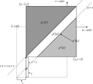
Figure (4.1) illustrates that summing terms of the form

(Bu+12nโˆ’1+sโˆ’Bu2nโˆ’1+s)โ€‹(Bv+12nโˆ’1+tโˆ’Bv2nโˆ’1+t)subscript๐ต๐‘ข1superscript2๐‘›1๐‘ subscript๐ต๐‘ขsuperscript2๐‘›1๐‘ subscript๐ต๐‘ฃ1superscript2๐‘›1๐‘กsubscript๐ต๐‘ฃsuperscript2๐‘›1๐‘ก\displaystyle\left(B_{\frac{u+1}{2^{n}}-1+s}-B_{\frac{u}{2^{n}}-1+s}\right)\left(B_{\frac{v+1}{2^{n}}-1+t}-B_{\frac{v}{2^{n}}-1+t}\right)
โˆ’(Bu+12nโˆ’1+tโˆ’Bu2nโˆ’1+t)โ€‹(Bv+12nโˆ’1+sโˆ’Bv2nโˆ’1+s)subscript๐ต๐‘ข1superscript2๐‘›1๐‘กsubscript๐ต๐‘ขsuperscript2๐‘›1๐‘กsubscript๐ต๐‘ฃ1superscript2๐‘›1๐‘ subscript๐ต๐‘ฃsuperscript2๐‘›1๐‘ \displaystyle-\left(B_{\frac{u+1}{2^{n}}-1+t}-B_{\frac{u}{2^{n}}-1+t}\right)\left(B_{\frac{v+1}{2^{n}}-1+s}-B_{\frac{v}{2^{n}}-1+s}\right)

over points $(\frac{u}{2^{n}},\frac{v}{2^{n}})$ in the upper dyadic triangle of the unit square as in (4.9), is equivalent to summing terms of the form

$$\left(B_{\frac{u+1}{2^{n}}}-B_{\frac{u}{2^{n}}}\right)\left(B_{\frac{v+1}{2^{n}}}-B_{\frac{v}{2^{n}}}\right)$$

over points $(\frac{u}{2^{n}},\frac{v}{2^{n}})$ in the upper dyadic triangle of the unit square shifted by (sโˆ’1,tโˆ’1)๐‘ 1๐‘ก1\left(s-1,t-1\right). This set of shifted points can be written as the (disjoint) union of

$\displaystyle\rho_{+}\left(n\right)$ $\displaystyle=$ $\displaystyle\left\{\left(\frac{u}{2^{n}},\frac{v}{2^{n}}\right):u,v\in\left\{0,1,2,...,2^{n}-1\right\}\text{ and}\right.$
u+12n+tโ‰คv2n+sโ€‹ย andย โ€‹u2nโ‰ฅsโˆ’1โ€‹ย andย ๐‘ข1superscript2๐‘›๐‘ก๐‘ฃsuperscript2๐‘›๐‘ ย andย ๐‘ขsuperscript2๐‘›๐‘ 1ย andย \displaystyle\left.\frac{u+1}{2^{n}}+t\leq\frac{v}{2^{n}}+s\text{ and }\frac{u}{2^{n}}\geq s-1\text{ and }\right.
$\displaystyle\left.t-1\leq\frac{v}{2^{n}}\leq t-\frac{1}{2^{n}}\right\},$
$\displaystyle\rho_{-}^{1}\left(n\right)$ $\displaystyle=$ $\displaystyle\left\{\left(\frac{u}{2^{n}},\frac{v}{2^{n}}\right):u,v\in\left\{0,1,2,...,2^{n}-1\right\}\text{ and}\right.$
u2n+tโ‰ฅv2n+sโ€‹ย andย โ€‹v2nโ‰ฅ(tโˆ’1)โˆจu+12n๐‘ขsuperscript2๐‘›๐‘ก๐‘ฃsuperscript2๐‘›๐‘ ย andย ๐‘ฃsuperscript2๐‘›๐‘ก1๐‘ข1superscript2๐‘›\displaystyle\left.\frac{u}{2^{n}}+t\geq\frac{v}{2^{n}}+s\text{ and }\frac{v}{2^{n}}\geq\left(t-1\right)\vee\frac{u+1}{2^{n}}\right.
$\displaystyle\left.\text{and }s-1\leq\frac{u}{2^{n}}\leq s-\frac{1}{2^{n}}\right\},$
$\displaystyle\rho_{-}^{2}\left(n\right)$ $\displaystyle=$ $\displaystyle\left\{\left(\frac{u}{2^{n}},\frac{v}{2^{n}}\right):u,v\in\left\{0,1,2,...,2^{n}-1\right\}\text{ and}\right.$
$\displaystyle\left.t-1\leq\frac{v}{2^{n}}\leq\frac{u-1}{2^{n}}\text{ and }t-1\leq\frac{u}{2^{n}}\leq s-\frac{1}{2^{n}}\right\}$

and

$\displaystyle\rho_{-}^{3}\left(n\right)$ $\displaystyle=$ $\displaystyle\left\{\left(\frac{u}{2^{n}},\frac{v}{2^{n}}\right):u,v\in\left\{0,1,2,...,2^{n}-1\right\}\text{ and}\right.$
$\displaystyle\left.u=v\text{ and }t-1\leq\frac{u}{2^{n}}\leq s-\frac{1}{2^{n}}\right\}.$

In this way, we can rewrite ๐’œ0,1โ€‹(๐’ฏBโ€‹(n))โ€‹(s,t)subscript๐’œ01superscript๐’ฏ๐ต๐‘›๐‘ ๐‘ก\mathcal{A}_{0,1}\left(\mathcal{T}^{B}\left(n\right)\right)\left(s,t\right) as

๐’œ0,1โ€‹(๐’ฏBโ€‹(n))โ€‹(s,t)subscript๐’œ01superscript๐’ฏ๐ต๐‘›๐‘ ๐‘ก\displaystyle\mathcal{A}_{0,1}\left(\mathcal{T}^{B}\left(n\right)\right)\left(s,t\right)
$\displaystyle=$ $\displaystyle\frac{1}{2}\sum_{\left(\frac{u}{2^{n}},\frac{v}{2^{n}}\right)\in\rho_{+}\left(n\right)}\left(B_{\frac{u+1}{2^{n}}}-B_{\frac{u}{2^{n}}}\right)\left(B_{\frac{v+1}{2^{n}}}-B_{\frac{v}{2^{n}}}\right)$
$\displaystyle-\frac{1}{2}\sum_{\left(\frac{u}{2^{n}},\frac{v}{2^{n}}\right)\in\rho_{-}^{1}\left(n\right)}\left(B_{\frac{u+1}{2^{n}}}-B_{\frac{u}{2^{n}}}\right)\left(B_{\frac{v+1}{2^{n}}}-B_{\frac{v}{2^{n}}}\right)$
$\displaystyle-\frac{1}{2}\sum_{\left(\frac{u}{2^{n}},\frac{v}{2^{n}}\right)\in\rho_{-}^{2}\left(n\right)}\left(B_{\frac{u+1}{2^{n}}}-B_{\frac{u}{2^{n}}}\right)\left(B_{\frac{v+1}{2^{n}}}-B_{\frac{v}{2^{n}}}\right)$
$\displaystyle-\frac{1}{2}\sum_{\left(\frac{u}{2^{n}},\frac{v}{2^{n}}\right)\in\rho_{-}^{3}\left(n\right)}\left(B_{\frac{u+1}{2^{n}}}-B_{\frac{u}{2^{n}}}\right)\left(B_{\frac{v+1}{2^{n}}}-B_{\frac{v}{2^{n}}}\right).$

Since t>s๐‘ก๐‘ t>s, the process $B_{.-\left(t-s\right)}$ is adapted to the Brownian filtration

$$\left\{\sigma\left(B_{u}:-1\leq u\leq t\right):t\in\left[-1,1\right]\right\}$$

and so

$\displaystyle\sum_{\left(\frac{u}{2^{n}},\frac{v}{2^{n}}\right)\in\rho_{+}\left(n\right)}\left(B_{\frac{u+1}{2^{n}}}-B_{\frac{u}{2^{n}}}\right)\left(B_{\frac{v+1}{2^{n}}}-B_{\frac{v}{2^{n}}}\right)$
$\displaystyle=$ โˆ‘v=2nโ€‹(tโˆ’1)2nโ€‹tโˆ’1(Bv2nโˆ’(tโˆ’s)โˆ’Bsโˆ’1)โ€‹(Bv+12nโˆ’Bv2n)superscriptsubscript๐‘ฃsuperscript2๐‘›๐‘ก1superscript2๐‘›๐‘ก1subscript๐ต๐‘ฃsuperscript2๐‘›๐‘ก๐‘ subscript๐ต๐‘ 1subscript๐ต๐‘ฃ1superscript2๐‘›subscript๐ต๐‘ฃsuperscript2๐‘›\displaystyle\sum_{v=2^{n}\left(t-1\right)}^{2^{n}t-1}\left(B_{\frac{v}{2^{n}}-\left(t-s\right)}-B_{s-1}\right)\left(B_{\frac{v+1}{2^{n}}}-B_{\frac{v}{2^{n}}}\right)

converges to the Itรด integral โˆซtโˆ’1t(Bvโˆ’(tโˆ’s)โˆ’Bsโˆ’1)โ€‹๐‘‘Bvsuperscriptsubscript๐‘ก1๐‘กsubscript๐ต๐‘ฃ๐‘ก๐‘ subscript๐ต๐‘ 1differential-dsubscript๐ต๐‘ฃ\int_{t-1}^{t}\left(B_{v-\left(t-s\right)}-B_{s-1}\right)dB_{v} as $n\rightarrow\infty$, $\mathbb{P}$-a.s.

Similarly,

$\displaystyle\sum_{\left(\frac{u}{2^{n}},\frac{v}{2^{n}}\right)\in\rho_{-}^{2}\left(n\right)}\left(B_{\frac{u+1}{2^{n}}}-B_{\frac{u}{2^{n}}}\right)\left(B_{\frac{v+1}{2^{n}}}-B_{\frac{v}{2^{n}}}\right)$
$\displaystyle=$ โˆ‘v=2nโ€‹(tโˆ’1)2nโ€‹sโˆ’1(Bv2nโˆ’Btโˆ’1)โ€‹(Bv+12nโˆ’Bv2n)superscriptsubscript๐‘ฃsuperscript2๐‘›๐‘ก1superscript2๐‘›๐‘ 1subscript๐ต๐‘ฃsuperscript2๐‘›subscript๐ต๐‘ก1subscript๐ต๐‘ฃ1superscript2๐‘›subscript๐ต๐‘ฃsuperscript2๐‘›\displaystyle\sum_{v=2^{n}\left(t-1\right)}^{2^{n}s-1}\left(B_{\frac{v}{2^{n}}}-B_{t-1}\right)\left(B_{\frac{v+1}{2^{n}}}-B_{\frac{v}{2^{n}}}\right)

converges to the Itรด integral โˆซtโˆ’1s(Bvโˆ’Btโˆ’1)โ€‹๐‘‘Bvsuperscriptsubscript๐‘ก1๐‘ subscript๐ต๐‘ฃsubscript๐ต๐‘ก1differential-dsubscript๐ต๐‘ฃ\int_{t-1}^{s}\left(B_{v}-B_{t-1}\right)dB_{v}, $\mathbb{P}$-a.s.

Furthermore, for ย the sum over $\rho_{-}^{3}\left(n\right)$, we get that

$\displaystyle\sum_{\left(\frac{u}{2^{n}},\frac{v}{2^{n}}\right)\in\rho_{-}^{3}\left(n\right)}\left(B_{\frac{u+1}{2^{n}}}-B_{\frac{u}{2^{n}}}\right)\left(B_{\frac{v+1}{2^{n}}}-B_{\frac{v}{2^{n}}}\right)$
$\displaystyle=$ โˆ‘u=(tโˆ’1)โ€‹2n2nโ€‹sโˆ’1(Bu+12nโˆ’Bu2n)2superscriptsubscript๐‘ข๐‘ก1superscript2๐‘›superscript2๐‘›๐‘ 1superscriptsubscript๐ต๐‘ข1superscript2๐‘›subscript๐ต๐‘ขsuperscript2๐‘›2\displaystyle\sum_{u=\left(t-1\right)2^{n}}^{2^{n}s-1}\left(B_{\frac{u+1}{2^{n}}}-B_{\frac{u}{2^{n}}}\right)^{2}

converges to the quadratic variation โŸจB,BโŸฉtโˆ’1s=1โˆ’t+ssuperscriptsubscript๐ต๐ต๐‘ก1๐‘ 1๐‘ก๐‘ \left\langle B,B\right\rangle_{t-1}^{s}=1-t+s , $\mathbb{P}$-a.s.

Finally, for the sum over $\rho_{-}^{1}\left(n\right),$ we find that

$\displaystyle\sum_{\left(\frac{u}{2^{n}},\frac{v}{2^{n}}\right)\in\rho_{-}^{1}\left(n\right)}\left(B_{\frac{u+1}{2^{n}}}-B_{\frac{u}{2^{n}}}\right)\left(B_{\frac{v+1}{2^{n}}}-B_{\frac{v}{2^{n}}}\right)$
$\displaystyle=$ โˆ‘v=2nโ€‹(sโˆ’1)2nโ€‹sโˆ’1(Bv+12n+tโˆ’sโˆ’B(tโˆ’1)โˆจv+12n)โ€‹(Bv+12nโˆ’Bv2n)superscriptsubscript๐‘ฃsuperscript2๐‘›๐‘ 1superscript2๐‘›๐‘ 1subscript๐ต๐‘ฃ1superscript2๐‘›๐‘ก๐‘ subscript๐ต๐‘ก1๐‘ฃ1superscript2๐‘›subscript๐ต๐‘ฃ1superscript2๐‘›subscript๐ต๐‘ฃsuperscript2๐‘›\displaystyle\sum_{v=2^{n}\left(s-1\right)}^{2^{n}s-1}\left(B_{\frac{v+1}{2^{n}}+t-s}-B_{\left(t-1\right)\vee\frac{v+1}{2^{n}}}\right)\left(B_{\frac{v+1}{2^{n}}}-B_{\frac{v}{2^{n}}}\right)
$\displaystyle=$ โˆ‘k=2nโ€‹(1โˆ’s)+12nโ€‹(2โˆ’s)(B1โˆ’kโˆ’12n+(tโˆ’s)โˆ’B(tโˆ’1)โˆจ1โˆ’kโˆ’12n)โ€‹(B1โˆ’kโˆ’12nโˆ’B1โˆ’k2n)superscriptsubscript๐‘˜superscript2๐‘›1๐‘ 1superscript2๐‘›2๐‘ subscript๐ต1๐‘˜1superscript2๐‘›๐‘ก๐‘ subscript๐ต๐‘ก11๐‘˜1superscript2๐‘›subscript๐ต1๐‘˜1superscript2๐‘›subscript๐ต1๐‘˜superscript2๐‘›\displaystyle\sum_{k=2^{n}\left(1-s\right)+1}^{2^{n}\left(2-s\right)}\left(B_{1-\frac{k-1}{2^{n}}+\left(t-s\right)}-B_{\left(t-1\right)\vee 1-\frac{k-1}{2^{n}}}\right)\left(B_{1-\frac{k-1}{2^{n}}}-B_{1-\frac{k}{2^{n}}}\right)
$\displaystyle=$ โˆ‘k=2nโ€‹(1โˆ’s)+12nโ€‹(2โˆ’s)[(B1โˆ’B(tโˆ’1)โˆจ1โˆ’kโˆ’12n)โˆ’(B1โˆ’B1โˆ’kโˆ’12n+(tโˆ’s))]superscriptsubscript๐‘˜superscript2๐‘›1๐‘ 1superscript2๐‘›2๐‘ delimited-[]subscript๐ต1subscript๐ต๐‘ก11๐‘˜1superscript2๐‘›subscript๐ต1subscript๐ต1๐‘˜1superscript2๐‘›๐‘ก๐‘ \displaystyle\sum_{k=2^{n}\left(1-s\right)+1}^{2^{n}\left(2-s\right)}\left[\left(B_{1}-B_{\left(t-1\right)\vee 1-\frac{k-1}{2^{n}}}\right)-\left(B_{1}-B_{1-\frac{k-1}{2^{n}}+\left(t-s\right)}\right)\right]
$\displaystyle\times\left[\left(B_{1}-B_{1-\frac{k}{2^{n}}}\right)-\left(B_{1}-B_{1-\frac{k-1}{2^{n}}}\right)\right]$
$\displaystyle=$ โˆ‘k=2nโ€‹(1โˆ’s)+12nโ€‹(2โˆ’s)(B^2โˆ’tโˆงkโˆ’12nโˆ’B^kโˆ’12nโˆ’(tโˆ’s))โ€‹(B^k2nโˆ’B^kโˆ’12n)superscriptsubscript๐‘˜superscript2๐‘›1๐‘ 1superscript2๐‘›2๐‘ subscript^๐ต2๐‘ก๐‘˜1superscript2๐‘›subscript^๐ต๐‘˜1superscript2๐‘›๐‘ก๐‘ subscript^๐ต๐‘˜superscript2๐‘›subscript^๐ต๐‘˜1superscript2๐‘›\displaystyle\sum_{k=2^{n}\left(1-s\right)+1}^{2^{n}\left(2-s\right)}\left(\hat{B}_{2-t\wedge\frac{k-1}{2^{n}}}-\hat{B}_{\frac{k-1}{2^{n}}-\left(t-s\right)}\right)\left(\hat{B}_{\frac{k}{2^{n}}}-\hat{B}_{\frac{k-1}{2^{n}}}\right)

where $\hat{B}_{u}:=B_{1}-B_{1-u}$ is a Brownian motion with respect to the filtration

$$\left\{\sigma\left(\hat{B}_{u}:0\leq u\leq t\right):t\in\left[0,2\right]\right\}.$$

Taking the limit as $n\rightarrow\infty$, we find that

โˆ‘k=2nโ€‹(1โˆ’s)+12nโ€‹(2โˆ’s)(B^2โˆ’tโˆงkโˆ’12nโˆ’B^kโˆ’12nโˆ’(tโˆ’s))โ€‹(B^k2nโˆ’B^kโˆ’12n)superscriptsubscript๐‘˜superscript2๐‘›1๐‘ 1superscript2๐‘›2๐‘ subscript^๐ต2๐‘ก๐‘˜1superscript2๐‘›subscript^๐ต๐‘˜1superscript2๐‘›๐‘ก๐‘ subscript^๐ต๐‘˜superscript2๐‘›subscript^๐ต๐‘˜1superscript2๐‘›\displaystyle\sum_{k=2^{n}\left(1-s\right)+1}^{2^{n}\left(2-s\right)}\left(\hat{B}_{2-t\wedge\frac{k-1}{2^{n}}}-\hat{B}_{\frac{k-1}{2^{n}}-\left(t-s\right)}\right)\left(\hat{B}_{\frac{k}{2^{n}}}-\hat{B}_{\frac{k-1}{2^{n}}}\right)
$\displaystyle\rightarrow$ โˆซ1โˆ’s2โˆ’tB^uโ€‹๐‘‘B^u+B^2โˆ’tโ€‹(B^2โˆ’sโˆ’B^2โˆ’t)โˆ’โˆซ1โˆ’s2โˆ’sB^uโˆ’(tโˆ’s)โ€‹๐‘‘B^usuperscriptsubscript1๐‘ 2๐‘กsubscript^๐ต๐‘ขdifferential-dsubscript^๐ต๐‘ขsubscript^๐ต2๐‘กsubscript^๐ต2๐‘ subscript^๐ต2๐‘กsuperscriptsubscript1๐‘ 2๐‘ subscript^๐ต๐‘ข๐‘ก๐‘ differential-dsubscript^๐ต๐‘ข\displaystyle\int_{1-s}^{2-t}\hat{B}_{u}d\hat{B}_{u}+\hat{B}_{2-t}\left(\hat{B}_{2-s}-\hat{B}_{2-t}\right)-\int_{1-s}^{2-s}\hat{B}_{u-\left(t-s\right)}d\hat{B}_{u}

After some tidying up, we find that for dyadic times s<t๐‘ ๐‘กs<t,

๐’œ0,1โ€‹(๐’ฏB)โ€‹(s,t)subscript๐’œ01superscript๐’ฏ๐ต๐‘ ๐‘ก\displaystyle\mathcal{A}_{0,1}\left(\mathcal{T}^{B}\right)\left(s,t\right)
$\displaystyle=$ 12โ€‹โˆซtโˆ’1tBvโˆ’(tโˆ’s)โ€‹๐‘‘Bvโˆ’12โ€‹Bsโˆ’1โ€‹(Btโˆ’Btโˆ’1)โˆ’12โ€‹โˆซtโˆ’1sBvโ€‹๐‘‘Bv+12โ€‹Btโˆ’1โ€‹(Bsโˆ’Btโˆ’1)12superscriptsubscript๐‘ก1๐‘กsubscript๐ต๐‘ฃ๐‘ก๐‘ differential-dsubscript๐ต๐‘ฃ12subscript๐ต๐‘ 1subscript๐ต๐‘กsubscript๐ต๐‘ก112superscriptsubscript๐‘ก1๐‘ subscript๐ต๐‘ฃdifferential-dsubscript๐ต๐‘ฃ12subscript๐ต๐‘ก1subscript๐ต๐‘ subscript๐ต๐‘ก1\displaystyle\frac{1}{2}\int_{t-1}^{t}B_{v-\left(t-s\right)}dB_{v}-\frac{1}{2}B_{s-1}\left(B_{t}-B_{t-1}\right)-\frac{1}{2}\int_{t-1}^{s}B_{v}dB_{v}+\frac{1}{2}B_{t-1}\left(B_{s}-B_{t-1}\right)
โˆ’12โ€‹(1โˆ’t+s)121๐‘ก๐‘ \displaystyle-\frac{1}{2}\left(1-t+s\right)
+12โ€‹โˆซ1โˆ’s2โˆ’sB^vโˆ’(tโˆ’s)โ€‹๐‘‘B^vโˆ’12โ€‹โˆซ1โˆ’s2โˆ’tB^vโ€‹๐‘‘B^vโˆ’12โ€‹B^2โˆ’tโ€‹(B^2โˆ’sโˆ’B^2โˆ’t).12superscriptsubscript1๐‘ 2๐‘ subscript^๐ต๐‘ฃ๐‘ก๐‘ differential-dsubscript^๐ต๐‘ฃ12superscriptsubscript1๐‘ 2๐‘กsubscript^๐ต๐‘ฃdifferential-dsubscript^๐ต๐‘ฃ12subscript^๐ต2๐‘กsubscript^๐ต2๐‘ subscript^๐ต2๐‘ก\displaystyle+\frac{1}{2}\int_{1-s}^{2-s}\hat{B}_{v-\left(t-s\right)}d\hat{B}_{v}-\frac{1}{2}\int_{1-s}^{2-t}\hat{B}_{v}d\hat{B}_{v}-\frac{1}{2}\hat{B}_{2-t}\left(\hat{B}_{2-s}-\hat{B}_{2-t}\right).

4.5.3 Non-existence of the Lรฉvy area random variable $\mathcal{A}_{0,1}\left(\mathcal{T}^{B}\right)$ in the injective tensor product

In Proposition 4.5.67, we showed that $\mathcal{A}_{0,1}\left(\mathcal{T}^{B}\right)$ exists on the dyadic unit square $D\left(\left[0,1\right]^{2}\right)$. In this section, we prove that $\mathcal{A}_{0,1}\left(\mathcal{T}^{B}\right)$ has a unique continuous extension to the entire unit square excluding the diagonal. We show that this extension has a jump discontinuity on the diagonal and hence, that the Lรฉvy area does not exist in the injectiveย tensor product.

Proposition 4.5.69.

With $\mathbb{P}$-probability $1$, the Lรฉvy Area $\mathcal{A}_{0,1}\left(\mathcal{T}^{B}\right)$ as defined in Proposition 4.5.67 on the dyadic open upper triangle

{(s,t)โˆˆDโ€‹([0,1]2):0โ‰คs<tโ‰ค1}conditional-set๐‘ ๐‘ก๐ทsuperscript0120๐‘ ๐‘ก1\left\{\left(s,t\right)\in D\left(\left[0,1\right]^{2}\right):0\leq s<t\leq 1\right\}

has a unique uniformly continuous extension $\mathcal{A}_{0,1}^{\ast}\left(\mathcal{T}^{B}\right)$ to the open upper triangle

{(s,t)โˆˆ[0,1]ร—[0,1]:0โ‰คs<tโ‰ค1}conditional-set๐‘ ๐‘ก01010๐‘ ๐‘ก1\left\{\left(s,t\right)\in\left[0,1\right]\times\left[0,1\right]:0\leq s<t\leq 1\right\}

and hence by (4.7) to the open lower triangle of the unit square

{(s,t)โˆˆ[0,1]ร—[0,1]:0โ‰คt<sโ‰ค1}.conditional-set๐‘ ๐‘ก01010๐‘ก๐‘ 1\left\{\left(s,t\right)\in\left[0,1\right]\times\left[0,1\right]:0\leq t<s\leq 1\right\}.

$\mathcal{A}_{0,1}^{\ast}\left(\mathcal{T}^{B}\right)$ agrees with $\mathcal{A}_{0,1}\left(\mathcal{T}^{B}\right)$ on the dyadic open upper triangle (dyadic open lower triangle) on a set $\Omega_{0}$ of full $\mathbb{P}$-measure.

$\mathcal{A}_{0,1}^{\ast}\left(\mathcal{T}^{B}\right)$ has a jump discontinuity on the diagonal and so does not exist in the injective tensor algebra $C\left(\left[0,1\right]\times\left[0,1\right]\right)$ (c.f. Proposition 4.3.61): There does not exist a continuous extension of $\mathcal{A}_{0,1}$ to the unit square.

Proof 4.5.70.

We start by proving the existence of a continuous extension of $\mathcal{A}_{0,1}\left(\mathcal{T}^{B}\right)$ to the open upper triangle:ย In Proposition 4.5.67, we showed that on the open upper dyadic triangle,

{(s,t)โˆˆDโ€‹([0,1]2):0โ‰คs<tโ‰ค1},conditional-set๐‘ ๐‘ก๐ทsuperscript0120๐‘ ๐‘ก1\left\{\left(s,t\right)\in D\left(\left[0,1\right]^{2}\right):0\leq s<t\leq 1\right\},

๐’œ0,1โ€‹(๐’ฏB)โ€‹(s,t)subscript๐’œ01superscript๐’ฏ๐ต๐‘ ๐‘ก\mathcal{A}_{0,1}\left(\mathcal{T}^{B}\right)\left(s,t\right) has the following representation:

๐’œ0,1โ€‹(๐’ฏB)โ€‹(s,t)subscript๐’œ01superscript๐’ฏ๐ต๐‘ ๐‘ก\displaystyle\mathcal{A}_{0,1}\left(\mathcal{T}^{B}\right)\left(s,t\right) (4.10)
$\displaystyle=$ 12โ€‹โˆซtโˆ’1tBvโˆ’(tโˆ’s)โ€‹๐‘‘Bvโˆ’12โ€‹โˆซtโˆ’1sBvโ€‹๐‘‘Bv+12โ€‹Btโˆ’1โ€‹(Bsโˆ’Btโˆ’1)โˆ’12โ€‹Bsโˆ’1โ€‹(Btโˆ’Btโˆ’1)12superscriptsubscript๐‘ก1๐‘กsubscript๐ต๐‘ฃ๐‘ก๐‘ differential-dsubscript๐ต๐‘ฃ12superscriptsubscript๐‘ก1๐‘ subscript๐ต๐‘ฃdifferential-dsubscript๐ต๐‘ฃ12subscript๐ต๐‘ก1subscript๐ต๐‘ subscript๐ต๐‘ก112subscript๐ต๐‘ 1subscript๐ต๐‘กsubscript๐ต๐‘ก1\displaystyle\frac{1}{2}\int_{t-1}^{t}B_{v-\left(t-s\right)}dB_{v}-\frac{1}{2}\int_{t-1}^{s}B_{v}dB_{v}+\frac{1}{2}B_{t-1}\left(B_{s}-B_{t-1}\right)-\frac{1}{2}B_{s-1}\left(B_{t}-B_{t-1}\right)
โˆ’12โ€‹(1โˆ’t+s)121๐‘ก๐‘ \displaystyle-\frac{1}{2}\left(1-t+s\right)
+12โ€‹โˆซ1โˆ’s2โˆ’sB^vโˆ’(tโˆ’s)โ€‹๐‘‘B^vโˆ’12โ€‹โˆซ1โˆ’s2โˆ’tB^vโ€‹๐‘‘B^vโˆ’12โ€‹B^2โˆ’tโ€‹(B^2โˆ’sโˆ’B^2โˆ’t).12superscriptsubscript1๐‘ 2๐‘ subscript^๐ต๐‘ฃ๐‘ก๐‘ differential-dsubscript^๐ต๐‘ฃ12superscriptsubscript1๐‘ 2๐‘กsubscript^๐ต๐‘ฃdifferential-dsubscript^๐ต๐‘ฃ12subscript^๐ต2๐‘กsubscript^๐ต2๐‘ subscript^๐ต2๐‘ก\displaystyle+\frac{1}{2}\int_{1-s}^{2-s}\hat{B}_{v-\left(t-s\right)}d\hat{B}_{v}-\frac{1}{2}\int_{1-s}^{2-t}\hat{B}_{v}d\hat{B}_{v}-\frac{1}{2}\hat{B}_{2-t}\left(\hat{B}_{2-s}-\hat{B}_{2-t}\right).

For a Brownian Motion $W$, the Itรด integral Mb:=โˆซcโ€‹oโ€‹nโ€‹sโ€‹tbWuโ€‹๐‘‘Wuassignsubscript๐‘€๐‘superscriptsubscript๐‘๐‘œ๐‘›๐‘ ๐‘ก๐‘subscript๐‘Š๐‘ขdifferential-dsubscript๐‘Š๐‘ขM_{b}:=\int_{const}^{b}W_{u}dW_{u} is a continuous martingale with respect to the filtration $\left\{\sigma\left(W_{u}:const\leq u\leq b\right):b\in\left[const,T\right]\right\}$, so that $M\left(a,b\right):=M\left(b\right)-M\left(a\right)$ is continuous on a set of full $\mathbb{P}$-measure. Furthermore, the closed upper triangle

{(s,t)โˆˆ[0,1]ร—[0,1]:0โ‰คsโ‰คtโ‰ค1}conditional-set๐‘ ๐‘ก01010๐‘ ๐‘ก1\left\{\left(s,t\right)\in\left[0,1\right]\times\left[0,1\right]:0\leq s\leq t\leq 1\right\}

is compact. Hence,

F1โ€‹(s,t):=12โ€‹โˆซtโˆ’1sBvโ€‹๐‘‘Bvassignsubscript๐น1๐‘ ๐‘ก12superscriptsubscript๐‘ก1๐‘ subscript๐ต๐‘ฃdifferential-dsubscript๐ต๐‘ฃF_{1}\left(s,t\right):=\frac{1}{2}\int_{t-1}^{s}B_{v}dB_{v}

and

F^1โ€‹(s,t):=12โ€‹โˆซ1โˆ’s2โˆ’tB^vโ€‹๐‘‘B^vassignsubscript^๐น1๐‘ ๐‘ก12superscriptsubscript1๐‘ 2๐‘กsubscript^๐ต๐‘ฃdifferential-dsubscript^๐ต๐‘ฃ\hat{F}_{1}\left(s,t\right):=\frac{1}{2}\int_{1-s}^{2-t}\hat{B}_{v}d\hat{B}_{v}

have uniformly continuous sample paths on the closed upper triangle. Btโˆ’1โ€‹(Bsโˆ’Btโˆ’1)subscript๐ต๐‘ก1subscript๐ต๐‘ subscript๐ต๐‘ก1B_{t-1}\left(B_{s}-B_{t-1}\right), Bsโˆ’1โ€‹(Btโˆ’Btโˆ’1)subscript๐ต๐‘ 1subscript๐ต๐‘กsubscript๐ต๐‘ก1B_{s-1}\left(B_{t}-B_{t-1}\right) and B^2โˆ’tโ€‹(B^2โˆ’sโˆ’B^2โˆ’t)subscript^๐ต2๐‘กsubscript^๐ต2๐‘ subscript^๐ต2๐‘ก\hat{B}_{2-t}\left(\hat{B}_{2-s}-\hat{B}_{2-t}\right) are uniformly continuous in s๐‘ s and $t$ ย on the closed upper triangle because of the $\mathbb{P}$-a.s. sample path continuity of Brownian motion and compactness of the closed upper triangle. This leaves us with having to prove that the terms

F2โ€‹(s,t):=โˆซtโˆ’1tBvโˆ’(tโˆ’s)โ€‹๐‘‘Bvassignsubscript๐น2๐‘ ๐‘กsuperscriptsubscript๐‘ก1๐‘กsubscript๐ต๐‘ฃ๐‘ก๐‘ differential-dsubscript๐ต๐‘ฃF_{2}\left(s,t\right):=\int_{t-1}^{t}B_{v-\left(t-s\right)}dB_{v}

and

F^2โ€‹(s,t):=โˆซ1โˆ’s2โˆ’sB^uโˆ’(tโˆ’s)โ€‹๐‘‘B^uassignsubscript^๐น2๐‘ ๐‘กsuperscriptsubscript1๐‘ 2๐‘ subscript^๐ต๐‘ข๐‘ก๐‘ differential-dsubscript^๐ต๐‘ข\hat{F}_{2}\left(s,t\right):=\int_{1-s}^{2-s}\hat{B}_{u-\left(t-s\right)}d\hat{B}_{u}

have uniformly continuous modifications on the closed dyadic upper triangle. Since

{(s,t)โˆˆDโ€‹([0,1]2):0โ‰คsโ‰คtโ‰ค1}conditional-set๐‘ ๐‘ก๐ทsuperscript0120๐‘ ๐‘ก1\left\{\left(s,t\right)\in D\left(\left[0,1\right]^{2}\right):0\leq s\leq t\leq 1\right\}

is dense in

{(s,t)โˆˆ[0,1]ร—[0,1]:0โ‰คsโ‰คtโ‰ค1},conditional-set๐‘ ๐‘ก01010๐‘ ๐‘ก1\left\{\left(s,t\right)\in\left[0,1\right]\times\left[0,1\right]:0\leq s\leq t\leq 1\right\},

this is equivalent to showing that $F_{2}$ and $\hat{F}_{2}$ each have a unique uniformly continuous extension to the closed upper triangle.

We start by establishing the existence of a continuous modification of $F_{2}$ by using Kolmogorovโ€™s Lemma (Theorem 2.4.35 in Chapter $2$) for a two-dimensional parameter set. Suppose that (s1,t1)subscript๐‘ 1subscript๐‘ก1\left(s_{1},t_{1}\right) and (s2,t2)subscript๐‘ 2subscript๐‘ก2\left(s_{2},t_{2}\right) are in {(s,t)โˆˆDโ€‹([0,1]2):0โ‰คs<tโ‰ค1}conditional-set๐‘ ๐‘ก๐ทsuperscript0120๐‘ ๐‘ก1\left\{\left(s,t\right)\in D\left(\left[0,1\right]^{2}\right):0\leq s<t\leq 1\right\} and w.l.o.g. suppose that $t_{2}\geq t_{1}$. For $m\in\mathbb{N}$, we have that

|F2โ€‹(s2,t2)โˆ’F2โ€‹(s1,t1)|2โ€‹msuperscriptsubscript๐น2subscript๐‘ 2subscript๐‘ก2subscript๐น2subscript๐‘ 1subscript๐‘ก12๐‘š\displaystyle\left|F_{2}\left(s_{2},t_{2}\right)-F_{2}\left(s_{1},t_{1}\right)\right|^{2m}
$\displaystyle=$ |F2โ€‹(s2,t2)โˆ’F2โ€‹(s1,t2)+F2โ€‹(s1,t2)โˆ’F2โ€‹(s1,t1)|2โ€‹msuperscriptsubscript๐น2subscript๐‘ 2subscript๐‘ก2subscript๐น2subscript๐‘ 1subscript๐‘ก2subscript๐น2subscript๐‘ 1subscript๐‘ก2subscript๐น2subscript๐‘ 1subscript๐‘ก12๐‘š\displaystyle\left|F_{2}\left(s_{2},t_{2}\right)-F_{2}\left(s_{1},t_{2}\right)+F_{2}\left(s_{1},t_{2}\right)-F_{2}\left(s_{1},t_{1}\right)\right|^{2m}
$\displaystyle\leq$ $\displaystyle 4^{2m-1}\left\{\left|\int_{t_{2}-1}^{t_{2}}\left(B_{u-\left(t_{2}-s_{2}\right)}-B_{u-\left(t_{2}-s_{1}\right)}\right)dB_{u}\right|^{2m}+\left|\int_{t_{1}}^{t_{2}}B_{u-\left(t_{2}-s_{1}\right)}dB_{u}\right|^{2m}\right.$
$\displaystyle\left.+\left|\int_{t_{2}-1}^{t_{1}}\left(B_{u-\left(t_{2}-s_{1}\right)}-B_{u-\left(t_{1}-s_{1}\right)}\right)dB_{u}\right|^{2m}+\left|\int_{t_{1}-1}^{t_{2}-1}B_{u-\left(t_{1}-s_{1}\right)}dB_{u}\right|^{2m}\right\}$

by Jensenโ€™s inequality. We require the following result from [Karatzas and Shreve, 1991], equations (3.24) and (3.25): If $X$ is a measurable, adapted process satisfying

$$\mathbb{E}\left[\int_{0}^{T}X_{t}^{2m}dt\right]<\infty,$$

for some real number $T>0$ and $m\in\mathbb{N}$ and $W_{.}$ is a standard, one-dimensional Brownian Motion on $\left[0,T\right]$, then

$$\mathbb{E}\left[\left|\int_{0}^{T}X_{u}dW_{u}\right|^{2m}\right]\leq\left(m\left(2m-1\right)\right)^{m}T^{m-1}\mathbb{E}\left[\int_{0}^{T}\left|X_{u}\right|^{2m}du\right].$$

We apply this to our setup where the Brownian motion $B$ is defined on $\left[-1,1\right]$ ( instead of on $\left[0,T\right]$ ) to find the following moment bounds: We find that

๐”ผโ€‹[|โˆซt2โˆ’1t2(Buโˆ’(t2โˆ’s2)โˆ’Buโˆ’(t2โˆ’s1))โ€‹๐‘‘Bu|2โ€‹m]๐”ผdelimited-[]superscriptsuperscriptsubscriptsubscript๐‘ก21subscript๐‘ก2subscript๐ต๐‘ขsubscript๐‘ก2subscript๐‘ 2subscript๐ต๐‘ขsubscript๐‘ก2subscript๐‘ 1differential-dsubscript๐ต๐‘ข2๐‘š\displaystyle\mathbb{E}\left[\left|\int_{t_{2}-1}^{t_{2}}\left(B_{u-\left(t_{2}-s_{2}\right)}-B_{u-\left(t_{2}-s_{1}\right)}\right)dB_{u}\right|^{2m}\right]
$\displaystyle\leq$ (mโ€‹(2โ€‹mโˆ’1))mโ€‹2mฯ€โ€‹ฮ“โ€‹(2โ€‹m+12)โ€‹|s2โˆ’s1|m,superscript๐‘š2๐‘š1๐‘šsuperscript2๐‘š๐œ‹ฮ“2๐‘š12superscriptsubscript๐‘ 2subscript๐‘ 1๐‘š\displaystyle\left(m\left(2m-1\right)\right)^{m}\frac{2^{m}}{\sqrt{\pi}}\Gamma\left(\frac{2m+1}{2}\right)\left|s_{2}-s_{1}\right|^{m},

where we used (2.11) in Chapter 2. Similarly, we find that

๐”ผโ€‹[|โˆซt1t2Buโˆ’(t2โˆ’s1)โ€‹๐‘‘Bu|2โ€‹m]๐”ผdelimited-[]superscriptsuperscriptsubscriptsubscript๐‘ก1subscript๐‘ก2subscript๐ต๐‘ขsubscript๐‘ก2subscript๐‘ 1differential-dsubscript๐ต๐‘ข2๐‘š\displaystyle\mathbb{E}\left[\left|\int_{t_{1}}^{t_{2}}B_{u-\left(t_{2}-s_{1}\right)}dB_{u}\right|^{2m}\right]
$\displaystyle\leq$ (mโ€‹(2โ€‹mโˆ’1))mโ€‹2mฯ€โ€‹ฮ“โ€‹(2โ€‹m+12)โ€‹|t2โˆ’t1|mโˆ’1โ€‹โˆซt1t2|uโˆ’t2+s1|mโ€‹๐‘‘usuperscript๐‘š2๐‘š1๐‘šsuperscript2๐‘š๐œ‹ฮ“2๐‘š12superscriptsubscript๐‘ก2subscript๐‘ก1๐‘š1superscriptsubscriptsubscript๐‘ก1subscript๐‘ก2superscript๐‘ขsubscript๐‘ก2subscript๐‘ 1๐‘šdifferential-d๐‘ข\displaystyle\left(m\left(2m-1\right)\right)^{m}\frac{2^{m}}{\sqrt{\pi}}\Gamma\left(\frac{2m+1}{2}\right)\left|t_{2}-t_{1}\right|^{m-1}\int_{t_{1}}^{t_{2}}\left|u-t_{2}+s_{1}\right|^{m}du
$\displaystyle\leq$ $\displaystyle\left(m\left(2m-1\right)\right)^{m}\frac{2^{m}}{\sqrt{\pi}}\Gamma\left(\frac{2m+1}{2}\right)\left|t_{2}-t_{1}\right|^{m},$

and

๐”ผโ€‹[|โˆซt2โˆ’1t1(Buโˆ’(t2โˆ’s1)โˆ’Buโˆ’(t1โˆ’s1))โ€‹๐‘‘Bu|2โ€‹m]๐”ผdelimited-[]superscriptsuperscriptsubscriptsubscript๐‘ก21subscript๐‘ก1subscript๐ต๐‘ขsubscript๐‘ก2subscript๐‘ 1subscript๐ต๐‘ขsubscript๐‘ก1subscript๐‘ 1differential-dsubscript๐ต๐‘ข2๐‘š\displaystyle\mathbb{E}\left[\left|\int_{t_{2}-1}^{t_{1}}\left(B_{u-\left(t_{2}-s_{1}\right)}-B_{u-\left(t_{1}-s_{1}\right)}\right)dB_{u}\right|^{2m}\right]
$\displaystyle\leq$ $\displaystyle\left(m\left(2m-1\right)\right)^{m}\frac{2^{m}}{\sqrt{\pi}}\Gamma\left(\frac{2m+1}{2}\right)\left|t_{2}-t_{1}\right|^{m},$

and finally that

๐”ผโ€‹[|โˆซt1โˆ’1t2โˆ’1Buโˆ’(t1โˆ’s1)โ€‹๐‘‘Bu|2โ€‹m]๐”ผdelimited-[]superscriptsuperscriptsubscriptsubscript๐‘ก11subscript๐‘ก21subscript๐ต๐‘ขsubscript๐‘ก1subscript๐‘ 1differential-dsubscript๐ต๐‘ข2๐‘š\displaystyle\mathbb{E}\left[\left|\int_{t_{1}-1}^{t_{2}-1}B_{u-\left(t_{1}-s_{1}\right)}dB_{u}\right|^{2m}\right]
$\displaystyle\leq$ $\displaystyle\left(m\left(2m-1\right)\right)^{m}\frac{2^{m}}{\sqrt{\pi}}\Gamma\left(\frac{2m+1}{2}\right)\left|t_{2}-t_{1}\right|^{m}.$

Therefore, for $m=3$, we have the bound

๐”ผโ€‹[|F2โ€‹(s2,t2)โˆ’F2โ€‹(s1,t1)|6]โ‰ค153โ€‹.215ฯ€โ€‹ฮ“โ€‹(72)โ€‹(maxโก(|s2โˆ’s1|,|t2โˆ’t1|))3.๐”ผdelimited-[]superscriptsubscript๐น2subscript๐‘ 2subscript๐‘ก2subscript๐น2subscript๐‘ 1subscript๐‘ก16superscript153superscript.215๐œ‹ฮ“72superscriptsubscript๐‘ 2subscript๐‘ 1subscript๐‘ก2subscript๐‘ก13\mathbb{E}\left[\left|F_{2}\left(s_{2},t_{2}\right)-F_{2}\left(s_{1},t_{1}\right)\right|^{6}\right]\leq\frac{15^{3}.2^{15}}{\sqrt{\pi}}\Gamma\left(\frac{7}{2}\right)\left(\max\left(\left|s_{2}-s_{1}\right|,\left|t_{2}-t_{1}\right|\right)\right)^{3}.

Hence, by Kolmogorovโ€™s Theorem (c.f. Theorem 2.4.35ย in Chapter 2), $F_{2}\left(.,.\right)$ has a continuous modification $F_{2}^{\ast}$ on the closed upper dyadic triangle

{(s,t)โˆˆDโ€‹([0,1]2):0โ‰คsโ‰คtโ‰ค1}.conditional-set๐‘ ๐‘ก๐ทsuperscript0120๐‘ ๐‘ก1\left\{\left(s,t\right)\in D\left(\left[0,1\right]^{2}\right):0\leq s\leq t\leq 1\right\}.

Since the closed upper dyadic triangle is dense in the closed upper triangle

{(s,t):0โ‰คsโ‰คtโ‰ค1},conditional-set๐‘ ๐‘ก0๐‘ ๐‘ก1\left\{\left(s,t\right):0\leq s\leq t\leq 1\right\},

$F_{2}^{\ast}$ has a unique uniformly continuous extension $G_{2}^{\ast}$ to the closed upper triangle.

The argument for $\hat{F}_{2}$ is similar โ€“ its continuous extension to the closed upper triangle is denoted as $\hat{G}_{2}^{\ast}$.

In summary,

๐’œ0,1โˆ—โ€‹(๐’ฏB)โ€‹(s,t):=12โ€‹G2โˆ—โ€‹(s,t)โˆ’12โ€‹โˆซtโˆ’1sBvโ€‹๐‘‘Bvassignsuperscriptsubscript๐’œ01โˆ—superscript๐’ฏ๐ต๐‘ ๐‘ก12superscriptsubscript๐บ2โˆ—๐‘ ๐‘ก12superscriptsubscript๐‘ก1๐‘ subscript๐ต๐‘ฃdifferential-dsubscript๐ต๐‘ฃ\displaystyle\mathcal{A}_{0,1}^{\ast}\left(\mathcal{T}^{B}\right)\left(s,t\right):=\frac{1}{2}G_{2}^{\ast}\left(s,t\right)-\frac{1}{2}\int_{t-1}^{s}B_{v}dB_{v}
+12โ€‹Btโˆ’1โ€‹(Bsโˆ’Btโˆ’1)โˆ’12โ€‹Bsโˆ’1โ€‹(Btโˆ’Btโˆ’1)12subscript๐ต๐‘ก1subscript๐ต๐‘ subscript๐ต๐‘ก112subscript๐ต๐‘ 1subscript๐ต๐‘กsubscript๐ต๐‘ก1\displaystyle+\frac{1}{2}B_{t-1}\left(B_{s}-B_{t-1}\right)-\frac{1}{2}B_{s-1}\left(B_{t}-B_{t-1}\right)
โˆ’12โ€‹(1โˆ’t+s)121๐‘ก๐‘ \displaystyle-\frac{1}{2}\left(1-t+s\right)
+12โ€‹G^2โˆ—โ€‹(s,t)โˆ’12โ€‹โˆซ1โˆ’s2โˆ’tB^vโ€‹๐‘‘B^vโˆ’12โ€‹B^2โˆ’tโ€‹(B^2โˆ’sโˆ’B^2โˆ’t),12superscriptsubscript^๐บ2โˆ—๐‘ ๐‘ก12superscriptsubscript1๐‘ 2๐‘กsubscript^๐ต๐‘ฃdifferential-dsubscript^๐ต๐‘ฃ12subscript^๐ต2๐‘กsubscript^๐ต2๐‘ subscript^๐ต2๐‘ก\displaystyle+\frac{1}{2}\hat{G}_{2}^{\ast}\left(s,t\right)-\frac{1}{2}\int_{1-s}^{2-t}\hat{B}_{v}d\hat{B}_{v}-\frac{1}{2}\hat{B}_{2-t}\left(\hat{B}_{2-s}-\hat{B}_{2-t}\right), (4.11)

is $\mathbb{P}$-a.s. uniformly continuous on the closed upper triangle

{(s,t)โˆˆ[0,1]ร—[0,1]:0โ‰คsโ‰คtโ‰ค1}.conditional-set๐‘ ๐‘ก01010๐‘ ๐‘ก1\left\{\left(s,t\right)\in\left[0,1\right]\times\left[0,1\right]:0\leq s\leq t\leq 1\right\}.

The restriction of $\mathcal{A}_{0,1}^{\ast}\left(\mathcal{T}^{B}\right)$ to the dyadic open upper triangle

{(s,t)โˆˆD2โ€‹([0,1]2):0โ‰คs<tโ‰ค1}conditional-set๐‘ ๐‘กsuperscript๐ท2superscript0120๐‘ ๐‘ก1\left\{\left(s,t\right)\in D^{2}\left(\left[0,1\right]^{2}\right):0\leq s<t\leq 1\right\}

agrees with $\mathcal{A}_{0,1}\left(\mathcal{T}^{B}\right)$ on a set $\Omega_{0}$ of full $\mathbb{P}$-measure.

To see that $\mathcal{A}_{0,1}^{\ast}\left(\mathcal{T}^{B}\right)$ has a jump discontinuity on the diagonal suppose that $u_{n}\nearrow u$ such that

(un,u)โˆˆ{(s,t)โˆˆ[0,1]ร—[0,1]:0โ‰คs<tโ‰ค1}subscript๐‘ข๐‘›๐‘ขconditional-set๐‘ ๐‘ก01010๐‘ ๐‘ก1\left(u_{n},u\right)\in\left\{\left(s,t\right)\in\left[0,1\right]\times\left[0,1\right]:0\leq s<t\leq 1\right\}

and

(u,un)โˆˆ{(s,t)โˆˆ[0,1]ร—[0,1]:0โ‰คt<sโ‰ค1}๐‘ขsubscript๐‘ข๐‘›conditional-set๐‘ ๐‘ก01010๐‘ก๐‘ 1\left(u,u_{n}\right)\in\left\{\left(s,t\right)\in\left[0,1\right]\times\left[0,1\right]:0\leq t<s\leq 1\right\}

for all $n\in\mathbb{N}$. Since

Buโˆ’1โ€‹(Bunโˆ’Buโˆ’1)โˆ’Bunโ€‹(Buโˆ’Buโˆ’1)โ†’0โ€‹,ย โ€‹โ„™โ€‹-a.s.โ†’subscript๐ต๐‘ข1subscript๐ตsubscript๐‘ข๐‘›subscript๐ต๐‘ข1subscript๐ตsubscript๐‘ข๐‘›subscript๐ต๐‘ขsubscript๐ต๐‘ข10,ย โ„™-a.s.B_{u-1}\left(B_{u_{n}}-B_{u-1}\right)-B_{u_{n}}\left(B_{u}-B_{u-1}\right)\rightarrow 0\text{, }\mathbb{P}\text{-a.s.}

and

$$G_{2}^{\ast}\left(u_{n},u\right)\rightarrow\int_{u-1}^{u}B_{v}dB_{v},\mathbb{P}\text{-a.s.,}$$
$$\hat{G}_{2}^{\ast}\left(u_{n},u\right)\rightarrow\int_{1-u}^{2-u}\hat{B}_{v}d\hat{B}_{v},\mathbb{P}\text{-a.s.}$$

and

$$\int_{1-u_{n}}^{2-u}\hat{B}_{v}d\hat{B}_{v}\rightarrow\int_{1-u}^{2-u}\hat{B}_{v}d\hat{B}_{v},\mathbb{P}\text{-a.s.,}$$

we find that $\mathcal{A}_{0,1}^{\ast}\left(\mathcal{T}^{B}\right)\left(u_{n},u\right)\rightarrow-\frac{1}{2},\mathbb{P}$-a.s. Hence, by (4.7), $\mathcal{A}_{0,1}^{\ast}\left(\mathcal{T}^{B}\right)\left(u,u_{n}\right)\rightarrow\frac{1}{2}$, $\mathbb{P}$-a.s., which concludes the proof of the fact that $\mathcal{A}_{0,1}^{\ast}\left(\mathcal{T}^{B}\right)$ has a jump discontinuity on the diagonal.

Now, suppose that $\mathcal{\bar{A}}_{0,1}$ is a continuous extension of $\mathcal{A}_{0,1}$ to the unit square $\left[0,1\right]\times\left[0,1\right]$. Since the unit square is compact, $\mathcal{\bar{A}}_{0,1}$ is uniformly continuous. By the supposed continuity and (4.7), we have that

๐’œยฏ0,1โ€‹(s,s)โ€‹ย โ‰ก0โ€‹ย for allย โ€‹sโˆˆ[0,1].subscriptยฏ๐’œ01๐‘ ๐‘ ย 0ย for allย ๐‘ 01\mathcal{\bar{A}}_{0,1}\left(s,s\right)\text{ }\equiv 0\text{ for all }s\in\left[0,1\right].

Since $\mathcal{\bar{A}}_{0,1}$ is an extension of $\mathcal{A}_{0,1}$ there exists a set $\bar{\Omega}_{0}$ of full $\mathbb{P}$-measure such

๐’œยฏ0,1|{(s,t)โˆˆDโ€‹([0,1]2):0โ‰คs<tโ‰ค1}=๐’œ0,1โ€‹ย onย โ€‹ฮฉยฏ0โ€‹.evaluated-atsubscriptยฏ๐’œ01conditional-set๐‘ ๐‘ก๐ทsuperscript0120๐‘ ๐‘ก1subscript๐’œ01ย onย subscriptยฏฮฉ0.\left.\mathcal{\bar{A}}_{0,1}\right|_{\left\{\left(s,t\right)\in D\left(\left[0,1\right]^{2}\right):0\leq s<t\leq 1\right\}}=\mathcal{A}_{0,1}\text{ on }\bar{\Omega}_{0}\text{.}

But

๐’œ0,1โˆ—|{(s,t)โˆˆDโ€‹([0,1]2):0โ‰คs<tโ‰ค1}=๐’œ0,1โ€‹ย onย โ€‹ฮฉ0โ€‹.evaluated-atsuperscriptsubscript๐’œ01โˆ—conditional-set๐‘ ๐‘ก๐ทsuperscript0120๐‘ ๐‘ก1subscript๐’œ01ย onย subscriptฮฉ0.\left.\mathcal{A}_{0,1}^{\ast}\right|_{\left\{\left(s,t\right)\in D\left(\left[0,1\right]^{2}\right):0\leq s<t\leq 1\right\}}=\mathcal{A}_{0,1}\text{ on }\Omega_{0}\text{.}

The uniqueness of the uniformly continuous extension implies that

$$\mathcal{A}_{0,1}^{\ast}=\mathcal{\bar{A}}_{0,1}\text{ on }\Omega_{0}\cap\bar{\Omega}_{0}\text{,}$$

which cannot be since $\mathcal{A}_{0,1}^{\ast}$ does not vanish on the diagonal, whereas $\mathcal{\bar{A}}_{0,1}$ does.

References

  • [Borell, 1975] Ch. Borell. The Brunn-Minkowski Inequality in Gauss Space. Invent. Math., 30(2):207โ€“216, 1975.
  • [Decreusefond, 2005] L.ย Decreusefond. Stochastic Integration with Respect to Volterra Processes. Ann. Inst. Poincarรฉ Probab. Statist. 41, pages 123โ€“149, 2005.
  • [Karatzas and Shreve, 1991] I.ย Karatzas and E.ย Shreve. Brownian Motion and Stochastic Calculus. Springer, 1991.
  • [Ledoux, 1994] M.ย Ledoux. Isoperimetry and Gaussian Analysis. Lecture Notes in Mathematics, 1648:165โ€“294, 1994.
  • [Lรฉvy, 1940] P.ย M. Lรฉvy. Le Mouvement Brownien Plan. American Journal of Mathematics, 62:484โ€“550, 1940.
  • [Lyons and Qian, 2002] T.J. Lyons and Z.ย Qian. System Control and Rough Paths. Oxford Mathematical Monographs. Oxford University Press, 2002.
  • [Lyons and Zeitouni, 1999] T.J. Lyons and O.ย Zeitouni. Conditional Exponential Moments for Iterated Wiener Integrals, with Application to Onsager-Machlup Functionals. Ann. Probab., 27(4):1738โ€“1749, 1999.
  • [Lyons, 1998] T.J. Lyons, Differential Equations Driven By Rough Paths, Revista Matemรกtica Iberoamericana, 14(2):215โ€“311, 1998.
  • [McKean, 1969] H.P. McKean. Stochastic Integrals. Academic Press, 1969.
  • [Mohammed, 1984] S.-E.ย A. Mohammed. Stochastic Functional Differential Equations. Research Notes in Mathematics. Pitman Publishing Ltd. London, 1984.
  • [Paulsen and Blecher, 1991] V.ย I. Paulsen and D.ย P. Blecher. Tensor Products of Operator Spaces. J. Funct. Anal., 99(2):262โ€“292, 1991.
  • [Rudin, 1987] W.ย Rudin. Real and Complex Analysis. McGraw-Hill International Editions, 1987.
  • [Rudin, 1991] W.ย Rudin. Functional Analysis. McGraw Hill, 1991.
  • [Schatten, 1950] R.ย Schatten. A Theory of Cross-Spaces. Annals of Mathematics Studies, No. 26. Princeton University Press, 1950.
  • [Sudakov and Tsirelโ€™son, 1974] V.N. Sudakov and B.ย S. Tsirelโ€™son. Extremal Properties of Half-Spaces for Spherically Invariant Measures. Zap. Nauch. Sem. L.O.M.I. (Russian), 41:14โ€“24, 1974.