A two-dimensional slice through the parameter space of two-generator Kleinian groups

Abstract.

We describe all real points of the parameter space of two-generator Kleinian groups with a parabolic generator, that is, we describe a certain two-dimensional slice through this space. In order to do this we gather together known discreteness criteria for two-generator groups and present them in the form of conditions on parameters. We complete the description by giving discreteness criteria for groups generated by a parabolic and a $\pi$-loxodromic elements whose commutator has real trace and present all orbifolds uniformized by such groups.

1. Introduction

A two-generator subgroup $\Gamma=\langle f,g\rangle$ of ${\rm PSL}(2,{\mathbb{C}})$ is determined up to conjugacy by its parameters $\beta=\beta(f)={\rm tr}^{2}f-4$, $\beta^{\prime}=\beta(g)={\rm tr}^{2}g-4$, and $\gamma=\gamma(f,g)={\rm tr}[f,g]-2$ whenever $\gamma\not=0$ [6]. So the conjugacy class of an ordered pair $\{f,g\}$ can be identified with a point in the parameter space ${\mathbb{C}}^{3}=\{(\beta,\beta^{\prime},\gamma)\}$ whenever $\gamma\not=0$. The subspace $\mathcal{K}$ of ${\mathbb{C}}^{3}$ that corresponds to the discrete non-elementary groups $\Gamma=\langle f,g\rangle$ is called the parameter space of two-generator Kleinian groups. Note that a two-generator Kleinian group $\Gamma$ can be represented by several points in $\mathcal{K}$, since the same group can have different generating pairs.

Among all two-generator subgroups of ${\rm PSL}(2,{\mathbb{C}})$, we distinguish the class of $\mathcal{RP}$ groups (two-generator groups with real parameters):

$$\mathcal{RP}=\{\Gamma:\Gamma=\langle f,g\rangle{\rm\ for\ some\ }f,g\in{\rm PSL}(2,{\mathbb{C}}){\rm\ with\ }(\beta,\beta^{\prime},\gamma)\in{\mathbb{R}}^{3}\}.$$

The aim of this paper is to completely determine all points in ${\mathbb{C}}^{3}$ that are parameters for the discrete non-elementary $\mathcal{RP}$ groups with one generator parabolic:

$$S_{\infty}=\{(\gamma,\beta):(\beta,0,\gamma){\rm\ are\ parameters\ for\ some\ }\langle f,g\rangle\in\mathcal{DRP}\},$$

where $\mathcal{DRP}$ denotes the class of all discrete non-elementary $\mathcal{RP}$ groups. Geometrically, $S_{\infty}$ is a two-dimensional slice through the six-dimensional parameter space $\mathcal{K}$.

The slice $S_{\infty}$ intersects the well-known Riley slice $(0,0,\gamma)$, $\gamma\in{\mathbb{C}}$, which consists of all Kleinian groups generated by two parabolics.

Consider the sequence of slices $\{S_{n}\}_{n=2}^{\infty}$, where

$$S_{n}=\{(\gamma,\beta):(\beta,-4\sin^{2}(\pi/n),\gamma){\rm\ are\ parameters\ for\ some\ }\langle f,g\rangle\in\mathcal{DRP}\}.$$

The first slice $S_{2}$ of this sequence is of great interest in the theory of discrete groups. This slice consists of all parameters for discrete $\mathcal{RP}$ groups with an elliptic generator of order 2 and was investigated in [5]. It was shown that if $\langle f,g\rangle$ has parameters $(\beta,\beta^{\prime},\gamma)$, then there exists a group $\langle f,h\rangle$ with parameters $(\beta,-4,\gamma)$ such that if $\gamma\not=0,\beta$, then $\langle f,h\rangle$ is discrete whenever $\langle f,g\rangle$ is. Hence, the slice $S_{2}$ gives necessary discreteness conditions for a group with parameters $(\beta,\beta^{\prime},\gamma)$, where $\beta$ and $\gamma$ are real. It follows that every $S_{n}$ with $n>2$, including $S_{\infty}$, is a subset of $S_{2}$.

Since a parabolic element can be viewed as the limit of a sequence of primitive elliptic elements of order $n$ as $n\to\infty$, the following two questions for $\{S_{n}\}$ and $S_{\infty}$ naturally arise.

• Is it true that for every point $x\in S_{\infty}$ there exists a sequence $\{x_{k}\}_{k=2}^{\infty}$ with $x_{k}\in S_{k}$ that converges to $x$?

• Is it true that for each $\varepsilon>0$ there exists $N\in{\mathbb{N}}$ such that the $\varepsilon$-neighbourhood of $S_{\infty}$ contains $S_{n}$ for all $n>N$?

Note that the structure of $S_{n}$ for $n>2$ is unknown.

We work out $S_{\infty}$ by splitting the plane $(\gamma,\beta)$ into several parts. It turns out that $\Gamma=\langle f,g\rangle$ has an invariant plane in one of the following cases: (1) $\gamma<0$ and $\beta\leq-4$; (2) $\gamma>0$ and $\beta\geq-4$. Such discrete groups were investigated, for example, in [13] and [8, 14, 15], respectively. If $\gamma<0$ and $\beta>-4$, then $\Gamma$ is truly spatial (non-elementary and without invariant plane) and this case is treated in [11]. We get these dicreteness criteria together and transform them into conditions on $\beta$ and $\gamma$ if it was not done before.

So the last case to consider is when $\gamma>0$ and $\beta<-4$. In this case $\Gamma$ is truly spatial with $f$ $\pi$-loxodromic. We complete the study of the slice $S_{\infty}$ by giving discreteness criteria for such groups.

The paper is organised as follows. In Section 2, discreteness criteria are given for truly spatial $\mathcal{RP}$ groups $\Gamma$ generated by a $\pi$-loxodromic and a parabolic elements (Theorems 2.1 and 2.6). In Section 3, for each such discrete $\Gamma$ we obtain a presentation and the Kleinian orbifold $Q(\Gamma)$ (Theorem 3.1). Section 4 is devoted to the analysis of the parameter space. We completely describe the slice $S_{\infty}$ by giving explicit formulas for the parameters $\beta$ and $\gamma$. We also program the obtained formulas in the package Maple 7.0 and plot a part of $S_{\infty}$ on the $(\gamma,\beta)$-plane to give an idea of how it looks like.

2. Discreteness criteria

Recall that an element $f\in{\rm PSL}(2,{\mathbb{C}})$ with real $\beta(f)$ is elliptic, parabolic, hyperbolic, or $\pi$-loxodromic according to whether $\beta(f)\in[-4,0)$, $\beta(f)=0$, $\beta(f)\in(0,+\infty)$, or $\beta(f)\in(-\infty,-4)$. If $\beta(f)\notin[-4,+\infty)$, then $f$ is called strictly loxodromic.

An elliptic element $f$ of order $n$ is said to be non-primitive if it is a rotation through $2\pi q/n$, where $q$ and $n$ are coprime ($1<q<n/2$). If $f$ is a rotation through $2\pi/n$, then it is called primitive.

Theorem 2.1.

Let $f\in{\rm PSL}(2,{\mathbb{C}})$ be a $\pi$-loxodromic element, $g\in{\rm PSL}(2,{\mathbb{C}})$ be a parabolic element, and let $\Gamma=\langle f,g\rangle$ be a non-elementary $\mathcal{RP}$ group without invariant plane. Then

• there exist unique elements $h_{1},h_{2}\in{\rm PSL}(2,{\mathbb{C}})$ such that $h_{1}^{2}=fg^{-1}f^{-1}g^{-1}$ and $(h_{1}g)^{2}=1$, $h_{2}^{2}=f^{-1}g^{-1}f^{2}gf^{-1}$ and $(h_{2}fg^{-1}f^{-1})^{2}=1$.

• the group $\Gamma$ is discrete if and only if one of the following conditions holds:

  • $h_{1}$ is either a hyperbolic, or parabolic, or primitive elliptic element of even order $m\geq 4$, and $h_{2}$ is either a hyperbolic, or parabolic, or primitive elliptic element of order $p\geq 3$;

  • $h_{1}$ is a primitive elliptic element of odd order $m\geq 3$, and $h_{2}h_{1}$ is either a hyperbolic, or parabolic, or primitive elliptic element of order $k\geq 3$.

Basic geometric construction

We will construct a group $\Gamma^{*}$ that contains $\Gamma=\langle f,g\rangle$ as a subgroup of finite index. The idea is to find $\Gamma^{*}$ so that a fundamental polyhedron for a discrete $\Gamma^{*}$ can be easily constructed. It will be clear from the construction that $\Gamma$ is commensurable with a reflection group which either coincides with $\Gamma^{*}$ or is an index 2 subgroup of $\Gamma^{*}$. The construction presented below will be used throughout Sections 2 and 3 and we shall use the notation introduced here.

Let $f$ and $g$ be as in the statement of Theorem 2.1. Since $\Gamma$ is a non-elementary $\mathcal{RP}$ group without invariant plane, there exists an invariant plane of $g$, say $\eta$, which is orthogonal to the axis of $f$ [9, Theorem 2].

Denote by $M$ the fixed point of $g$ and by $\omega$ the plane that passes through $M$ and $f$ (we denote elements and their axes by the same letters when it does not lead to any confusion). Note that $f$ keeps $\omega$ invariant. Since $f$ is orthogonal to $\eta$, $\omega$ is also orthogonal to $\eta$. Let $e$ be the half-turn with the axis $\omega\cap\eta$. Then $e$ passes through $M$ and is orthogonal to $f$.

Let $e_{f}$ and $e_{g}$ be half-turns such that

(2.1) $$f=e_{f}e{\rm\quad and\quad}g=e_{g}e.$$

Then $e_{f}$ is orthogonal to $\omega$ and $e_{g}$ lies in $\eta$.

Let $\tau$ be the plane passing through $e_{g}$ orthogonally to $\eta$ and let $\sigma=e_{f}(\tau)$. The planes $\tau$ and $\omega$ are parallel and $M$ is their common point on the boundary $\partial{\mathbb{H}}^{3}$. Since $e_{f}$ is orthogonal to $\omega$, the planes $\sigma$ and $\omega$ are also parallel with the common point $e_{f}(M)$ on $\partial{\mathbb{H}}^{3}$. Since $e_{f}(M)\not=M$, the planes $\omega$, $\sigma$, and $\tau$ do not have a common point in $\overline{{\mathbb{H}}^{3}}={\mathbb{H}}^{3}\cup\partial{\mathbb{H}}^{3}$. Therefore, there exists a unique plane $\delta$ orthogonal to all $\omega$, $\sigma$, and $\tau$. It is clear that $e_{f}\subset\delta$.

Consider two extensions of $\Gamma$: $\widetilde{\Gamma}=\langle f,g,e\rangle$ and $\Gamma^{*}=\langle f,g,e,R_{\omega}\rangle$. (We denote the reflection in a plane $\kappa$ by $R_{\kappa}$.) One can show that $\widetilde{\Gamma}=\langle e_{f},e_{g},e\rangle$ and $\Gamma^{*}=\langle e_{f},R_{\eta},R_{\omega},R_{\tau}\rangle$. From (2.1), it follows that $\widetilde{\Gamma}$ contains $\Gamma$ as a subgroup of index at most 2. Moreover, $\widetilde{\Gamma}$ is the orientation preserving subgroup of $\Gamma^{*}$ and, hence, $\Gamma^{*}$ contains $\Gamma$ as a subgroup of finite index. Therefore, $\Gamma$, $\widetilde{\Gamma}$, and $\Gamma^{*}$ are either all discrete, or all non-discrete. We then concentrate on the group $\Gamma^{*}$.

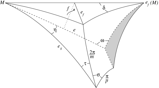
Figure 1. Polyhedron $\mathcal{P}^{*}$

Let $\mathcal{P}^{*}$ be the infinite volume polyhedron bounded by $\eta$, $\omega$, $\tau$, $\sigma$, and $\delta$. $\mathcal{P}^{*}$ has five right dihedral angles (between faces lying in $\eta$ and $\omega$, $\eta$ and $\tau$, $\delta$ and $\omega$, $\delta$ and $\tau$, and $\delta$ and $\sigma$). The plane $\sigma$ may either intersect with, or be parallel to, or be disjoint from each of $\tau$ and $\eta$.

If $\sigma$ and $\tau$ intersect, then we denote the dihedral angle of $\mathcal{P}^{*}$ between them by $2\pi/m$, where $m>2$, $m$ is not necessary an integer. We keep the notation $2\pi/m$ taking $m=\infty$ and $m=\overline{\infty}$ for parallel or disjoint $\sigma$ and $\tau$, respectively. Similarly, we denote the “dihedral angle” between $\eta$ and $\sigma$ by $\pi/p$, where $p>2$ is real, $\infty$, or $\overline{\infty}$. (We regard $\overline{\infty}>\infty>x$, $x/\infty=x/\overline{\infty}=0$, $\infty/x=\infty$, $\overline{\infty}/x=\overline{\infty}$ for any positive real $x$.) $\mathcal{P}^{*}$ exists in ${\mathbb{H}}^{3}$ for all $m>2$ and $p>2$ by [16].

In Figure 1, $\mathcal{P}^{*}$ is drawn under assumption that $m<\infty$, $p<\infty$, and $1/2+1/p+2/m>1$. The shaded triangle shows the hyperbolic plane orthogonal to $\eta$, $\sigma$, and $\omega$. Note that this plane is not a face of $\mathcal{P}^{*}$ and is shown only to underline the combinatorial structure of $\mathcal{P}^{*}$. In figures, we do not label dihedral angles of $\pi/2$ in order to not overload the picture.

Suppose now that $m<\infty$, that is $\sigma$ and $\tau$ intersect. Let $\xi$ be the plane passing through $e_{f}$ orthogonally to $\delta$. Then $\xi$ is orthogonal to $\omega$. One can see that $\sigma=R_{\xi}(\tau)$ and $\xi$ is the bisector of the dihedral angle of $\mathcal{P}^{*}$ made by $\tau$ and $\sigma$.

Let $\mathcal{Q}^{*}$ be the polyhedron bounded by $\eta$, $\tau$, $\omega$, $\delta$, and $\xi$. $\mathcal{Q}^{*}$ has six dihedral angles of $\pi/2$; the dihedral angle between $\tau$ and $\xi$ is equal to $\pi/m$ with $2<m<\infty$. Denote the “dihedral angle” between $\eta$ and $\xi$ by $\pi/k$, where $k>2$ is real, $k=\infty$, or $k=\overline{\infty}$. $\mathcal{Q}^{*}$ exists in ${\mathbb{H}}^{3}$ for all $m>2$ and $k>2$ by [16]. Note that $R_{\xi}$ is not necessary in $\Gamma^{*}$, but if it is and if $\Gamma^{*}$ is discrete, then we will see that $\mathcal{Q}^{*}$ is a fundamental polyhedron for $\Gamma^{*}$. In Figure 2, $\mathcal{Q}^{*}$ is drawn under assumption that $1/2+1/k+1/m>1$.

Figure 2. Polyhedron $\mathcal{Q}^{*}$

Lemma 2.2.

Let $f\in{\rm PSL}(2,{\mathbb{C}})$ be a $\pi$-loxodromic element, $g\in{\rm PSL}(2,{\mathbb{C}})$ be a parabolic element, and let $\Gamma=\langle f,g\rangle$ be a non-elementary $\mathcal{RP}$ group without invariant plane. Then there exist unique elements $h_{1},h_{2}\in{\rm PSL}(2,{\mathbb{C}})$ such that

• $h_{1}^{2}=fg^{-1}f^{-1}g^{-1}$ and $(h_{1}g)^{2}=1$,

• $h_{2}^{2}=f^{-1}g^{-1}f^{2}gf^{-1}$ and $(h_{2}fg^{-1}f^{-1})^{2}=1$.

Moreover, the elements $h_{1}$ and $h_{2}$ are not strictly loxodromic.

Proof.

First, note that $R_{\sigma}=e_{f}R_{\tau}e_{f}$ and $g=R_{\tau}R_{\omega}$. Therefore,

(2.2) $$R_{\sigma}R_{\omega}=e_{f}R_{\tau}e_{f}R_{\omega}=e_{f}R_{\tau}R_{\omega}e_{f}=e_{f}ge_{f}=fg^{-1}f^{-1}.$$

Let us show that if we take $h_{1}=R_{\xi}R_{\tau}=R_{\sigma}R_{\xi}$, then the assertion (1) of the lemma hold. Indeed,

$$h_{1}^{2}=R_{\sigma}R_{\tau}=(R_{\sigma}R_{\omega})(R_{\omega}R_{\tau})=fg^{-1}f^{-1}g^{-1}.$$

Moreover, $h_{1}g=(R_{\xi}R_{\tau})(R_{\tau}R_{\omega})=R_{\xi}R_{\omega}$. Since $\xi$ and $\omega$ are orthogonal, $(R_{\xi}R_{\omega})^{2}=1$. Hence, $(h_{1}g)^{2}=1$. Note also that since $h_{1}$ is a product of two reflections, $h_{1}$ is not strictly loxodromic.

Now let us show that $h_{1}$ is unique. The element $fg^{-1}f^{-1}g^{-1}$ is uniquely determined as an element of ${\rm PSL}(2,{\mathbb{C}})$.

If $fg^{-1}f^{-1}g^{-1}$ is parabolic, it has only one square root $h_{1}$. Suppose that $fg^{-1}f^{-1}g^{-1}$ is hyperbolic. Then it has exactly two square roots, one of which is $h_{1}$ defined above and the other, denoted $\overline{h}_{1}$, is a $\pi$-loxodromic element with the same axis and translation length as $h_{1}$. Clearly, $(\overline{h}_{1}g)^{2}\not=1$.

If $fg^{-1}f^{-1}g^{-1}$ is elliptic, then it also has two square roots $h_{1}$ and $\overline{h}_{1}$, both are elliptic elements. The element $\overline{h}_{1}$ is elliptic with the same axis as $h_{1}$ and with rotation angle $(\pi-2\pi/m)$, while $h_{1}$ is a rotation through $2\pi/m$ in the opposite direction. Again, $(\overline{h}_{1}g)^{2}\not=1$.

Now we take

$$h_{2}=R_{\eta}R_{\sigma}=(R_{\eta}R_{\tau})(R_{\tau}R_{\sigma})=e_{g}h_{1}^{-2}=efgf^{-1}.$$

Then

$$h_{2}^{2}=f^{-1}g^{-1}f^{2}gf^{-1}{\rm\quad and\quad}(fg^{-1}f^{-1}h_{2})^{2}=1.$$

These two conditions determine $h_{2}$ uniquely. ∎

Note that the elements $h_{1},h_{2}$ defined in Lemma 2.2 determine combinatorial and metric structures of $\mathcal{P}^{*}$. For example, if $h_{1}$ is elliptic, then its rotation angle is equal to the dihedral angle of $\mathcal{P}^{*}$ between $\sigma$ and $\tau$. If $h_{2}$ is elliptic, then its rotation angle is equal to the doubled dihedral angle of $\mathcal{P}^{*}$ between $\eta$ and $\sigma$. Vice versa, if the metric structure of $\mathcal{P}^{*}$ is fixed, then the types of elements $h_{1}$ and $h_{2}$ can be determined.

The same can be said about $\mathcal{Q}^{*}$ and the elements $h_{1}$ and $h_{2}h_{1}$. The element $h_{2}h_{1}$ is responsible for the mutual position of the planes $\eta$ and $\xi$ (see the proof of Lemma 2.5).

Lemmas 2.3–2.5 below give some necessary conditions for discreteness of $\Gamma$ via conditions on elements $h_{1}$ and $h_{2}$. One needs to keep in mind the connection between these elements and the polyhedra $\mathcal{P}^{*}$ and $\mathcal{Q}^{*}$.

Lemma 2.3.

If $\Gamma$ is discrete, then $h_{1}$ is either a hyperbolic, or parabolic, or primitive elliptic element of order $m\geq 3$.

Proof.

The subgroup $H=\langle g,fgf^{-1}\rangle$ of $\Gamma$ keeps $\delta$ invariant and is conjugate to a subgroup of ${\rm PSL}(2,\mathbb{R})$. Since $\Gamma$ is discrete, $H$ must be discrete. By [15] or [2], the group $H$ is discrete if and only if either

(1) $fg^{-1}f^{-1}g^{-1}=h_{1}^{2}$ is a hyperbolic, or a parabolic, or a primitive elliptic element, or

(2) $h_{1}$ is a primitive elliptic element of odd order $m$, where $m\geq 3$.

If $h_{1}^{2}$ is parabolic of hyperbolic, then $h_{1}$ is parabolic or hyperbolic, respectively. If $h_{1}^{2}$ is a primitive elliptic element, then $h_{1}$ is a primitive elliptic of even order $m\geq 4$. ∎

Lemma 2.4.

If $\Gamma$ is discrete, then $h_{2}$ is either a hyperbolic, or parabolic, or primitive elliptic element of order $p\geq 3$.

Proof.

Let $\kappa$ be the plane orthogonal to $\eta$, $\sigma$, and $\omega$. The subgroup $H=\langle e,fgf^{-1}\rangle$ of $\widetilde{\Gamma}$ keeps the plane $\kappa$ invariant and is conjugate to a subgroup of ${\rm PSL}(2,\mathbb{R})$. By [15], $H$ is discrete if and only if $h_{2}=efgf^{-1}$ is either a hyperbolic, or parabolic, or primitive elliptic element of order $p\geq 3$. ∎

Lemma 2.5.

If $\Gamma$ is discrete and $h_{1}$ is a primitive elliptic element of odd order, then $h_{2}h_{1}$ is either a hyperbolic, or parabolic, or primitive elliptic element of order $k\geq 3$.

Proof.

Recall that $\Gamma^{*}=\langle e_{f},R_{\eta},R_{\tau},R_{\omega}\rangle$. Since $h_{1}$ has odd order and $h_{1}^{2}\in\Gamma^{*}$, $h_{1}\in\Gamma^{*}$. Since, moreover, $h_{1}=R_{\xi}R_{\tau}$, $e_{f}=R_{\delta}R_{\xi}$, and $R_{\tau}\in\Gamma^{*}$, both $R_{\xi}$ and $R_{\delta}$ are also in $\Gamma^{*}$. Further, since the plane $\xi$ is orthogonal to $\omega$, the group $\langle R_{\eta}R_{\delta},e_{f}\rangle$ keeps $\omega$ invariant and is conjugate to a subgroup of ${\rm PSL}(2,\mathbb{R})$. It is clear that $\langle R_{\eta}R_{\delta},e_{f}\rangle$ is discrete if and only if $R_{\eta}R_{\xi}=h_{2}h_{1}$ is a hyperbolic, parabolic, or primitive elliptic element of order $k\geq 3$ [15]. ∎

Proof of Theorem 2.1. Lemma 2.2 proves existence and uniqueness of elements $h_{1}$ and $h_{2}$. Now we prove part (2) of the theorem.

If $\Gamma$ is discrete then $h_{1}$ is either a hyperbolic, or parabolic, or primitive elliptic element of order $m\geq 3$ by Lemma 2.3. We split the discrete groups $\Gamma$ into two families. The first family consists of those groups for which $h_{1}$ is hyperbolic, parabolic, or primitive elliptic of even order. By Lemma 2.4, for these groups $h_{2}$ is a hyperbolic, parabolic, or primitive elliptic element.

The second family consists of the discrete groups with $h_{1}$ elliptic of odd order. Then by Lemma 2.5, $h_{2}h_{1}$ is a hyperbolic, or parabolic, or primitive elliptic element of order $k\geq 3$. (Note that in this case $h_{2}$ is necessarily hyperbolic or primitive elliptic.)

So if $\Gamma$ is discrete, then either (2)(i) or (2)(ii) of Theorem 2.1 can occur. Clearly, if neither (2)(i) nor (2)(ii) holds, then $\Gamma$ is not discrete by Lemmas 2.3–2.5.

Now prove that each of (2)(i) and (2)(ii) is a sufficient condition for $\Gamma$ to be discrete. In each of the two cases we will give a fundamental polyhedron for $\Gamma^{*}$ to show, by using the Poincaré polyhedron theorem [3], that $\Gamma^{*}$ is discrete.

Suppose that (2)(i) holds. Then since $m$ is even, the group $G_{1}$ generated by the side pairing transformations $R_{\eta}$, $R_{\omega}$, $R_{\sigma}$, $R_{\tau}$, and $e_{f}$ and the polyhedron $\mathcal{P}^{*}$ satisfy the Poincaré polyhedron theorem, $G_{1}$ is discrete and $\mathcal{P}^{*}$ is its fundamental polyhedron. Obviously, $G_{1}=\Gamma^{*}$.

Suppose that (2)(ii) holds. Then the group $G_{2}$ generated by the side pairing transformations $R_{\eta}$, $R_{\omega}$, $R_{\xi}$, $R_{\tau}$, and $R_{\delta}$ and the polyhedron $\mathcal{Q}^{*}$ satisfy the Poincaré theorem, $G_{2}$ is discrete, and $\mathcal{Q}^{*}$ is its fundamental polyhedron.

In the proof of Lemma 2.5 it was shown that, for $m$ odd, $R_{\xi}\in\Gamma^{*}$ and $R_{\delta}\in\Gamma^{*}$. Moreover, $e_{f}=R_{\xi}R_{\delta}$. Hence, $G_{2}=\Gamma^{*}$, so $\Gamma^{*}$ is discrete.

Theorem 2.1 is proved.∎

Our next goal is to compute parameters $(\beta(f),\beta(g),\gamma(f,g))$ for both series of discrete groups listed in Theorem 2.1.

If $f\in{\rm PSL}(2,{\mathbb{C}})$ is a loxodromic element with translation length $d_{f}$ and rotation angle $\theta_{f}$, then

$${\rm tr}^{2}f=4\cosh^{2}\frac{d_{f}+i\theta_{f}}{2}$$

and $\lambda_{f}=d_{f}+i\theta_{f}$ is called the complex translation length of $f$.

Note that if $f$ is hyperbolic then $\theta_{f}=0$ and ${\rm tr}^{2}f=4\cosh^{2}(d_{f}/2)$. If $f$ is elliptic then $d_{f}=0$ and ${\rm tr}^{2}f=4\cos^{2}(\theta_{f}/2)$. If $f$ is parabolic then ${\rm tr}^{2}f=4$; by convention we set $d_{f}=\theta_{f}=0$.

We define the set

$$\mathcal{U}=\{u:u=i\pi/p{\rm\ for\ some\ }p\in{\mathbb{Z}},p\geq 2\}\cup[0,+\infty).$$

In other words, the set $\mathcal{U}$ consists of all complex translation half-lengths $u=\lambda_{f}/2$ for hyperbolic, parabolic, and primitive elliptic elements $f$. Furthermore, we define a function $t:\mathcal{U}\to\{2,3,4,\dots\}\cup\{\infty,\overline{\infty}\}$ as follows:

$$t(u)=\left\{\begin{array}[]{lll}p&{\rm if}&u=i\pi/p,\\ \infty&{\rm if}&u=0,\\ \overline{\infty}&{\rm if}&u\in(0,+\infty).\end{array}\right.$$

Given $u\in\mathcal{U}$ and $f$ with ${\rm tr}^{2}f=4\cosh^{2}u$, $t(u)$ determines the type of $f$ and, moreover, its order if $f$ is elliptic. Note also that since we regard $\infty/n=\infty$ and $\overline{\infty}/n=\overline{\infty}$, an expression of the form $(t(u),n)=1$ with $n>1$ means, in particular, that $t(u)$ is finite.

Theorem 2.6.

Let $f,g\in{\rm PSL}(2,{\mathbb{C}})$ with $\beta(f)<-4$, $\beta(g)=0$, and $\gamma(f,g)>0$. Then $\Gamma=\langle f,g\rangle$ is discrete if and only if one of the following holds:

1. $\gamma(f,g)=4\cosh^{2}u$ and $\beta(f)=-4\cosh^{2}v/\gamma(f,g)-4$, where $u,v\in\mathcal{U}$ with $t(u)\geq 4$, $(t(u),2)=2$, and $t(v)\geq 3$;

2. $\gamma(f,g)=4\cosh^{2}u$ and $\beta(f)=-4\cosh^{2}v-4$, where $u,v\in\mathcal{U}$ with $t(u)\geq 3$, $(t(u),2)=1$, and $t(v)\geq 3$.

Proof.

Obviously, $\beta(f)<-4$ and $\beta(g)=0$ if and only if $f$ is $\pi$-loxodromic and $g$ is parabolic. With this choice of $\beta(f)$ and $\beta(g)$, $\gamma(f,g)>0$ if and only if the group $\Gamma=\langle f,g\rangle$ is a non-elementary $\mathcal{RP}$ group without invariant plane [9]. This means that the hypotheses of Theorem 2.6 are equivalent to the hypotheses of Theorem 2.1. Therefore, in order to prove Theorem 2.6 it is sufficient to calculate the parameters $\beta(f)$ and $\gamma(f,g)$ for both families of the discrete groups listed in Theorem 2.1.

Let $\sigma^{\prime}$ be the image of $\sigma$ under $R_{\omega}$, that is $R_{\sigma^{\prime}}=R_{\omega}R_{\sigma}R_{\omega}$. Using the identity (2.2) and the fact that $g=R_{\tau}R_{\omega}$, we have

$$[f,g]=fgf^{-1}g^{-1}=(R_{\omega}R_{\sigma})(R_{\omega}R_{\tau})=(R_{\sigma^{\prime}}R_{\omega})(R_{\omega}R_{\tau})=R_{\sigma^{\prime}}R_{\tau}.$$

Note that $\sigma^{\prime}$ and $\tau$ are disjoint and $\delta$ is orthogonal to both of them. Therefore, $[f,g]$ is a hyperbolic element with the axis lying in $\delta$ and the translation length $2d$, where $d$ is the distance between $\sigma^{\prime}$ and $\tau$. Hence, since $\gamma(f,g)>0$,

$$\gamma(f,g)={\rm tr}[f,g]-2=+2\cosh d-2.$$

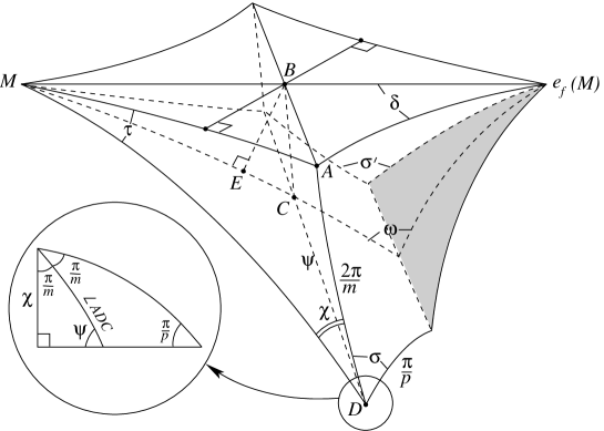
Figure 3.

Now, using generalised triangles in the plane $\delta$, it is not difficult to calculate that

$$\gamma(f,g)=\left\{\begin{array}[]{lll}4\cos^{2}(\pi/m)&{\rm if}&3\leq m<\infty,\\ 4&{\rm if}&m=\infty,\\ 4\cosh^{2}(d(\sigma,\tau)/2)&{\rm if}&m=\overline{\infty},\\ \end{array}\right.$$

where $d(\sigma,\tau)$ is the distance between $\sigma$ and $\tau$ if they are disjoint. Hence,

$$\gamma(f,g)=4\cosh^{2}u,$$

where $u\in\mathcal{U}$, $t(u)=m\geq 3$.

Let us calculate $\beta(f)$. The element $f$ is $\pi$-loxodromic if and only if ${\rm tr}^{2}f=4\cosh^{2}(T+i\pi/2)=-4\sinh^{2}T$, where $2T$ is the translation length of $f$. That is,

$$\beta(f)=-4\sinh^{2}T-4.$$

Note that $T$ is the distance between $e$ and $e_{f}$. It is measured in $\omega$ and equals $BE$ (see Figure 3).

Suppose that we are in case (2)(i) of Theorem 2.1, that is $(t(u),2)=2$, and that $\sigma$ and $\tau$ intersect. Recall that $\xi$ is the bisector of the dihedral angle of $\mathcal{P}^{*}$ made by $\sigma$ and $\tau$. Let $\psi$ be the angle that $\xi$ makes with $\eta$. Note that $\psi=\angle BCE$. From the link of $D$, we have that

$$\cos\chi=\frac{\cos(\pi/p)}{\sin(2\pi/m)}=\frac{\cos\psi}{\sin(\pi/m)}$$

and, therefore,

(2.3) $$\cos\psi=\frac{\cos(\pi/p)}{2\cos(\pi/m)}.$$

Further, from the link of $D$,

(2.4) $$\cos\angle ADC=\frac{\cos\psi\cdot\cos(\pi/m)}{\sin\psi\cdot\sin(\pi/m)}.$$

From the $\triangle ABM$, $\cosh^{2}AB=1/\sin(\pi/m)$ and, from the quadrilateral $ABCD$,

(2.5) $$\sinh BC=\frac{\cos\angle ADC}{\sinh AB}$$

Finally, from $\triangle BCE$,

(2.6) $$\sinh T=\sinh BE=\sin\psi\cdot\sinh BC.$$

Combining (2.3)–(2.6), we have that

$$\sinh^{2}T=\frac{\cos^{2}(\pi/p)}{4\cos^{2}(\pi/m)}=\frac{\cos^{2}(\pi/p)}{\gamma(f,g)}.$$

Similar calculations can be done for parallel or disjoint $\sigma$ and $\tau$. Hence, $\beta(f)=-\sinh^{2}T-4=-\cosh^{2}v/\gamma(f,g)-4$, where $v\in\mathcal{U}$, $t(v)\geq 3$.

Now note that in case (2)(ii) of Theorem 2.1, the angle $\psi=\angle BCE$ must be of the form $\pi/k$, $k\geq 3$ is an integer, $\infty$, or $\overline{\infty}$. Then we need to recompute the formulas (2.4)–(2.6) with $\psi=\pi/k$:

$$\cos\angle ADC=\frac{\cos(\pi/k)\cdot\cos(\pi/m)}{\sin(\pi/k)\cdot\sin(\pi/m)},\quad\sinh BC=\frac{\cos\phi}{\sinh a}=\frac{\cos(\pi/k)}{\sin(\pi/k)}.$$

Then

$$\sinh T=\sin\psi\cdot\sinh BC=\cos(\pi/k).$$

Hence, $\beta(f)=-4\cosh^{2}v-4$, where $v\in\mathcal{U}$, $t(v)\geq 3$. ∎

3. Orbifolds

Denote by $\Omega(\Gamma)$ the discontinuity set of a Kleinian group $\Gamma$. The Kleinian orbifold $Q(\Gamma)=({\mathbb{H}}^{3}\cup\Omega(\Gamma))/\Gamma$ is said to be an orientable $3$-orbifold with a complete hyperbolic structure on its interior ${\mathbb{H}}^{3}/\Gamma$ and a conformal structure on its boundary $\Omega(\Gamma)/\Gamma$.

We need the following (Kleinian) group presentations:

• $PH[\infty,m;q]=\langle x,y,s\,|\,x^{\infty}=s^{2}=(xs)^{2}=(ys)^{2}=(xyxy^{-1})^{m}=(y^{-1}xys)^{q}=1\rangle$,

• $P[\infty,m;q]=\langle w,x,y,z\,|\,w^{\infty}=x^{2}=y^{2}=z^{2}=(wx)^{2}=(wy)^{2}=(yz)^{2}=(zx)^{q}=(zw)^{m}=1\rangle$,

• $\mathcal{S}_{2}[\infty,m;q]=\langle x,L\,|\,x^{\infty}=(xLxL^{-1})^{m}=(xL^{2}x^{-1}L^{-2})^{q}=1\rangle$,

• $GTet_{1}[\infty,m;q]=\langle x,y,z\,|\,x^{\infty}=y^{2}=z^{\infty}=(xy)^{m}=(yzy^{-1}z^{-1})^{q}=[x,z]=1\rangle$.

Here $m$ and $q$ are integers greater than 1, or $\infty$ or $\overline{\infty}$ with the following convention. If we have a relation of the form $w^{n}=1$ with $n=\overline{\infty}$, then we simply remove the relation $w^{n}=1$ from the presentation (in fact, this means that the element $w$ is hyperbolic). Further, if $n=\infty$ and we keep the relation $w^{n}=1\sim w^{\infty}=1$, we get a Kleinian group presentation where parabolics are indicated. To get an abstract group presentation, we need to remove all relations of the form $w^{\infty}=1$.

Theorem 3.1.

Let $\Gamma=\langle f,g\rangle$ be a non-elementary discrete $\mathcal{RP}$ group without invariant plane. Let $\beta(f)\in(-\infty,-4)$ and let $\beta(g)=0$. Then $\gamma(f,g)=4\cosh^{2}u$, where $u\in\mathcal{U}$, $t(u)\geq 3$, and one of the following holds:

1. If $(t(u),2)=2$ and $\beta(f)=-4\cosh^{2}v/\gamma(f,g)-4$, where $v\in\mathcal{U}$, $t(v)\geq 3$, $(t(v),2)=1$, then $\Gamma$ is isomorphic to $PH[\infty,t(u)/2;t(v)]$.

2. If $(t(u),2)=2$ and $\beta(f)=-4\cosh^{2}v/\gamma(f,g)-4$, where $v\in\mathcal{U}$, $t(v)\geq 4$, $(t(v),2)=2$, then $\Gamma$ is isomorphic to $\mathcal{S}_{2}[\infty,t(u)/2;t(v)/2]$.

3. If $(t(u),2)=1$ and $\beta(f)=-4\cosh^{2}v-4$, where $v\in\mathcal{U}$, $t(v)\geq 3$, $(t(v),2)=1$, then $\Gamma$ is isomorphic to $P[\infty,t(u);t(v)]$.

4. If $(t(u),2)=1$ and $\beta(f)=-4\cosh^{2}v-4$, where $v\in\mathcal{U}$, $t(v)\geq 4$, $(t(v),2)=2$, then $\Gamma$ is isomorphic to $GTet_{1}[\infty,t(u);t(v)/2]$.

Proof.

Suppose $(t(u),2)=2$, that is the dihedral angle of $\mathcal{P}^{*}$ between $\sigma$ and $\tau$ is $2\pi/m$ with $m$ even, $\infty$, or $\overline{\infty}$. Consider a polyhedron $\widetilde{\mathcal{P}}$ bounded by $\sigma$, $\tau$, $\sigma^{\prime}=R_{\omega}(\sigma)$, $\tau^{\prime}=R_{\omega}(\tau)$, $\eta$, and $\delta$. Applying the Poincaré theorem to $\widetilde{\mathcal{P}}$ and the side pairing transformations $g$, $g^{\prime}=R_{\sigma}R_{\omega}$, $e$, and $e_{f}$, one can see that $\langle g,g^{\prime},e_{f},e\rangle$ is isomorphic to $\widetilde{\Gamma}$ and has the presentation

$$\langle f,g,e\,|\,g^{\infty}=e^{2}=(ef)^{2}=(eg)^{2}=(gfgf^{-1})^{m/2}=(f^{-1}gfe)^{p}=1\rangle.$$

If $p$ is odd, then $e\in\langle f,g\rangle$ and $\widetilde{\Gamma}=\Gamma\cong PH[\infty,m/2;p]$.

If $p$ is even, $\infty$, or $\overline{\infty}$, then $\widetilde{\Gamma}$ contains $\Gamma$ as a subgroup of index $2$ and has presentation $\mathcal{S}_{2}[\infty,m/2;p/2]$. In order to see this, one can apply the Poincaré theorem to a polyhedron $\mathcal{P}$ bounded by $\tau$, $\sigma$, $\tau^{\prime}$, $\sigma^{\prime}$, $\eta$, and $e_{f}(\eta)$, and side-pairing transformations $f$, $g$, and $g^{\prime}=fg^{-1}f^{-1}$.

The proof for $(t(u),2)=1$ is analogous. In this case we need to use the polyhedron $\mathcal{Q}^{*}$ as the starting point. ∎

(a) $\pi_{1}^{orb}(Q)\cong PH[\infty,m;q]$	(b) $\pi_{1}(Q)^{orb}\cong P[\infty,m;q]$
$m\geq 2$, $q\geq 3$	$m\geq 3$, $q\geq 3$

Figure 4. Orbifolds embedded in ${\mathbb{S}}^{3}$

(a) $\pi_{1}^{orb}(Q)\cong\mathcal{S}_{2}[\infty,m;q]$	(b) $\pi_{1}^{orb}(Q)\cong GTet_{1}[\infty,m;q]$
$m\geq 2$, $q\geq 2$	$m\geq 3$, $q\geq 2$

Figure 5. Orbifolds embedded in Seifert fibred spaces

The orbifolds $Q(\Gamma)$ for the groups described in Theorem 3.1 can be obtained from corresponding fundamental polyhedra. In Figures 4 and 5, we schematically draw singular sets, cusps, and boundary components of $Q(\Gamma)$ by using fat vertices and fat edges. Roughly speaking, a fat vertex is either an interior point, or is removed, or removed together with its regular neighbourhood depending on the indices. A fat edge can be labelled by $\infty$ or $\overline{\infty}$. If the index at a fat edge is $\infty$, then the egde corresponds to a cusp, and if the index is $\overline{\infty}$, the edge is removed together with its regular neighbourhood. For details, see [12].

In Figure 4, orbifolds are embedded in ${\mathbb{S}}^{3}$ so that $\infty$ is a non-singular interior point of $Q(\Gamma)$. Note that the volume of $Q(PH[\infty,m;q])$ is always infinite and $Q(P[\infty,m;q])$ is always non-compact.

Let $T(n)$ be a Seifert fibred solid torus obtained from a trivial fibred solid torus $D^{2}\times{\mathbb{S}}^{1}$ by cutting it along $D^{2}\times\{x\}$ for some $x\in{\mathbb{S}}^{1}$, rotating one of the discs through $2\pi/n$ and glueing back together.

Denote by $\mathcal{S}(n)$ a space obtained by glueing two copies of $T(n)$ along their boundaries fibre to fibre. Clearly, $\mathcal{S}(n)$ is homeomorphic to ${\mathbb{S}}^{2}\times{\mathbb{S}}^{1}$ and is $n$-fold covered by trivially fibred ${\mathbb{S}}^{2}\times{\mathbb{S}}^{1}$. There are two critical fibres whose length is $n$ times shorter than the length of a regular fibre.

In Figure 5(a), orbifolds are embedded in Seifert fibre spaces $\mathcal{S}(2)=T(2)\cup T(2)$. We draw only the solid torus that contains singular points (or boundary components). The other fibred torus is meant to be attached and is not shown. If $m<\infty$, the orbifold $Q(\mathcal{S}_{2}[\infty,m;q])$ is embedded in $\mathcal{S}(2)$ in such a manner that the axis of order $m$ lies on a critical fibre of $\mathcal{S}(2)$. The removed regular fibre gives rise to a cusp.

In Figure 5(b), orbifolds are embedded in trivially fibred space ${\mathbb{S}}^{2}\times{\mathbb{S}}^{1}$. The rank 2 cusp corresponds to the subgroup of $GTet_{1}[\infty,m;q]$ generated by $x$ and $z$.

4. Structure of the slice $S_{\infty}$

Recall that

$$S_{\infty}=\{(\gamma,\beta):(\beta,0,\gamma){\rm\ are\ parameters\ for\ some\ }\langle f,g\rangle\in\mathcal{DRP}\},$$

where $\mathcal{DRP}$ denotes the class of all non-elementary discrete $\mathcal{RP}$ groups.

To investigate the slice $S_{\infty}$, we split the plane $(\gamma,\beta)$ as follows.

• If $\beta=-4$ then by [9, Theorem 2], the group $\langle f,g\rangle$ has an invariant plane. We use [5] to find all discrete groups on the line $\beta=-4$.

• If $\beta>-4$ and $\gamma>0$ then the group $\langle f,g\rangle$ is conjugate to a subgroup of ${\rm PSL}(2,{\mathbb{R}})$. More precisely, if $-4<\beta<0$ then $f$ is elliptic and the axis of $f$ is orthogonal to an invariant plane of $g$ and if $\beta=0$ then the fixed points of $f$ and $g$ lie in their common invariant plane. Discreteness criteria in terms of traces of $f$, $g$, and $fg$ were given in [14]. For $\beta>0$, an algorithm to decide whether $f$ and $g$ generate a discrete group was given in [8].

• If $\beta>-4$ and $\gamma<0$ then $f$ is elliptic, parabolic, or hyperbolic and the group $\langle f,g\rangle$ is known to be truly spatial. Discrete such groups are described in [11], where $\beta$ and $\gamma$ are found explicitly.

• If $\beta<-4$ and $\gamma<0$ then $f$ is $\pi$-loxodromic whose axes lies in an invariant plane of $g$. Then this plane is invariant under action of $\langle f,g\rangle$ and $f$ acts as a glide-reflection on it. A geometrical description of such discrete groups was given in [13].

• The case of $\beta<-4$ and $\gamma>0$ was treated in Section 2 of the present paper.

We will obtain explicit formulas for $\beta$ and $\gamma$ in the cases 2 and 4 above and completely describe the structure of the slice $S_{\infty}$. We will pay special attention to the subsets of $S_{\infty}$ corresponding to free groups.

First, we need the following elementary facts.

Lemma 4.1.

If $f,g\in{\rm PSL}(2,{\mathbb{C}})$ and $g$ is parabolic, then

$$\gamma(f,g)=({\rm tr}(fg)-{\rm sign}({\rm tr}g)\cdot{\rm tr}f)^{2}.$$

Proof.

By the Fricke identity, we have

$$\gamma(f,g) = {\rm tr}[f,g]-2$$

$$= {\rm tr}^{2}f+{\rm tr}^{2}g+{\rm tr}^{2}(fg)-{\rm tr}f\cdot{\rm tr}g\cdot{\rm tr}(fg)-4$$

$$= ({\rm tr}(fg)-{\rm sign}({\rm tr}g)\cdot{\rm tr}f)^{2},$$

since ${\rm tr}^{2}g=4$. ∎

Lemma 4.2.

If $f,g\in{\rm PSL}(2,{\mathbb{C}})$ and ${\rm tr}g=2$, then

$${\rm tr}(fg^{k})=k({\rm tr}(fg)-{\rm tr}f)+{\rm tr}f.$$

Proof.

By substituting ${\rm tr}g=2$ into the recurrent formula

$${\rm tr}(fg^{k})={\rm tr}(fg^{k-1}){\rm tr}g-{\rm tr}(fg^{k-2}),$$

we immediately get the result. ∎

Remark 4.3.

Suppose that $f$ is non-primitive elliptic of finite order $n$, i.e., $\beta(f)=-4\sin^{2}(q\pi/n)$, where $(q,n)=1$, $1<q<n/2$. Then there exists an integer $r$ so that $f^{r}$ is primitive of the same order. Obviously, $\langle f,g\rangle=\langle f^{r},g\rangle$ and $\beta(f^{r})=-4\sin^{2}(\pi/n)$. By [7], $\gamma(f^{r},g)=(\beta(f^{r})/\beta(f))\gamma(f,g)$.

It is natural to introduce the constant

$$C(q,n)=\frac{\sin^{2}(q\pi/n)}{\sin^{2}(\pi/n)}=\frac{\beta(f)}{\beta(f^{r})}\geq 1$$

that plays an important role in parameters calculation concerning groups with elliptic elements. It is also convenient to consider a parabolic element $f$ as a limit rotation of order $n=\infty$ and write $0=\beta(f)=-4\sin^{2}(\pi/n)$ with $C(q,n)=C(1,n)=1$.

4.1. $-4\leq\beta\leq 0$

This means that $f$ is either elliptic or parabolic. Obviously, if $f$ is elliptic of infinite order, then $\langle f,g\rangle$ is not discrete. So we assume that $\beta=-4\sin^{2}(q\pi/n)$, where $(q,n)=1$ and $1\leq q<n/2$, including $\beta=0$.

Theorem 4.4.

Let $\Gamma=\langle f,g\rangle\subset{\rm PSL}(2,{\mathbb{C}})$ have parameters $(\beta,0,\gamma)$ with $\gamma\in{\mathbb{R}}\backslash\{0\}$. Let $\beta=-4\sin^{2}(q\pi/n)$, where $(q,n)=1$ and $1\leq q<n/2$, including $\beta=0$. Then $\Gamma$ is discrete if and only if one of the following holds:

1. $\gamma=-4C(q,n)\cosh^{2}u$, where $u\in\mathcal{U}$ and $t(u)\geq 3$;

2. $\gamma=4C(q,n)(\cos(\pi/n)+\cosh u)^{2}$, where $u\in\mathcal{U}$;

3. $\beta=0$ and $\gamma=4(1+\cos(2\pi/k))^{2}$, where $k\geq 3$ is odd.

Proof.

Let us prove the theorem for $q=1$; in order to get the result for $q>1$, we only need to apply Remark 4.3.

If $n=2$ then $\beta=-4$ and, by [5, Theorem 4.15], $\Gamma$ is discrete if and only if $\gamma=\pm 4\cosh^{2}u$, where $u\in\mathcal{U}$ with $t(u)\geq 3$.

If $2<n\leq\infty$ and $\gamma<0$, then, by [11, Corollary 2.5], $\Gamma$ is discrete if and only if $\gamma=-4\cosh^{2}u$, where $u\in\mathcal{U}$ and $t(u)\geq 3$.

Assume that $2<n<\infty$ and $\gamma>0$. In this case $\Gamma$ is conjugate to a subgroup of ${\rm PSL}(2,{\mathbb{R}})$ and we can apply Knapp’s results [14] to compute $\gamma$. Conjugate $\Gamma$ so that $\infty$ is the fixed point of $g$. By replacing, if necessary, $f$ with $f^{-1}$ and $g$ with $g^{-1}$, we may assume that

$$f=\left(\begin{array}[]{cc}a&b\\ c&d\end{array}\right)\quad{\rm and}\quad g=\left(\begin{array}[]{rr}-1&\tau\\ 0&-1\end{array}\right),$$

where $ad-bc=1$, $a+d=-2\cos(\pi/n)$ with $n\in{\mathbb{Z}}$, $b>0$, and $\tau>0$.

One can show that ${\rm tr}(fg)<2$. By [14, Proposition 4.1], $\Gamma$ is discrete if and only if ${\rm tr}(fg)\leq-2$ or ${\rm tr}(fg)=-2\cos(\pi/k)$, where $k\geq 2$ is an integer, that is ${\rm tr}(fg)=-2\cosh u$, where $u\in\mathcal{U}$. Hence, by Lemma 4.1, $\gamma=({\rm tr}(fg)+{\rm tr}f)^{2}=(2\cosh u+2\cos(\pi/n))^{2}$.

So it remains to consider the case when $n=\infty$ (i.e., $\beta=0$) and $\gamma>0$. Again, we normalize $\Gamma$ so that $g$ is as above and $f=\left(\begin{array}[]{rr}-1&0\\ -1&-1\end{array}\right)$. By [14, Proposition 4.2], such a group is discrete if and only if $\tau\geq 4$ or $\tau=2+2\cos(2\pi/k)$ for an integer $k\geq 3$. Since in this case $\gamma=\tau^{2}$, we have that $\gamma\geq 16$ or $\gamma=(2+2\cos(2\pi/k))^{2}$, which can be written as $\gamma=4(1+\cosh u)^{2}$, where $u\in\mathcal{U}$, or $\gamma=4(1+\cos(2\pi/k))^{2}$ for odd $k\geq 3$. ∎

Remark 4.5.

If $-4\leq\beta\leq 0$ then $\Gamma$ is discrete and free if and only if $\beta=0$ and $\gamma\in(-\infty,-4]\cup[16,+\infty)$.

The parameters from the infinite strip $-4\leq\beta\leq 0$ are displayed in Figure 6. If $\beta=-4\sin^{2}(q\pi/n)$ is fixed, then there exist values $\gamma_{1}(\beta)<0$ and $\gamma_{2}(\beta)>0$ so that $\Gamma$ is discrete in the union of two rays $(-\infty,\gamma_{1}(\beta)]\cup[\gamma_{2}(\beta),+\infty)$. There are only countably many discrete groups in $(\gamma_{1}(\beta),\gamma_{2}(\beta))$ with accumulation points $\gamma_{1}(\beta)$ and $\gamma_{2}(\beta)$.

Moreover, if we denote $\beta_{n}^{q}=-4\sin^{2}(q\pi/n)$, then

$$\gamma_{1}(\beta_{n}^{q})<\gamma_{1}(\beta_{n}^{1})<\gamma_{2}(\beta_{n}^{1})<\gamma_{2}(\beta_{n}^{q})\quad{\rm for\ all\ }1<q<n/2.$$

$\beta=-4\sin^{2}(\pi/n)$ with $n\in{\mathbb{Z}}$


$\beta=-4\sin^{2}(q\pi/n)$ with $(q,n)=1$ and $1\leq q<n/2$

Figure 6. Structure of the strip $-4\leq\beta\leq 0$

4.2. $\beta>0$

In this case $f$ is hyperbolic.

Theorem 4.6 ([11, Corollary 2.5]).

Let $\Gamma=\langle f,g\rangle\subset{\rm PSL}(2,{\mathbb{C}})$ have parameters $(\beta,0,\gamma)$ with $\beta>0$ and $\gamma<0$. Then $\Gamma$ is discrete if and only if $\gamma=-4\cosh^{2}u$, where $u\in\mathcal{U}$, $t(u)\geq 3$.

Remark 4.7.

From [11], $\Gamma$ with parameters $(\beta,0,\gamma)$, where $\beta\geq 0$ and $\gamma<0$ is free if and only if $(\gamma,\beta)$ lies in the region

$$A=\{(\gamma,\beta):\gamma\leq-4,\beta\geq 0\}.$$

Theorem 4.8.

Let $\Gamma=\langle f,g\rangle\subset{\rm PSL}(2,{\mathbb{C}})$ have parameters $(\beta,0,\gamma)$ with $\beta>0$ and $\gamma>0$. Let $k=\displaystyle\left\lceil\frac{\sqrt{\beta+4}-2}{\sqrt{\gamma}}\right\rceil$. The group $\Gamma$ is discrete if and only if one of the following holds:

1. $\beta=(k\sqrt{\gamma}+2)^{2}-4$ and $\gamma=16\cosh^{4}u$, where $u\in\mathcal{U}$ and $t(u)\geq 3$;

2. $\beta=(k\sqrt{\gamma}\pm 2\cos(q\pi/n))^{2}-4$ and $\gamma=4C(q,n)(\cos(\pi/n)+\cosh u)^{2}$, where $(q,n)=1$, $1\leq q<n/2$, and $u\in\mathcal{U}$;

3. $\beta=(k\sqrt{\gamma}-2\cosh u)^{2}-4$ and $\gamma>4(1+\cosh u)^{2}$, where $u\geq 0$.

Proof.

Since $\gamma>0$, the axis of $f$ lies in an invariant plane of $g$, so $\Gamma=\langle f,g\rangle$ is conjugate to a subgroup of ${\rm PSL}(2,{\mathbb{R}})$. In [8], an algorithm for determining whether such a group is discrete was given. We will apply this algorithm and calculate parameters for each discrete group.

Normalize $\Gamma$ so that $\infty$ is the fixed point of $g$ and $\pm 1$ are the fixed points of $f$. Then we can write

$$f=\left(\begin{array}[]{cc}a&b\\ b&a\end{array}\right)\quad{\rm and}\quad g=\left(\begin{array}[]{cc}1&\tau\\ 0&1\end{array}\right),\ {\rm where}\ a^{2}-b^{2}=1,\ a>1,\ b,\tau\in{\mathbb{R}}.$$

By replacing $f$ with $f^{-1}$ and $g$ with $g^{-1}$, we may assume that $b<0$ and $\tau>0$.

Let $k$ be a positive integer such that ${\rm tr}(fg^{k})\leq 2$ and ${\rm tr}(fg^{\ell})>2$ for all $\ell$ with $0\leq\ell<k$.

By Lemmas 4.1 and 4.2, we have that $k^{2}\gamma=k^{2}({\rm tr}(fg)-{\rm tr}f)^{2}=({\rm tr}(fg^{k})-{\rm tr}f)^{2}$. Since ${\rm tr}(fg^{k})\leq 2$ and ${\rm tr}f>2$,

(4.7) $${\rm tr}f=k\sqrt{\gamma}+{\rm tr}(fg^{k}).$$

We distinguish three cases:

1. ${\rm tr}(fg^{k})=2$, that is $fg^{k}$ is parabolic. From (4.7),

$$\beta=(k\sqrt{\gamma}+2)^{2}-4.$$

By Theorem 4.4, $\langle fg^{k},g\rangle$ and, hence, $\langle f,g\rangle$ is discrete if and only if

• $\gamma=\gamma(fg^{k},g)=4(1+\cosh v)^{2}$, where $v\in\mathcal{U}$, or

• $\gamma=4(1+\cos(2\pi/k))^{2}$, where $k\geq 3$ is odd.

These expressions can be rearranged and combined as $\gamma=16\cosh^{4}u$, where $u\in\mathcal{U}$ and $t(u)\geq 3$.

2. $-2<{\rm tr}(fg^{k})<2$, that is $fg^{k}$ is elliptic and ${\rm tr}(fg^{k})=\pm 2\cos(q\pi/n)$, where $(q,n)=1$ and $1\leq q<n/2$. Hence, from (4.7),

$$\beta=(k\sqrt{\gamma}\pm 2\cos(q\pi/n))^{2}-4.$$

By Theorem 4.4, $\langle fg^{k},g\rangle$ and, hence, $\langle f,g\rangle$ is discrete if and only if

$$\gamma=4C(q,n)(\cos(\pi/n)+\cosh u)^{2},\text{\quad where }u\in\mathcal{U}.$$

3. ${\rm tr}(fg^{k})\leq-2$, that is $fg^{k}$ is hyperbolic or parabolic so we can write ${\rm tr}(fg^{k})=-2\cosh u$, where $u\geq 0$. Then

$$\beta=(k\sqrt{\gamma}-2\cosh u)^{2}-4.$$

Consider the group $\langle g^{k-1}f,g\rangle$. The element $g^{k-1}f$ is hyperbolic with ${\rm tr}(g^{k-1}f)>2$. Therefore, one can normalize $\langle g^{k-1}f,g\rangle$ so that the attracting and repelling fixed points of $g^{k-1}f$ are $x_{a}$ and $x_{r}$, respectively, and $x_{a}<x_{r}$. Since ${\rm tr}(g^{k}f)\leq-2$, such a group is dicrete and free by [8, Case II]. So by Lemma 4.1, we have that

$$\gamma=\gamma(fg^{k-1},g) = ({\rm tr}(fg^{k})-{\rm tr}(fg^{k-1}))^{2}$$

$$= (2\cosh u+2\cosh v)^{2},$$

where $v$ is any positive real number.

It remains to compute $k$. Since ${\rm tr}(fg^{k})=2a+b\tau k\leq 2$, we have that $k\geq(-2a+2)/(b\tau)$. Computing $\gamma=b^{2}\tau^{2}$, we get $b\tau=-\sqrt{\gamma}$. So $k=\left\lceil\displaystyle\frac{\sqrt{\beta+4}-2}{\sqrt{\gamma}}\right\rceil$. ∎

It follows from [8] that $\Gamma$ is free if and only if $(\gamma,\beta)$ lies in one of the regions

$$C_{k}=\{(\gamma,\beta):\gamma\geq 16,((k-1)\sqrt{\gamma}+2)^{2}\leq\beta+4\leq(k\sqrt{\gamma}-2)^{2}\},\ k=1,2,3\dots$$

4.3. $\beta<-4$

First, consider $\gamma<0$. In this case the axis of the $\pi$-loxodromic generator $f$ lies in an invariant plane of $g$ [9], so $\langle f,g\rangle$ keeps this plane invariant.

Theorem 4.9.

Let $\Gamma=\langle f,g\rangle\subset{\rm PSL}(2,{\mathbb{C}})$ have parameters $(\beta,0,\gamma)$ with $\beta<-4$ and $\gamma<0$. Let $k=\displaystyle\left\lceil\frac{\sqrt{-\beta-4}}{\sqrt{-\gamma}}\right\rceil$. Then the group $\langle f,g\rangle$ is discrete if and only if one of the following holds:

1. $-4(\beta+4)=\big{(}(2k-1)\sqrt{-\gamma}\pm\sqrt{-\gamma-8(1+\cosh u)}\big{)}^{2}$, where $u\in\mathcal{U}$;

2. $4(\beta+4)=(2k-1)^{2}\gamma$ and $\gamma=-16\cos^{2}(\pi/p)$, where $p\geq 3$ is odd;

3. $\beta=k^{2}\gamma-4$ and $\gamma=-4\cosh^{2}u$, where $u\in\mathcal{U}$ and $t(u)\geq 3$.

Proof.

Let $\delta=\{(z,t):{\rm Im}\ z=0\}$ be the invariant plane of $\Gamma$. Since the axis of $f$ lies in $\delta$, we can normalize $\Gamma$ so that the fixed point of $g$ is $\infty$, the fixed points of $f$ are $\pm 1$, and

$$f=\left(\begin{array}[]{cc}ai&bi\\ bi&ai\end{array}\right),\quad g=\left(\begin{array}[]{cc}1&\tau\\ 0&1\end{array}\right),\quad{\rm where}\ b^{2}-a^{2}=1,\ a>1,\ b,\tau\in{\mathbb{R}}.$$

Further, replacing $f$ with $f^{-1}$ and $g$ with $g^{-1}$, we can assume that $b<0$ and $\tau>0$. Since $b$ is negative, $+1$ is the repelling fixed point of $f$ and $-1$ is attracting.

Let $e$ be the half-turn whose axis passes through the fixed point of $g$ orthogonally to the axis of $f$. That is $e$ fixes $0$ and $\infty$. Let $e_{f}$ and $e_{1}$ be half-turns such that $f=ee_{f}$ and $g=e_{1}e$. Since $f$ is $\pi$-loxodromic, the axis of $e_{f}$ intersects the axis of $f$ (and the plane $\delta$) orthogonally; denote the intersection point by $A$. Further, since $g$ is parabolic and keeps $\delta$ invariant, the axis of $e_{1}$ fixes $\infty$ and lies in the plane $\delta$. It is easy to calculate that

$$e=\left(\begin{array}[]{rr}i&0\\ 0&-i\end{array}\right),\quad e_{f}=\left(\begin{array}[]{rr}a&b\\ -b&-a\end{array}\right),\quad e_{1}=\left(\begin{array}[]{rr}i&\tau\\ 0&-i\end{array}\right).$$

Consider half-turns $e_{k-1}=g^{k-1}e$ and $e_{k}=g^{k}e$ such that $A$ lies in the region bounded by the axes of $e_{k-1}$ and $e_{k}$ in the plane $\delta$, see Figure 7. It is easy to calculate that $A=-a/b-j/b$. Since $e_{k}$ fixes $\infty$ and $\tau k/2$, we have that

$$A\in\left\{(z,t):\frac{\tau(k-1)}{2}<{\rm Re}z\leq\frac{\tau k}{2},\ {\rm Im}\ z=0,\ t>0\right\}.$$

Hence, we can immediately determine $k$.

(4.8) $$\frac{\tau(k-1)}{2}<-\frac{a}{b}\leq\frac{\tau k}{2}.$$

Therefore, since $2a=-i{\rm tr}f=\sqrt{-\beta-4}$ and $b\tau=-\sqrt{-\gamma}$,

$$k=\left\lceil-\frac{2a}{b\tau}\right\rceil=\left\lceil\frac{\sqrt{-\beta-4}}{\sqrt{-\gamma}}\right\rceil.$$

It is easy to see that $\Gamma$ is discrete if and only if $\widetilde{\Gamma}=\langle e_{f},e_{k-1},e_{k}\rangle$ is. Following [13], we give geometric conditions for $\widetilde{\Gamma}$ to be discrete.

Suppose that $A\notin axis(e_{k})$; see Figure 7(a). By [13], $\widetilde{\Gamma}$ is discrete if either

(a) the angle $\phi$ between $e_{k-1}$ and $e_{f}(e_{k})$ is of the form $\pi/p$, where $p\geq 2$ is an integer, $\infty$, or $\overline{\infty}$; or

(b) $\phi=2\pi/p$, where $p\geq 3$ is odd and the bisector of $\phi$ passes through $A$.

Suppose that $A\in axis(e_{k})$; see Figure 7(b). By [13], $\widetilde{\Gamma}$ is discrete if

(c) the angle $\psi$ made by $axis(e_{k-1})$ and $axis(\tilde{e}_{f})$ is of the form $\pi/p$, $p\geq 3$ is an integer, $\infty$, or $\overline{\infty}$, where $\tilde{e}_{f}=e_{k}e_{f}$ is the half-turn whose axis passes through $A$ orthogonally to $axis(e_{k})$ in the plane $\delta$.

(a)	(b)

Figure 7. The invariant plane $\delta$

There are no other discrete groups. So, we need to calculate the parameters $\beta$ and $\gamma$ in each of the cases (a), (b), and (c).

Assume that we are in case (a) or (b). Then each $g^{\ell}f=e_{\ell}e_{f}$, $\ell\in{\mathbb{Z}}$, is a $\pi$-loxodromic element with translation length $2T_{\ell}$ and ${\rm tr}(g^{\ell}f)=\pm 2i\sinh T_{\ell}$, where $T_{\ell}$ is the distance between $e_{\ell}$ and $A$. Moreover, from the matrix representation, ${\rm tr}(g^{\ell}f)=2ai+b\tau\ell i$. The inequalities (4.8) enable us to determine the signs of ${\rm tr}(fg^{k-1})$ and ${\rm tr}(fg^{k})$:

$${\rm tr}(fg^{k})=-2i\sinh T_{k}\quad{\rm and}\quad{\rm tr}(fg^{k-1})=+2i\sinh T_{k-1}.$$

Suppose that $p<\infty$. Simple calculations in the plane $\delta$ show that

$$\sinh CD=\frac{1+\cos\phi\cosh(2T_{k-1})}{\sin\phi\sinh(2T_{k-1})}$$

and, on the other hand,

$$\sinh CD=\frac{\sinh T_{k}+\cos\phi\sinh T_{k-1}}{\sin\phi\cosh T_{k-1}}.$$

So, we obtain

$$2(1+\cos\phi)=4\sinh T_{k-1}\sinh T_{k}={\rm tr}(fg^{k-1}){\rm tr}(fg^{k}).$$

Applying Lemmas 4.1 and 4.2 and the facts that ${\rm tr}f=i\sqrt{-\beta-4}$ and ${\rm tr}(fg)-{\rm tr}f=b\tau i=-i\sqrt{-\gamma}$, we get

$$2(1+\cos\phi) = [(k-1)({\rm tr}(fg)-{\rm tr}f)+{\rm tr}f]\cdot[k({\rm tr}(fg)-{\rm tr}f)+{\rm tr}f]$$

$$= k(k-1)({\rm tr}(fg)-{\rm tr}f)^{2}+(2k-1)\cdot{\rm tr}f\cdot({\rm tr}(fg)-{\rm tr}f)+{\rm tr}^{2}f$$

$$= k(k-1)\gamma+(2k-1)\sqrt{-\beta-4}\sqrt{-\gamma}+\beta+4.$$

Hence, $-4(\beta+4)=((2k-1)\sqrt{-\gamma}\pm\sqrt{-8(1+\cos\phi)-\gamma})^{2}$, where $\phi=\pi/p$, $p\geq 2$ is an integer. Analogous calculation can be done for $p=\infty$ and $p=\overline{\infty}$, and we obtain item (1) of the theorem.

In case (b), in addition, $T_{k-1}=T_{k}$. Then ${\rm tr}(fg^{k})=-{\rm tr}(fg^{k-1})$ and by Lemmas 4.1 and 4.2 we have

$$2\sqrt{-\beta-4}=(2k-1)\sqrt{-\gamma}.$$

Therefore, $2(1+\cos\phi)=-{\rm tr}^{2}(fg^{k})=(-k\sqrt{-\gamma}+\sqrt{-\beta-4})^{2}=-\gamma/4$. Hence, since $\phi=2\pi/p$, $\gamma=-16\cos^{2}(\pi/p)$.

Now assume that we are in case (c) and $p<\infty$. Since in this case $e_{k}e_{f}=\tilde{e}_{f}$ is an ellitic element of order $2$, ${\rm tr}(g^{k}f)=0$. Therefore, since ${\rm tr}(g^{k}f)=-ki\sqrt{-\gamma}+i\sqrt{-\beta-4}$, we have that $\beta=k^{2}\gamma-4$.

Further, since ${\rm tr}(fg^{k-1})=2i\sinh T_{k-1}$ and, from the plane $\delta$, $\sinh T_{k-1}=\cos\psi$, we have that

$$4\cos^{2}\psi=4\sinh^{2}T_{k-1} = -((k-1)({\rm tr}(fg)-{\rm tr}f)+{\rm tr}f)^{2}$$

$$= (-(k-1)\sqrt{-\gamma}+\sqrt{-\beta-4})^{2}$$

$$= (-(k-1)\sqrt{-\gamma}+k\sqrt{-\gamma})^{2}$$

$$= -\gamma.$$

Thus, $\gamma=-4\cos^{2}(\pi/p)$, where $p\geq 3$ is an integer. Analogous calculations can be done for $p=\infty$ and $p=\overline{\infty}$ and we obtain item (3) of the theorem. ∎

Remark 4.10.

If $\beta<-4$ and $\gamma<0$, then $\langle f,g\rangle$ is free if and only if $(\gamma,\beta)$ lies in one of the regions $D_{k}$, $k=1,2,3,\dots$, given by

$$D_{k}=\{ (\gamma,\beta):\gamma\leq-16,$$

$$\frac{((2k-1)\sqrt{-\gamma}-\sqrt{-\gamma-16})^{2}}{-4}\geq\beta+4\geq\frac{((2k-1)\sqrt{-\gamma}+\sqrt{-\gamma-16})^{2}}{-4}\}.$$

When $\gamma>0$, the parameters were described in Theorem 2.6. Here we just note that for $\gamma>0$ and $\beta<0$, the group $\langle f,g\rangle$ is free if and only if $(\gamma,\beta)$ lies in the region

$$B=\{(\gamma,\beta):\gamma\geq 4,\ \beta+4\leq-4/\gamma\}.$$

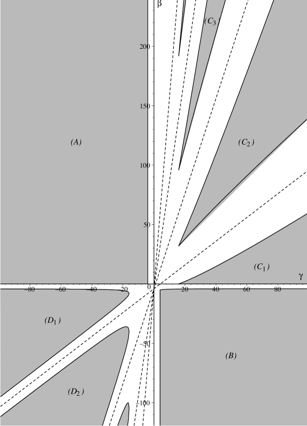
$$A=\{ (\gamma,\beta):\gamma\leq-4,\ \beta\geq 0\}$$

$$B=\{ (\gamma,\beta):\gamma\geq 4,\ \beta+4\leq-4/\gamma\}$$

$$C_{k}=\{ (\gamma,\beta):\gamma\geq 16,\ ((k-1)\sqrt{\gamma}+2)^{2}\leq\beta+4\leq(k\sqrt{\gamma}-2)^{2}\}$$

$$D_{k}=\{ (\gamma,\beta):\gamma\leq-16,$$

$$\frac{((2k-1)\sqrt{-\gamma}+\sqrt{-\gamma-16})^{2}}{-4}\leq\beta+4\leq\frac{((2k-1)\sqrt{-\gamma}-\sqrt{-\gamma-16})^{2}}{-4}\}$$

Dashed lines $\beta=k^{2}\gamma-4$, $k=1,2,3,\dots$

Figure 8. The discrete free groups

Finally, we are able to draw those subsets of $S_{\infty}$ that correspond to discrete free groups. These subsets are shown in Figure 8. The dashed lines $\beta=k^{2}\gamma-4$ are plotted to show a certain symmetry of $S_{\infty}$.

The other discrete groups contain elliptic elements. Their parameters are represented by lines, parabolas, hyperbolas, and points accumulating, as orders of elliptic elements tend to $\infty$, to the regions of free groups.

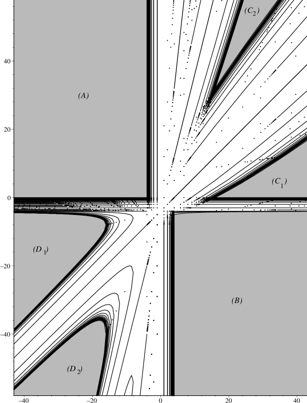
Figure 9. The structure of the slice $S_{\infty}$

In Figure 9, the whole picture for the slice $S_{\infty}$ is shown to give an idea of the structure of $S_{\infty}$. The formulas for $\beta$ and $\gamma$ obtained in Theorems 2.6, 4.4, 4.6, 4.8, and 4.9, were programmed with the package Maple 7.0 for some (sufficiently large) values of independent variables like $n,q\in{\mathbb{Z}}$ and $u,v\in\mathcal{U}$ and plotted on the plane $(\gamma,\beta)$.

The most interesting families of parameters appear when $\gamma$ and $\beta$ are of the same sign. For a fixed $k$, the hyperbolas

$$-4(\beta+4)=\left((2k-1)\sqrt{-\gamma}\pm\sqrt{-\gamma-8(1+\cos(\pi/p))}\right)^{2},$$

where $p\geq 2$ is an integer, form a one-parameter family of curves converging to the boundary of $D_{k}$ as $p\to\infty$. Each hyperbola has the asymptotes $\beta=(k-1)^{2}\gamma-4k(1+\cos(\pi/p))+4$ and $\beta=k^{2}\gamma+4k(1+\cos(\pi/p))-4$, which are obviously parallel to $\beta=(k-1)^{2}\gamma-4$ and $\beta=k^{2}\gamma-4$, respectively.

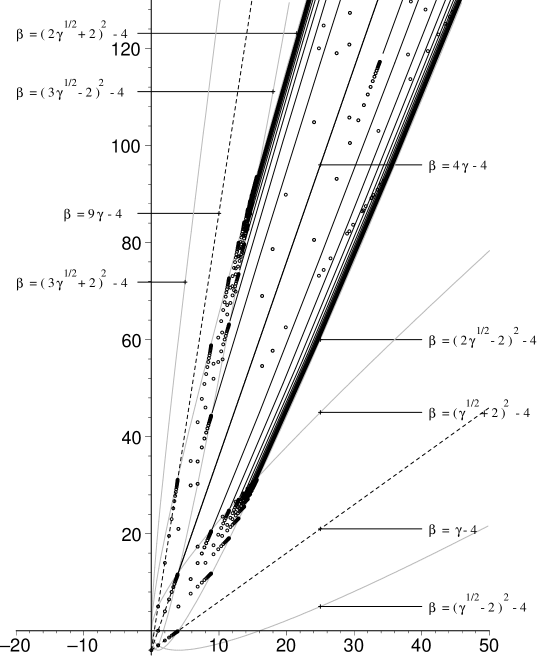
Figure 10. The structure of $\Sigma_{2}$

For $\gamma>0$ and $\beta>0$, consider a one-parameter family of parabolas $\beta_{k}=(k\sqrt{\gamma}\pm 2)^{2}-4$. Let $\Sigma_{k}$ be the domain bounded by $\beta_{k}$:

$$\Sigma_{k}=\{(\gamma,\beta):(k\sqrt{\gamma}-2)^{2}\leq\beta+4\leq(k\sqrt{\gamma}+2)^{2}\}.$$

Within each $\Sigma_{k}$, the parameters for discrete groups are given by

$$\left\{\begin{array}[]{l}\beta=(k\sqrt{\gamma}\pm 2\cos(q\pi/n))^{2}-4,\\ \gamma=4C(q,n)(\cos(\pi/n)+\cosh u)^{2},\end{array}\right.$$

where $(q,n)=1$, $1\leq q<n/2$, and $u\in\mathcal{U}$. Note that for $n=2$, we have $\beta=k^{2}\gamma-4$ and $\gamma=4\cosh^{2}u$. As $n\to\infty$, the curves $\beta=(k\sqrt{\gamma}\pm 2\cos(q\pi/n))^{2}-4$ accumulate to the boundary of $\Sigma_{k}$, i.e., to the boundaries of $C_{k-1}$ and $C_{k}$ (see Figure 10 for an example of $\Sigma_{k}$ for $k=2$).

References

- [1] A. F. Beardon, The geometry of discrete groups, Springer-Verlag, New York–Heidelberg–Berlin, 1983.
- [2] A. F. Beardon, Fuchsian groups and th roots of parabolic generators, Holomorphic functions and moduli, Vol. II (Berkeley, CA, 1986), 13–22, Math. Sci. Res. Inst. Publ., 11, 1988.
- [3] D. B. A. Epstein and C. Petronio, An exposition of Poincaré’s polyhedron theorem, L’Enseignement Mathématique 40 (1994), 113–170.
- [4] W. Fenchel, Elementary geometry in hyperbolic space, de Gruyter Studies in Mathematics, 11. Walter de Gruyter & Co., Berlin, 1989.
- [5] F. W. Gehring, J. P. Gilman, and G. J. Martin, Kleinian groups with real parameters, Commun. Contemp. Math. 3, no. 2 (2001), 163–186.
- [6] F. W. Gehring and G. J. Martin, Stability and extremality in Jørgensen’s inequality, Complex Variables Theory Appl. 12 (1989), no. 1-4, 277–282.
- [7] F. W. Gehring and G. J. Martin, Chebyshev polynomials and discrete groups, Proc. of the Conf. on Complex Analysis (Tianjin, 1992), 114–125, Conf. Proc. Lecture Notes Anal., I, Internat. Press, Cambridge, MA, 1994.
- [8] J. Gilman and B. Maskit, An algorithm for -generator Fuchsian groups, Mich. Math. J. 38 (1991), no. 1, 13–32.
- [9] E. Klimenko and N. Kopteva, Discreteness criteria for groups, Israel J. Math. 128 (2002), 247–265.
- [10] E. Klimenko and N. Kopteva, All discrete groups whose generators have real traces, Int. J. Algebra Comput. 15 (2005), no. 3, 577–618.
- [11] E. Klimenko and N. Kopteva, Discrete groups with a parabolic generator, Sib. Math. J. 46 (2005), no. 6, 1069–1076.
- [12] E. Klimenko and N. Kopteva, Two-generator Kleinian orbifolds, 2005, preprint.
- [13] E. Klimenko and M. Sakuma, Two-generator discrete subgroups of containing orientation-reversing elements, Geometriae Dedicata 72 (1998), 247–282.
- [14] A. W. Knapp, Doubly generated Fuchsian groups, Mich. Math. J. 15 (1968), no. 3, 289–304.
- [15] J. P. Matelski, The classification of discrete 2-generator subgroups of , Israel J. Math. 42 (1982), no. 4, 309–317.
- [16] E. B. Vinberg, Hyperbolic reflection groups, Russian Math. Surveys 40 (1985), 31–75.