[G-]parab-ortho1 [W-]eph-wheel

EPAL1: Geometry of Invariants

Erlangen Program at Large–1: Geometry of Invariants

Vladimir V. Kisil

V. V. Kisil

School of Mathematics, University of Leeds, Leeds LS2 9JT, UK
On leave from the Odessa University

kisilv@maths.leeds.ac.uk

http://www.maths.leeds.ac.uk/~kisilv/

Received April 20, 2010, in final form September 10, 2010; Published online September 26, 2010

This paper presents geometrical foundation for a systematic treatment of three main (elliptic, parabolic and hyperbolic) types of analytic function theories based on the representation theory of $SL_{2}{}(\mathbb{R}{})$ group. We describe here geometries of corresponding domains. The principal rôle is played by Clifford algebras of matching types. In this paper we also generalise the Schwerdtfeger–Fillmore–Springer–Cnops construction which describes cycles as points in the extended space. This allows to consider many algebraic and geometric invariants of cycles within the Erlangen program approach. analytic function theory, semisimple groups, elliptic, parabolic, hyperbolic, Clifford algebras, complex numbers, dual numbers, double numbers, split-complex numbers, Moebius transformations 30G35, 22E46, 30F45, 32F45

1 Introduction

This paper describes geometry of simples two-dimensional domains in the spirit of the Erlangen program of F. Klein influenced by works of S. Lie, for its development see books [BarkerHowe07] [Sharpe97] [RozenfeldZamakhovski03] and their references. Further works in this series will use the Erlangen approach for analytic function theories and spectral theory of operators [Kisil10b]. In the present paper we are focused on the geometry and study objects in a plane and their properties which are invariant under linear-fractional transformations associated to the $SL_{2}{}(\mathbb{R}{})$ group. The basic observation is that geometries obtained in this way are naturally classified as elliptic, parabolic and hyperbolic.

1.1 Background and History

We repeatedly meet such a division of various mathematical objects into three main classes. They are named by the historically first example—the classification of conic sections: elliptic, parabolic and hyperbolic—however the pattern persistently reproduces itself in many very different areas (equations, quadratic forms, metrics, manifolds, operators, etc.). We will abbreviate this separation as EPH-classification. The common origin of this fundamental division can be seen from the simple picture of a coordinate line split by the zero into negative and positive half-axes:

(1.1)

Connections between different objects admitting EPH-classification are not limited to this common source. There are many deep results linking, for example, ellipticity of quadratic forms, metrics and operators. On the other hand there are still a lot of white spots and obscure gaps between some subjects as well.

For example, it is well known that elliptic operators are effectively treated through complex analysis, which can be naturally identified as the elliptic analytic function theory [Kisil97c, Kisil01a]. Thus there is a natural quest for hyperbolic and parabolic analytic function theories, which will be of similar importance for corresponding types of operators. A search for hyperbolic function theory was attempted several times starting from 1930’s, see for example [VignauxDuranona35a, LavrentShabat77, MotterRosa98]. Despite of some important advances the obtained hyperbolic theory does not look as natural and complete as complex analysis is. Parabolic geometry was considered in an excellent book [Yaglom79], which is still a source of valuable inspirations. However the corresponding “parabolic calculus” described in various places [CatoniCannataNichelatti04] [Gromov90a] [Zejliger34] is rather trivial.

There is also a recent interest to this topic in different areas: differential geometry [BekkaraFrancesZeghib06, CatoniCannataNichelatti04, CatoniCannataZampetti05, FjelstadGal01, Benz07a, BairdWood09a], modal logic [KuruczWolterZakharyaschev05], quantum mechanics [Khrennikov05a, KhrennikovSegre07a, McRae07, Kisil10a], space-time geometry [BocCatoniCannataNichZamp07, HerranzSantander02b, HerranzSantander02a, Mirman01a, GromovKuratov05a, Garasko09a, Pavlov06a], hypercomplex analysis [CerejeirasKahlerSommen05a, EelbodeSommen04a, EelbodeSommen05a]. A brief history of the topic can be found in [CatoniCannataZampetti05] and further references are provided in the above papers.

Most of previous research had an algebraic flavour. An alternative approach to analytic function theories based on the representation theory of semisimple Lie groups was developed in the series of papers [Kisil95d, Kisil96d, Kisil96c, Kisil97c, Kisil94e, Kisil98a, Kisil01a]. Particularly, some elements of hyperbolic function theory were built in [Kisil96d, Kisil97c] along the same lines as the elliptic one—standard complex analysis. Covariant functional calculus of operators and respective covariant spectra were considered in [Kisil95i, Kisil02a].

This paper continues this line of research and significantly expands results of the earlier paper [Kisil04b], see also [Kisil06a] for an easy-reading introduction. A brief outline of the Erlangen Programme at Large, which includes geometry, analytic functions and functional calculus, is written in [Kisil10b].

1.2 Highlights of Obtained Results

In the previous paper [Kisil04b] we identify geometric objects called cycles [Yaglom79], which are circles, parabolas and hyperbolas in the corresponding EPH cases. They are invariants of the Möbius transformations, i.e. the natural geometric objects in the sense of the Erlangen program. Note also that cycles are algebraically defined through the quadratic expressions (2.10b) which may lead to interesting connections with the innovative approach to the geometry presented in [Wildberger05].

In this paper we systematically study those cycles through an essential extension of the Schwerdtfeger–Fillmore–Springer–Cnops construction [Schwerdtfeger79a, Cnops02a, Porteous95, FillmoreSpringer90a, Kirillov06, Kisil12a] abbreviated in this paper as SFSCc. The idea behind SFSCc is to consider cycles not as loci of points from the initial point space but rather as points of the new cycle space, see § 3.1. Then many geometrical properties of the point space may be better expressed through properties of the cycle space. Notably Möbius linear-fractional transformations of the point space are linearised in the cycle space, see Prop. 3.3.

An interesting feature of the correspondence between the point and cycle spaces is that many relations between cycles, which are of local nature in the cycle space, looks like non-local if translated back to the point space, see for example non-local character of cycle orthogonality in Fig. 8 and 10. Such a non-point behaviour is oftenly thought to be a characteristic property of non-commutative geometry but appears here within the Erlangen program approach [Kisil97a, Kisil02c]. This also demonstrates that our results cannot be reduced to the ordinary differential geometry or nine Cayley–Klein geometries of the plane [Yaglom79]*App. C [Pimenov65a].

Remark 1.1.

Introducing parabolic objects on a common ground with elliptic and hyperbolic ones we should warn against some common prejudices suggested by picture (1.1):

1. The parabolic case is unimportant (has “zero measure”) in comparison to the elliptic and hyperbolic ones. As we shall see (e.g. Remark 8.6 and 5.13.2) some geometrical features are richer in parabolic case.

2. The parabolic case is a limiting situation (a contraction) or an intermediate position between the elliptic and hyperbolic ones: all properties of the former can be guessed or obtained as a limit or an average from the latter two. Particularly this point of view is implicitly supposed in [LavrentShabat77].

   Although there are few confirmations of this (e.g. Fig. 17($E$)–($H$)), we shall see (e.g. Remark 5.29) that some properties of the parabolic case cannot be straightforwardly guessed from a combination of the elliptic and hyperbolic cases.

3. All three EPH cases are even less disjoint than it is usually thought. For example, there are meaningful notions of centre of a parabola (2.12) or focus of a circle (3.10).

4. A (co-)invariant geometry is believed to be “coordinate free” which sometimes is pushed to an absolute mantra. However our study within the Erlangen program framework reveals two useful notions (Defn. 2.12 and  (3.10)) mentioned above which are defined by coordinate expressions and look very “non-invariant” on the first glance.

An amazing aspect of this topic is a transparent similarity between all three EPH cases which is combined with some non-trivial exceptions like non-invariance of the upper half-plane in the hyperbolic case (subsection 7.2) or non-symmetric length and orthogonality in the parabolic case (Lemma 5.28.(p)). The elliptic case seems to be free from any such irregularities only because it is the standard model by which the others are judged.

Remark 1.2.

We should say a word or two on proofs in this paper. Majority of them are done through symbolic computations performed in the paper [Kisil05b] on the base of GiNaC [GiNaC] computer algebra system. As a result we can reduce many proofs just to a one-line reference to the paper [Kisil05b]. In a sense this is the complete fulfilment of the Cartesian program of reducing geometry to algebra with the latter to be done by straightforward mechanical calculations. Therefore the Erlangen program is nicely compatible with the Cartesian approach: the former defines the set of geometrical object with invariant properties and the latter provides a toolbox for their study. Another example of their unification in the field of non-commutative geometry was discussed in [Kisil02c].

However the lack of intelligent proofs based on smart arguments is undoubtedly a deficiency. An enlightening reasoning (e.g. the proof of Lem. 2.14) besides establishing the correctness of a mathematical statement gives valuable insights about deep relations between objects. Thus it will be worth to reestablish key results of this paper in a more synthetic way.

1.3 The Paper Outline

Section 2 describes the $SL_{2}{}(\mathbb{R}{})$ group, its one-dimensional subgroups and corresponding homogeneous spaces. Here corresponding Clifford algebras show their relevance and cycles naturally appear as $SL_{2}{}(\mathbb{R}{})$-invariant objects.

To study cycles we extend in Section 3 the Schwerdtfeger–Fillmore–Springer–Cnops construction (SFSCc) to include parabolic case. We also refine SFSCc from a traditional severe restriction that space of cycles posses the same metric as the initial point space. Cycles became points in a bigger space and got their presentation by matrix. We derive first $SL_{2}{}(\mathbb{R}{})$-invariants of cycles from the classic matrix invariants.

Mutual disposition of two cycles may be also characterised through an invariant notions of (normal and focal) orthogonalities, see Section 4, both are defined in matrix terms of SFSCc. Orthogonality in generalised SFSCc is not anymore a local property defined by tangents in the intersection point of cycles. Moreover, the focal orthogonality is not even symmetric. The corresponding notion of inversion (in a cycle) is considered as well.

Section 5 describes distances and lengths defined by cycles. Although they share some strange properties (e.g. non-local character or non-symmetry) with the orthogonalities they are legitimate objects in Erlangen approach since they are conformal under the Möbius maps. We also consider the corresponding perpendicularity and its relation to orthogonality. Invariance of “infinitesimal” cycles and corresponding version of conformality is considered in Section 6.

Section 7 deals with the global properties of the plane, e.g. its proper compactification by a zero-radius cycle at infinity. Finally, Section 8 considers some aspects of the Cayley transform, with nicely interplays with other notions (e.g. focal orthogonality, lengths, etc.) considered in the previous sections.

To finish this introduction we point out the following natural question.

Problem 1.3.

To which extend the subject presented here can be generalised to higher dimensions?

2 Elliptic, Parabolic and Hyperbolic Homogeneous Spaces

We begin from representations of the $SL_{2}{}(\mathbb{R}{})$ group in Clifford algebras with two generators. They naturally introduce circles, parabolas and hyperbolas as invariant objects of corresponding geometries.

2.1 $SL_{2}{}(\mathbb{R}{})$ group and Clifford Algebras

We consider Clifford algebras defined by elliptic, parabolic and hyperbolic bilinear forms. Then representations of $SL_{2}{}(\mathbb{R}{})$ defined by the same formula (2.3) will inherit this division.

Convention 2.1.

There will be three different Clifford algebras ${\mathcal{C}\kern-1.19995pt\ell(e)}$, ${\mathcal{C}\kern-1.19995pt\ell(p)}$, ${\mathcal{C}\kern-1.19995pt\ell(h)}$ corresponding to elliptic, parabolic, and hyperbolic cases respectively. The notation ${\mathcal{C}\kern-1.19995pt\ell(\sigma)}$, with assumed values $\sigma=-1$, $0$, $1$, refers to any of these three algebras.

A Clifford algebra ${\mathcal{C}\kern-1.19995pt\ell(\sigma)}$ as a $4$-dimensional linear space is spanned by $1$, $e_{0}$, $e_{1}$, $e_{0}e_{1}$ with non-commutative multiplication defined by the following identities:

$$e_{0}^{2}=-1,\qquad e_{1}^{2}=\sigma=\left\{\begin{array}[]{cl}-1,&\textrm{for ${\mathcal{C}\kern-1.19995pt\ell(e)}$---{elliptic} case}\\ 0,&\textrm{for ${\mathcal{C}\kern-1.19995pt\ell(p)}$---{parabolic} case}\\ 1,&\textrm{for ${\mathcal{C}\kern-1.19995pt\ell(h)}$---{hyperbolic} case}\\ \end{array}\right.,\qquad e_{0}e_{1}=-e_{1}e_{0}.$$ (2.1)

The two-dimensional subalgebra of ${\mathcal{C}\kern-1.19995pt\ell(e)}$ spanned by $1$ and $\mathrm{i}=e_{1}e_{0}=-e_{0}e_{1}$ is isomorphic (and can actually replace in all calculations!) the field of complex numbers $\mathbb{C}{}$. For example, from (2.1) follows that $\mathrm{i}^{2}=(e_{1}e_{0})^{2}=-1$. For any ${\mathcal{C}\kern-1.19995pt\ell(\sigma)}$ we identify $\mathbb{R}^{2}{}$ with the set of vectors $w=ue_{0}+ve_{1}$, where $(u,v)\in\mathbb{R}^{2}{}$. In the elliptic case of ${\mathcal{C}\kern-1.19995pt\ell(e)}$ this maps

$$(u,v)\mapsto e_{0}(u+\mathrm{i}v)=e_{0}z,\qquad\textrm{ with }z=u+\mathrm{i}v,$$ (2.2)

in the standard form of complex numbers. Similarly, see [Kisil06a] and [Yaglom79]*Supl. C

1. in the parabolic case $\varepsilon=e_{1}e_{0}$ (such that $\varepsilon^{2}=0$) is known as dual unit and all expressions $u+\varepsilon v$, $u,v\in\mathbb{R}{}$ form dual numbers.

2. in the hyperbolic case $e=e_{1}e_{0}$ (such that $e^{2}=1$) is known as double unit and all expressions $u+ev$, $u,v\in\mathbb{R}{}$ constitute double numbers.

Remark 2.1.

A part of this paper can be rewritten in terms of complex, dual and double numbers and it will have some common points with Supplement C of the book [Yaglom79]. However the usage of Clifford algebras provides some facilities which do not have natural equivalent in complex numbers, see Rem. 4.17. Moreover the language of Clifford algebras is more uniform and also allows straightforward generalisations to higher dimensions [Kisil96d].

We denote the space $\mathbb{R}^{2}{}$ of vectors $ue_{0}+ve_{1}$ by $\mathbb{R}^{e}{}$, $\mathbb{R}^{p}{}$ or $\mathbb{R}^{h}{}$ to highlight which of Clifford algebras is used in the present context. The notation $\mathbb{R}^{\sigma}{}$ assumes ${\mathcal{C}\kern-1.19995pt\ell(\sigma)}$.

The $SL_{2}{}(\mathbb{R}{})$ group [HoweTan92, Lang85, MTaylor86] consists of $2\times 2$ matrices

$$\begin{pmatrix}a&b\\ c&d\end{pmatrix},\qquad\textrm{ with }a,b,c,d\in\mathbb{R}{}\textrm{ and the determinant }ad-bc=1.$$

An isomorphic realisation of $SL_{2}{}(\mathbb{R}{})$ with the same multiplication is obtained if we replace a matrix $\begin{pmatrix}a&b\\ c&d\end{pmatrix}$ by $\begin{pmatrix}a&be_{0}\\ -ce_{0}&d\end{pmatrix}$ within any ${\mathcal{C}\kern-1.19995pt\ell(\sigma)}$. The advantage of the latter form is that we can define the Möbius transformation of $\mathbb{R}^{\sigma}{}\rightarrow\mathbb{R}^{\sigma}{}$ for all three algebras ${\mathcal{C}\kern-1.19995pt\ell(\sigma)}$ by the same expression:

$$\begin{pmatrix}a&be_{0}\\ -ce_{0}&d\end{pmatrix}:\ ue_{0}+ve_{1}\ \mapsto\ \frac{a(ue_{0}+ve_{1})+be_{0}}{-ce_{0}(ue_{0}+ve_{1})+d},$$ (2.3)

where the expression $\frac{a}{b}$ in a non-commutative algebra is always understood as $ab^{-1}$, see [Cnops94a, Cnops02a]. Therefore $\frac{ac}{bc}=\frac{a}{b}$ but $\frac{ca}{cb}\neq\frac{a}{b}$ in general.

Again in the elliptic case the transformation (2.3) is equivalent to, cf. [Beardon05a]*Ch. 13 [Beardon95]*Ch. 3:

$$\begin{pmatrix}a&be_{0}\\ -ce_{0}&d\end{pmatrix}:\ e_{0}z\ \mapsto\ \frac{e_{0}(a(u+e_{1}e_{0}v)+b)}{c(u+e_{1}e_{0}v)+d}=e_{0}\frac{az+b}{cz+d},\textrm{ where }z=u+\mathrm{i}v,$$

which is the standard form of a Möbius transformation. One can straightforwardly verify that the map (2.3) is a left action of $SL_{2}{}(\mathbb{R}{})$ on $\mathbb{R}^{\sigma}{}$, i.e. $g_{1}(g_{2}w)=(g_{1}g_{2})w$.

To study finer structure of Möbius transformations it is useful to decompose an element $g$ of $SL_{2}{}(\mathbb{R}{})$ into the product $g=g_{a}g_{n}g_{k}$:

$$\begin{pmatrix}a&be_{0}\\ -ce_{0}&d\end{pmatrix}={\begin{pmatrix}\alpha^{-1}&0\\ 0&\alpha\end{pmatrix}}{\begin{pmatrix}1&\nu e_{0}\\ 0&1\end{pmatrix}}{\begin{pmatrix}\cos\phi&e_{0}\sin\phi\\ e_{0}\sin\phi&\cos\phi\end{pmatrix}},$$ (2.4)

where the values of parameters are as follows:

$$\alpha=\sqrt{c^{2}+d^{2}},\qquad\nu=ac+bd,\qquad\phi=-\arctan\frac{c}{d}.$$ (2.5)

Consequently $\cos\phi=\frac{d}{\sqrt{c^{2}+d^{2}}}$ and $\sin\phi=\frac{-c}{\sqrt{c^{2}+d^{2}}}$. The product (2.4) gives a realisation of the Iwasawa decomposition  [Lang85]*§ III.1 in the form $SL_{2}{}(\mathbb{R}{})=ANK$, where $K$ is the maximal compact group, $N$ is nilpotent and $A$ normalises $N$.

2.2 Actions of Subgroups

We describe here orbits of the three subgroups from the Iwasawa decomposition (2.4) for all three types of Clifford algebras. However there are less than nine ($=3\times 3$) different orbits since in all three EPH cases the subgroups $A$ and $N$ act through Möbius transformation uniformly:

Lemma 2.2.

For any type of the Clifford algebra ${\mathcal{C}\kern-1.19995pt\ell(\sigma)}$:

1. The subgroup $N$ defines shifts $ue_{0}+ve_{1}\mapsto(u+\nu)e_{0}+ve_{1}$ along the “real” axis $U$ by $\nu$.
   The vector field of the derived representation is $dN_{a}{(u,v)}=(1,0)$.

2. The subgroup $A$ defines dilations $ue_{0}+ve_{1}\mapsto\alpha^{-2}(ue_{0}+ve_{1})$ by the factor $\alpha^{-2}$ which fixes origin $(0,0)$.
   The vector field of the derived representation is $dA_{a}{(u,v)}=(2u,2v)$.

Orbits and vector fields corresponding to the derived representation [Kirillov76]*§ 6.3 [Lang85]*Chap. VI of the Lie algebra $\mathfrak{sl}_{2}$ for subgroups $A$ and $N$ are shown in Fig. 1. Thin transverse lines join points of orbits corresponding to the same values of the parameter along the subgroup.

Figure 1: Actions of the subgroups $A$ and $N$ by Möbius transformations.

By contrast the actions of the subgroup $K$ look differently between the EPH cases, see Fig. 2. They obviously correlate with names chosen for ${\mathcal{C}\kern-1.19995pt\ell(e)}$, ${\mathcal{C}\kern-1.19995pt\ell(p)}$, ${\mathcal{C}\kern-1.19995pt\ell(h)}$. However algebraic expressions for these orbits are uniform.

Vector fields are:

$\begin{array}[]{rcll}dK_{e}(u,v)&=&(1+u^{2}-v^{2},&2uv)\\ dK_{p}(u,v)&=&(1+u^{2},&2uv)\\ dK_{h}(u,v)&=&(1+u^{2}+v^{2},&2uv)\\ \end{array}$

Figure 2: Action of the $K$ subgroup. The corresponding orbits are circles, parabolas and hyperbolas.

Lemma 2.3.

A $K$-orbit in $\mathbb{R}^{\sigma}{}$ passing the point $(0,t)$ has the following equation:

$$(u^{2}-\sigma v^{2})-2v\frac{t^{-1}-\sigma t}{2}+1=0,\qquad\text{where }\sigma=e_{1}^{2}\ (\textrm{i.e }-1,0\textrm{ or }1).$$ (2.6)

The curvature of a $K$-orbit at point $(0,t)$ is equal to

$$\kappa=\frac{2t}{1+\sigma t^{2}}.$$

A proof will be given later (see Ex. 3.5.2), when a more suitable tool will be in our disposal. Meanwhile these formulae allows to produce geometric characterisation of $K$-orbits.

Lemma 2.4.

1. For ${\mathcal{C}\kern-1.19995pt\ell(e)}$ the orbits of $K$ are circles, they are coaxal [CoxeterGreitzer]*§ 2.3 with the real line being the radical axis. A circle with centre at $(0,(v+v^{-1})/2)$ passing through two points $(0,v)$ and $(0,v^{-1})$.
   The vector field of the derived representation is $dK_{e}{(u,v)}=(u^{2}-v^{2}+1,2uv)$.

2. For ${\mathcal{C}\kern-1.19995pt\ell(p)}$ the orbits of $K$ are parabolas with the vertical axis $V$. A parabola passing through $(0,v/2)$ has horizontal directrix passing through $(0,v-v^{-1}/2)$ and focus at $(0,(v+v^{-1})/2)$.
   The vector field of the derived representation is $dK_{p}{(u,v)}=(u^{2}+1,2uv)$.

3. For ${\mathcal{C}\kern-1.19995pt\ell(h)}$ the orbits of $K$ are hyperbolas with asymptotes parallel to lines $u=\pm v$. A hyperbola passing through the point $(0,v)$ has the focal distance $2p$, where $p=\frac{v^{2}+1}{\sqrt{2}v}$ and the upper focus is located at $(0,f)$ with:

   $$f=\left\{\begin{array}[]{ll}p-\sqrt{\frac{p^{2}}{2}-1},&\textrm{ for }0<v<1;\textrm{ and }\\ p+\sqrt{\frac{p^{2}}{2}-1},&\textrm{ for }v\geq 1.\end{array}\right.$$

   The vector field of the derived representation is $dK_{h}{(u,v)}=(u^{2}+v^{2}+1,2uv)$.

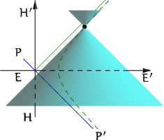
(a) (b)

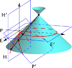
Figure 3: $K$-orbits as conic sections:
(a) a flat projection along $U$ axis;
(b) same values of $\phi$ on different orbits belong to the same generator of the cone.

Since all $K$-orbits are conic sections it is tempting to obtain them as sections of some cones. To this end we define the family of double-sided right-angle cones be parametrised by $t>0$:

$$x^{2}+(y-{\textstyle\frac{1}{2}}(t+t^{-1}))^{2}-(z-{\textstyle\frac{1}{2}}(t-t^{-1}))^{2}=0.$$ (2.7)

The vertices of cones belong to the hyperbola $\{x=0,y^{2}-z^{2}=1\}$, see Fig. 3 for illustration.

Lemma 2.5.

$K$-orbits may be obtained cases as follows:

1. elliptic $K$-orbits are sections of cones (2.7) by the plane $z=0$ ($EE^{\prime}$ on Fig. 3);

2. parabolic $K$-orbits are sections of (2.7) by the plane $y=\pm z$ ($PP^{\prime}$ on Fig. 3);

3. hyperbolic $K$-orbits are sections of (2.7) by the plane $y=0$ ($HH^{\prime}$ on Fig. 3);

Moreover, each straight line generating a cone from the family (2.7) is crossing corresponding elliptic, parabolic and hyperbolic $K$-orbits at points with the same value of parameter $\phi$ (2.5) of the subgroup $K$.

From the above algebraic and geometric descriptions of the orbits we can make several observations.

Remark 2.6.

1. The values of all three vector fields $dK_{e}$, $dK_{p}$ and $dK_{h}$ coincide on the “real” $U$-axis $v=0$, i.e. they are three different extensions into the domain of the same boundary condition. Another source of this: the axis $U$ is the intersection of planes $EE^{\prime}$, $PP^{\prime}$ and $HH^{\prime}$ on Fig. 3.

2. The hyperbola passing through the point $(0,1)$ has the shortest focal length $\sqrt{2}$ among all other hyperbolic orbits since it is the section of the cone $x^{2}+(y-1)^{2}+z^{2}=0$ closest from the family to the plane $HH^{\prime}$.

3. Two hyperbolas passing through $(0,v)$ and $(0,v^{-1})$ have the same focal length since they are sections of two cones with the same distance from $HH^{\prime}$. Moreover, two such hyperbolas in the lower- and upper half-planes passing the points $(0,v)$ and $(0,-v^{-1})$ are sections of the same double-sided cone. They are related to each other as explained in Remark 7.4.1.

One can see from the first picture in Fig. 2 that the elliptic action of subgroup $K$ fixes the point $e_{1}$. More generally we have:

Figure 4: Actions of the subgroups which fix point $e_{1}$ in three cases.

Lemma 2.7.

The fix group of the point $e_{1}$ is

1. the subgroup $K^{\prime}_{e}=K$ in the elliptic case. Thus the elliptic upper half-plane is a model for the homogeneous space $SL_{2}{}(\mathbb{R}{})/K$;

2. the subgroup $N^{\prime}_{p}$ of matrices

   $$\begin{pmatrix}1&0\\ \nu e_{0}&1\end{pmatrix}=\begin{pmatrix}0&e_{0}\\ e_{0}&0\end{pmatrix}\begin{pmatrix}1&\nu e_{0}\\ 0&1\end{pmatrix}\begin{pmatrix}0&-e_{0}\\ -e_{0}&0\end{pmatrix}$$ (2.8)

   in the parabolic case. It also fixes any point $ve1$. It is conjugate to subgroup $N$, thus the parabolic upper half-plane is a model for the homogeneous space $SL_{2}{}(\mathbb{R}{})/N$;

3. the subgroup $A^{\prime}_{h}$ of matrices

   $$\begin{pmatrix}\cosh(\tau)&\sinh(\tau)e_{0}\\ -\sinh(\tau)e_{0}&\cosh(\tau)\end{pmatrix}=\frac{1}{2}\begin{pmatrix}1&-e_{0}\\ -e_{0}&1\end{pmatrix}\begin{pmatrix}e^{\tau}&0\\ 0&e^{-\tau}\end{pmatrix}\begin{pmatrix}1&e_{0}\\ e_{0}&1\end{pmatrix},$$ (2.9)

   in the hyperbolic case. It is conjugate to subgroup $A$, thus two copies of the upper halfplane (see Section 7.2) is a model for $SL_{2}{}(\mathbb{R}{})/A$.

Moreover, vectors fields of these actions are $(u^{2}+\sigma(v^{2}-1),2uv)$ for the corresponding values of $\sigma$. Orbits of the fix groups satisfy to the equation:

$$(u^{2}-\sigma v^{2})-2lv-\sigma=0,\qquad\text{where }l\in\mathbb{R}{}.$$

Remark 2.8.

1. Note that we can uniformly express the fix-subgroups of $e_{1}$ in all EPH cases by matrices of the form:

   $$\begin{pmatrix}a&-\sigma e_{0}b\\ -e_{0}b&a\end{pmatrix},\qquad\text{ where }a^{2}-\sigma b^{2}=1.$$

2. In the hyperbolic case the subgroup $A^{\prime}_{h}$ may be extended to a subgroup $A^{\prime\prime}_{h}$ by the element $\begin{pmatrix}0&e_{0}\\ e_{0}&0\end{pmatrix}$, which flips upper and lower half-planes (see Section 7.2). The subgroup $A^{\prime\prime}_{h}$ fixes the set $\{e_{1},-e_{1}\}$.

Lemma 2.9.

Möbius action of $SL_{2}{}(\mathbb{R}{})$ in each EPH case is generated by action the corresponding fix-subgroup ($A^{\prime\prime}_{h}$ in the hyperbolic case) and actions of the $ax+b$ group, e.g. subgroups $A$ and $N$.

Proof 2.10.

The $ax+b$ group transitively acts on the upper or lower half-plane. Thus for any $g\in SL_{2}{}(\mathbb{R}{})$ there is $h$ in $ax+b$ group such that $h^{-1}g$ either fixes $e_{1}$ or sends it to $-e_{1}$. Thus $h^{-1}g$ is in the corresponding fix-group.

2.3 Invariance of Cycles

As we will see soon the three types of $K$-orbits are principal invariants of the constructed geometries, thus we will unify them in the following definition.

Definition 2.11.

We use the word cycle to denote loci in $\mathbb{R}^{\sigma}{}$ defined by the equation:

$$-k(ue_{0}+ve_{1})^{2}-2\left\langle(l,n),(u,v)\right\rangle+m=0$$ (2.10a)

or equivalently (avoiding any reference to Clifford algebra generators):

$$k(u^{2}-\sigma v^{2})-2lu-2nv+m=0,\qquad\text{ where }\sigma=e_{1}^{2},$$ (2.10b)

or equivalently (using only Clifford algebra operations, cf. [Yaglom79]*Supl. C(42a)):

$$Kw^{2}+Lw-wL+M=0,$$ (2.10c)

where $$w=ue_{0}+ve_{1} K=-ke_{01} L=-ne_{0}+le_{1} M=me_{01}$$, , , .

Such cycles obviously mean for certain $k$, $l$, $n$, $m$ straight lines and one of the following:

1. in the elliptic case: circles with centre $\left(\frac{l}{k},\frac{n}{k}\right)$ and squared radius $m-\frac{l^{2}+n^{2}}{k}$;

2. in the parabolic case: parabolas with horizontal directrix and focus at $\left(\frac{l}{k},\frac{m}{2n}-\frac{l^{2}}{2nk}+\frac{n}{2k}\right)$;

3. in the hyperbolic case: rectangular hyperbolas with centre $\left(\frac{l}{k},-\frac{n}{k}\right)$ and a vertical axis of symmetry.

Moreover words parabola and hyperbola in this paper always assume only the above described types. Straight lines are also called flat cycles.

All three EPH types of cycles are enjoying many common properties, sometimes even beyond that we normally expect. For example, the following definition is quite intelligible even when extended from the above elliptic and hyperbolic cases to the parabolic one.

Definition 2.12.

$\mathring{\sigma}$-Centre of the $\sigma$-cycle (2.10) for any EPH case is the point $\left(\frac{l}{k},-\mathring{\sigma}\frac{n}{k}\right)\in\mathbb{R}^{\sigma}{}$. Notions of e-centre, p-centre, h-centre are used along the adopted EPH notations.

Centres of straight lines are at infinity, see subsection 7.1.

Remark 2.13.

Here we use a signature $\mathring{\sigma}=-1$, $0$ or $1$ of a Clifford algebra which is not related to the signature $\sigma$ of the space $\mathbb{R}^{\sigma}{}$. We will need also a third signature $\breve{\sigma}$ to describe the geometry of cycles in Defn. 3.1.

The meaningfulness of this definition even in the parabolic case is justified, for example, by:

• the uniformity of description of relations between centres of orthogonal cycles, see the next subsection and Fig. 8.

• the appearance of concentric parabolas in Fig. 17($N_{P_{e}}$) and ($N_{P_{h}}$).

Using the Lemmas 2.2 and 2.4 we can give an easy (and virtually calculation-free!) proof of invariance for corresponding cycles.

Lemma 2.14.

Möbius transformations preserve the cycles in the upper half-plane, i.e.:

1. For ${\mathcal{C}\kern-1.19995pt\ell(e)}$ Möbius transformations map circles to circles.

2. For ${\mathcal{C}\kern-1.19995pt\ell(p)}$ Möbius transformations map parabolas to parabolas.

3. For ${\mathcal{C}\kern-1.19995pt\ell(h)}$ Möbius transformations map hyperbolas to hyperbolas.

Proof 2.15.

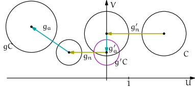
Figure 5: Decomposition of an arbitrary Möbius transformation $g$ into a product $g=g_{a}g_{n}g_{k}g_{a}^{\prime}g_{n}^{\prime}$.

Our first observation is that the subgroups $A$ and $N$ obviously preserve all circles, parabolas, hyperbolas and straight lines in all ${\mathcal{C}\kern-1.19995pt\ell(\sigma)}$. Thus we use subgroups $A$ and $N$ to fit a given cycle exactly on a particular orbit of subgroup $K$ shown on Fig. 2 of the corresponding type.

To this end for an arbitrary cycle $S$ we can find $g_{n}^{\prime}\in N$ which puts centre of $S$ on the $V$-axis, see Fig. 5. Then there is a unique $g_{a}^{\prime}\in A$ which scales it exactly to an orbit of $K$, e.g. for a circle passing through points $(0,v_{1})$ and $(0,v_{2})$ the scaling factor is $\frac{1}{\sqrt{v_{1}v_{2}}}$ according to Lemma 2.4.(e). Let $g^{\prime}=g_{a}^{\prime}g_{n}^{\prime}$, then for any element $g\in SL_{2}{}(\mathbb{R}{})$ using the Iwasawa decomposition of $gg^{\prime-1}=g_{a}g_{n}g_{k}$ we get the presentation $g=g_{a}g_{n}g_{k}g_{a}^{\prime}g_{n}^{\prime}$ with $g_{a},g_{a}^{\prime}\in A$, $g_{n},g_{n}^{\prime}\in N$ and $g_{k}\in K$.

Then the image $g^{\prime}S$ of the cycle $S$ under $g^{\prime}=g_{a}^{\prime}g_{n}^{\prime}$ is a cycle itself in the obvious way, then $g_{k}(g^{\prime}S)$ is again a cycle since $g^{\prime}S$ was arranged to coincide with a $K$-orbit, and finally $gS=g_{a}g_{n}(g_{k}(g^{\prime}S))$ is a cycle due to the obvious action of $g_{a}g_{n}$, see Fig. 5 for an illustration.

One can naturally wish that all other proofs in this paper will be of the same sort. This is likely to be possible, however we use a lot of computer algebra calculations as well.

3 Space of Cycles

We saw in the previous sections that cycles are Möbius invariant, thus they are natural objects of the corresponding geometries in the sense of F. Klein. An efficient tool of their study is to represent all cycles in $\mathbb{R}^{\sigma}{}$ by points of a new bigger space.

3.1 Schwerdtfeger–Fillmore–Springer–Cnops Construction (SFSCc)

It is well known that linear-fractional transformations can be linearised by a transition into a suitable projective space [Olver99]*Cha. 1. The fundamental idea of the Schwerdtfeger–Fillmore–Springer–Cnops construction (SFSCc) [Schwerdtfeger79a, Cnops02a, Porteous95, FillmoreSpringer90a, Kirillov06, Kisil12a] is that for linearisation of Möbius transformation in $\mathbb{R}^{\sigma}{}$ the required projective space can be identified with the space of all cycles in $\mathbb{R}^{\sigma}{}$. The latter can be associated with certain subset of $2\times 2$ matrices. SFSCc can be adopted from [Cnops02a, Porteous95] to serve all three EPH cases with some interesting modifications.

Definition 3.1.

Let $\mathbb{P}^{3}{}$ be the projective space, i.e. collection of the rays passing through points in $\mathbb{R}^{4}{}$. We define the following two identifications (depending from some additional parameters $\sigma$, $\breve{\sigma}$ and $s$ described below) which map a point $(k,l,n,m)\in\mathbb{P}^{3}{}$ to:

• the cycle (quadric) ${C}$ on $\mathbb{R}^{\sigma}{}$ defined by the equations (2.10) with constant parameters $k$, $l$, $n$, $m$:

  $$-k(e_{0}u+e_{1}v)^{2}-2\left\langle(l,n),(u,v)\right\rangle+m=0,$$ (3.1)

  for some ${\mathcal{C}\kern-1.19995pt\ell(\sigma)}$ with generators $e_{0}^{2}=-1$, $e_{1}^{2}=\sigma$.

• the ray of $2\times 2$ matrices passing through

  $${C^{s}_{\breve{\sigma}}}=\begin{pmatrix}l\breve{e}_{0}+sn\breve{e}_{1}&m\\ k&-l\breve{e}_{0}-sn\breve{e}_{1}\end{pmatrix}\in M_{2}({\mathcal{C}\kern-1.19995pt\ell(\breve{\sigma})}),\text{ with }\breve{e}_{0}^{2}=-1,\breve{e}_{1}^{2}=\breve{\sigma},$$ (3.2)

  i.e. generators $\breve{e}_{0}$ and $\breve{e}_{1}$ of ${\mathcal{C}\kern-1.19995pt\ell(\breve{\sigma})}$ can be of any type: elliptic, parabolic or hyperbolic regardless of the ${\mathcal{C}\kern-1.19995pt\ell(\sigma)}$ in (3.1).

The meaningful values of parameters $\sigma$, $\breve{\sigma}$ and $s$ are $-1$, $0$ or $1$, and in many cases $s$ is equal to $\sigma$.

Remark 3.2.

A hint for the composition of the matrix (3.2) is provided by the following identity:

$$\begin{pmatrix}1&w\end{pmatrix}\begin{pmatrix}L&M\\ K&-L\end{pmatrix}\begin{pmatrix}w\\ 1\end{pmatrix}=wKw+Lw-wL+M,$$

which realises the equation (2.10c) of a cycle.

The both identifications $Q$ and $M$ are straightforward. Indeed, a point $(k,l,n,m)\in\mathbb{P}^{3}{}$ equally well represents (as soon as $\sigma$, $\breve{\sigma}$ and $s$ are already fixed) both the equation (3.1) and the ray of matrix (3.2). Thus for fixed $\sigma$, $\breve{\sigma}$ and $s$ one can introduce the correspondence between quadrics and matrices shown by the horizontal arrow on the following diagram:

(3.3)

which combines $Q$ and $M$. On the first glance the dotted arrow seems to be of a little practical interest since it depends from too many different parameters ($\sigma$, $\breve{\sigma}$ and $s$). However the following result demonstrates that it is compatible with easy calculations of images of cycles under the Möbius transformations.

Proposition 3.3.

A cycle $-k(e_{0}u+e_{1}v)^{2}-2\left\langle(l,n),(u,v)\right\rangle+m=0$ is transformed by $g\in SL_{2}{}(\mathbb{R}{})$ into the cycle $-\tilde{k}(e_{0}u+e_{1}v)^{2}-2\left\langle(\tilde{l},\tilde{n}),(u,v)\right\rangle+\tilde{m}=0$ such that

$${\tilde{C}^{s}_{\breve{\sigma}}}=g{C^{s}_{\breve{\sigma}}}g^{-1}$$ (3.4)

for any Clifford algebras ${\mathcal{C}\kern-1.19995pt\ell(\sigma)}$ and ${\mathcal{C}\kern-1.19995pt\ell(\breve{\sigma})}$. Explicitly this means:

$$\begin{pmatrix}\tilde{l}\breve{e}_{0}+s\tilde{n}\breve{e}_{1}&\tilde{m}\\ \tilde{k}&-\tilde{l}\breve{e}_{0}-s\tilde{n}\breve{e}_{1}\end{pmatrix}$$

$$= \begin{pmatrix}a&b\breve{e}_{0}\\ -c\breve{e}_{0}&d\end{pmatrix}\begin{pmatrix}l\breve{e}_{0}+sn\breve{e}_{1}&m\\ k&-l\breve{e}_{0}-sn\breve{e}_{1}\end{pmatrix}\begin{pmatrix}d&-b\breve{e}_{0}\\ c\breve{e}_{0}&a\end{pmatrix}.$$

Proof 3.4.

It is already established in the elliptic and hyperbolic cases for $\sigma=\breve{\sigma}$, see [Cnops02a]. For all EPH cases (including parabolic) it can be done by the direct calculation in GiNaC [Kisil05b]*§ LABEL:G-sec:mobi-invar-cycl. An alternative idea of an elegant proof based on the zero-radius cycles and orthogonality (see below) may be borrowed from [Cnops02a].

Example 3.5.

1. The real axis $v=0$ is represented by the ray coming through $(0,0,1,0)$ and a matrix $\begin{pmatrix}s\breve{e}_{1}&0\\ 0&-s\breve{e}_{1}\end{pmatrix}$. For any $\begin{pmatrix}a&b\breve{e}_{0}\\ -c\breve{e}_{0}&d\end{pmatrix}\in SL_{2}{}(\mathbb{R}{})$ we have:

   $$\begin{pmatrix}a&b\breve{e}_{0}\\ -c\breve{e}_{0}&d\end{pmatrix}\begin{pmatrix}s\breve{e}_{1}&0\\ 0&-s\breve{e}_{1}\end{pmatrix}\begin{pmatrix}d&-b\breve{e}_{0}\\ c\breve{e}_{0}&a\end{pmatrix}=\begin{pmatrix}s\breve{e}_{1}&0\\ 0&-s\breve{e}_{1}\end{pmatrix},$$

   i.e. the real line is $SL_{2}{}(\mathbb{R}{})$-invariant.

2. A direct calculation in GiNaC [Kisil05b]*§ LABEL:G-sec:transf-k-orbits shows that matrices representing cycles from (2.6) are invariant under the similarity with elements of $K$, thus they are indeed $K$-orbits.

It is surprising on the first glance that the ${C^{s}_{\breve{\sigma}}}$ is defined through a Clifford algebra ${\mathcal{C}\kern-1.19995pt\ell(\breve{\sigma})}$ with an arbitrary sign of $\breve{e}_{1}^{2}$. However a moment of reflections reveals that transformation (3.3) depends only from the sign of $\breve{e}_{0}^{2}$ but does not involve any quadratic (or higher) terms of $\breve{e}_{1}$.

Remark 3.6.

Such a variety of choices is a consequence of the usage of $SL_{2}{}(\mathbb{R}{})$—a smaller group of symmetries in comparison to the all Möbius maps of $\mathbb{R}^{2}{}$. The $SL_{2}{}(\mathbb{R}{})$ group fixes the real line and consequently a decomposition of vectors into “real” ($e_{0}$) and “imaginary” ($e_{1}$) parts is obvious. This permits to assign an arbitrary value to the square of the “imaginary unit” $e_{1}e_{0}$.

Geometric invariants defined below, e.g. orthogonalities in sections 4.1 and 4.3, demonstrate “awareness” of the real line invariance in one way or another. We will call this the boundary effect in the upper half-plane geometry. The famous question on hearing drum’s shape has a sister:

Can we see/feel the boundary from inside a domain?

Rems. 3.14, 4.13 and 4.28 provide hints for positive answers.

(a) (b)

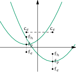
Figure 6: (a) Different EPH implementations of the same cycles defined by quadruples of numbers.
(b) Centres and foci of two parabolas with the same focal length.

To encompass all aspects from (3.3) we think a cycle ${C^{s}_{\breve{\sigma}}}$ defined by a quadruple $(k,l,n,m)$ as an “imageless” object which have distinct implementations (a circle, a parabola or a hyperbola) in the corresponding space $\mathbb{R}^{\sigma}{}$. These implementations may look very different, see Fig. 6(a), but still have some properties in common. For example,

• All implementations have the same vertical axis of symmetries;

• Intersections with the real axis (if exist) coincide, see $r_{1}$ and $r_{2}$ for the left cycle in Fig. 6(a).

• Centres of circle $c_{e}$ and corresponding hyperbolas $c_{h}$ are mirror reflections of each other in the real axis with the parabolic centre be in the middle point.

Lemma 2.4 gives another example of similarities between different implementations of the same cycles defined by the equation (2.6).

Finally, we may restate the Prop. 3.3 as an intertwining property.

Corollary 3.7.

Any implementation of cycles shown on (3.3) by the dotted arrow for any combination of $\sigma$, $\breve{\sigma}$ and $s$ intertwines two actions of $SL_{2}{}(\mathbb{R}{})$: by matrix conjugation (3.4) and Möbius transformations (2.3).

Remark 3.8.

A similar representation of circles by $2\times 2$ complex matrices which intertwines Möbius transformations and matrix conjugations was used recently by A.A. Kirillov [Kirillov06] in the study of the Apollonian gasket. Kirillov’s matrix realisation [Kirillov06] of a cycle has an attractive “self-adjoint” form:

$${C^{s}_{\breve{\sigma}}}=\begin{pmatrix}m&l\breve{e}_{0}+sn\breve{e}_{1}\\ -l\breve{e}_{0}-sn\breve{e}_{1}&k\end{pmatrix}\text{ (in notations of this paper)}.$$ (3.6)

Note that the matrix inverse to (3.6) is intertwined with the SFSCc presentation (3.2) by the matrix $\begin{pmatrix}0&1\\ 1&0\end{pmatrix}$.

3.2 First Invariants of Cycles

Using implementations from Definition 3.1 and relation (3.4) we can derive some invariants of cycles (under the Möbius transformations) from well-known invariants of matrix (under similarities). First we use trace to define an invariant inner product in the space of cycles.

Definition 3.9.

Inner $\breve{\sigma}$-product of two cycles is given by the trace of their product as matrices:

$$\left\langle{C^{s}_{\breve{\sigma}}},{\tilde{C}^{s}_{\breve{\sigma}}}\right\rangle=\mathop{tr}({C^{s}_{\breve{\sigma}}}{\tilde{C}^{s}_{\breve{\sigma}}}).$$ (3.7)

The above definition is very similar to an inner product defined in operator algebras [Arveson76]. This is not a coincidence: cycles act on points of $\mathbb{R}^{\sigma}{}$ by inversions, see subsection 4.2, and this action is linearised by SFSCc, thus cycles can be viewed as linear operators as well.

Geometrical interpretation of the inner product will be given in Cor. 5.9.

An obvious but interesting observation is that for matrices representing cycles we obtain the second classical invariant (determinant) under similarities (3.4) from the first (trace) as follows:

$$\left\langle{C^{s}_{\breve{\sigma}}},{C^{s}_{\breve{\sigma}}}\right\rangle=-2\det{C^{s}_{\breve{\sigma}}}.$$ (3.8)

The explicit expression for the determinant is:

$$\det{C^{s}_{\breve{\sigma}}}=l^{2}-\breve{\sigma}s^{2}n^{2}-mk$$ (3.9)

We recall that the same cycle is defined by any matrix $\lambda{C^{s}_{\breve{\sigma}}}$, $\lambda\in\mathbb{R}_{+}{}$, thus the determinant, even being Möbius-invariant, is useful only in the identities of the sort $\det{C^{s}_{\breve{\sigma}}}=0$. Note also that $\mathop{tr}({C^{s}_{\breve{\sigma}}})=0$ for any matrix of the form (3.2). Since it may be convenient to have a predefined representative of a cycle out of the ray of equivalent SFSCc matrices we introduce the following normalisation.

Definition 3.10.

A SFSCc matrix representing a cycle is said to be $k$-normalised if its $(2,1)$-element is $1$ and it is $\det$-normalised if its determinant is equal $1$.

Each normalisation has its own advantages: element $(1,1)$ of $k$-normalised matrix immediately tell us the centre of the cycle, meanwhile $\det$-normalisation is preserved by matrix conjugation with $SL_{2}{}(\mathbb{R}{})$ element (which is important in view of Prop. 3.3). The later normalisation is used, for example, in [Kirillov06]

Taking into account its invariance it is not surprising that the determinant of a cycle enters the following definition 3.11 of the focus and the invariant zero-radius cycles from Def. 3.13.

Definition 3.11.

$\mathring{\sigma}$-Focus of a cycle ${C^{s}_{\breve{\sigma}}}$ is the point in $\mathbb{R}^{\sigma}{}$

$$f_{\mathring{\sigma}}=\left(\frac{l}{k},-\frac{\det{C^{s}_{\mathring{\sigma}}}}{2nk}\right)\quad\text{ or explicitly }\quad f_{\mathring{\sigma}}=\left(\frac{l}{k},\frac{mk-l^{2}+\mathring{\sigma}n^{2}}{2nk}\right).$$ (3.10)

We also use e-focus, p-focus, h-focus and $\mathring{\sigma}$-focus, in line with Convention 2.1 to take into account of the type of ${\mathcal{C}\kern-1.19995pt\ell(\mathring{\sigma})}$.

Focal length of a cycle is $\frac{n}{2k}$.

Remark 3.12.

Note that focus of ${C^{s}_{\breve{\sigma}}}$ is independent of the sign of $s$. Geometrical meaning of focus is as follows. If a cycle is realised in the parabolic space $\mathbb{R}^{p}{}$ h-focus, p-focus, e-focus are correspondingly geometrical focus of the parabola, its vertex and the point on directrix nearest to the vertex, see Fig. 6(b). Thus the traditional focus is h-focus in our notations.

We may describe a finer structure of the cycle space through invariant subclasses of them. Two such families are zero-radius and self-adjoint cycles which are naturally appearing from expressions (3.8) and (3.7) correspondingly.

Definition 3.13.

$\breve{\sigma}$-Zero-radius cycles are defined by the condition $\det({C^{s}_{\breve{\sigma}}})=0$, i.e. are explicitly given by matrices

$$\begin{pmatrix}y&-y^{2}\\ 1&-y\end{pmatrix}=\frac{1}{2}\begin{pmatrix}y&y\\ 1&1\end{pmatrix}\begin{pmatrix}1&-y\\ 1&-y\end{pmatrix}=\begin{pmatrix}\breve{e}_{0}u+\breve{e}_{1}v&u^{2}-\breve{\sigma}v^{2}\\ 1&-\breve{e}_{0}u-\breve{e}_{1}v\end{pmatrix},$$ (3.11)

where $y=\breve{e}_{0}u+\breve{e}_{1}v$. We denote such a $\breve{\sigma}$-zero-radius cycle by $Z^{s}_{\breve{\sigma}}(y)$.

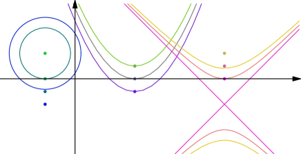
Figure 7: Different $\sigma$-implementations of the same $\breve{\sigma}$-zero-radius cycles and corresponding foci.

Geometrically $\breve{\sigma}$-zero-radius cycles are $\sigma$-implemented by $Q$ from Defn. 3.1 rather differently, see Fig. 7. Some notable rules are:

• Implementations are zero-radius cycles in the standard sense: the point $ue_{0}-ve_{1}$ in elliptic case and the light cone with the centre at $ue_{0}+ve_{1}$ in hyperbolic space [Cnops02a].

• Implementations are parabolas with focal length $v/2$ and the real axis passing through the $\breve{\sigma}$-focus. In other words, for $\breve{\sigma}=-1$ focus at $(u,v)$ (the real axis is directrix), for $\breve{\sigma}=0$ focus at $(u,v/2)$ (the real axis passes through the vertex), for $\breve{\sigma}=1$ focus at $(u,0)$ (the real axis passes through the focus). Such parabolas as well have “zero-radius” for a suitable parabolic metric, see Lemma 5.7.

• $\sigma$-Implementations are corresponding conic sections which touch the real axis.

Remark 3.14.

The above “touching” property of zero-radius cycles for $\breve{\sigma}=0$ is an example of boundary effect inside the domain mentioned in Rem. 3.6. It is not surprising after all since $SL_{2}{}(\mathbb{R}{})$ action on the upper half-plane may be considered as an extension of its action on the real axis.

$\breve{\sigma}$-Zero-radius cycles are significant since they are completely determined by their centres and thus “encode” points into the “cycle language”. The following result states that this encoding is Möbius invariant as well.

Lemma 3.15.

The conjugate $g^{-1}Z^{s}_{\breve{\sigma}}(y)g$ of a $\breve{\sigma}$-zero-radius cycle $Z^{s}_{\breve{\sigma}}(y)$ with $g\in SL_{2}{}(\mathbb{R}{})$ is a $\breve{\sigma}$-zero-radius cycle $Z^{s}_{\breve{\sigma}}(g\cdot y)$ with centre at $g\cdot y$—the Möbius transform of the centre of $Z^{s}_{\breve{\sigma}}(y)$.

Proof 3.16.

This may be calculated in GiNaC [Kisil05b]*§ LABEL:G-sec:mobi-invar-cycl.

Another important class of cycles is given by next definition based on the invariant inner product (3.7) and the invariance of the real line.

Definition 3.17.

Self-adjoint cycle for $\breve{\sigma}\neq 0$ are defined by the condition $\Re\left\langle{C^{s}_{\breve{\sigma}}},R^{s}_{\breve{\sigma}}\right\rangle=0$, where $R^{s}_{\breve{\sigma}}$ corresponds to the “real” axis $v=0$ and $\Re$ denotes the real part of a Clifford number.

Explicitly a self-adjoint cycle ${C^{s}_{\breve{\sigma}}}$ is defined by $n=0$ in (3.1). Geometrically they are:

• circles or hyperbolas with centres on the real line;

• vertical lines, which are also “parabolic circles” [Yaglom79], i.e. are given by $\left\|x-y\right\|=r^{2}$ in the parabolic metric defined below in (5.3).

Lemma 3.18.

Self-adjoint cycles form a family, which is invariant under the Möbius transformations.

Proof 3.19.

The proof is either geometrically obvious from the transformations described in Section 2.2, or follows analytically from the action described in Proposition 3.3.

Remark 3.20.

Geometric objects, which are invariant under infinitesimal action of $SL_{2}{}(\mathbb{R}{})$, were studied recently in papers [KonovenkoLychagin08a, Konovenko09a].

4 Joint invariants: Orthogonality and Inversions

4.1 Invariant Orthogonality Type Conditions

We already use the matrix invariants of a single cycle in Definition 3.11, 3.13 and 3.17. Now we will consider joint invariants of several cycles. Obviously, the relation $\mathop{tr}({C^{s}_{\breve{\sigma}}}{\tilde{C}^{s}_{\breve{\sigma}}})=0$ between two cycles is invariant under Möbius transforms and characterises the mutual disposition of two cycles ${C^{s}_{\breve{\sigma}}}$ and ${\tilde{C}^{s}_{\breve{\sigma}}}$. More generally the relations

$$\mathop{tr}(p({{C^{s}_{\breve{\sigma}}}}^{(1)},\ldots,{{C^{s}_{\breve{\sigma}}}}^{(n)}))=0\quad\text{or}\quad\det(p({{C^{s}_{\breve{\sigma}}}}^{(1)},\ldots,{{C^{s}_{\breve{\sigma}}}}^{(n)}))=0$$ (4.1)

between $n$ cycles ${{C^{s}_{\breve{\sigma}}}}^{(1)}$, …, ${{C^{s}_{\breve{\sigma}}}}^{(n)}$ based on a polynomial $p(x^{(1)},\ldots,x^{(n)})$ of $n$ non-commuting variables $x^{\prime}$, …, $x^{(n)}$ is Möbius invariant if $p(x^{(1)},\ldots,x^{(n)})$ is homogeneous in every $x^{(i)}$. Non-homogeneous polynomials will also create Möbius invariants if we substitute cycles’ $\det$-normalised matrices only. Let us consider some lower order realisations of (4.1).

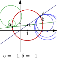
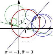
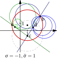
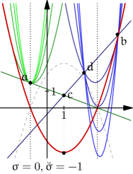
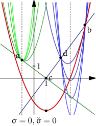
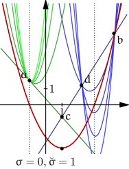
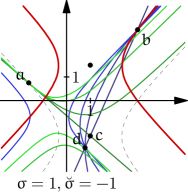
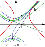
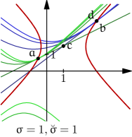
Figure 8: Orthogonality of the first kind in nine combinations.
Each picture presents two groups (green and blue) of cycles which are orthogonal to the red cycle ${C^{s}_{\breve{\sigma}}}$. Point $b$ belongs to ${C^{s}_{\breve{\sigma}}}$ and the family of blue cycles passing through $b$ is orthogonal to ${C^{s}_{\breve{\sigma}}}$. They all also intersect in the point $d$ which is the inverse of $b$ in ${C^{s}_{\breve{\sigma}}}$. Any orthogonality is reduced to the usual orthogonality with a new (“ghost”) cycle (shown by the dashed line), which may or may not coincide with ${C^{s}_{\breve{\sigma}}}$. For any point $a$ on the “ghost” cycle the orthogonality is reduced to the local notion in the terms of tangent lines at the intersection point. Consequently such a point $a$ is always the inverse of itself.

Definition 4.1.

Two cycles ${C^{s}_{\breve{\sigma}}}$ and ${\tilde{C}^{s}_{\breve{\sigma}}}$ are $\breve{\sigma}$-orthogonal if the real part of their inner product (3.7) vanishes:

$$\Re\left\langle{C^{s}_{\breve{\sigma}}},{\tilde{C}^{s}_{\breve{\sigma}}}\right\rangle=0\quad\text{ or, equivalently, }\quad\left\langle{C^{s}_{\breve{\sigma}}},{\tilde{C}^{s}_{\breve{\sigma}}}\right\rangle+\left\langle{\tilde{C}^{s}_{\breve{\sigma}}},{C^{s}_{\breve{\sigma}}}\right\rangle=0$$ (4.2)

In light of (3.8) the zero-radius cycles (Defn. 3.13) are also called self-orthogonal or isotropic.

Lemma 4.2.

The $\breve{\sigma}$-orthogonality condition (4.2) is invariant under Möbius transformations.

Proof 4.3.

It immediately follows from Definition 4.1, formula (3.4) and the invariance of trace under similarity.

We also get by the straightforward calculation [Kisil05b]*§ LABEL:G-sec:vari-orth-cond:

Lemma 4.4.

The $\breve{\sigma}$-orthogonality (4.2) of cycles ${\tilde{C}^{s}_{\breve{\sigma}}}$ and ${C^{s}_{\breve{\sigma}}}$ is given through their defining equation (3.1) coefficients by

$$2\breve{\sigma}\tilde{n}n-2\tilde{l}l+\tilde{k}m+\tilde{m}k=0.$$ (a)

or specifically by

$$-2\tilde{n}n-2\tilde{l}l+\tilde{k}m+\tilde{m}k = 0,$$ (e)

$$-2\tilde{l}l+\tilde{k}m+\tilde{m}k = 0,$$ (p)

$$2\tilde{n}n-2\tilde{l}l+\tilde{k}m+\tilde{m}k = 0$$ (h)

in the elliptic, parabolic and hyperbolic cases of ${\mathcal{C}\kern-1.19995pt\ell(\sigma)}$ correspondingly.

Note that the orthogonality identity (a) is linear for coefficients of one cycle if the other cycle is fixed. Thus we obtain several simple conclusions.

Corollary 4.5.

1. A $\breve{\sigma}$-self-orthogonal cycle is $\breve{\sigma}$-zero-radius one (3.11).

2. For $\breve{\sigma}=\pm 1$ there is no non-trivial cycle orthogonal to all other non-trivial cycles.
   For $\breve{\sigma}=0$ only the real axis $v=0$ is orthogonal to all other non-trivial cycles.

3. For $\breve{\sigma}=\pm 1$ any cycle is uniquely defined by the family of cycles orthogonal to it, i.e. $({C^{s}_{\breve{\sigma}}}^{\perp})^{\perp}=\{{C^{s}_{\breve{\sigma}}}\}$ .
   For $\breve{\sigma}=0$ the set $({C^{s}_{\breve{\sigma}}}^{\perp})^{\perp}$ consists of all cycles which have the same roots as ${C^{s}_{\breve{\sigma}}}$, see middle column of pictures in Fig. 8.

We can visualise the orthogonality with a zero-radius cycle as follow:

Lemma 4.6.

A cycle ${C^{s}_{\breve{\sigma}}}$ is $\breve{\sigma}$-orthogonal to $\sigma$-zero-radius cycle $Z^{s}_{\sigma}(u,v)$ if

$$k(u^{2}k-\sigma v^{2})-2\left\langle(l,n),(u,\breve{\sigma}v)\right\rangle+m=0,$$ (4.4)

i.e. $\sigma$-implementation of ${C^{s}_{\breve{\sigma}}}$ is passing through the point $(u,\breve{\sigma}v)$, which $\breve{\sigma}$-centre of $Z^{s}_{\sigma}(u,v)$.

The important consequence of the above observations is the possibility to extrapolate results from zero-radius cycles to the entire space.

Proposition 4.7.

Let $T:\mathbb{P}^{3}{}\rightarrow\mathbb{P}^{3}{}$ is an orthogonality preserving map of the cycles space, i.e. $\left\langle{C^{s}_{\breve{\sigma}}},{\tilde{C}^{s}_{\breve{\sigma}}}\right\rangle=0\ \Leftrightarrow\left\langle T{C^{s}_{\breve{\sigma}}},T{\tilde{C}^{s}_{\breve{\sigma}}}\right\rangle=0$. Then for $\sigma\neq 0$ there is a map $T_{\sigma}:\mathbb{R}^{\sigma}{}\rightarrow\mathbb{R}^{\sigma}{}$, such that $Q$ intertwines $T$ and $T_{\sigma}$:

$$QT_{\sigma}=TQ.$$ (4.5)

Proof 4.8.

If $T$ preserves the orthogonality (i.e. the inner product (3.7) and consequently the determinant from (3.8)) then by the image $TZ^{s}_{\breve{\sigma}}(u,v)$ of a zero-radius cycle $Z^{s}_{\breve{\sigma}}(u,v)$ is again a zero-radius cycle $Z^{s}_{\breve{\sigma}}(u_{1},v_{1})$ and we can define $T_{\sigma}$ by the identity $T_{\sigma}:(u,v)\mapsto(u_{1},v_{1})$.

To prove the intertwining property (4.5) we need to show that if a cycle ${C^{s}_{\breve{\sigma}}}$ passes through $(u,v)$ then the image $T{C^{s}_{\breve{\sigma}}}$ passes through $T_{\sigma}(u,v)$. However for $\sigma\neq 0$ this is a consequence of the $T$-invariance of orthogonality and the expression of the point-to-cycle incidence through the orthogonality from Lemma 4.6.

Corollary 4.9.

Let $T_{i}:\mathbb{P}^{3}{}\rightarrow\mathbb{P}^{3}{}$, $i=1,2$ are two orthogonality preserving maps of the cycles space. If they coincide on the subspace of $\breve{\sigma}$-zero-radius cycles, $\breve{\sigma}\neq 0$, then they are identical in the whole $\mathbb{P}^{3}{}$.

Remark 4.10.

Note, that the orthogonality is reduced to local notion in terms of tangent lines to cycles in their intersection points only for $\sigma\breve{\sigma}=1$, i.e. this happens only in NW and SE corners of Fig. 8. In other cases the local condition can be formulated in term of “ghost” cycle defined below.

We denote by $\chi(\sigma)$ the Heaviside function:

$$\chi(t)=\left\{\begin{array}[]{ll}1,&t\geq 0;\\ -1,&t<0.\end{array}\right.$$ (4.6)

Proposition 4.11.

Let cycles ${C_{\breve{\sigma}}}$ and ${\tilde{C}_{\breve{\sigma}}}$ be $\breve{\sigma}$-orthogonal. For their $\sigma$-implementations we define the ghost cycle ${\hat{C}_{\breve{\sigma}}}$ by the following two conditions:

1. $\chi(\sigma)$-centre of ${\hat{C}_{\breve{\sigma}}}$ coincides with $\breve{\sigma}$-centre of ${C_{\breve{\sigma}}}$.

2. Determinant of ${\hat{C}^{1}_{\sigma}}$ is equal to determinant of ${C^{\chi(\breve{\sigma})}_{\sigma}}$.

Then:

1. ${\hat{C}_{\sigma}}$ coincides with ${C_{\sigma}}$ if $\sigma\breve{\sigma}=1$;

2. ${\hat{C}_{\sigma}}$ has common roots (real or imaginary) with ${C_{\sigma}}$;

3. In the $\sigma$-implementation the tangent line to ${\tilde{C}_{\breve{\sigma}}}$ at points of its intersections with the ghost cycle ${\hat{C}_{\sigma}}$ are passing the $\sigma$-centre of ${\hat{C}_{\sigma}}$.

Proof 4.12.

The calculations are done in GiNaC, see [Kisil05b]*§ LABEL:G-sec:ghost-cycle. For illustration see Fig. 8, where the ghost cycle is shown by the black dashed line.

Consideration of the ghost cycle does present the orthogonality in the local terms however it hides the symmetry of this relation.

Remark 4.13.

Elliptic and hyperbolic ghost cycles are symmetric in the real line, the parabolic ghost cycle has its centre on it, see Fig. 8. This is an illustration to the boundary effect from Rem. 3.6.

4.2 Inversions in Cycles

Definition 3.1 associates a $2\times 2$-matrix to any cycle. Similarly to $SL_{2}{}(\mathbb{R}{})$ action (2.3) we can consider a fraction-linear transformation on $\mathbb{R}^{\sigma}{}$ defined by such a matrix:

$${C^{s}_{\sigma}}:ue_{0}+ve_{1}\mapsto{C^{s}_{\sigma}}(ue_{0}+ve_{1})=\frac{(le_{0}+ne_{1})(ue_{0}+ve_{1})+m}{k(ue_{0}+ve_{1})-(le_{0}+ne_{1})}$$ (4.7)

where ${C^{s}_{\sigma}}$ is as usual (3.2)

$${C^{s}_{\sigma}}=\begin{pmatrix}le_{0}+ne_{1}&m\\ k&-le_{0}-ne_{1}\end{pmatrix}.$$

Another natural action of cycles in the matrix form is given by the conjugation on other cycles:

$${C^{s}_{\breve{\sigma}}}:{\tilde{C}^{s}_{\breve{\sigma}}}\mapsto{C^{s}_{\breve{\sigma}}}{\tilde{C}^{s}_{\breve{\sigma}}}{C^{s}_{\breve{\sigma}}}.$$ (4.8)

Note that ${C^{s}_{\breve{\sigma}}}{C^{s}_{\breve{\sigma}}}=-\det({C^{s}_{\breve{\sigma}}})I$, where $I$ is the identity matrix. Thus the definition (4.8) is equivalent to expressions ${C^{s}_{\breve{\sigma}}}{\tilde{C}^{s}_{\breve{\sigma}}}{C^{s}_{\breve{\sigma}}}^{-1}$ for $\det{C^{s}_{\breve{\sigma}}}\neq 0$ since cycles form a projective space. There is a connection between two actions (4.7) and (4.8) of cycles, which is similar to $SL_{2}{}(\mathbb{R}{})$ action in Lemma 3.15.

Lemma 4.14.

Let $\det{C^{s}_{\breve{\sigma}}}\neq 0$, then:

1. The conjugation (4.8) preserves the orthogonality relation (4.2).

2. The image ${C^{s_{2}}_{\sigma}}\tilde{Z}^{s_{1}}_{\sigma}(u,v){C^{s_{2}}_{\sigma}}$ of a $\sigma$-zero-radius cycle $\tilde{Z}^{s_{1}}_{\sigma}$ under the conjugation (4.8) is a $\sigma$-zero-radius cycle $\tilde{Z}^{s_{1}}_{\sigma}(u^{\prime},v^{\prime})$, where $(u^{\prime},v^{\prime})$ is calculated by the linear-fractional transformation (4.7) $(u^{\prime},v^{\prime})={C^{s_{1}s_{2}}_{\sigma}}(u,v)$ associated to the cycle ${C^{s_{1}s_{2}}_{\sigma}}$.

3. Both formulae (4.7) and (4.8) define the same transformation of the point space.

Proof 4.15.

The first part is obvious, the second is calculated in GiNaC [Kisil05b]*§ LABEL:G-sec:cycles-conjugation. The last part follows from the first two and Prop. 4.7.

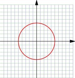
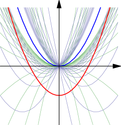
(a)  (b)
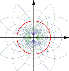
(c)  (d)

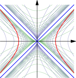
Figure 9: Three types of inversions of the rectangular grid. The initial rectangular grid (a) is inverted elliptically in the unit circle (shown in red) on (b), parabolically on (c) and hyperbolically on (d). The blue cycle (collapsed to a point at the origin on (b)) represent the image of the cycle at infinity under inversion.

There are at least two natural ways to define inversions in cycles. One of them use the orthogonality condition, another define them as “reflections in cycles”.

Definition 4.16.

1. Inversion in a cycle ${C^{s}_{\sigma}}$ sends a point $p$ to the second point $p^{\prime}$ of intersection of all cycles orthogonal to ${C^{s}_{\sigma}}$ and passing through $p$.

2. Reflection in a cycle ${C^{s}_{\sigma}}$ is given by $M^{-1}RM$ where $M$ sends the cycle ${C^{s}_{\sigma}}$ into the horizontal axis and $R$ is the mirror reflection in that axis.

We are going to see that inversions are given by (4.7) and reflections are expressed through (4.8), thus they are essentially the same in light of Lemma 4.14.

Remark 4.17.

Here is a simple example where usage of complex (dual or double) numbers is weaker then Clifford algebras, see Rem. 2.1. A reflection of a cycle in the axis $v=0$ is represented by the conjugation (4.8) with the corresponding matrix $\begin{pmatrix}\breve{e}_{1}&0\\ 0&-\breve{e}_{1}\end{pmatrix}$. The same transformation in term of complex numbers should involve a complex conjugation and thus cannot be expressed by multiplication.

Since we have three different EPH orthogonality between cycles there are also three different inversions:

Proposition 4.18.

A cycle ${\tilde{C}^{s}_{\breve{\sigma}}}$ is orthogonal to a cycle ${C^{s}_{\breve{\sigma}}}$ if for any point $u_{1}e_{0}+v_{1}e_{1}\in{\tilde{C}^{s}_{\breve{\sigma}}}$ the cycle ${\tilde{C}^{s}_{\breve{\sigma}}}$ is also passing through its image

$$u_{2}e_{0}+v_{2}e_{1}=\begin{pmatrix}le_{0}+sre_{1}&m\\ k&le_{0}+sre_{1}\end{pmatrix}(u_{1}e_{0}+v_{1}e_{1})$$ (4.9)

under the Möbius transform defined by the matrix ${C^{s}_{\breve{\sigma}}}$. Thus the point $u_{2}e_{0}+v_{2}e_{1}={C^{s}_{\breve{\sigma}}}(u_{1}e_{0}+v_{1}e_{1})$ is the inversion of $u_{1}e_{0}+v_{1}e_{1}$ in ${C^{s}_{\breve{\sigma}}}$.

Proof 4.19.

The symbolic calculations done by GiNaC[Kisil05b]*§ LABEL:G-sec:orth-invers.

Proposition 4.20.

The reflection 4.16.2 of a zero-radius cycle $Z^{s}_{\breve{\sigma}}$ in a cycle ${C^{s}_{\breve{\sigma}}}$ is given by the conjugation: ${C^{s}_{\breve{\sigma}}}Z^{s}_{\breve{\sigma}}{C^{s}_{\breve{\sigma}}}$.

Proof 4.21.

Let ${\tilde{C}^{s}_{\breve{\sigma}}}$ has the property ${\tilde{C}^{s}_{\breve{\sigma}}}{C^{s}_{\breve{\sigma}}}{\tilde{C}^{s}_{\breve{\sigma}}}=\mathbb{R}{}$. Then ${\tilde{C}^{s}_{\breve{\sigma}}}\mathbb{R}{}{\tilde{C}^{s}_{\breve{\sigma}}}={C^{s}_{\breve{\sigma}}}$. Mirror reflection in the real line is given by the conjugation with $\mathbb{R}{}$, thus the transformation described in 4.16.2 is a conjugation with the cycle ${\tilde{C}^{s}_{\breve{\sigma}}}\mathbb{R}{}{\tilde{C}^{s}_{\breve{\sigma}}}={C^{s}_{\breve{\sigma}}}$ and thus coincide with (4.9).

The cycle ${\tilde{C}^{s}_{\breve{\sigma}}}$ from the above proof can be characterised as follows.

Lemma 4.22.

Let ${C^{s}_{\breve{\sigma}}}=(k,l,n,m)$ be a cycle and for $\breve{\sigma}\neq 0$ the ${\tilde{C}^{s}_{\breve{\sigma}}}$ be given by $(k,l,n\pm\sqrt{\det{C^{\sigma}_{\breve{\sigma}}}},m)$. Then

1. ${\tilde{C}^{s}_{\breve{\sigma}}}{C^{s}_{\breve{\sigma}}}{\tilde{C}^{s}_{\breve{\sigma}}}=\mathbb{R}{}$ and ${\tilde{C}^{s}_{\breve{\sigma}}}\mathbb{R}{}{\tilde{C}^{s}_{\breve{\sigma}}}={C^{s}_{\breve{\sigma}}}$

2. ${\tilde{C}^{s}_{\breve{\sigma}}}$ and ${C^{s}_{\breve{\sigma}}}$ have common roots.

3. In the $\breve{\sigma}$-implementation the cycle ${C^{s}_{\breve{\sigma}}}$ passes the centre of ${\tilde{C}^{s}_{\breve{\sigma}}}$.

Proof 4.23.

This is calculated by GiNaC [Kisil05b]*§ LABEL:G-sec:reflection-cycles. Also one can direct observe 4.22.2 for real roots, since they are fixed points of the inversion. Also the transformation of ${C^{s}_{\breve{\sigma}}}$ to a flat cycle implies that ${C^{s}_{\breve{\sigma}}}$ is passing the centre of inversion, hence 4.22.3.

In [Yaglom79]*§ 10 the inversion of second kind related to a parabola $v=k(u-l)^{2}+m$ was defined by the map:

$$(u,v)\mapsto(u,2(k(u-l)^{2}+m)-v),$$ (4.10)

i.e. the parabola bisects the vertical line joining a point and its image. Here is the result expression this transformation through the usual inversion in parabolas:

Proposition 4.24.

The inversion of second kind (4.10) is a composition of three inversions: in parabolas $u^{2}-2lu-4mv-m/k=0$, $u^{2}-2lu-m/k=0$, and the real line.

Proof 4.25.

See symbolic calculation in [Kisil05b]*§ LABEL:G-sec:invers-second-kind.

Remark 4.26.

Yaglom in [Yaglom79]*§ 10 considers the usual inversion (“of the first kind”) only in degenerated parabolas (“parabolic circles”) of the form $u^{2}-2lu+m=0$. However the inversion of the second kind requires for its decomposition like in Prop. 4.24 at least one inversion in a proper parabolic cycle $u^{2}-2lu-2nv+m=0$. Thus such inversions are indeed of another kind within Yaglom’s framework [Yaglom79], but are not in our.

Another important difference between inversions from [Yaglom79] and our wider set of transformations (4.7) is what “special” (vertical) lines does not form an invariant set, as can be seen from Fig. 9(c), and thus they are not “special” lines anymore.

4.3 Focal Orthogonality

It is natural to consider invariants of higher orders which are generated by (4.1). Such invariants shall have at least one of the following properties

• contains a non-linear power of the same cycle;

• accommodate more than two cycles.

The consideration of higher order invariants is similar to a transition from Riemannian geometry to Finsler one [Chern96a, Garasko09a, Pavlov06a].

It is interesting that higher order invariants

1. can be built on top of the already defined ones;

2. can produce lower order invariants.

For each of the two above transitions we consider an example. We already know that a similarity of a cycle with another cycle is a new cycle (4.8). The inner product of later with a third given cycle form a joint invariant of those three cycles:

$$\left\langle{C^{s}_{\breve{\sigma}}}_{1}{C^{s}_{\breve{\sigma}}}_{2}{C^{s}_{\breve{\sigma}}}_{1},{C^{s}_{\breve{\sigma}}}_{3}\right\rangle,$$ (4.11)

which is build from the second-order invariant $\left\langle\cdot,\cdot\right\rangle$. Now we can reduce the order of this invariant by fixing ${C^{s}_{\breve{\sigma}}}_{3}$ be the real line (which is itself invariant). The obtained invariant of two cycles deserves a special consideration. Alternatively it emerges from Definitions 4.1 and 3.17.

Definition 4.27.

The focal orthogonality (f-orthogonality) of a cycle ${C^{s}_{\breve{\sigma}}}$ to a cycle ${\tilde{C}^{s}_{\breve{\sigma}}}$ is defined by the condition that the cycle ${C^{s}_{\breve{\sigma}}}{\tilde{C}^{s}_{\breve{\sigma}}}{C^{s}_{\breve{\sigma}}}$ is orthogonal (in the sense of Definition 4.1) to the real line, i.e is a self-adjoint cycle in the sense of Definition 3.17. Analytically this is defined by

$$\Re\mathop{tr}({C^{s}_{\breve{\sigma}}}{\tilde{C}^{s}_{\breve{\sigma}}}{C^{s}_{\breve{\sigma}}}R^{s}_{\breve{\sigma}})=0$$ (4.12)

and we denote it by ${C^{s}_{\breve{\sigma}}}\dashv{\tilde{C}^{s}_{\breve{\sigma}}}$.

Remark 4.28.

This definition is explicitly based on the invariance of the real line and is an illustration to the boundary value effect from Rem. 3.6.

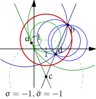
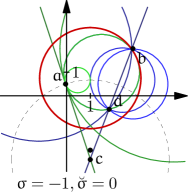
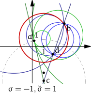
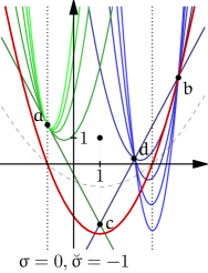
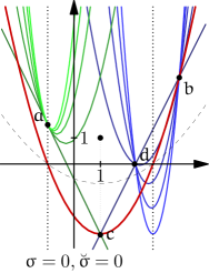
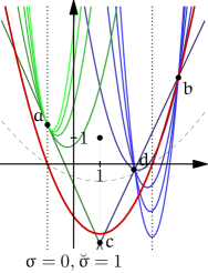
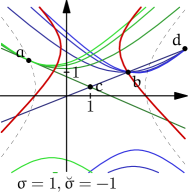
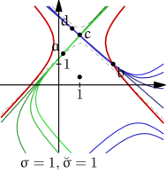
Figure 10: Focal orthogonality in all nine combinations. To highlight both similarities and distinctions with the ordinary orthogonality we use the same notations as that in Fig. 8. The cycles ${\tilde{C}^{\breve{\sigma}}_{\breve{\sigma}}}$ from Proposition 4.33 are drawn by dashed lines.

Remark 4.29.

It is easy to observe the following

1. f-orthogonality is not a symmetric: ${C^{s}_{\breve{\sigma}}}\dashv{\tilde{C}^{s}_{\breve{\sigma}}}$ does not implies ${\tilde{C}^{s}_{\breve{\sigma}}}\dashv{C^{s}_{\breve{\sigma}}}$;

2. Since the real axis $\mathbb{R}{}$ and orthogonality (4.2) are $SL_{2}{}(\mathbb{R}{})$-invariant objects f-orthogonality is also $SL_{2}{}(\mathbb{R}{})$-invariant.

However an invariance of f-orthogonality under inversion of cycles required some study since the real line is not an invariant of such transformations in general.

Lemma 4.30.

The image ${C^{s_{1}}_{\breve{\sigma}}}R^{s}_{\breve{\sigma}}{C^{s_{1}}_{\breve{\sigma}}}$ of the real line under inversion in ${C^{s_{1}}_{\breve{\sigma}}}=(k,l,n,m)$ is the cycle:

$$(2ss_{1}\breve{\sigma}kn,\ 2ss_{1}\breve{\sigma}ln,\ s^{2}(l^{2}+\breve{\sigma}n^{2}-mk),\ 2ss_{1}\breve{\sigma}mn).$$

It is the real line if $s\cdot\det({C^{s_{1}}_{\breve{\sigma}}})\neq 0$ and either

1. $s_{1}n=0$, in this case it is a composition of $SL_{2}{}(\mathbb{R}{})$-action by $\begin{pmatrix}l&-me_{0}\\ ke_{0}&-l\end{pmatrix}$ and the reflection in the real line; or

2. $\breve{\sigma}=0$, i.e. the parabolic case of the cycle space.

If this condition is satisfied than f-orthogonality preserved by the inversion ${\tilde{C}^{s}_{\breve{\sigma}}}\rightarrow{C^{s_{1}}_{\breve{\sigma}}}{\tilde{C}^{s}_{\breve{\sigma}}}{C^{s_{1}}_{\breve{\sigma}}}$ in ${\tilde{C}^{s}_{\breve{\sigma}}}$.

The following explicit expressions of f-orthogonality reveal further connections with cycles’ invariants.

Proposition 4.31.

f-orthogonality of ${{C^{s}_{p}}}$ to ${{\tilde{C}^{s}_{p}}}$ is given by either of the following equivalent identities

$$\tilde{n}(l^{2}-\breve{e}_{1}^{2}n^{2}-mk)+\tilde{m}nk-2\tilde{l}nl+\tilde{k}mn = 0,\qquad\textrm{ or}$$

$$\tilde{n}\det({C^{s}_{\breve{\sigma}}})+n\left\langle{C^{s}_{p}},{\tilde{C}^{s}_{p}}\right\rangle = 0.$$

Proof 4.32.

This is another GiNaC calculation [Kisil05b]*§ LABEL:G-sec:expr-orth-s.k

The f-orthogonality may be again related to the usual orthogonality through an appropriately chosen f-ghost cycle, compare the next Proposition with Prop. 4.11:

Proposition 4.33.

Let ${C^{s}_{\breve{\sigma}}}$ be a cycle, then its f-ghost cycle ${\tilde{C}^{\breve{\sigma}}_{\breve{\sigma}}}={C^{\chi(\sigma)}_{\breve{\sigma}}}\mathbb{R}^{\breve{\sigma}}_{\breve{\sigma}}{}{C^{\chi(\sigma)}_{\breve{\sigma}}}$ is the reflection of the real line in ${C^{\chi(\sigma)}_{\breve{\sigma}}}$, where $\chi(\sigma)$ is the Heaviside function 4.6. Then

1. Cycles ${C^{s}_{\breve{\sigma}}}$ and ${\tilde{C}^{\breve{\sigma}}_{\breve{\sigma}}}$ have the same roots.

2. $\chi(\sigma)$-Centre of ${\tilde{C}^{\breve{\sigma}}_{\breve{\sigma}}}$ coincides with the $\breve{\sigma}$-focus of ${C^{s}_{\breve{\sigma}}}$, consequently all lines f-orthogonal to ${C^{s}_{\breve{\sigma}}}$ are passing one of its foci.

3. s-Reflection in ${C^{s}_{\breve{\sigma}}}$ defined from f-orthogonality (see Definition 4.16.1) coincides with usual inversion in ${\tilde{C}^{\breve{\sigma}}_{\breve{\sigma}}}$.

Proof 4.34.

This again is calculated in GiNaC, see [Kisil05b]*§ LABEL:G-sec:invers-from-orth.

For the reason 4.33.2 this relation between cycles may be labelled as focal orthogonality, cf. with 4.11.1. It can generates the corresponding inversion similar to Defn. 4.16.1 which obviously reduces to the usual inversion in the f-ghost cycle. The extravagant f-orthogonality will unexpectedly appear again from consideration of length and distances in the next section and is useful for infinitesimal cycles § 6.1.

5 Metric Properties from Cycle Invariants

So far we discussed only invariants like orthogonality, which are related to angles. Now we turn to metric properties similar to distance.

5.1 Distances and Lengths

The covariance of cycles (see Lemma 2.14) suggests them as “circles” in each of the EPH cases. Thus we play the standard mathematical game: turn some properties of classical objects into definitions of new ones.

Definition 5.1.

The $\breve{\sigma}$-radius of a cycle ${C^{s}_{\breve{\sigma}}}$ if squared is equal to the $\breve{\sigma}$-determinant of cycle’s $k$-normalised (see Defn. 3.10) matrix, i.e.

$$r^{2}=\frac{\det{C^{s}_{\breve{\sigma}}}}{k^{2}}=\frac{l^{2}-\breve{\sigma}n^{2}-km}{k^{2}}.$$ (5.1)

As usual, the $\breve{\sigma}$-diameter of a cycles is two times its radius.

Lemma 5.2.

The $\breve{\sigma}$-radius of a cycle ${C^{s}_{\breve{\sigma}}}$ is equal to $1/k$, where $k$ is $(2,1)$-entry of $\det$-normalised matrix (see Defn. 3.10) of the cycle.

Geometrically in various EPH cases this corresponds to the following

1. The value of (5.1) is the usual radius of a circle or hyperbola;

2. The diameter of a parabola is the (Euclidean) distance between its (real) roots, i.e. solutions of $ku^{2}-2lu+m=0$, or roots of its “adjoint” parabola $-ku^{2}+2lu+m-\frac{2l^{2}}{k}=0$ (see Fig. 11(a)).

Remark 5.3.

Note that

$$r^{2}_{\breve{\sigma}}=-4*f*u_{\breve{\sigma}},$$

where $r^{2}_{\breve{\sigma}}$ is the square of cycle’s $\breve{\sigma}$-radius, $u_{\breve{\sigma}}$ is the second coordinate of its $\breve{\sigma}$-focus and $f$ its focal length.

(a) (b)

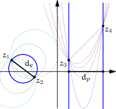
Figure 11: (a) The square of the parabolic diameter is the square of the distance between roots if they are real ($z_{1}$ and $z_{2}$), otherwise the negative square of the distance between the adjoint roots ($z_{3}$ and $z_{4}$).
(b) Distance as extremum of diameters in elliptic ($z_{1}$ and $z_{2}$) and parabolic ($z_{3}$ and $z_{4}$) cases.

An intuitive notion of a distance in both mathematics and the everyday life is usually of a variational nature. We natural perceive the shortest distance between two points delivered by the straight lines and only then can define it for curves through an approximation. This variational nature echoes also in the following definition.

Definition 5.4.

The $(\sigma,\breve{\sigma})$-distance between two points is the extremum of $\breve{\sigma}$-diameters for all $\sigma$-cycles passing through both points.

During geometry classes we oftenly make measurements with a compass, which is based on the idea that a cycle is locus of points equidistant from its centre. We can expand it for all cycles in the following definition:

Definition 5.5.

The $\breve{\sigma}$-length from a $\mathring{\sigma}$-centre or from a $\mathring{\sigma}$-focus of a directed interval $\overrightarrow{AB}$ is the $\breve{\sigma}$-radius of the $\sigma$-cycle with its $\mathring{\sigma}$-centre or $\mathring{\sigma}$-focus correspondingly at the point $A$ which passes through $B$. These lengths are denoted by $l_{c}(\overrightarrow{AB})$ and $l_{f}(\overrightarrow{AB})$ correspondingly.

Remark 5.6.

1. Note that the distance is a symmetric functions of two points by its definition and this is not necessarily true for lengths. For modal logic of non-symmetric distances see, for example, [KuruczWolterZakharyaschev05]. However the first axiom ($l(x,y)=0$ iff $x=y$) should be modified as follows:

   $$(l(x,y)=0\text{ and }l(x,y)=0)\text{ iff }x=y.$$

2. A cycle is uniquely defined by elliptic or hyperbolic centre and a point which it passes. However the parabolic centre is not so useful. Correspondingly $(\sigma,0)$-length from parabolic centre is not properly defined.

Lemma 5.7.

1. The cycle of the form (3.11) has zero radius.

2. The distance between two points $y=e_{0}u+e_{1}v$ and $y^{\prime}=e_{0}u^{\prime}+e_{1}v^{\prime}$ in the elliptic or hyperbolic spaces is

   $$d^{2}(y,y^{\prime})=\frac{\breve{\sigma}((u-u^{\prime})^{2}-\sigma(v-v^{\prime})^{2})+4(1-\sigma\breve{\sigma})vv^{\prime}}{(u-u^{\prime})^{2}\breve{\sigma}-(v-v^{\prime})^{2}}((u-u^{\prime})^{2}-\sigma(v-v^{\prime})^{2}),$$ (5.2)

   and in parabolic case it is (see Fig. 11(b) and [Yaglom79]*p. 38, (5))

   $$d^{2}(y,y^{\prime})=(u-u^{\prime})^{2}.$$ (5.3)

Proof 5.8.

Let ${C^{\sigma}_{s}}(l)$ be the family of cycles passing through both points $(u,v)$ and $(u^{\prime},v^{\prime})$ (under the assumption $v\neq v^{\prime}$) and parametrised by its coefficient $l$ in the defining equation (2.10). By a calculation done in GiNaC [Kisil05b]*§ LABEL:G-sec:dist-betw-points we found that the only critical point of $\det({C^{\sigma}_{s}}(l))$ is:

$$l_{0}=\frac{1}{2}\left((u^{\prime}+u)+(\breve{\sigma}\sigma-1)\frac{(u^{\prime}-u)(v^{2}-v^{\prime 2})}{(u^{\prime}-u)^{2}\breve{\sigma}-(v-v^{\prime})^{2}}\right),$$ (5.4)

[Note that in the case $\sigma\breve{\sigma}=1$, i.e. both points and cycles spaces are simultaneously either elliptic or hyperbolic, this expression reduces to the expected midpoint $l_{0}=\frac{1}{2}(u+u^{\prime})$.] Since in the elliptic or hyperbolic case the parameter $l$ can take any real value, the extremum of $\det({C^{\sigma}_{s}}(l))$ is reached in $l_{0}$ and is equal to (5.2) (calculated by GiNaC [Kisil05b]*§ LABEL:G-sec:dist-betw-points). A separate calculation for the case $v=v^{\prime}$ gives the same answer.

In the parabolic case the possible values of $l$ are either in $(-\infty,\frac{1}{2}(u+u^{\prime}))$, or $(\frac{1}{2}(u+u^{\prime}),\infty)$, or the only value is $l=\frac{1}{2}(u+u^{\prime})$ since for that value a parabola should flip between upward and downward directions of its branches. In any of those cases the extremum value corresponds to the boundary point $l=\frac{1}{2}(u+u^{\prime})$ and is equal to (5.3).

Corollary 5.9.

If cycles ${C^{s}_{\breve{\sigma}}}$ and ${\tilde{C}^{s}_{\breve{\sigma}}}$ are normalised by conditions $k=1$ and $\tilde{k}=1$ then

$$\left\langle{C^{s}_{\breve{\sigma}}},{\tilde{C}^{s}_{\breve{\sigma}}}\right\rangle=\left|c-\tilde{c}\right|_{\breve{\sigma}}^{2}-r_{\breve{\sigma}}^{2}-\tilde{r}_{\breve{\sigma}}^{2},$$

where $\left|c-c\right|_{\breve{\sigma}}^{2}=(l-\tilde{l})^{2}-\breve{\sigma}(n-\tilde{n})^{2}$ is the square of $\breve{\sigma}$-distance between cycles’ centres, $r_{\breve{\sigma}}$ and $\tilde{r}_{\breve{\sigma}}$ are $bs$-radii of the respective cycles.

To get feeling of the identity (5.2) we may observe, that:

$$d^{2}(y,y^{\prime}) = (u-u^{\prime})^{2}+(v-v^{\prime})^{2},\qquad\textrm{ for elliptic values }\sigma=\breve{\sigma}=-1;$$

$$d^{2}(y,y^{\prime}) = (u-u^{\prime})^{2}-(v-v^{\prime})^{2},\qquad\textrm{ for hyperbolic values }\sigma=\breve{\sigma}=1;$$

i.e. these are familiar expressions for the elliptic and hyperbolic spaces. However four other cases ($\sigma\breve{\sigma}=-1$ or $0$) gives quite different results. For example, $d^{2}(y,y^{\prime})\not\rightarrow 0$ if $y$ tense to $y^{\prime}$ in the usual sense.

Remark 5.10.

1. In the three cases $\sigma=\breve{\sigma}=-1$, $0$ or $1$, which were typically studied before, the above distances are conveniently defined through the Clifford algebra multiplications

   $$d_{e,p,h}^{2}(ue_{0}+ve_{1})=-(ue_{0}+ve_{1})^{2}.$$

2. Unless $\sigma=\breve{\sigma}$ the parabolic distance (5.3) is not received from (5.2) by the substitution $\sigma=0$.

Now we turn to calculations of the lengths.

Lemma 5.11.

1. The $\breve{\sigma}$-length from the $\mathring{\sigma}$-centre between two points $y=e_{0}u+e_{1}v$ and $y^{\prime}=e_{0}u^{\prime}+e_{1}v^{\prime}$ is

   $$l_{c_{\breve{\sigma}}}^{2}(y,y^{\prime})=(u-u^{\prime})^{2}-\sigma v^{\prime 2}+2\mathring{\sigma}vv^{\prime}-\breve{\sigma}v^{2}.$$ (5.5)

2. The $\breve{\sigma}$-length from the $\mathring{\sigma}$-focus between two points $y=e_{0}u+e_{1}v$ and $y^{\prime}=e_{0}u^{\prime}+e_{1}v^{\prime}$ is

   $$l_{f_{\breve{\sigma}}}^{2}(y,y^{\prime})=(\mathring{\sigma}-\breve{\sigma})p^{2}-2vp,$$ (5.6)

   where:

   $$p = \mathring{\sigma}\left(-(v^{\prime}-v)\pm\sqrt{\mathring{\sigma}(u^{\prime}-u)^{2}+(v^{\prime}-v)^{2}-\sigma\mathring{\sigma}v^{\prime 2}}\right),\quad\text{if }\mathring{\sigma}\neq 0;$$ (5.7)

   $$p = \frac{(u^{\prime}-u)^{2}-\sigma v^{\prime 2}}{2(v^{\prime}-v)},\quad\text{if }\mathring{\sigma}=0.$$ (5.8)

Proof 5.12.

Identity (5.5) is verified in GiNaC [Kisil05b]*§ LABEL:G-sec:length-direct-interv. For the second part we observe that the parabola with the focus $(u,v)$ passing through $(u^{\prime},v^{\prime})$ has the following parameters:

$$k=1,\quad l=u,\quad n=p,\quad m=2\mathring{\sigma}pv^{\prime}-u^{\prime 2}+2uu^{\prime}+\sigma v^{\prime 2}.$$

Then the formula (5.6) is verified by the GiNaC calculation [Kisil05b]*§ LABEL:G-sec:length-interv-from.

Remark 5.13.

1. The value of $p$ in (5.7) is the focal length of either of the two cycles, which are in the parabolic case upward or downward parabolas (corresponding to the plus or minus signs) with focus at $(u,v)$ and passing through $(u^{\prime},v^{\prime})$.

2. In the case $\sigma\breve{\sigma}=1$ the length (5.5) became the standard elliptic or hyperbolic distance $(u-u^{\prime})^{2}-\sigma(v-v^{\prime})^{2}$ obtained in (5.2). Since these expressions appeared both as distances and lengths they are widely used.

   On the other hand in the parabolic space we get three additional lengths besides of distance (5.3):

   $$l_{c_{\breve{\sigma}}}^{2}(y,y^{\prime})=(u-u^{\prime})^{2}+2vv^{\prime}-\breve{\sigma}v^{2}$$

   parametrised by $\breve{\sigma}$ (cf. Remark 1.1.1).

3. The parabolic distance (5.3) can be expressed as

   $$d^{2}(y,y^{\prime})=p^{2}+2(v-v^{\prime})p$$

   in terms of the focal length (5.7), which is an expression similar to (5.6).

5.2 Conformal Properties of Möbius Maps

All lengths $l(\overrightarrow{AB})$ in $\mathbb{R}^{\sigma}{}$ from Definition 5.5 are such that for a fixed point $A$ all level curves of $l(\overrightarrow{AB})=c$ are corresponding cycles: circles, parabolas or hyperbolas, which are covariant objects in the appropriate geometries. Thus we can expect some covariant properties of distances and lengths.

Definition 5.14.

We say that a distance or a length $d$ is $SL_{2}{}(\mathbb{R}{})$-conformal if for fixed $y$, $y^{\prime}\in\mathbb{R}^{\sigma}{}$ the limit:

$$\lim_{t\rightarrow 0}\frac{d(g\cdot y,g\cdot(y+ty^{\prime}))}{d(y,y+ty^{\prime})},\qquad\text{ where }g\in SL_{2}{}(\mathbb{R}{}),$$ (5.9)

exists and its value depends only from $y$ and $g$ and is independent from $y^{\prime}$.

The following proposition shows that $SL_{2}{}(\mathbb{R}{})$-conformality is not rare.

Proposition 5.15.

1. The distance (5.2) is conformal if and only if the type of point and cycle spaces are the same, i.e. $\sigma\breve{\sigma}=1$. The parabolic distance (5.3) is conformal only in the parabolic point space.

2. The lengths from centres (5.5) are conformal for any combination of values of $\sigma$, $\breve{\sigma}$ and $\mathring{\sigma}$.

3. The lengths from foci (5.6) are conformal for $\mathring{\sigma}\neq 0$ and any combination of values of $\sigma$ and $\breve{\sigma}$.

Proof 5.16.

This is another straightforward calculation in GiNaC [Kisil05b]*§ LABEL:G-sec:check-conformity.

The conformal property of the distance (5.2)–(5.3) from Prop. 5.15.1 is well-known, of course, see [Cnops02a, Yaglom79]. However the same property of non-symmetric lengths from Prop. 5.15.2 and 5.15.3 could be hardly expected. The smaller group $SL_{2}{}(\mathbb{R}{})$ (in comparison to all linear-fractional transforms of $\mathbb{R}^{2}{}$) generates bigger number of conformal metrics, cf. Rem. 3.6.

The exception of the case $\mathring{\sigma}=0$ from the conformality in 5.15.3 looks disappointing on the first glance, especially in the light of the parabolic Cayley transform considered later in § 8.2. However a detailed study of algebraic structure invariant under parabolic rotations [Kisil07a] [Kisil09c] removes obscurity from this case. Indeed our Definition 5.14 of conformality heavily depends on the underlying linear structure in $\mathbb{R}^{a}{}$: we measure a distance between points $y$ and $y+ty^{\prime}$ and intuitively expect that it is always small for small $t$. As explained in [Kisil07a]*§ LABEL:W-sec:invar-line-algebra the standard linear structure is incompatible with the parabolic rotations and thus should be replaced by a more relevant one. More precisely, instead of limits $y^{\prime}\rightarrow y$ along the straight lines towards $y$ we need to consider limits along vertical lines, see Fig. 18 and [Kisil07a]*Fig. LABEL:W-fig:p-rotations and Rem. LABEL:W-re:conformality.

Proposition 5.17.

Let the focal length is given by the identity (5.6) with $\sigma=\mathring{\sigma}=0$, e.g.:

$$l_{f_{\breve{\sigma}}}^{2}(y,y^{\prime})=-\breve{\sigma}p^{2}-2vp,\qquad\text{where}\quad p=\frac{(u^{\prime}-u)^{2}}{2(v^{\prime}-v)}$$

Then it is conformal in the sense that for any constant $y=ue_{0}+ve_{1}$ and $y^{\prime}=u^{\prime}e_{0}+v^{\prime}e_{1}$ with a fixed $u^{\prime}$ we have:

$$\lim_{v^{\prime}\rightarrow\infty}\frac{l_{f_{\breve{\sigma}}}(g\cdot y,g\cdot y^{\prime})}{l_{f_{\breve{\sigma}}}(y,y^{\prime})}=\frac{1}{(cu+d)^{2}},\qquad\text{where}\quad g=\begin{pmatrix}a&be_{0}\\ -ce_{0}&d\end{pmatrix}.$$ (5.10)

We also revise the parabolic case of conformality in § 6.2 with a related definition based on infinitesimal cycles.

Remark 5.18.

The expressions of lengths (5.5)–(5.6) are generally non-symmetric and this is a price one should pay for its non-triviality. All symmetric distances lead to nine two-dimensional Cayley-Klein geometries, see [Yaglom79]*App. B [HerranzSantander02a] [HerranzSantander02b]. In the parabolic case a symmetric distance of a vector $(u,v)$ is always a function of $u$ alone, cf. Rem. 5.29. For such a distance a parabolic unit circle consists from two vertical lines (see dotted vertical lines in the second rows on Figs. 8 and 10), which is not aesthetically attractive. On the other hand the parabolic “unit cycles” defined by lengths (5.5) and (5.6) are parabolas, which makes the parabolic Cayley transform (see Section 8.2) very natural.

We can also consider a distance between points in the upper half-plane which is preserved by Möbius transformations, see [Kisil08a].

Lemma 5.19.

Let the line element be $\left|dy\right|^{2}=du^{2}-\sigma dv^{2}$ and the “length of a curve” is given by the corresponding line integral, cf. [Beardon05a]*§ 15.2:

$$\int_{\Gamma}\frac{\left|dy\right|}{v}.$$ (5.11)

Then the length of the curve is preserved under the Möbius transformations.

Proof 5.20.

The proof is based on the following three observations:

1. The line element $\left|dy\right|^{2}=du^{2}-\sigma dv^{2}$ at the point $e_{1}$ is invariant under action of the respective fix-group of this point (see Lem. 2.7).

2. The fraction $\frac{\left|dy\right|}{v}$ is invariant under action of the $ax+b$-group.

3. Möbius action of $SL_{2}{}(\mathbb{R}{})$ in each EPH case is generated by $ax+b$ group and the corresponding fix-subgroup, see Lem. 2.9.

It is known [Beardon05a]*§ 15.2 in the elliptic case that the curve between two points with the shortest length (5.11) is an arc of the circle orthogonal to the real line. Möbius transformations map such arcs to arcs with the same property, therefore the length of such arc calculated in (5.11) is invariant under the Möbius transformations.

Analogously in the hyperbolic case the longest curve between two points is an arc of hyperbola orthogonal to the real line. However in the parabolic case there is no curve delivering the shortest length (5.11), the infimum is $u-u^{\prime}$, see (5.3) and Fig. 11. However we can still define an invariant distance in the parabolic case in the following way:

Lemma 5.21 ([Kisil08a]).

Let two points $w_{1}$ and $w_{2}$ in the upper half-plane are linked by an arc of a parabola with zero $\breve{\sigma}$-radius. Then the length (5.11) along the arc is invariant under Möbius transformations.

5.3 Perpendicularity and Orthogonality

In a Euclidean space the shortest distance from a point to a line is provided by the corresponding perpendicular. Since we have already defined various distances and lengths we may use them for a definition of corresponding notions of perpendicularity.

Definition 5.22.

Let $l$ be a length or distance. We say that a vector $\overrightarrow{AB}$ is $l$-perpendicular to a vector $\overrightarrow{CD}$ if function $l(\overrightarrow{AB}+\varepsilon\overrightarrow{CD})$ of a variable $\varepsilon$ has a local extremum at $\varepsilon=0$. This is denoted by $\overrightarrow{AB}\leftthreetimes\overrightarrow{CD}$.

Remark 5.23.

1. Obviously the $l$-perpendicularity is not a symmetric notion (i.e. $\overrightarrow{AB}\leftthreetimes\overrightarrow{CD}$ does not imply $\overrightarrow{CD}\leftthreetimes\overrightarrow{AB}$) similarly to f-orthogonality, see subsection 4.3.

2. $l$-perpendicularity is obviously linear in $\overrightarrow{CD}$, i.e. $\overrightarrow{AB}\leftthreetimes\overrightarrow{CD}$ implies $\overrightarrow{AB}\leftthreetimes r\overrightarrow{CD}$ for any real non-zero $r$. However $l$-perpendicularity is not generally linear in $\overrightarrow{AB}$, i.e. $\overrightarrow{AB}\leftthreetimes\overrightarrow{CD}$ does not necessarily imply $r\overrightarrow{AB}\leftthreetimes\overrightarrow{CD}$.

There is the following obvious connection between perpendicularity and orthogonality.

Lemma 5.24.

Let $\overrightarrow{AB}$ be $l_{c_{\breve{\sigma}}}$-perpendicular ($l_{f_{\breve{\sigma}}}$-perpendicular) to a vector $\overrightarrow{CD}$. Then the flat cycle (straight line) $AB$, is (s-)orthogonal to the cycle ${C^{s}_{\sigma}}$ with centre (focus) at $A$ passing through $B$. The vector $\overrightarrow{CD}$ is tangent to ${C^{s}_{\sigma}}$ at $B$.

Proof 5.25.

This follows from the relation of centre of (s-)ghost cycle to centre (focus) of (s-)orthogonal cycle stated in Props. 4.11 and 4.33 correspondingly.

Consequently the perpendicularity of vectors $\overrightarrow{AB}$ and $\overrightarrow{CD}$ is reduced to the orthogonality of the corresponding flat cycles only in the cases, when orthogonality itself is reduced to the local notion at the point of cycles intersections (see Rem. 4.10).

Obviously, $l$-perpendicularity turns to be the usual orthogonality in the elliptic case, cf. Lem. 5.28.(e) below. For two other cases the description is given as follows:

Lemma 5.26.

Let $A=(u,v)$ and $B=(u^{\prime},v^{\prime})$. Then

1. $d$-perpendicular (in the sense of (5.2)) to $\overrightarrow{AB}$ in the elliptic or hyperbolic cases is a multiple of the vector

   $$(\sigma(v-v^{\prime})^{3}-(u-u^{\prime})^{2}(v+v^{\prime}(1-2\sigma\breve{\sigma})),\breve{\sigma}(u-u^{\prime})^{3}-(u-u^{\prime})(v-v^{\prime})(-2v^{\prime}+(v+v^{\prime})\breve{\sigma}\sigma)),$$

   which for $\sigma\breve{\sigma}=1$ reduces to the expected value $(v-v^{\prime},\sigma(u-u^{\prime}))$.

2. $d$-perpendicular (in the sense of (5.3)) to $\overrightarrow{AB}$ in the parabolic case is $(0,t)$, $t\in\mathbb{R}{}$ which coincides with the Galilean orthogonality defined in [Yaglom79]*§ 3.

3. $l_{c_{\breve{\sigma}}}$-perpendicular (in the sense of (5.5)) to $\overrightarrow{AB}$ is a multiple of $(\sigma v^{\prime}-\mathring{\sigma}v,u-u^{\prime})$.

4. $l_{f_{\breve{\sigma}}}$-perpendicular (in the sense of (5.6)) to $\overrightarrow{AB}$ is a multiple of $(\sigma v^{\prime}+p,u-u^{\prime})$, where $p$ is defined either by (5.7) or by (5.8) for corresponding values of $\mathring{\sigma}$.

Proof 5.27.

The perpendiculars are calculated by GiNaC [Kisil05b]*§ LABEL:G-sec:calc-perp.

It is worth to have an idea about different types of perpendicularity in the terms of the standard Euclidean geometry. Here are some examples.

Lemma 5.28.

Let $\overrightarrow{AB}=ue_{0}+ve_{1}$ and $\overrightarrow{CD}=u^{\prime}e_{0}+v^{\prime}e_{1}$, then:

1. In the elliptic case the $d$-perpendicularity for $\breve{\sigma}=-1$ means that $\overrightarrow{AB}$ and $\overrightarrow{CD}$ form a right angle, or analytically $uu^{\prime}+vv^{\prime}=0$.

2. In the parabolic case the $l_{f_{\breve{\sigma}}}$-perpendicularity for $\breve{\sigma}=1$ means that $\overrightarrow{AB}$ bisect the angle between $\overrightarrow{CD}$ and the vertical direction or analytically:

   $$u^{\prime}u-v^{\prime}p=u^{\prime}u-v^{\prime}(\sqrt{u^{2}+v^{2}}-v)=0,$$ (5.12)

   where $p$ is the focal length (5.7)

3. In the hyperbolic case the $d$-perpendicularity for $\breve{\sigma}=-1$ means that the angles between $\overrightarrow{AB}$ and $\overrightarrow{CD}$ are bisected by lines parallel to $u=\pm v$, or analytically $u^{\prime}u-v^{\prime}v=0$.

Remark 5.29.

If one attempts to devise a parabolic length as a limit or an intermediate case for the elliptic $l_{e}=u^{2}+v^{2}$ and hyperbolic $l_{p}=u^{2}-v^{2}$ lengths then the only possible guess is $l^{\prime}_{p}=u^{2}$ (5.3), which is too trivial for an interesting geometry.

Similarly the only orthogonality conditions linking the elliptic $u_{1}u_{2}+v_{1}v_{2}=0$ and the hyperbolic $u_{1}u_{2}-v_{1}v_{2}=0$ cases seems to be $u_{1}u_{2}=0$ (see [Yaglom79]*§ 3 and Lem. 5.26.2), which is again too trivial. This support our Remark 1.1.2.

6 Invariants of Infinitesimal Scale

Although parabolic zero-radius cycles defined in 3.13 do not satisfy our expectations for “zero-radius” but they are often technically suitable for the same purposes as elliptic and hyperbolic ones. Yet we may want to find something which fits better for our intuition on “zero sized” object. Here we present an approach based on non-Archimedean (non-standard) analysis [Devis77, Uspenskii88].

6.1 Infinitesimal Radius Cycles

Let $\varepsilon$ be a positive infinitesimal number, i.e. $0<n\varepsilon<1$ for any $n\in\mathbb{N}{}$ [Devis77, Uspenskii88].

Definition 6.1.

A cycle ${C^{s}_{\breve{\sigma}}}$ such that $\det{C^{s}_{\breve{\sigma}}}$ is an infinitesimal number is called infinitesimal radius cycle.

Lemma 6.2.

Let $\breve{\sigma}$ and $\mathring{\sigma}$ be two metric signs and let a point $(u_{0},v_{0})\in\mathbb{R}^{p}{}$ with $v_{0}>0$. Consider a cycle ${C^{s}_{\breve{\sigma}}}$ defined by

$${C^{s}_{\breve{\sigma}}}=(1,u_{0},n,u_{0}^{2}+2nv_{0}-\mathring{\sigma}n^{2}),$$ (6.1)

where

$$n=\left\{\begin{array}[]{ll}\displaystyle\frac{v_{0}-\sqrt{v_{0}^{2}-(\mathring{\sigma}-\breve{\sigma})\varepsilon^{2}}}{\mathring{\sigma}-\breve{\sigma}},&\text{ if }\mathring{\sigma}\neq\breve{\sigma};\\ \displaystyle\frac{\varepsilon^{2}}{2v_{0}},&\text{ if }\mathring{\sigma}=\breve{\sigma}.\end{array}\right.$$ (6.2)

Then

1. The point $(u_{0},v_{0})$ is $\mathring{\sigma}$-focus of the cycle.

2. The square of $\breve{\sigma}$-radius is exactly $-\varepsilon^{2}$, i.e. (6.1) defines an infinitesimal radius cycle.

3. The focal length of the cycle is an infinitesimal number of order $\varepsilon^{2}$.

Proof 6.3.

The cycle (6.1) has the squared $\breve{\sigma}$-radius equal to $-\varepsilon^{2}$ if $n$ is a root to the equation:

$$(\mathring{\sigma}-\breve{\sigma})n^{2}-2v_{0}n+\varepsilon^{2}=0.$$

Moreover only the root from (6.2) of the quadratic case gives an infinitesimal focal length. This also is supported by calculations done in GiNaC, see [Kisil05b]*§ LABEL:G-sec:basic-prop-infin.

The graph of cycle (6.1) in the parabolic space drawn at the scale of real numbers looks like a vertical ray started at its focus, see Fig. 12(a), due to the following Lemma.

Lemma 6.4.

[Kisil05b]*§ LABEL:G-sec:basic-prop-infin Infinitesimal cycle (6.1) consists of points, which are infinitesimally close (in the sense of length from focus (5.6)) to its focus $F=(u_{0},v_{0})$:

$$(u_{0}+\varepsilon u,v_{0}+v_{0}u^{2}+((\breve{\sigma}-\mathring{\sigma})u^{2}-\mathring{\sigma})\frac{\varepsilon^{2}}{4v_{0}}+O(\varepsilon^{3})).$$ (6.3)

Note that points below of $F$ (in the ordinary scale) are not infinitesimally close to $F$ in the sense of length (5.6), but are in the sense of distance (5.3). Figure 12(a) shows elliptic, hyperbolic concentric and parabolic confocal cycles of decreasing radii which shrink to the corresponding infinitesimal radius cycles.

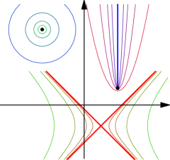
(a) (b)

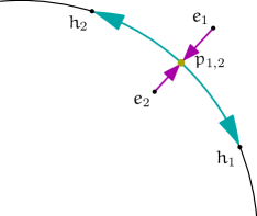
Figure 12: (a) Zero-radius cycles in elliptic (black point) and hyperbolic (the red light cone). Infinitesimal radius parabolic cycle is the blue vertical ray starting at the focus.
(b) Elliptic-parabolic-hyperbolic phase transition between fixed points of the subgroup $K$.

It is easy to see that infinitesimal radius cycles has properties similar to zero-radius ones, cf. Lemma 3.15.

Lemma 6.5.

The image of $SL_{2}{}(\mathbb{R}{})$-action on an infinitesimal radius cycle (6.1) by conjugation (3.4) is an infinitesimal radius cycle of the same order.

Image of an infinitesimal cycle under cycle conjugation is an infinitesimal cycle of the same or lesser order.

Proof 6.6.

These are calculations done in GiNaC, see [Kisil05b]*§ LABEL:G-sec:mobi-transf-infin.

The consideration of infinitesimal numbers in the elliptic and hyperbolic case should not bring any advantages since the (leading) quadratic terms in these cases are non-zero. However non-Archimedean numbers in the parabolic case provide a more intuitive and efficient presentation. For example zero-radius cycles are not helpful for the parabolic Cayley transform (see subsection 8.2) but infinitesimal cycles are their successful replacements.

The second part of the following result is a useful substitution for Lem. 4.6.

Lemma 6.7.

Let ${C^{s}_{\breve{\sigma}}}$ be the infinitesimal cycle (6.1) and ${\breve{C}^{s}_{\breve{\sigma}}}=(k,l,n,m)$ be a generic cycle. Then

1. The orthogonality condition (4.2) ${C^{s}_{\breve{\sigma}}}\perp{\breve{C}^{s}_{\breve{\sigma}}}$ and the f-orthogonality (4.12) ${\breve{C}^{s}_{\breve{\sigma}}}\dashv{C^{s}_{\breve{\sigma}}}$ both are given by:

   $$ku_{0}^{2}-2lu_{0}+m=O(\varepsilon).$$

   In other words the cycle ${\breve{C}^{s}_{\breve{\sigma}}}$ has root $u_{0}$ in the parabolic space.

2. The f-orthogonality (4.12) ${C^{s}_{\breve{\sigma}}}\dashv{\breve{C}^{s}_{\breve{\sigma}}}$ is given by:

   $$ku_{0}^{2}-2lu_{0}-2nv_{0}+m=O(\varepsilon).$$ (6.4)

   In other words the cycle ${\breve{C}^{s}_{\breve{\sigma}}}$ passes focus $(u_{0},v_{0})$ of the infinitesimal cycle in the parabolic space.

Proof 6.8.

These are GiNaC calculations [Kisil05b]*§ LABEL:G-sec:orth-with-infin.

It is interesting to note that the exotic f-orthogonality became warranted replacement of the usual one for the infinitesimal cycles.

6.2 Infinitesimal Conformality

An intuitive idea of conformal maps, which is oftenly provided in the complex analysis textbooks for illustration purposes, is “they send small circles into small circles with respective centres”. Using infinitesimal cycles one can turn it into a precise definition.

Definition 6.9.

A map of a region of $\mathbb{R}^{a}{}$ to another region is $l$-infinitesimally conformal for a length $l$ (in the sense of Defn. 5.5) if for any $l$-infinitesimal cycle:

1. Its image is an $l$-infinitesimal cycle of the same order;

2. The image of its centre/focus is displaced from the centre/focus of its image by an infinitesimal number of a greater order than its radius.

Remark 6.10.

Note that in comparison with Defn. 5.14 we now work “in the opposite direction”: former we had the fixed group of motions and looked for corresponding conformal lengths/distances, now we take a distance/length (encoded in the infinitesimally equidistant cycle) and check which motions respect it.

Natural conformalities for lengths from centre in the elliptic and parabolic cases are already well studied. Thus we are mostly interested here in conformality in the parabolic case, where lengths from focus are better suited. The image of an infinitesimal cycle (6.1) under $SL_{2}{}(\mathbb{R}{})$-action is a cycle, moreover its is again an infinitesimal cycle of the same order by Lemma 6.5. This provides the first condition of Defn. 6.9. The second part is delivered by the following statement:

Proposition 6.11.

Let ${\breve{C}^{s}_{\breve{\sigma}}}$ be the image under $g\in SL_{2}{}(\mathbb{R}{})$ of an infinitesimal cycle ${C^{s}_{\breve{\sigma}}}$ from (6.1). Then $\mathring{\sigma}$-focus of ${\breve{C}^{s}_{\breve{\sigma}}}$ is displaced from $g(u_{0},v_{0})$ by infinitesimals of order $\varepsilon^{2}$ (while both cycles have $\breve{\sigma}$-radius of order $\varepsilon$).

Consequently $SL_{2}{}(\mathbb{R}{})$-action is infinitesimally conformal in the sense of Defn. 6.9 with respect to the length from focus (Defn. 5.5) for all combinations of $\sigma$, $\breve{\sigma}$ and $\mathring{\sigma}$.

Proof 6.12.

These are GiNaC calculations [Kisil05b]*§ LABEL:G-sec:mobi-transf-infin.

Infinitesimal conformality seems intuitively to be close to Defn. 5.14. Thus it is desirable to give a reason for the absence of exclusion clauses in Prop. 6.11 in comparison to Prop. 5.15.3. As shows calculations [Kisil05b]*§ LABEL:G-sec:check-conformity the limit (5.9) at point $y_{0}=u_{0}e_{0}+v_{0}e_{1}$ do exist but depends from the direction $y=ue_{0}+ve_{1}$:

$$\lim_{t\rightarrow 0}\frac{d(g\cdot y_{0},g\cdot(y_{0}+ty))}{d(y_{0},y_{0}+ty)}=\frac{1}{(d+cu_{0})^{2}+\sigma c^{2}v_{0}^{2}-2Kcv_{0}(d+cu_{0})},$$ (6.5)

where $\displaystyle K=\frac{u}{v}$ and $g=\begin{pmatrix}a&b\\ c&d\end{pmatrix}$. However if we consider points  (6.3) of the infinitesimal cycle then $\displaystyle K=\frac{\varepsilon u}{v_{0}u^{2}}=\frac{\varepsilon}{v_{0}u}$. Thus the value of the limit (6.5) at the infinitesimal scale is independent from $y=ue_{0}+ve_{1}$. It also coincides (up to an infinitesimal number) with the value in (5.10).

Remark 6.13.

There is another connection between parabolic function theory and non-standard analysis. As was mentioned in § 2, the Clifford algebra ${\mathcal{C}\kern-1.19995pt\ell(p)}$ corresponds to the set of dual numbers $u+\varepsilon v$ with $\varepsilon^{2}=0$ [Yaglom79]*Supl. C. On the other hand we may consider the set of numbers $u+\varepsilon v$ within the non-standard analysis, with $\varepsilon$ being an infinitesimal. In this case $\varepsilon^{2}$ is a higher order infinitesimal than $\varepsilon$ and effectively can be treated as $0$ at infinitesimal scale of $\varepsilon$, i.e. we again get the dual numbers condition $\varepsilon^{2}=0$. This explains why many results of differential calculus can be naturally deduced within dual numbers framework [CatoniCannataNichelatti04].

Infinitesimal cycles are also a convenient tool for calculations of invariant measures, Jacobians, etc.

7 Global Properties

So far we were interested in individual properties of cycles and local properties of the point space. Now we describe some global properties which are related to the set of cycles as the whole.

7.1 Compactification of $\mathbb{R}^{\sigma}{}$

Giving Definition 3.1 of maps $Q$ and $M$ we did not consider properly their domains and ranges. For example, the image of $(0,0,0,1)\in\mathbb{P}^{3}{}$, which is transformed by $Q$ to the equation $1=0$, is not a valid conic section in $\mathbb{R}^{\sigma}{}$. We also did not investigate yet accurately singular points of the Möbius map (2.3). It turns out that both questions are connected.

One of the standard approaches [Olver99]*§ 1 to deal with singularities of the Möbius map is to consider projective coordinates on the plane. Since we have already a projective space of cycles, we may use it as a model for compactification which is even more appropriate. The identification of points with zero-radius cycles plays an important rôle here.

Definition 7.1.

The only irregular point $(0,0,0,1)\in\mathbb{P}^{3}{}$ of the map $Q$ is called zero-radius cycle at infinity and denoted by $Z_{\infty}$.

The following results are easily obtained by direct calculations even without a computer:

Lemma 7.2.

1. $Z_{\infty}$ is the image of the zero-radius cycle $Z_{(0,0)}=(1,0,0,0)$ at the origin under reflection (inversion) into the unit cycle $(1,0,0,-1)$, see blue cycles in Fig. 9(b)-(d).

2. The following statements are equivalent

   1. A point $(u,v)\in\mathbb{R}^{\sigma}{}$ belongs to the zero-radius cycle $Z_{(0,0)}$ centred at the origin;

   2. The zero-radius cycle $Z_{(u,v)}$ is $\sigma$-orthogonal to zero-radius cycle $Z_{(0,0)}$;

   3. The inversion $z\mapsto\frac{1}{z}$ in the unit cycle is singular in the point $(u,v)$;

   4. The image of $Z_{(u,v)}$ under inversion in the unit cycle is orthogonal to $Z_{\infty}$.

   If any from the above is true we also say that image of $(u,v)$ under inversion in the unit cycle belongs to zero-radius cycle at infinity.

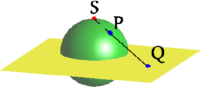
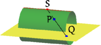
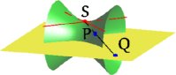
(a) (b) (c)

Figure 13: Compactification of $\mathbb{R}^{\sigma}{}$ and stereographic projections.

In the elliptic case the compactification is done by addition to $\mathbb{R}^{e}{}$ a point $\infty$ at infinity, which is the elliptic zero-radius cycle. However in the parabolic and hyperbolic cases the singularity of the Möbius transform is not localised in a single point—the denominator is a zero divisor for the whole zero-radius cycle. Thus in each EPH case the correct compactification is made by the union $\mathbb{R}^{\sigma}{}\cup Z_{\infty}$.

It is common to identify the compactification ${\dot{\mathbb{R}}^{e}}$ of the space $\mathbb{R}^{e}{}$ with a Riemann sphere. This model can be visualised by the stereographic projection, see [BergerII]*§ 18.1.4 and Fig. 13(a). A similar model can be provided for the parabolic and hyperbolic spaces as well, see [HerranzSantander02b] and Fig. 13(b),(c). Indeed the space $\mathbb{R}^{\sigma}{}$ can be identified with a corresponding surface of the constant curvature: the sphere ($\sigma=-1$), the cylinder ($\sigma=0$), or the one-sheet hyperboloid ($\sigma=1$). The map of a surface to $\mathbb{R}^{\sigma}{}$ is given by the polar projection, see [HerranzSantander02b]*Fig. 1 and Fig. 13(a)-(c). These surfaces provide “compact” model of the corresponding $\mathbb{R}^{\sigma}{}$ in the sense that Möbius transformations which are lifted from $\mathbb{R}^{\sigma}{}$ by the projection are not singular on these surfaces.

However the hyperbolic case has its own caveats which may be easily oversight as in the paper cited above, for example. A compactification of the hyperbolic space $\mathbb{R}^{h}{}$ by a light cone (which the hyperbolic zero-radius cycle) at infinity will indeed produce a closed Möbius invariant object. However it will not be satisfactory for some other reasons explained in the next subsection.

7.2 (Non)-Invariance of The Upper Half-Plane

The important difference between the hyperbolic case and the two others is that

Lemma 7.3.

In the elliptic and parabolic cases the upper halfplane in $\mathbb{R}^{\sigma}{}$ is preserved by Möbius transformations from $SL_{2}{}(\mathbb{R}{})$. However in the hyperbolic case any point $(u,v)$ with $v>0$ can be mapped to an arbitrary point $(u^{\prime},v^{\prime})$ with $v^{\prime}\neq 0$.

This is illustrated by Fig. 3: any cone from the family (2.7) is intersecting the both planes $EE^{\prime}$ and $PP^{\prime}$ over a connected curve, however intersection with the plane $HH^{\prime}$ has two branches.

The lack of invariance in the hyperbolic case has many important consequences in seemingly different areas, for example:

$t=0$

$\to$ $t=e^{-3}$ $\to$ $t=e^{-2}$ $\to$ $t=e^{-1}$
$t=1$ $\to$ $t=e$ $\to$ $t=e^{2}$ $\to$ $t=e^{3}$

Figure 14: Eight frames from a continuous transformation from future to the past parts of the light cone.

Geometry

$\mathbb{R}^{h}{}$ is not split by the real axis into two disjoint pieces: there is a continuous path (through the light cone at infinity) from the upper half-plane to the lower which does not cross the real axis (see $\sin$-like curve joined two sheets of the hyperbola in Fig. 15(a)).

Physics

There is no Möbius invariant way to separate “past” and “future” parts of the light cone [Segal76], i.e. there is a continuous family of Möbius transformations reversing the arrow of time. For example, the family of matrices $\begin{pmatrix}1&-te_{1}\\ te_{1}&1\end{pmatrix}$, $t\in[0,\infty)$ provides such a transformation. Fig. 14 illustrates this by corresponding images for eight subsequent values of $t$.

Analysis

There is no a possibility to split $L_{2}{}(\mathbb{R}{})$ space of function into a direct sum of the Hardy type space of functions having an analytic extension into the upper half-plane and its non-trivial complement, i.e. any function from $L_{2}{}(\mathbb{R}{})$ has an “analytic extension” into the upper half-plane in the sense of hyperbolic function theory, see [Kisil97c].

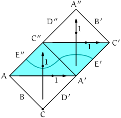
(a)               (b)

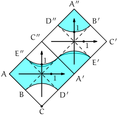
Figure 15: Hyperbolic objects in the double cover of $\mathbb{R}^{h}{}$:
(a) the “upper” half-plane;  (b) the unit circle.

All the above problems can be resolved in the following way [Kisil97c]*§ A.3. We take two copies $\mathbb{R}^{h}_{+}{}$ and $\mathbb{R}^{h}_{-}{}$ of $\mathbb{R}^{h}{}$, depicted by the squares $ACA^{\prime}C^{\prime\prime}$ and $A^{\prime}C^{\prime}A^{\prime\prime}C^{\prime\prime}$ in Fig. 15 correspondingly. The boundaries of these squares are light cones at infinity and we glue $\mathbb{R}^{h}_{+}{}$ and $\mathbb{R}^{h}_{-}{}$ in such a way that the construction is invariant under the natural action of the Möbius transformation. That is achieved if the letters $A$, $B$, $C$, $D$, $E$ in Fig. 15 are identified regardless of the number of primes attached to them. The corresponding model through a stereographic projection is presented on Fig. 16, compare with Fig. 13(c).

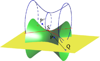
Figure 16: Double cover of the hyperbolic space, cf. Fig. 13(c). The second hyperboloid is shown as a blue skeleton. It is attached to the first one along the light cone at infinity, which is represented by two red lines.

This aggregate denoted by ${\widetilde{\mathbb{R}}^{h}}$ is a two-fold cover of $\mathbb{R}^{h}{}$. The hyperbolic “upper” half-plane in ${\widetilde{\mathbb{R}}^{h}}$ consists of the upper halfplane in $\mathbb{R}^{h}_{+}{}$ and the lower one in $\mathbb{R}^{h}_{-}{}$. A similar conformally invariant two-fold cover of the Minkowski space-time was constructed in [Segal76]*§ III.4 in connection with the red shift problem in extragalactic astronomy.

Remark 7.4.

1. The hyperbolic orbit of the $K$ subgroup in the ${\widetilde{\mathbb{R}}^{h}}$ consists of two branches of the hyperbola passing through $(0,v)$ in $\mathbb{R}^{h}_{+}{}$ and $(0,-v^{-1})$ in $\mathbb{R}^{h}_{-}{}$, see Fig. 15. If we watch the rotation of a straight line generating a cone (2.7) then its intersection with the plane $HH^{\prime}$ on Fig. 3(d) will draw the both branches. As mentioned in Rem. 2.6.2 they have the same focal length.

2. The “upper” halfplane is bounded by two disjoint “real” axes denoted by $AA^{\prime}$ and $C^{\prime}C^{\prime\prime}$ in Fig. 15.

For the hyperbolic Cayley transform in the next subsection we need the conformal version of the hyperbolic unit disk. We define it in ${\widetilde{\mathbb{R}}^{h}}$ as follows:

$${\widetilde{\mathbb{D}}} = \{(ue_{0}+ve_{1})\,\mid\,u^{2}-v^{2}>-1,\ u\in\mathbb{R}^{h}_{+}{}\}$$

$${}\cup\{(ue_{0}+ve_{1})\,\mid\,u^{2}-v^{2}<-1,\ u\in\mathbb{R}^{h}_{-}{}\}.$$

It can be shown that ${\widetilde{\mathbb{D}}}$ is conformally invariant and has a boundary ${\widetilde{\mathbb{T}}}$—two copies of the unit circles in $\mathbb{R}^{h}_{+}{}$ and $\mathbb{R}^{h}_{-}{}$. We call ${\widetilde{\mathbb{T}}}$ the (conformal) unit circle in $\mathbb{R}^{h}{}$. Fig. 15(b) illustratesthe geometry of the conformal unit disk in ${\widetilde{\mathbb{R}}^{h}}$ in comparison with the “upper” half-plane.

8 The Cayley Transform and the Unit Cycle

The upper half-plane is the universal starting point for an analytic function theory of any EPH type. However universal models are rarely best suited to particular circumstances. For many reasons it is more convenient to consider analytic functions in the unit disk rather than in the upper half-plane, although both theories are completely isomorphic, of course. This isomorphism is delivered by the Cayley transform. Its drawback is that there is no a “universal unit disk”, in each EPH case we obtain something specific from the same upper half-plane.

8.1 Elliptic and Hyperbolic Cayley Transforms

In the elliptic and hyperbolic cases [Kisil97c] the Cayley transform is given by the matrix $C=\begin{pmatrix}1&-e_{1}\\ \sigma e_{1}&1\end{pmatrix}$, where $\sigma=e_{1}^{2}$ (2.1) and $\det C=2$. It can be applied as the Möbius transformation

$$\begin{pmatrix}1&-e_{1}\\ \sigma e_{1}&1\end{pmatrix}:\ w=(ue_{0}+ve_{1})\mapsto Cw=\frac{(ue_{0}+ve_{1})-e_{1}}{\sigma e_{1}(ue_{0}+ve_{1})+1}$$ (8.1)

to a point $(ue_{0}+ve_{1})\in\mathbb{R}^{\sigma}{}$. Alternatively it acts by conjugation $g_{C}=\frac{1}{2}CgC^{-1}$ on an element $g\in SL_{2}{}(\mathbb{R}{})$:

$$g_{C}=\frac{1}{2}\begin{pmatrix}1&-e_{1}\\ \sigma e_{1}&1\end{pmatrix}\begin{pmatrix}a&be_{0}\\ -ce_{0}&d\end{pmatrix}\begin{pmatrix}1&e_{1}\\ -\sigma e_{1}&1\end{pmatrix}$$ (8.2)

The connection between the two forms (8.1) and (8.2) of the Cayley transform is given by $g_{C}Cw=C(gw)$, i.e. $C$ intertwines the actions of $g$ and $g_{C}$.

The Cayley transform $(u^{\prime}e_{0}+v^{\prime}e_{1})=C(ue_{0}+ve_{1})$ in the elliptic case is very important [Lang85]*§ IX.3 [MTaylor86]*Ch. 8, (1.12) both for complex analysis and representation theory of $SL_{2}{}(\mathbb{R}{})$. The transformation $g\mapsto g_{C}$ (8.2) is an isomorphism of the groups $SL_{2}{}(\mathbb{R}{})$ and $\mathrm{SU}(1,1)$ namely in ${\mathcal{C}\kern-1.19995pt\ell(e)}$ we have

$$g_{C}=\frac{1}{2}\begin{pmatrix}f&h\\ -h&f\end{pmatrix},\textrm{ with }f=(a+d)-(b-c)e_{1}e_{0}\textrm{ and }h=(a-d)e_{1}+(b+c)e_{0}.$$ (8.3)

Under the map $\mathbb{R}^{e}{}\to\mathbb{C}{}$ (2.2) this matrix becomes $\begin{pmatrix}\alpha&\beta\\ \bar{\beta}&\bar{\alpha}\end{pmatrix}$, i.e. the standard form of elements of $\mathrm{SU}(1,1)$ [Lang85]*§ IX.1 [MTaylor86]*Ch. 8, (1.11).

The images of elliptic actions of subgroups $A$, $N$, $K$ are given in Fig. 17($E$). The types of orbits can be easily distinguished by the number of fixed points on the boundary: two, one and zero correspondingly. Although a closer inspection demonstrate that there are always two fixed points, either:

• one strictly inside and one strictly outside of the unit circle; or

• one double fixed point on the unit circle; or

• two different fixed points exactly on the circle.

Consideration of Figure 12(b) shows that the parabolic subgroup $N$ is like a phase transition between the elliptic subgroup $K$ and hyperbolic $A$, cf. (1.1).

In some sense the elliptic Cayley transform swaps complexities: by contract to the upper half-plane the $K$-action is now simple but $A$ and $N$ are not. The simplicity of $K$ orbits is explained by diagonalisation of matrices:

$$\frac{1}{2}\begin{pmatrix}1&-e_{1}\\ -e_{1}&1\end{pmatrix}\begin{pmatrix}\cos\phi&-e_{0}\sin\phi\\ -e_{0}\sin\phi&\cos\phi\end{pmatrix}\begin{pmatrix}1&e_{1}\\ e_{1}&1\end{pmatrix}=\begin{pmatrix}\varepsilon^{\mathrm{i}\phi}&0\\ 0&\varepsilon^{\mathrm{i}\phi}\end{pmatrix},$$ (8.4)

where $\mathrm{i}=e_{1}e_{0}$ behaves as the complex imaginary unit, i.e. $\mathrm{i}^{2}=-1$.

A hyperbolic version of the Cayley transform was used in [Kisil97c]. The above formula (8.2) in $\mathbb{R}^{h}{}$ becomes as follows:

$$g_{C}=\frac{1}{2}\begin{pmatrix}f&h\\ h&f\end{pmatrix},\textrm{ with }f=a+d-(b+c)e_{1}e_{0}\textrm{ and }h=(d-a)e_{1}+(b-c)e_{0},$$ (8.5)

with some subtle differences in comparison with (8.3). The corresponding $A$, $N$ and $K$ orbits are given on Fig. 17($H$). However there is an important distinction between the elliptic and hyperbolic cases similar to one discussed in subsection 7.2.

($E$)    
($P_{e}$)
($P_{p}$)
($P_{e}$)
($H$)

Figure 17: The unit disks and orbits of subgroups $A$, $N$ and $K$:
($E$): The elliptic unit disk;
($P_{e}$), ($P_{p}$), ($P_{h}$): The elliptic, parabolic and hyeprbolic flavour of the parabolic unit disk (the pure parabolic type ($P_{p}$) transform is very similar with Figs. 1 and 2($K_{p}$)).
   ($H$): The hyperbolic unit disk.

Lemma 8.1.

1. In the elliptic case the “real axis” $U$ is transformed to the unit circle and the upper half-plane—to the unit disk:

   $$\{(u,v)\,\mid\,v=0\} \to \{(u^{\prime},v^{\prime})\,\mid\,l^{2}_{c_{e}}(u^{\prime}e_{0}+v^{\prime}e_{1})=u^{\prime 2}+v^{\prime 2}=1\}$$ (8.6)

   $$\{(u,v)\,\mid\,v>0\} \to \{(u^{\prime},v^{\prime})\,\mid\,l^{2}_{c_{e}}(u^{\prime}e_{0}+v^{\prime}e_{1})=u^{\prime 2}+v^{\prime 2}<1\},$$ (8.7)

   where the length from centre $l^{2}_{c_{e}}$ is given by (5.5) for $\sigma=\breve{\sigma}=-1$.

   On both sets $SL_{2}{}(\mathbb{R}{})$ acts transitively and the unit circle is generated, for example, by the point $(0,1)$ and the unit disk is generated by $(0,0)$.

2. In the hyperbolic case the “real axis” $U$ is transformed to the hyperbolic unit circle:

   $$\{(u,v)\,\mid\,v=0\}\to\{(u^{\prime},v^{\prime})\,\mid\,l^{2}_{c_{h}}(u^{\prime},v^{\prime})=u^{\prime 2}-v^{\prime 2}=-1\},$$ (8.8)

   where the length from centre $l^{2}_{c_{h}}$ is given by (5.5) for $\sigma=\breve{\sigma}=1$.

   On the hyperbolic unit circle $SL_{2}{}(\mathbb{R}{})$ acts transitively and it is generated, for example, by point $(0,1)$.

   $SL_{2}{}(\mathbb{R}{})$ acts also transitively on the whole complement

   $$\{(u^{\prime},v^{\prime})\,\mid\,l^{2}_{c_{h}}(u^{\prime}e_{0}+v^{\prime}e_{1})\neq-1\}$$

   to the unit circle, i.e. on its “inner” and “outer” parts together.

The last feature of the hyperbolic Cayley transform can be treated in a way described in the end of subsection 7.2, see also Fig. 15(b). With such an arrangement the hyperbolic Cayley transform maps the “upper” half-plane from Fig. 15(a) onto the “inner” part of the unit disk from Fig. 15(b) .

One may wish that the hyperbolic Cayley transform diagonalises the action of subgroup $A$, or some conjugated, in a fashion similar to the elliptic case (8.4) for $K$. Geometrically it will correspond to hyperbolic rotations of hyperbolic unit disk around the origin. Since the origin is the image of the point $e_{1}$ in the upper half-plane under the Cayley transform, we will use the fix subgroup $A^{\prime}_{h}$ (2.9) conjugated to $A$ by $\begin{pmatrix}1&e_{0}\\ e_{0}&1\end{pmatrix}\in SL_{2}{}(\mathbb{R}{})$. Under the Cayley map (8.5) the subgroup $A^{\prime}_{h}$ became, cf. [Kisil97c]*(3.6–3.7):

$$\frac{1}{2}\begin{pmatrix}1&e_{1}\\ -e_{1}&1\end{pmatrix}\begin{pmatrix}\cosh t&-e_{0}\sinh t\\ e_{0}\sinh t&\cosh t\end{pmatrix}\begin{pmatrix}1&-e_{1}\\ e_{1}&1\end{pmatrix}=\begin{pmatrix}\exp(e_{1}e_{0}t)&0\\ 0&\exp(e_{1}e_{0}t)\end{pmatrix},$$

where $\exp(e_{1}e_{0}t)=cosh(t)+e_{1}e_{0}sinh(t)$. This obviously corresponds to hyperbolic rotations of $\mathbb{R}^{h}{}$. Orbits of the fix subgroups $A^{\prime}_{h}$, $N^{\prime}_{p}$ and $K^{\prime}_{e}$ from Lem. 2.7 under the Cayley transform are shown on Fig. 18, which should be compared with Fig. 4. However the parabolic Cayley transform requires a separate discussion.

Figure 18: Concentric/confocal orbits of one parametric subgroups, cf. Fig. 4

8.2 Parabolic Cayley Transforms

This case benefits from a bigger variety of choices. The first natural attempt to define a Cayley transform can be taken from the same formula (8.1) with the parabolic value $\sigma=0$. The corresponding transformation defined by the matrix $\begin{pmatrix}1&-e_{1}\\ 0&1\end{pmatrix}$ and defines the shift one unit down.

However within the framework of this paper a more general version of parabolic Cayley transform is possible. It is given by the matrix

$$C_{\breve{\sigma}}=\begin{pmatrix}1&-e_{1}\\ \breve{\sigma}e_{1}&1\end{pmatrix},\qquad\text{ where }\breve{\sigma}=-1,0,1\text{ and }\det C_{\breve{\sigma}}=1\text{ for all }\breve{\sigma}.$$ (8.9)

Here $\breve{\sigma}=-1$ corresponds to the parabolic Cayley transform $P_{e}$ with the elliptic flavour, $\breve{\sigma}=1$ — to the parabolic Cayley transform $P_{h}$ with the hyperbolic flavour, cf. [Kisil04b]*§ 2.6. Finally the parabolic-parabolic transform is given by an upper-triangular matrix from the end of the previous paragraph.

Fig. 17 presents these transforms in rows ($P_{e}$), ($P_{p}$) and ($P_{h}$) correspondingly. The row ($P_{p}$) almost coincides with Figs. 1($A_{a}$), 1($N_{a}$) and 2($K_{p}$). Consideration of Fig. 17 by columns from top to bottom gives an impressive mixture of many common properties (e.g. the number of fixed point on the boundary for each subgroup) with several gradual mutations.

The description of the parabolic “unit disk” admits several different interpretations in terms lengths from Defn. 5.5.

Lemma 8.2.

Parabolic Cayley transform $P_{\breve{\sigma}}$ as defined by the matrix $C_{\breve{\sigma}}$ (8.9) acts on the $V$-axis always as a shift one unit down.

Its image can be described in term of various lengths as follows:

1. $P_{\breve{\sigma}}$ for $\breve{\sigma}\neq 0$ transforms the “real axis” $U$ to the p-cycle with the p-length squared $-\breve{\sigma}$ from its e-centre $(0,-\frac{\breve{\sigma}}{2})$, cf. (8.6):

   $$\{(u,v)\,\mid\,v=0\}\to\{(u^{\prime},v^{\prime})\,\mid\,l_{c_{e}}^{2}((0,-\frac{\breve{\sigma}}{2}),(u^{\prime},v^{\prime}))\cdot(-\breve{\sigma})=1\},$$ (8.10)

   where $l_{c_{e}}^{2}((0,-\frac{\breve{\sigma}}{2}),(u^{\prime},v^{\prime}))=u^{\prime 2}+\breve{\sigma}v^{\prime}$, see (5.5).

   The image of upper halfplane is:

   $$\{(u,v)\,\mid\,v>0\}\to\{(u^{\prime},v^{\prime})\,\mid\,l_{c_{e}}^{2}((0,-\frac{\breve{\sigma}}{2}),(u^{\prime},v^{\prime}))\cdot(-\breve{\sigma})<1\}.$$ (8.11)

2. $P_{\breve{\sigma}}$ with $\breve{\sigma}\neq 0$ transforms the “real axis” $U$ to the p-cycle with p-length squared $-\breve{\sigma}$ (5.7) from its h-focus $(0,-1-\frac{\breve{\sigma}}{4})$, and the upper half-plane—to the “interior” part of it, cf. (8.6):

   $$\{(u,v)\,\mid\,v=0\} \to \{(u^{\prime},v^{\prime})\,\mid\,l_{f_{h}}^{2}((0,{\textstyle-1-\frac{\breve{\sigma}}{4}}),(u^{\prime},v^{\prime}))\cdot(-\breve{\sigma})=1\},$$ (8.12)

   $$\{(u,v)\,\mid\,v>0\} \to \{(u^{\prime},v^{\prime})\,\mid\,l_{f_{h}}^{2}((0,{\textstyle-1-\frac{\breve{\sigma}}{4}}),(u^{\prime},v^{\prime}))\cdot(-\breve{\sigma})<1\}.$$ (8.13)

3. $P_{\breve{\sigma}}$ transforms the “real axis” $U$ to the cycle with p-length $-\breve{\sigma}$ from its p-focus $(0,-1)$, and the upper half-plane—to the “interior” part of it, cf. (8.6):

   $$\{(u,v)\,\mid\,v=0\} \to \{(u^{\prime},v^{\prime})\,\mid\,l_{f_{p}}^{2}((0,-1),(u^{\prime},v^{\prime}))\cdot(-\breve{\sigma})=1\},$$ (8.14)

   $$\{(u,v)\,\mid\,v>0\} \to \{(u^{\prime},v^{\prime})\,\mid\,l_{f_{p}}^{2}((0,-1),(u^{\prime},v^{\prime}))\cdot(-\breve{\sigma})<1\},$$ (8.15)

   where $l_{f_{p}}^{2}((0,-1),(u^{\prime},v^{\prime}))=\frac{u^{\prime 2}}{v^{\prime}+1}$ (5.7).

Remark 8.3.

Note that the both elliptic (8.6) and hyperbolic (8.8) unit circle descriptions can be written uniformly with parabolic descriptions (8.10)–(8.14) as

$$\{(u^{\prime},v^{\prime})\,\mid\,l^{2}_{c_{\breve{\sigma}}}(u^{\prime}e_{0}+v^{\prime}e_{1})\cdot(-\breve{\sigma})=1\}.$$

The above descriptions 8.2.1 and 8.2.3 are attractive for reasons given in the following two lemmas. Firstly, the $K$-orbits in the elliptic case (Fig. 18($K_{e}$)) and the $A$-orbits in the hyperbolic case (Fig. 18($A_{h}$)) of Cayley transform are concentric.

Lemma 8.4.

$N$-orbits in the parabolic cases (Fig. 17($N_{P_{e}}$, $N_{P_{p}}$, $N_{P_{h}}$)) are concentric parabolas (or straight lines) in the sense of Defn. 2.12 with e-centres at $(0,\frac{1}{2})$, $(0,\infty)$, $(0,-\frac{1}{2})$ correspondingly.

Secondly, Calley images of the fix subgroups’ orbits in elliptic and hyperbolic spaces in Fig. 18($A_{h}$) and ($K_{e}$) are equidistant from the origin in the corresponding metrics.

Lemma 8.5.

The Cayley transform of orbits of the parabolic fix subgroup in Fig. 18($N^{\prime}_{P_{e}}$) are parabolas consisting of points on the same $l_{f_{p}}$-length (5.6) from the point $(0,-1)$, cf. 8.2.3.

Note that parabolic rotations of the parabolic unit disk are incompatible with the algebraic structure provided by the algebra of dual numbers. However we can introduce [Kisil07a, Kisil09c] a linear algebra structure and vector multiplication which will rotationally invariant under action of subgroups $N$ and $N^{\prime}$.

Remark 8.6.

We see that the varieties of possible Cayley transforms in the parabolic case is bigger than in the two other cases. It is interesting that this parabolic richness is a consequence of the parabolic degeneracy of the generator $e_{1}^{2}=0$. Indeed for both the elliptic and the hyperbolic signs in $e_{1}^{2}=\pm 1$ only one matrix (8.1) out of two possible $\begin{pmatrix}1&e_{1}\\ \pm\sigma e_{1}&1\end{pmatrix}$ has a non-zero determinant. And only for the degenerate parabolic value $e_{1}^{2}=0$ both these matrices are non-singular!

8.3 Cayley Transforms of Cycles

The next natural step within the SFSCc is to expand the Cayley transform to the space of cycles. This is performed as follows:

Lemma 8.7.

Let ${C^{s}_{a}}$ be a cycle in $\mathbb{R}^{\sigma}{}$.

• In the elliptic or hyperbolic cases the Cayley transform maps a cycle ${C^{s}_{\breve{\sigma}}}$ to the composition of its inversion with the reflection ${\hat{C}^{s}_{\breve{\sigma}}}{C^{s}_{\breve{\sigma}}}{\hat{C}^{s}_{\breve{\sigma}}}$ in the cycle ${C^{s}_{\breve{\sigma}}}$, where ${\hat{C}^{s}_{\breve{\sigma}}}=\begin{pmatrix}\pm\breve{e}_{1}&&1\\ 1&&\mp\breve{e}_{1}\end{pmatrix}$ with $\breve{\sigma}=\pm 1$ (see the first and last drawings on Fig. 19).

• In the parabolic case the Cayley transform maps a cycle $(k,l,n,m)$ to the cycle $(k-2\breve{\sigma}n,l,n,m+2\breve{\sigma}n)$.

The above extensions of the Cayley transform to the cycles space is linear, however in the parabolic case it is not expressed as a similarity of matrices (reflections in a cycle). This can be seen, for example, from the fact that the parabolic Cayley transform does not preserve the zero-radius cycles represented by matrices with zero p-determinant.

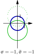
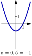
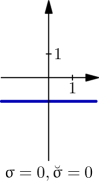
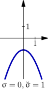
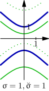
Figure 19: Cayley transforms in elliptic ($\sigma=-1$), parabolic ($\sigma=0$) and hyperbolic ($\sigma=1$) spaces. On the each picture the reflection of the real line in the green cycles (drawn continuously or dotted) is the is the blue “unit cycle”. Reflections in the solidly drawn cycles send the upper half-plane to the unit disk, reflection in the dashed cycle—to its complement. Three Cayley transforms in the parabolic space ($\sigma=0$) are themselves elliptic ($\breve{\sigma}=-1$), parabolic ($\breve{\sigma}=0$) and hyperbolic ($\breve{\sigma}=1$), giving a gradual transition between proper elliptic and hyperbolic cases.

Since orbits of all subgroups in $SL_{2}{}(\mathbb{R}{})$ as well as their Cayley images are cycles in the corresponding metrics we may use Lem. (p)(p) to prove the following statements (in addition to Lem. 8.4):

Corollary 8.8.

1. $A$-orbits in transforms $P_{e}$ and $P_{h}$ are segments of parabolas with the focal length $\frac{1}{2}$ passing through $(0,-\frac{1}{2})$. Their vertices belong to two parabolas $v=\frac{1}{2}(-x^{2}-1)$ and $v=\frac{1}{2}(x^{2}-1)$ correspondingly, which are boundaries of parabolic circles in $P_{h}$ and $P_{e}$ (note the swap!).

2. $K$-orbits in transform $P_{e}$ are parabolas with focal length less than $\frac{1}{2}$ and in transform $P_{h}$—with inverse of focal length bigger than $-2$.

Since the action of parabolic Cayley transform on cycles does not preserve zero-radius cycles one shall better use infinitesimal-radius cycles from § 6.1 instead. First of all images of infinitesimal cycles under parabolic Cayley transform are infinitesimal cycles again [Kisil05b]*§ LABEL:G-sec:cayl-transf-infin, secondly Lemma 6.7.2 provides a useful expression of concurrence with infinitesimal cycle focus through f-orthogonality. Although f-orthogonality is not preserved by the Cayley transform (p)(p) for generic cycles it did for the infinitesimal ones, see [Kisil05b]*§ LABEL:G-sec:cayl-transf-infin:

Lemma 8.9.

An infinitesimal cycle ${C^{a}_{\breve{\sigma}}}$ (6.1) is f-orthogonal (in the sense of Lem. 6.7.2) to a cycle ${\tilde{C}^{a}_{\breve{\sigma}}}$ if and only if the Cayley transform (p)(p) of ${C^{a}_{\breve{\sigma}}}$ is f-orthogonal to the Cayley transform of ${\tilde{C}^{a}_{\breve{\sigma}}}$.

We main observation of this paper is that the potential of the Erlangen programme is still far from exhausting even for two-dimensional geometry.