Conformal invariance of isoradial dimer models
&
the case of triangular quadri-tilings

Abstract

We consider dimer models on graphs which are bipartite, periodic and satisfy a geometric condition called isoradiality, defined in [18]. We show that the scaling limit of the height function of any such dimer model is $1/\sqrt{\pi}$ times a Gaussian free field. Triangular quadri-tilings were introduced in [6]; they are dimer models on a family of isoradial graphs arising form rhombus tilings. By means of two height functions, they can be interpreted as random interfaces in dimension $2+2$. We show that the scaling limit of each of the two height functions is $1/\sqrt{\pi}$ times a Gaussian free field, and that the two Gaussian free fields are independent.

1 Introduction

1.1 Height fluctuations for isoradial dimer models

1.1.1 Dimer models

The setting for this paper is the dimer model. It is a statistical mechanics model representing diatomic molecules adsorbed on the surface of a crystal. An interesting feature of the dimer model is that it is one of the very few statistical mechanics models where exact and explicit results can be obtained, see [14, 15] for an overview. Another very interesting aspect is the alleged conformal invariance of its scaling limit, which is already proved in the domino and $60^{\circ}$-rhombus cases [16, 17, 19]. Theorem 1 of this paper shows this property for a wide class of dimer models containing the above two cases.
In order to give some insight, let us precisely define the setting. The dimer model is in bijection with a mathematical model called the $2$-tiling model representing discrete random interfaces. The system considered for a $2$-tiling model is a planar graph $G$. Configurations of the system, or $2$-tilings, are coverings of $G$ with polygons consisting of pairs of edge-adjacent faces of $G$, also called $2$-tiles, which leave no hole and don’t overlap. The system of the corresponding dimer model is the dual graph $G^{*}$ of $G$. Configurations of the dimer model are perfect matchings of $G^{*}$, that is set of edges covering every vertex exactly once. Perfect matchings of $G^{*}$ determine $2$-tilings of $G$ as explained by the following correspondence. Denote by $f^{*}$ the dual vertex of a face $f$ of $G$, and consider an edge $f^{*}g^{*}$ of $G^{*}$. We say that the $2$-tile of $G$ made of the adjacent faces $f$ and $g$ is the $2$-tile corresponding to the edge $f^{*}g^{*}$. Then $2$-tiles corresponding to edges of a dimer configuration form a $2$-tiling of $G$. Let us denote by ${\cal M}(G^{*})$ the set of dimer configurations of $G^{*}$.
As for all statistical mechanics models, dimer configurations are chosen with respect to the Boltzmann measure defined as follows. Suppose that the graph $G^{*}$ is finite, and that a positive weight function $\nu$ is assigned to edges of $G^{*}$, then each dimer configuration $M$ has an energy, ${\cal E}(M)=-\sum_{e\in M}\log\nu(e)$. The probability of occurrence of the dimer configuration $M$ chosen with respect to the Boltzmann measure $\mu^{1}$ is:

$$\mu^{1}(M)=\frac{e^{-{\cal E}(M)}}{Z(G^{*},\nu)}=\frac{\prod_{e\in M}\nu(e)}{Z(G^{*},\nu)},$$

where $Z(G^{*},\nu)$ is the normalizing constant called the partition function. Using the bijection between dimer configurations and $2$-tilings, $\nu$ can be seen as weighting $2$-tiles, and $\mu^{1}$ as a measure on $2$-tilings of $G$. When the graph $G^{*}$ is infinite, a Gibbs measure is defined to be a probability measure on ${\cal M}(G^{*})$ with the following property: if the matching in an annular region is fixed, then matchings inside and outside of the annulus are independent, moreover the probability of any interior matching $M$ is proportional to $\prod_{e\in M}\nu(e)$. From now on, let us assume that the graph $G$ satisfies condition $(*)$ below:
$(*)$ The graph $G$ is infinite, planar, and simple ($G$ has no loops and no multiple edges); its vertices are of degree $\geq 3$. $G$ is simply connected, i.e. it is the one-skeleton of a simply connected union of faces; and it is made of finitely many different faces, up to isometry.

1.1.2 Isoradial dimer models

This paper actually proves conformal invariance of the scaling limit for a sub-family of all dimer models called isoradial dimer models, introduced by Kenyon in [18]. Much attention has lately been given to isoradial dimer models because of a surprising feature: many statistical mechanics quantities can be computed in terms of the local geometry of the graph. This fact was conjectured in [18], and proved in [7]. The motivation for their study is further enhanced by the fact that the yet classical domino and $60^{\circ}$-rhombus tiling models are examples of isoradial dimer models. Last but not least their understanding allows us to apprehend a random interface model in dimension $2+2$ called the triangular quadri-tiling model introduced in [6], see Section 1.2.1.
Let us now define isoradial dimer models. Speaking in the terminology of $2$-tilings, isoradial $2$-tiling models are defined on graphs $G$ satisfying a geometric condition called isoradiality: all faces of an isoradial graph are inscribable in a circle, and all circumcircles have the same radius, moreover all circumcenters of the faces are contained in the closure of the faces. The energy of configurations is determined by a specific weight function called the critical weight function, see Section 2.1 for definition. Note that if $G$ is an isoradial graph, an isoradial embedding of the dual graph $G^{*}$ is obtained by sending dual vertices to the center of the corresponding faces. Hence, the corresponding dimer model is called an isoradial dimer model.

1.1.3 Height functions

Let $G$ be an isoradial graph, whose dual graph $G^{*}$ is bipartite. Then, by means of the height function, $2$-tilings of $G$ can be interpreted as random discrete $2$-dimensional surfaces in a $3$-dimensional space that are projected orthogonally to the plane. In physics terminology, one speaks of random interfaces in dimension $2+1$. The height function, denoted by $h$, is an ${\mathbb{R}}$-valued function on the vertices of every $2$-tiling of $G$, and is defined in Section 3.

1.1.4 Gaussian free field in the plane

The Gaussian free field in the plane is defined in Section 4. It is a random distribution which assigns to functions ${\varphi}_{1},\ldots,{\varphi}_{k}\in C_{c,0}^{\infty}({\mathbb{R}}^{2})$ (the set of compactly supported smooth functions of ${\mathbb{R}}^{2}$, which have mean $0$), a real Gaussian random vector $(F{\varphi}_{1},\ldots,F{\varphi}_{k})$ whose covariance function is given by

$${\mathbb{E}}(F{\varphi}_{i}F{\varphi}_{j})=\int_{{\mathbb{R}}^{2}}\int_{{\mathbb{R}}^{2}}g(x,y){\varphi}_{i}(x){\varphi}_{j}(y)dx\,dy,$$

where $g(x,y)=-\frac{1}{2\pi}\log|x-y|$ is the Green function of the plane (defined up to an additive constant). The Gaussian free field is conformally invariant [17].

1.1.5 Statement of result

Let $G$ be an isoradial graph, whose dual graph $G^{*}$ is bipartite. Suppose moreover that $G^{*}$ is doubly periodic, i.e. that the graph $G^{*}$ and its vertex-coloring are periodic. Then by Sheffield’s theorem [26], there exists a two-parameter family of translation invariant, ergodic Gibbs measures; let us denote by $\mu$ the unique measure which has minimal free energy per fundamental domain. From now on, we assume that dimer configurations of $G^{*}$ are chosen with respect to the measure $\mu$.
Let us multiply the edge-lengths of the graph $G$ by ${\varepsilon}>0$, this yields a new graph $G^{\varepsilon}$. Let $h^{\varepsilon}$ be the unnormalized height function on $2$-tilings of $G^{\varepsilon}$. An important issue in the study of the dimer model is the understanding of the fluctuations of $h^{\varepsilon}$, as the mesh ${\varepsilon}$ tends to $0$. This question is answered by Theorem 1 below. Define:

$$\begin{array}[]{lccl}H^{\varepsilon}:&C_{c,0}^{\infty}({\mathbb{R}}^{2})&\rightarrow&{\mathbb{R}}\\ &{\varphi}&\longmapsto&\displaystyle H^{\varepsilon}{\varphi}={\varepsilon}^{2}\sum_{v\in V({G^{\varepsilon}})}a(v^{*}){\varphi}(v)h^{\varepsilon}(v),\end{array}$$

where $V({G^{\varepsilon}})$ denotes the set of vertices of the graph ${G^{\varepsilon}}$, and $a(v^{*})$ is the area in $G^{*}$ of the dual face $v^{*}$ of a vertex $v$.

Theorem 1

Consider a graph $G$ satisfying the above assumptions, then $H^{\varepsilon}$ converges weakly in distribution to $\frac{1}{\sqrt{\pi}}$ times a Gaussian free field, that is for every ${\varphi}_{1},\ldots,{\varphi}_{k}\in C_{c,0}^{\infty}({\mathbb{R}}^{2})$, $(H^{\varepsilon}{\varphi}_{1},\ldots,H^{\varepsilon}{\varphi}_{k})$ converges in law (as ${\varepsilon}\rightarrow 0$) to $\frac{1}{\sqrt{\pi}}(F{\varphi}_{1},\ldots,F{\varphi}_{k})$, where $F$ is a Gaussian free field.

$\bullet$ As a direct consequence of Theorem 1, we obtain convergence of the height function of domino and $60^{\circ}$-rhombus tilings chosen with respect to the uniform measure to a Gaussian free field. Note that this result is slightly different than those of [16, 17, 19] since we work on the whole plane, and not on simply connected regions.
$\bullet$ The method for proving Theorem 1 is essentially that of [16], except Lemma 20 which is new. Nevertheless, since we work with a general isoradial graph (and not the square lattice), each step is adapted in a non trivial way.

1.2 The case of triangular quadri-tilings

1.2.1 Triangular quadri-tiling model

An exciting consequence of Theorem 1 is that it allows us to understand height fluctuations in the case of a random interface model in dimension $2+2$, called the triangular quadri-tiling model. It is the first time this type of result can be obtained on such a model.
Let us start by defining triangular quadri-tilings. Consider the set of right triangles whose hypotenuses have length $1$, and whose interior angle is $\pi/3$. Color the vertex at the right angle black, and the other two vertices white. A quadri-tile is a quadrilateral obtained from two such triangles in two different ways: either glue them along a leg of the same length matching the black (white) vertex to the black (white) one, or glue them along the hypotenuse. There are four types of quadri-tiles classified as I, II, III, IV, each of which has four vertices, see Figure 1 (left). A triangular quadri-tiling of the plane is an edge-to-edge tiling of the plane by quadri-tiles that respects the coloring of the vertices, see $T$ of Figure 1 for an example. Let ${\cal Q}$ denote the set of all triangular quadri-tilings of the plane, up to isometry.
In [6], triangular quadri-tilings of ${\cal Q}$ are shown to correspond to two superposed dimer models in the following way, see also Figure 1. Define a lozenge to be a $60^{\circ}$-rhombus. Then triangular quadri-tilings are $2$-tilings of a family of graphs ${\cal L}$ which are lozenge-with-diagonals tilings of the plane, up to isometry. Indeed let $T\in{\cal Q}$ be a triangular quadri-tiling, then on every quadri-tile of $T$ draw the edge separating the two right triangles, this yields a lozenge-with-diagonals tiling $L(T)$ called the underlying tiling. Moreover, the lozenge tiling ${\sf L}(T)$ obtained from $L(T)$ by removing the diagonals, is a $2$-tiling of the equilateral triangular lattice ${\mathbb{T}}$.

Figure 1: Four type of quadri-tiles (left). Triangular quadri-tilings correspond to two superposed dimer models (right).

Note that lozenge-with-diagonals tilings and the equilateral triangular lattice are isoradial graphs. Assigning the critical weight function to edges of their dual graphs, we deduce that triangular quadri-tilings of ${\cal Q}$ correspond to two superposed isoradial dimer models.

1.2.2 Height functions for triangular quadri-tilings

Triangular quadri-tilings are characterized by two height functions in the following way. Let $T\in{\cal Q}$ be a triangular quadri-tiling, then the first height function, denoted by $h_{1}$, assigns to vertices of $T$ the “height” of $T$ interpreted as a $2$-tiling of its underlying lozenge-with-diagonals tiling $L(T)$. The second height function, denoted by $h_{2}$, assigns to vertices of $T$ the height of ${\sf L}(T)$ interpreted as a $2$-tiling of ${\mathbb{T}}$. An example of computation is given in Section 3.3. By means of $h_{1}$ and $h_{2}$, triangular quadri-tilings are interpreted in [6] as discrete random $2$-dimensional surfaces in a $4$-dimensional space that are projected orthogonally to the plane, i.e. in physics terminology, as random interfaces in dimension $2+2$.

1.2.3 Statement of result

The notion of Gibbs measure can be extended naturally to the set ${\cal Q}$ of all triangular quadri-tilings, see Section 2.4. In [7], we give an explicit expression for such a Gibbs measure ${\mathbb{P}}$, and conjecture it to be of minimal free energy per fundamental domain among a four-parameter family of translation invariant, ergodic Gibbs measures. Let us assume that triangular quadri-tilings of ${\cal Q}$ are chosen with respect to the measure ${\mathbb{P}}$.
Corollary 2 below describes the fluctuations of the unnormalized height functions $h_{1}^{\varepsilon}$ and $h_{2}^{\varepsilon}$. Suppose that the equilateral triangular lattice has edge-lengths $1$, and let ${\mathbb{T}}^{\varepsilon}$ be the lattice ${\mathbb{T}}$ whose edge-lengths have been multiplied by ${\varepsilon}$. Observe that vertices of ${\mathbb{T}}$ are vertices of $L$, for every lozenge-with-diagonals tiling $L\in{\cal L}$. For $i=1,2$, and for ${\varphi}\in C_{c,0}^{\infty}({\mathbb{R}}^{2})$ define:

$$H_{i}^{\varepsilon}{\varphi}={\varepsilon}^{2}\sum_{v\in V({\mathbb{T}}^{\varepsilon})}\frac{\sqrt{3}}{2}{\varphi}(v)h_{i}^{\varepsilon}(v),$$

Corollary 2

For $i=1,2$, and every ${\varphi}_{1},\ldots,{\varphi}_{k}\in C_{c,0}^{\infty}({\mathbb{R}}^{2})$, $(H_{i}^{\varepsilon}{\varphi}_{1},\ldots,H_{i}^{\varepsilon}{\varphi}_{k})$ converges in law (as ${\varepsilon}\rightarrow 0$) to $\frac{1}{\sqrt{\pi}}(F_{i}{\varphi}_{1},\ldots,F_{i}{\varphi}_{k})$, where $F_{i}$ is a Gaussian free field. Moreover, $F_{1}$ and $F_{2}$ are independent.

1.3 Outline of the paper

• Section 2: statement of the explicit expressions of [6] for the Gibbs measures $\mu$ and ${\mathbb{P}}$, that are used in the proof of Theorem 1 and Corollary 2.

• Section 3: definition of the height function on vertices of $2$-tilings of isoradial graphs.

• Section 4: definition of the Gaussian free field of the plane.

• Section 5 and Section 6: proof of Theorem 1 and Corollary 2.

Acknowledgments: We would like to thank Richard Kenyon for proposing the questions solved in this paper, and for the many enlightening discussions. We are grateful to Erwin Bolthausen, Cédric Boutillier and Wendelin Werner for their advice and suggestions.

2 Minimal free energy Gibbs measure for isoradial dimer models

In the whole of this section, we let $G$ be an isoradial graph, whose dual graph $G^{*}$ is bipartite; $B$ denotes the set of black vertices, and $W$ the set of white ones. In the proof of Theorem 1, we use the explicit expression of [6] for the minimal free energy per fundamental domain Gibbs measure $\mu$ on $2$-tilings of $G$, and in the proof of Corollary 2, we use the explicit expression of [6] for the Gibbs measure ${\mathbb{P}}$ on triangular quadri-tilings. The goal of this section is to state the expressions for $\mu$ and ${\mathbb{P}}$. In order to do so, we first define the critical weight function and the Dirac operator, introduced in [18].

2.1 Critical weight function

2.1.1 Definition

The following definition is taken from [18]. To each edge $e$ of $G^{*}$, we associate a unit side-length rhombus $R(e)$ whose vertices are the vertices of $e$ and of its dual edge $e^{*}$ ($R(e)$ may be degenerate). Let $\widetilde{R}=\cup_{e\in G^{*}}R(e)$. The critical weight function $\nu$ at the edge $e$ is defined by $\nu(e)=2\sin\theta$, where $2\theta$ is the angle of the rhombus $R(e)$ at the vertex it has in common with $e$; $\theta$ is called the rhombus angle of the edge $e$. Note that $\nu(e)$ is the length of $e^{*}$.

2.1.2 Example: critical weights for triangular quadri-tilings

Recall that triangular quadri-tilings of ${\cal Q}$ correspond to two superposed isoradial dimer models, the first on lozenge-with-diagonals tilings and the second on the equilateral triangular lattice ${\mathbb{T}}$. Let us note that the dual graphs of lozenge-with-diagonals tilings and of ${\mathbb{T}}$ are bipartite. We now compute the critical weights in the above two cases.
Consider the equilateral triangular lattice ${\mathbb{T}}$, then edges of its dual graph ${\mathbb{T}}^{*}$, known as the honeycomb lattice, all have the same rhombus angle, equal to $\pi/3$, and the same critical weight, equal to $\sqrt{3}$.
Consider a lozenge-with-diagonals tiling $L\in{\cal L}$. Observe that the circumcenters of the faces of $L$ are on the boundary of the faces, so that in the isoradial embedding of the dual graph $L^{*}$ some edges have length $0$, and the rhombi associated to these edges are degenerate, see Figure 2. Since edges of $L^{*}$ correspond to quadri-tiles of $L$, we classify them as being of type I, II, III, IV. Figure 2 below gives the rhombus angles and the critical weights associated to edges of type I, II, III and IV, denoted by $e_{{\rm I}},e_{{\rm II}},e_{{\rm III}},e_{{\rm IV}}$ respectively.

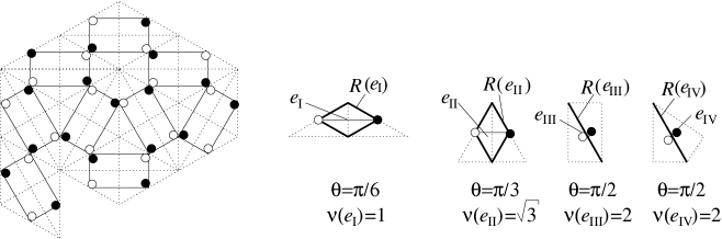
Figure 2: Dual graph of a lozenge-with-diagonals tiling (left). Critical weights for quadri-tiles (right).

2.2 Dirac and inverse Dirac operator

Results in this section are due to Kenyon [18], see also Mercat [25]. Define the Hermitian matrix $K$ indexed by vertices of $G^{*}$ as follows. If $v_{1}$ and $v_{2}$ are not adjacent, $K(v_{1},v_{2})=0$. If $w\in W$ and $b\in B$ are adjacent vertices, then $K(w,b)=\overline{K(b,w)}$ is the complex number of modulus $\nu(wb)$ and direction pointing from $w$ to $b$. Another useful way to say this is as follows. Let $R(wb)$ be the rhombus associated to the edge $wb$, and denote by $w,x,b,y$ its vertices in cclw (counterclockwise) order, then $K(w,b)$ is $i$ times the complex vector $x-y$. If $w$ and $b$ have the same image in the plane, then $|K(w,b)|=2$, and the direction of $K(w,b)$ is that which is perpendicular to the corresponding dual edge, and has sign determined by the local orientation. The infinite matrix $K$ defines the Dirac operator $K$: ${\mathbb{C}}^{V(G^{*})}\rightarrow{\mathbb{C}}^{V(G^{*})}$, by

$$(Kf)(v)=\sum_{u\in G^{*}}K(v,u)f(u),$$

where $V(G^{*})$ denotes the set of vertices of the graph $G^{*}$.
The inverse Dirac operator $K^{-1}$ is defined to be the operator which satisfies

1. $KK^{-1}=\mbox{Id}$,

2. $K^{-1}(b,w)\rightarrow 0$, when $|b-w|\rightarrow\infty$.

In [18], Kenyon proves uniqueness of $K^{-1}$, and existence by giving an explicit expression for $K^{-1}(b,w)$ as a function of the local geometry of the graph.

2.3 Minimal free energy Gibbs measure for isoradial graphs

If $e_{1}=w_{1}b_{1},\ldots,e_{k}=w_{k}b_{k}$ is a subset of edges of $G^{*}$, define the cylinder set $\{e_{1},\ldots,e_{k}\}$ of $G^{*}$ to be the set of dimer configurations of $G^{*}$ which contain the edges $e_{1},\ldots,e_{k}$. Let ${\cal A}$ be the field consisting of the empty set and of the finite disjoint unions of cylinders. Denote by $\sigma({\cal A})$ the $\sigma$-field generated by ${\cal A}$.

Theorem 3

[6] Assume $G^{*}$ is doubly periodic. Then, there is a probability measure $\mu$ on $({\cal M}(G^{*}),\sigma({\cal A}))$ such that for every cylinder $\{e_{1},\ldots,e_{k}\}$ of $G^{*}$,

$$\mu(e_{1},\ldots,e_{k})=\left(\prod_{i=1}^{k}K(w_{i},b_{i})\right)\det_{1\leq i,\;j\leq k}\left(K^{-1}(b_{i},w_{j})\right).$$ (1)

Moreover $\mu$ is a Gibbs measure on ${\cal M}(G^{*})$, and it is the unique Gibbs measure which has minimal free energy per fundamental domain among the two-parameter family of translation invariant, ergodic Gibbs measures of [26].

Remark 4

 
$\bullet$ Refer to [21] for the definition of the free energy per fundamental domain.
$\bullet$ In [6], we prove that the periodicity assumption can be released in the case of lozenge-with-diagonals tilings. That is, given any lozenge-with-diagonals tiling of ${\cal L}$, equation (1) defines a Gibbs measure on dimer configurations of its dual graph. Although fundamental domains make no sense in case of non-periodic graphs, the minimal free energy property can still be interpreted in some wider sense.

2.4 Gibbs measure on triangular quadri-tilings

The construction of this section is taken from [6]. Consider the set ${\cal Q}$ of all triangular quadri-tilings of the plane up to isometry, and assume that quadri-tiles are assigned a positive weight function. Then the notion of Gibbs measure on ${\cal Q}$ is a natural extension of the one used in the case of dimer configurations of fixed graphs. It is a probability measure that satisfies the following: if a triangular quadri-tiling is fixed in an annular region, then triangular quadri-tilings inside and outside of the annulus are independent; moreover, the probability of any interior triangular quadri-tiling is proportional to the product of the weights of the quadri-tiles. Denoting by ${\cal M}$ the set of dimer configurations corresponding to triangular quadri-tilings of ${\cal Q}$, and using the bijection between ${\cal Q}$ and ${\cal M}$, we obtain the definition of a Gibbs measure on ${\cal M}$.
Define ${\cal L}^{*}$ to be set of dual graphs $L^{*}$ of lozenge-with-diagonals tilings $L\in{\cal L}$. Although some edges of ${\cal L}^{*}$ have length $0$, we think of them as edges of the one skeleton of the graphs, so that to every edge of ${\cal L}^{*}$, there corresponds a unique quadri-tile. Let $e$ be an edge of ${\cal L}^{*}$, and let $q_{e}$ be the corresponding quadri-tile, then $q_{e}$ is made of two adjacent right triangles. If the two triangles share the hypotenuse edge, they belong to two adjacent lozenges; else if they share a leg, they belong to the same lozenge. Let us call these lozenge(s) the lozenge(s) associated to the edge $e$, and denote it/them by ${\sf l}_{e}$ (that is ${\sf l}_{e}$ consists of either one or two lozenges). Let ${\sf k}_{e}$ be the edge(s) of ${\mathbb{T}}^{*}$ corresponding to the lozenge(s) ${\sf l}_{e}$. Let us introduce one more definition, if $\{e_{1},\ldots,e_{k}\}$ is a subset of edges of ${\cal L}^{*}$, then the cylinder set $\{e_{1},\ldots,e_{k}\}$ is the set of dimer configurations of ${\cal M}$ which contain these edges. Denote by ${\cal C}$ the field consisting of the empty set and of the finite disjoint unions of cylinders. Denote by $\sigma({\cal C})$ the $\sigma$-field generated by ${\cal C}$.
Consider a lozenge-with-diagonals tiling $L\in{\cal L}$, and denote by $\mu^{L}$ the minimal free energy per fundamental domain Gibbs measure on $({\cal M}(L^{*}),\sigma({\cal A}))$ given by Theorem 3, where $\sigma({\cal A})$ is the $\sigma$-field of cylinders of ${\cal M}(L^{*})$. Similarly, denote by $\mu^{\mathbb{T}}$ the minimal free energy per fundamental domain Gibbs measure on $({\cal M}({\mathbb{T}}^{*}),\sigma({\cal B}))$, where $\sigma({\cal B})$ is the $\sigma$-field of cylinders of ${\cal M}({\mathbb{T}}^{*})$.
Let us define $\tilde{\mu}^{L}$ on $({\cal M},\sigma({\cal C}))$ by:

$$\tilde{\mu}^{L}(e_{1},\ldots,e_{k})=\left\{\begin{array}[]{ll}\mu^{L}(e_{1},\ldots,e_{k})&\mbox{if the lozenges ${\sf l}_{e_{1}},\ldots,{\sf l}_{e_{k}}$ belong to ${\sf L}$},\vspace{0.2cm}\\ 0&\mbox{else},\end{array}\right.$$

where we recall that ${\sf L}$ is the lozenge tiling obtained from the lozenge-with-diagonals tiling $L$ by removing the diagonals. Then, it is easy to check that $\tilde{\mu}^{L}$ is a probability measure on $({\cal M},\sigma({\cal C}))$. In order to simplify notations, we write $\mu^{L}$ for $\tilde{\mu}^{L}$ whenever no confusion occurs.
Now, on $({\cal M}\times{\cal M}({\mathbb{T}}^{*}),{\cal B}\times{\cal C})$, define:

$${\mathbb{P}}((e_{1},\ldots,e_{k})\times(k_{1},\ldots,k_{m}))=\sum_{\{{\sf L}^{*}\in{\cal M}({\mathbb{T}}^{*}):k_{1},\ldots,k_{m}\in{\sf L}^{*}\}}\mu^{L}(e_{1},\ldots,e_{k})d\mu^{\mathbb{T}}({\sf L}^{*}).$$

Using Kolomogorov’s extension theorem, ${\mathbb{P}}$ extends to a probability measure on $({\cal M}\times{\mathbb{T}}^{*},\sigma({\cal B}\times{\cal C}))$. Let us also denote by ${\mathbb{P}}$ the marginal of ${\mathbb{P}}$ on ${\cal M}$, then in [6], ${\mathbb{P}}$ is shown to be a Gibbs measure on ${\cal M}$, and conjectured to be of minimal free energy per fundamental domain among a four-parameter family of translation invariant, ergodic Gibbs measures.

3 Height functions

In the whole of this section, we let $G$ be an isoradial graph whose dual graph $G^{*}$ is bipartite; as before, $B$ denotes the set of black vertices, $W$ the set of white ones. We define the height function $h$ on vertices of $2$-tilings of $G$, whose fluctuations are described in Theorem 1. As in [21], see also [4], $h$ is defined using flows.
The bipartite coloring of the vertices of $G^{*}$ induces an orientation of the faces of $G$: color the dual faces of the black (white) vertices black (white); orient the boundary edges of the black faces cclw, the boundary edges of the white faces are then oriented cw.

3.1 Definition

Let us first define a flow $\omega_{0}$ on the edges of $G^{*}$. Consider an edge $wb$ of $G^{*}$, then $R(wb)$ is the rhombus associated to $wb$, and $\theta_{wb}$ is the corresponding rhombus angle. Define $\omega_{0}$ to be the white-to-black flow, which flows by $\theta_{wb}/\pi$ along every edge $wb$ of $G^{*}$.

Lemma 5

The flow $\omega_{0}$ has divergence $1$ at every white vertex, and $-1$ at every black vertex of $G^{*}$.

Proof:
By definition of the rhombus angle, we have

$$\forall w\in W,\sum_{b:b\sim w}2\theta_{wb}=2\pi;\;\forall b\leavevmode\nobreak{\c{c}}\in\leavevmode\nobreak{\c{c}}B,\sum_{w:w\sim b}2\theta_{wb}=2\pi.$$

$\square$

Now, consider a $2$-tiling $T$ of $G$, and let $M$ be the corresponding perfect matching of $G^{*}$. Then $M$ defines a white-to-black unit flow $\omega$ on the edges of $G^{*}$: flow by $1$ along every edge of $M$, from the white vertex to the black one. The difference $\omega_{0}-\omega$ is a divergence free flow, which means that the quantity of flow that enters any vertex of $G^{*}$ equals the quantity of flow which exists that same vertex.
We are ready for the definition of the height function $h$. Choose a vertex $v_{0}$ of $G$, and fix $h(v_{0})=0$. For every other vertex $v$ of $T$, take an edge-path $\gamma$ of $G$ from $v_{0}$ to $v$. If an edge $uv$ of $\gamma$ is oriented in the direction of the path, and if we denote by $e$ its dual edge, then $h$ increases by $\omega_{0}(e)-\omega(e)$ along $uv$; if an edge $uv$ is oriented in the opposite direction, then $h$ decreases by the same quantity along $uv$. As a consequence of the fact that $\omega_{0}-\omega$ is a divergence free flow, the height function $h$ is well defined.
The following lemma gives a correspondence between height functions defined on vertices of $G$, and $2$-tilings of $G$.

Lemma 6

Let $\tilde{h}$ be an ${\mathbb{R}}$-valued function on vertices of $G$ satisfying

1. $\tilde{h}(v_{0})=0$,

2. $\tilde{h}(v)-\tilde{h}(u)=\omega_{0}(e)$ or $\omega_{0}(e)-1$ for any edge $uv$ oriented from $u$ to $v$, where $e$ denotes the dual edge of $uv$.

Then, there is a bijection between functions $\tilde{h}$ satisfying these two conditions, and $2$-tilings of $G$.

Proof:
The idea of the proof closely follows [8]. Let $T$ be a $2$-tiling of $G$, $M$ be the corresponding matching, and $\omega$ be the unit white-to-black flow defined by $M$. Then, the height function $h$ satisfies the conditions of the lemma: consider an edge $uv$ of $G$ oriented from $u$ to $v$ and denote by $e$ its dual edge, then $h(v)-h(u)=\omega_{0}(e)-\omega(e)$, and by definition $\omega(e)=0$ or $1$.
Conversely, consider an ${\mathbb{R}}$-valued function $\tilde{h}$ as in the lemma. Let us construct a $2$-tiling $T$ whose height function is $\tilde{h}$. Consider a black face $F$ of $G$, and let $e_{1},\ldots,e_{m}$ be the dual edges of its boundary edges. Then $\sum_{i=1}^{m}\omega_{0}(e_{i})=1$, so that there is exactly one boundary edge $uv$ along which $\tilde{h}(v)-\tilde{h}(u)$ is $\omega_{0}(e_{i})-1$ (where $e_{i}$ is the dual edge of $uv$). To the face $F$, we associate the $2$-tile of $G$ which is crossed by the edge $uv$. Repeating this procedure for all black faces of $G$, we obtain $T$. $\square$

3.2 Interpretation

The discrete interface interpretation of $2$-tilings was first given by Thurston in the case of lozenges [30]. Following him, a $2$-tiling of $G$ can be seen as a discrete $2$-dimensional surface $S$ in a $3$-dimensional space that has been projected orthogonally to the plane; the “height” of $S$ is given by the function $h$. Stated in physics terminology, $2$-tilings of $G$ are random interfaces in dimension $2+1$.

3.3 Example: the two height functions of triangular quadri-tilings

Consider a triangular quadri-tiling $T\in{\cal Q}$. Then, recall that $h_{1}$ assigns to vertices of $T$ the “height” of $T$ interpreted as a $2$-tiling of its underlying lozenge-with-diagonals tiling $L(T)$, and $h_{2}$ assigns to vertices of $T$ the “height” of ${\sf L}(T)$ interpreted as a $2$-tiling of ${\mathbb{T}}$. Let us now explicitly compute $h_{1}$ and $h_{2}$.
The definition of the flow $\omega_{0}(L(T))$ on edges of $L(T)^{*}$ uses the rhombus angles of the edges of $L(T)^{*}$. These have been computed in Section 2.1.2 and are equal to $\frac{\pi}{6},\frac{\pi}{3},\frac{\pi}{2}$ for edges of type I, II, III and IV respectively. Hence if $uv$ is the boundary edge of a quadri-tile of $T$, oriented from $u$ to $v$, then the height change of $h_{1}$ along $uv$ is $\frac{1}{6},\frac{1}{3},\frac{1}{2}$ depending on whether the dual edge $e$ of the edge $uv$ is of type I, II, III or IV respectively, see Figure 3.
In a similar way, the flow $\omega_{0}({\mathbb{T}}^{*})$ on edges of ${\mathbb{T}}^{*}$ flows by $\frac{1}{3}$ along every edge, so that if $u^{\prime}v^{\prime}$ be a boundary edge of a lozenge of ${\sf L}(T)$ oriented from $u^{\prime}$ to $v^{\prime}$, then the height change of $h_{2}$ along $u^{\prime}v^{\prime}$ is equal to $\frac{1}{3}$. Thinking of a lozenge as the projection to the plane of the face of a cube [30], there is a natural way to assign a value for $h_{2}$ at the vertex at the crossing of the diagonals of the lozenges, see Figure 3.

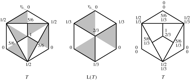
Figure 3: From left to right: triangular quadri-tiling T and first height function $h_{1}$, underlying lozenge tiling ${\sf L}(T)$ and second height function $h_{2}$, T with height functions $h_{1}$ (above) and $h_{2}$ (below).

By means of $h_{1}$ and $h_{2}$, a triangular quadri-tiling $T$ of ${\cal Q}$ is interpreted in [6] as a $2$-dimensional discrete surface $S_{1}$ in a $4$-dimensional space that has been projected orthogonally to the plane. $S_{1}$ can also be projected to $\frac{1}{3}\widetilde{{\mathbb{Z}}}^{3}$ ($\widetilde{{\mathbb{Z}}}^{3}$ is the space ${\mathbb{Z}}^{3}$ where the cubes are drawn with diagonals on their faces), and one obtains a surface $S_{2}$. When projected to the plane $S_{2}$ is the underlying lozenge-with-diagonals tiling $L(T)$. This can be restated by saying that triangular quadri-tilings of ${\cal Q}$ are discrete interfaces in dimension $2+2$.

4 Gaussian free field of the plane

Theorem 1 and Corollary 2 prove convergence of the height function $h$ to a Gaussian free field. The goal of this section is to define the Gaussian free field of the plane. We refer to [9, 27] for other ways of the defining the Gaussian free field.

4.1 The Green function of the plane, and Dirichlet energy

The Green function of the plane, denoted by $g$, is the kernel of the Laplace equation in the plane, it satisfies $\Delta_{x}g(x,y)=\delta_{x}(y)$, where $\delta_{x}$ is the Dirac distribution at $x$. Up to an additive constant, $g$ is given by

$$g(x,y)=-\frac{1}{2\pi}\log|x-y|.$$

Define the following bilinear form

$$\begin{array}[]{rccl}G:&C_{c,0}^{\infty}({\mathbb{R}}^{2})\times C_{c,0}^{\infty}({\mathbb{R}}^{2})&\longrightarrow&{\mathbb{R}}\\ &({\varphi}_{1},{\varphi}_{2})&\longmapsto&G({\varphi}_{1},{\varphi}_{2})=\displaystyle\int_{{\mathbb{R}}^{2}}\int_{{\mathbb{R}}^{2}}g(x,y){\varphi}_{1}(x){\varphi}_{2}(y)dx\,dy.\\ \end{array}$$

$G({\varphi},{\varphi})$ is called the Dirichlet energy of ${\varphi}$. Let us consider the topology induced by the $L^{\infty}$ norm on $C_{c,0}^{\infty}({\mathbb{R}}^{2})$.

Lemma 7

$G$ is a continuous, positive definite, bilinear form.

Proof:
$G$ is continuous

This is a consequence of the fact that for every ${\varphi}_{1},{\varphi}_{2}\in C_{c,0}^{\infty}({\mathbb{R}}^{2})$, the function $g(x,y)$ is integrable.
$G$ is positive definite

For $i=1,2$, denote by $K_{i}=\mbox{supp}({\varphi}_{i})$, and let $f_{i}(x)=\int_{{\mathbb{R}}^{2}}g(x,y){\varphi}_{i}(y)dy$. Let us prove that

$$G({\varphi}_{1},{\varphi}_{2})=\int_{{\mathbb{R}}^{2}}\nabla f_{1}(x).\nabla f_{2}(x)dx.$$ (2)

For any $R>0$, Green’s formula implies

$$\int_{B(0,R)}\nabla f_{1}(x).\nabla f_{2}(x)dx=-\int_{B(0,R)}\triangle f_{1}(x)f_{2}(x)dx+\int_{S(0,R)}f_{2}(x)\nabla f_{1}(x).n(x)ds.$$ (3)

Assume $R$ is large enough so that $K_{1},K_{2}\subset B(0,R)$. The first term of the right hand side of (3) satisfies

$$-\int_{B(0,R)}\triangle f_{1}(x)f_{2}(x)dx = -\int_{B(0,R)}\triangle_{x}\left(\int_{K_{1}}g(x,y){\varphi}_{1}(y)dy\right)\left(\int_{K_{2}}g(x,y){\varphi}_{2}(y)dy\right)dx,$$

$$= \int_{K_{1}}\int_{K_{2}}g(x,y){\varphi}_{1}(x){\varphi}_{2}(y)dy\,dx=G({\varphi}_{1},{\varphi}_{2}).$$

In order to evaluate the second term of the right hand side of (3), let us compute

$$\nabla f_{1}(x).n(x) = -\frac{1}{2\pi}\int_{K_{1}}{\varphi}_{1}(y)\nabla\log|x-y|.n(x)dy,$$

$$= -\frac{1}{2\pi}\int_{K_{1}}{\varphi}_{1}(y)\frac{|x|}{|x-y|^{2}}dy,$$

$$= -\frac{1}{2\pi}\int_{K_{1}}{\varphi}_{1}(y)\left(\frac{|x|}{|x-y|^{2}}-\frac{1}{|x|}\right)dy-\frac{1}{2\pi}\int_{K_{1}}{\varphi}_{1}(y)\frac{1}{|x|}dy,$$

$$= -\frac{1}{2\pi}\int_{K_{1}}{\varphi}_{1}(y)\left(\frac{|x|}{|x-y|^{2}}-\frac{1}{|x|}\right)dy\mbox{ (since ${\varphi}_{1}$ is a mean $0$ function)}.$$

$\forall\,x\in S(0,R)$, $\forall\,y\in K_{1}$, we have $\frac{|x|}{|x-y|^{2}}-\frac{1}{|x|}=O\left(\frac{1}{R^{2}}\right)$, hence $|\nabla f_{1}(x).n(x)|=O\left(\frac{1}{R^{2}}\right)$; $\forall\,x\in S(0,R)$, we also have $|f_{2}(x)|=O(\log R)$, thus the second term of the right hand side of (3) is $O\left(\frac{\log R}{R}\right)$. Taking the limit as $R\rightarrow\infty$ in (3), we obtain (2).

Let us assume $G({\varphi}_{1},{\varphi}_{1})=0$. By equality (2) this is equivalent to $\int_{{\mathbb{R}}^{2}}|\nabla f_{1}(x)|^{2}dx=0$, hence $\nabla f_{1}\equiv(0,0)$. Since ${\varphi}_{1}(x)=\triangle f_{1}(x)=\mbox{div}(\nabla f_{1}(x))$, we deduce ${\varphi}_{1}\equiv 0$. $\square$

4.2 Random distributions

The following definitions are taken from [10]. A random function $F$ associates to every function ${\varphi}\in C_{c,0}^{\infty}({\mathbb{R}}^{2})$ a real random variable $F{\varphi}$. For ${\varphi}_{1},\ldots,{\varphi}_{k}\in C_{c,0}^{\infty}({\mathbb{R}}^{2})$, we suppose that the joint probabilities $a_{n}\leq F{\varphi}_{n}<b_{n}$, $1\leq n\leq k$ are given, and we ask that they satisfy the compatibility relation. A random function $F$ is linear if $\forall\,{\varphi}_{1},{\varphi}_{2}\in C_{c,0}^{\infty}({\mathbb{R}}^{2})$,

$$F(\alpha{\varphi}_{1}+\beta{\varphi}_{2})=\alpha F{\varphi}_{1}+\beta F{\varphi}_{2}.$$

It is continuous if convergence of the functions ${\varphi}_{n_{j}}$ to ${\varphi}_{j}$ $(1\leq j\leq k)$ implies

$$\lim_{n\rightarrow\infty}(F{\varphi}_{n_{1}},\ldots,F{\varphi}_{n_{k}})=(F{\varphi}_{1},\ldots,F{\varphi}_{k}),$$

that is, if $P(x)$ (resp. $P_{n}(x)$) is the probability measure corresponding to the random variable $(F{\varphi}_{1},\ldots,F{\varphi}_{k})$ (resp. $(F{\varphi}_{n_{1}},\ldots,F{\varphi}_{n_{k}})$), then for any bounded continuous function $f$

$$\lim_{n\rightarrow\infty}\int f(x_{1},\ldots,x_{k})dP_{n}(x)=\int f(x_{1},\ldots,x_{k})dP(x).$$

A random distribution $F$ is a random function which is linear and continuous. It is said to be Gaussian if for every linearly independent functions ${\varphi}_{1},\ldots,{\varphi}_{k}\in C_{c,0}^{\infty}({\mathbb{R}}^{2})$, the random vector $(F{\varphi}_{1},\ldots,F{\varphi}_{k})$ is Gaussian.

Two random distributions $F$ and $G$ are said to be independent if for any functions ${\varphi}_{1},\ldots,{\varphi}_{k}\in C_{c,0}^{\infty}({\mathbb{R}}^{2})$, the random vectors $(F{\varphi}_{1},\ldots,F{\varphi}_{k})$ and $(G{\varphi}_{1},\ldots,G{\varphi}_{k})$ are independent.

4.3 Gaussian free field of the plane

Theorem 8

[3] If $G:C_{c,0}^{\infty}({\mathbb{R}}^{2})\times C_{c,0}^{\infty}({\mathbb{R}}^{2})\rightarrow{\mathbb{R}}$ is a bilinear, continuous, positive definite form, then there exists a Gaussian random distribution $F$, whose covariance function is given by

$${\mathbb{E}}(F{\varphi}_{1}F{\varphi}_{2})=G({\varphi}_{1},{\varphi}_{2}).$$

Using Lemma 7, and Theorem 8, we define a Gaussian free field of the plane to be a Gaussian random distribution whose covariance function is

$${\mathbb{E}}(F{\varphi}_{1}F{\varphi}_{2})=-\frac{1}{2\pi}\int_{{\mathbb{R}}^{2}}\int_{{\mathbb{R}}^{2}}\log|x-y|{\varphi}_{1}(x){\varphi}_{2}(y)\,dx\,dy.$$

5 Proof of Theorem 1

We place ourselves in the context of Theorem 1: $G$ is an isoradial graph whose dual graph $G^{*}$ is doubly periodic and bipartite; edges of $G^{*}$ are assigned the critical weight function, and $G^{\varepsilon}$ is the graph $G$ whose edge-lengths have been multiplied by ${\varepsilon}$. Recall the following notations: $H^{\varepsilon}{\varphi}={\varepsilon}^{2}\sum_{v\in V(G^{\varepsilon})}a(v^{*}){\varphi}(v)h^{\varepsilon}(v)$, $\mu$ is the minimal free energy per fundamental domain Gibbs measure for the dimer model on $G^{*}$ of Section 2.3, and $F$ is a Gaussian free field of the plane.
Since the random vector $(F{\varphi}_{1},\ldots,F{\varphi}_{k})$ is Gaussian, to prove convergence of $(H^{\varepsilon}{\varphi}_{1},\\ \ldots,H^{\varepsilon}{\varphi}_{k})$ to $(F{\varphi}_{1},\ldots,F{\varphi}_{k})$, it suffices to prove convergence of the moments of $(H^{\varepsilon}{\varphi}_{1},\ldots,$$H^{\varepsilon}{\varphi}_{k})$ to those of $(F{\varphi}_{1},\ldots,F{\varphi}_{k})$; that is we need to show that for every $k$-tuple of positive integers $(m_{1},\ldots,m_{k})$, we have

$$\lim_{{\varepsilon}\rightarrow 0}{\mathbb{E}}[(H^{\varepsilon}{\varphi}_{1})^{m_{1}}\ldots(H^{\varepsilon}{\varphi}_{k})^{m_{k}}]={\mathbb{E}}[(F{\varphi}_{1})^{m_{1}}\ldots(F{\varphi}_{k})^{m_{k}}].$$ (4)

In Section 5.1, we prove two properties of the height function $h$, and in Section 5.2, we give the asymptotic formula of [18] for the inverse Dirac operator $K^{-1}$. Using these results in Section 5.3, we prove a formula for the limit (as ${\varepsilon}\rightarrow 0$) of the $k^{\mbox{{\scriptsize th}}}$ moment of $h$. This allows us to show convergence of ${\mathbb{E}}[(H^{\varepsilon}{\varphi})^{k}]$ to ${\mathbb{E}}[(F{\varphi})^{k}]$ in Section 5.4. One then obtains equation (4) by choosing ${\varphi}$ to be a suitable linear combination of the ${\varphi}_{i}$’s.
As before, $B$ denotes the set of black vertices of $G^{*}$, and $W$ the set of white ones. Moreover, we suppose that faces of $G$ have the orientation induced by the bipartite coloring of the vertices of $G^{*}$.

5.1 Properties of the height function

Let $u,\,v$ be two vertices of $G$, and let $\gamma$ be an edge-path of $G$ from $u$ to $v$. First, consider edges of $\gamma$ which are oriented in the direction of the path, that is edges which have a black face of $G$ on the left, and denote by $f_{1},\ldots,f_{n}$ their dual edges. Hence an edge $f_{j}$ consists of a black vertex on the left of $\gamma$, and of a white one on the right. Similarly, consider edges of $\gamma$ which are oriented in the opposite direction, and denote by $e_{1},\ldots,e_{m}$ their dual edges, hence an edge $e_{i}$ consists of a white vertex on the left of $\gamma$, and of a black one on the right. Let ${\mathbb{I}}_{e}$ be the indicator function of ${\cal M}(G^{*})$: ${\mathbb{I}}_{e}(M)=1$, if the edge $e$ belongs to the dimer configuration $M$ of $G^{*}$, and $0$ else.

Lemma 9

$$h(v)-h(u)=\sum_{j=1}^{m}({\mathbb{I}}_{e_{j}}-\mu(e_{j}))+\sum_{j=1}^{n}(-{\mathbb{I}}_{f_{j}}+\mu(f_{j})).$$

Proof:
Let $e_{j}$ be the dual edge of an edge $u_{j}v_{j}$ of $\gamma$ oriented from $v_{j}$ to $u_{j}$. Denote by $\theta_{j}$ the rhombus angle of the edge $e_{j}$, then by Lemma 6,

$$h(v_{j})-h(u_{j})=\left\{\begin{array}[]{ll}-\frac{\theta_{j}}{\pi}+1&\mbox{if the edge $e_{j}$ belongs to the dimer configuration of $G^{*}$},\vspace{0.2cm}\\ -\frac{\theta_{j}}{\pi}&\mbox{else}.\end{array}\right.$$

Hence $h(v_{j})-h(u_{j})=(-\frac{\theta_{j}}{\pi}+1){\mathbb{I}}_{e_{j}}-\frac{\theta_{j}}{\pi}(1-{\mathbb{I}}_{e_{j}})={\mathbb{I}}_{e_{j}}-\frac{\theta_{j}}{\pi}$. Moreover, a direct computation using formula (1) yields $\mu(e_{j})=\theta_{j}/\pi$, so

$$h(v_{j})-h(u_{j})={\mathbb{I}}_{e_{j}}-\mu(e_{j}).$$

Similarly, when $f_{j}$ is the dual edge of an edge $u_{j}^{\prime}v_{j}^{\prime}$ of $\gamma$ oriented from $u_{j}^{\prime}$ to $v_{j}^{\prime}$, we obtain $h(v_{j}^{\prime})-h(u_{j}^{\prime})=-{\mathbb{I}}_{f_{j}}+\mu(f_{j})$, and we conclude

$$h(v)-h(u)=\sum_{j=1}^{m}h(v_{j})-h(u_{j})+\sum_{j=1}^{n}h(v_{j}^{\prime})-h(u_{j}^{\prime})=\sum_{j=1}^{m}({\mathbb{I}}_{e_{j}}-\mu(e_{j}))+\sum_{j=1}^{n}(-{\mathbb{I}}_{f_{j}}+\mu(f_{j})).$$

$\square$

Lemma 10

$${\mathbb{E}}_{\mu}[h(v)-h(u)]=0.$$

Proof:
By Lemma 9 we have, $\displaystyle{\mathbb{E}}_{\mu}[h(v)-h(u)]=\sum_{j=1}^{m}{\mathbb{E}}_{\mu}[{\mathbb{I}}_{e_{j}}-{\mu}(e_{j})]+\sum_{j=1}^{n}{\mathbb{E}}_{\mu}[-{\mathbb{I}}_{f_{j}}+{\mu}(f_{j})]=0.$ $\square$

5.2 Asymptotics of the inverse Dirac operator $K^{-1}$

In order to state the asymptotic formula of [18] for the inverse of the Dirac operator $K$ indexed by vertices of $G^{*}$, we let $w\in W$ be a white vertex of $G^{*}$, $v$ any other vertex of $G^{*}$, and define the rational function $f_{wv}(z)$ of [18]. Recall that $\widetilde{R}$ is the set of rhombi associated to edges of $G^{*}$, and consider $w=v_{0},v_{1},v_{2},\ldots,v_{k}=v$ an edge-path of $\widetilde{R}$ from $w$ to $v$. Each edge $v_{j}v_{j+1}$ has exactly one vertex of $G^{*}$ (the other is a vertex of $G$). Direct the edge away from this vertex if it is white, and towards this vertex if it is black. Let $e^{i\alpha_{j}}$ be the corresponding vector in $\widetilde{R}$ (which may point contrary to the direction of the path). Then, $f_{wv}$ is defined inductively along the path, starting from

$$f_{ww}(0)=1.$$

If the edge leads away from a white vertex, or towards a black vertex, then

$$f_{wv_{j+1}}(z)=\frac{f_{wv_{j}}(z)}{1-e^{i\alpha_{j}}},$$

else, if it leads towards a white vertex, or away from a black vertex, then

$$f_{wv_{j+1}}(0)=f_{wv_{j}}(z).(z-e^{i\alpha_{j}}).$$

The function $f_{wv}(z)$ is well defined (i.e. independent of the edge-path of $\widetilde{R}$ from $w$ to $v$). Then, Kenyon gives the following asymptotics for the inverse Dirac operator $K^{-1}$:

Theorem 11

[18] Asymptotically, as $|b-w|\rightarrow\infty$,

$$K^{-1}(b,w)=\frac{1}{2\pi}\left(\frac{1}{b-w}+\frac{f_{wb}(0)}{\bar{b}-\bar{w}}\right)+O\left(\frac{1}{|b-w|^{2}}\right).$$

5.3 Moment formula

Let $u_{1},\ldots,u_{k},v_{1},\ldots,v_{k}$ be distinct points of ${\mathbb{R}}^{2}$, and let $\gamma_{1},\ldots,\gamma_{k}$ be pairwise disjoint paths such that $\gamma_{j}$ runs from $u_{j}$ to $v_{j}$. Let $u_{j}^{{\varepsilon}},v_{j}^{{\varepsilon}}$ be vertices of ${G^{\varepsilon}}$ lying within $O({\varepsilon})$ of $u_{j}$ and $v_{j}$ respectively. In order to simplify notations, we write $h$ for the unnormalized height function $h^{\varepsilon}$ on $2$-tilings of $G^{\varepsilon}$. Then, we have

Proposition 12

For every $k\in{\mathbb{N}}$, $k\geq 2$

$$\lim_{{\varepsilon}\rightarrow 0}{\mathbb{E}}[(h(v_{1}^{{\varepsilon}})-h(u_{1}^{{\varepsilon}}))\ldots(h(v_{k}^{{\varepsilon}})-h(u_{k}^{{\varepsilon}}))]=\\ \frac{(-i)^{k}}{(2\pi)^{k}}\sum_{{\varepsilon}=0,1}(-1)^{k{\varepsilon}}\left(\int_{\gamma_{1}}\ldots\int_{\gamma_{k}}\det_{\begin{array}[]{l}\scriptstyle i,j\in[1,k]\\ \scriptstyle i\neq j\end{array}}\left(\frac{1}{z_{i}^{\varepsilon}-z_{j}^{\varepsilon}}\right)dz_{1}^{\varepsilon}\ldots dz_{k}^{\varepsilon}\right),$$ (5)

where $z_{i}^{0}=z_{i}$ and $z_{i}^{1}=\bar{z_{i}}$.

Proof:
Steps of the proof follow [16], but since we work in a much more general setting, they are adapted in a non-trivial way.
Let $\gamma_{1}^{{\varepsilon}},\ldots,\gamma_{k}^{{\varepsilon}}$ be pairwise disjoint paths of ${G^{\varepsilon}}$, such that $\gamma_{j}^{{\varepsilon}}$ runs from $u_{j}^{{\varepsilon}}$ to $v_{j}^{{\varepsilon}}$ and approximates $\gamma_{j}$ within $O({\varepsilon})$. For every $j$, denote by $f_{js}$ the dual edge of the $s^{\mbox{{\scriptsize th}}}$ edge of the path $\gamma_{j}^{\varepsilon}$, which is oriented in the direction of the path: $f_{js}$ consists of a black vertex on the left of $\gamma_{j}^{{\varepsilon}}$, and of a white one on the right. Denote by $e_{jt}$ the dual edge of the $t^{\mbox{{\scriptsize th}}}$ edge of the path $\gamma_{j}^{\varepsilon}$, which is oriented in the opposite direction: $e_{jt}$ consists of a black vertex on the right of $\gamma_{j}^{{\varepsilon}}$, and of a white one on the left. Using Lemma 9, we obtain
${\mathbb{E}}[(h(v_{1}^{{\varepsilon}})-h(u_{1}^{{\varepsilon}}))\ldots(h(v_{k}^{{\varepsilon}})-h(u_{k}^{{\varepsilon}}))]=$

$$= {\mathbb{E}}\left[\sum_{t_{1}}({\mathbb{I}}_{e_{1t_{1}}}-{\mu}(e_{1t_{1}}))-\sum_{s_{1}}({\mathbb{I}}_{f_{1s_{1}}}-{\mu}(f_{1s_{1}}))\right]\ldots\left[\sum_{t_{k}}({\mathbb{I}}_{e_{kt_{k}}}-{\mu}(e_{kt_{k}}))-\sum_{s_{k}}({\mathbb{I}}_{f_{ks_{k}}}-{\mu}(f_{ks_{k}}))\right],$$ (6)

$$= \sum_{t_{1},\ldots,t_{k}}{\mathbb{E}}[{\mathbb{I}}_{e_{1t_{1}}}-{\mu}(e_{1t_{1}})]\ldots[{\mathbb{I}}_{e_{kt_{k}}}-{\mu}(e_{kt_{k}})]-\ldots+(-1)^{k}\sum_{s_{1},\ldots,s_{k}}{\mathbb{E}}[{\mathbb{I}}_{f_{1s_{1}}}-{\mu}(f_{1s_{1}})]\ldots[{\mathbb{I}}_{f_{ks_{k}}}-{\mu}(f_{ks_{k}})],$$

$$= \sum_{\delta_{1},\ldots,\delta_{k}\in\{0,1\}}\sum_{t_{1}^{\delta_{1}},\ldots,t_{k}^{\delta_{k}}}(-1)^{\delta_{1}+\ldots+\delta_{k}}{\mathbb{E}}[{\mathbb{I}}_{e_{1t_{1}^{\delta_{1}}}}-{\mu}(e_{1t_{1}^{\delta_{1}}})]\ldots[{\mathbb{I}}_{e_{kt_{k}^{\delta_{k}}}}-{\mu}(e_{kt_{k}^{\delta_{k}}})],$$

where $t_{j}^{\delta_{j}}=\left\{\begin{array}[]{l}t_{j}\mbox{ if }\delta_{j}=0\\ s_{j}\mbox{ if }\delta_{j}=1\end{array}\right.,\,e_{jt_{j}^{\delta_{j}}}=e_{jt_{j}^{\delta_{j}}}^{\delta_{j}}=\left\{\begin{array}[]{l}e_{jt_{j}}\mbox{ if }\delta_{j}=0\\ f_{js_{j}}\mbox{ if }\delta_{j}=1\end{array}\right..$
For the time being, let us drop the second subscript. Write $e_{j}=w_{j}b_{j}$ and $f_{j}=w_{j}^{\prime}b_{j}^{\prime}$. Moreover, let us introduce the notation $w_{j}^{\delta_{j}}$, where $w_{j}^{\delta_{j}}=w_{j}$ if $\delta_{j}=0$, and $w_{j}^{\delta_{j}}=w_{j}^{\prime}$ if $\delta_{j}=1$, similarly we introduce the notation $b_{j}^{\delta_{j}}$. Hence we can write a generic term of (6) as

$$(-1)^{\delta_{1}+\ldots+\delta_{k}}{\mathbb{E}}[({\mathbb{I}}_{w_{1}^{\delta_{1}}b_{1}^{\delta_{1}}}-{\mu}(w_{1}^{\delta_{1}}b_{1}^{\delta_{1}}))\ldots({\mathbb{I}}_{w_{k}^{\delta_{k}}b_{k}^{\delta_{k}}}-{\mu}(w_{k}^{\delta_{k}}b_{k}^{\delta_{k}}))].$$

Lemma 13

[13]

$$\begin{split}&(-1)^{\delta_{1}+\ldots+\delta_{k}}{\mathbb{E}}[({\mathbb{I}}_{w_{1}^{\delta_{1}}b_{1}^{\delta_{1}}}-{\mu}(w_{1}^{\delta_{1}}b_{1}^{\delta_{1}}))\ldots({\mathbb{I}}_{w_{k}^{\delta_{k}}b_{k}^{\delta_{k}}}-{\mu}(w_{k}^{\delta_{k}}b_{k}^{\delta_{k}}))]=\\ &=(-1)^{\delta_{1}+\ldots+\delta_{k}}a_{E}\left|\begin{array}[]{cccc}0&K^{-1}(b_{1}^{\delta_{1}},w_{2}^{\delta_{2}})&\dots&K^{-1}(b_{1}^{\delta_{1}},w_{k}^{\delta_{k}})\\ K^{-1}(b_{2}^{\delta_{2}},w_{1}^{\delta_{1}})&0&&\vdots\\ \vdots&&&K^{-1}(b_{k-1}^{\delta_{k-1}},w_{k}^{\delta_{k}})\\ K^{-1}(b_{k}^{\delta_{k}},w_{1}^{\delta_{1}})&\dots&K^{-1}(b_{k}^{\delta_{k}},w_{k-1}^{\delta_{k-1}})&0\end{array}\right|,\end{split}$$ (7)

where $\displaystyle a_{E}=\prod_{j=1}^{k}K(w_{j}^{\delta_{j}},b_{j}^{\delta_{j}})$, and $K$ is the Dirac operator indexed by vertices of $G^{*}$.

A typical term in the expansion of (7) is

$$(-1)^{\delta_{1}+\ldots+\delta_{k}}a_{E}\mbox{ {\rm sgn}}\,\sigma K^{-1}(b_{1}^{\delta_{1}},w_{\sigma(1)}^{\delta_{\sigma(1)}})\ldots K^{-1}(b_{k}^{\delta_{k}},w_{\sigma(k)}^{\delta_{\sigma(k)}}),$$ (8)

where $\sigma\in\widetilde{S_{k}}$, and $\widetilde{S_{k}}$ is the set of permutations of $k$ elements, with no fixed points. To simplify notations, let us assume $\sigma$ is a $k$-cycle, hence (8) becomes

$$(-1)^{\delta_{1}+\ldots+\delta_{k}}a_{E}\mbox{ {\rm sgn}}\,\sigma K^{-1}(b_{1}^{\delta_{1}},w_{2}^{\delta_{2}})\ldots K^{-1}(b_{k}^{\delta_{k}},w_{1}^{\delta_{1}}).$$ (9)

Lemma 14

When ${\varepsilon}$ is small, and for every $\delta_{1},\ldots,\delta_{k}\in\{0,1\}$,

$${\varepsilon}^{k}a_{E}=(-i)^{k}(-1)^{\delta_{1}+\ldots+\delta_{k}}dz_{1}^{\delta_{1}}\ldots dz_{k}^{\delta_{k}}.$$ (10)

Proof:
Let $u_{j}v_{j}$ be an edge of the path $\gamma_{j}^{\varepsilon}$ where $u_{j}$ precedes $v_{j}$. We can write

$$u_{j}v_{j}={\varepsilon}{\ell}(u_{j}v_{j})e^{i\theta_{j}},$$ (11)

where ${\ell}(u_{j}v_{j})$ is the length of the edge $u_{j}v_{j}$ in $G$, and $\theta_{j}$ is the direction from $u_{j}$ to $v_{j}$. Let us first consider the case of an edge $u_{j}v_{j}$ oriented in the direction of the path, that is the dual edge $w_{j}^{\prime}b_{j}^{\prime}$ of $u_{j}v_{j}$ has its black vertex on the left of $\gamma_{j}^{\varepsilon}$. By definition of the Dirac operator, we have $K(w_{j}^{\prime},b_{j}^{\prime})={\ell}(u_{j}v_{j})e^{i\theta_{j}}e^{i\frac{\pi}{2}}$. Next we consider the case of an edge $u_{j}v_{j}$ oriented in the opposite direction, that is its dual edge $w_{j}b_{j}$ has its black vertex on the right of $\gamma_{j}^{\varepsilon}$. Again, using the definition of the Dirac operator, we obtain $K(w_{j},b_{j})={\ell}(u_{j}v_{j})e^{i\theta_{j}}e^{-i\frac{\pi}{2}}$. We summarize the two cases by the following equation

$$K(w_{j}^{\delta_{j}},b_{j}^{\delta_{j}})=(-i)(-1)^{\delta_{j}}{\ell}(u_{j}v_{j})e^{i\theta_{j}}.$$ (12)

When ${\varepsilon}$ is small we replace $u_{j}v_{j}$ by $dz_{j}^{\delta_{j}}$. Thus combining equations (11) and (12) we obtain equation (10). $\square$

Lemma 15

When ${\varepsilon}$ is small and up to a term of order $O({\varepsilon})$, equation $(\ref{525})$ equals

$$\frac{(-i)^{k}}{(2\pi)^{k}}\sum_{{\varepsilon}_{1},\dots,{\varepsilon}_{k}\in\{0,1\}}[f_{w_{2}^{\delta_{2}}b_{1}^{\delta_{1}}}(0)]^{{\varepsilon}_{1}}\ldots[f_{w_{1}^{\delta_{1}}b_{k}^{\delta_{k}}}(0)]^{{\varepsilon}_{k}}F_{{\varepsilon}_{1}}(b_{1}^{\delta_{1}},w_{2}^{\delta_{2}})\ldots F_{{\varepsilon}_{k}}(b_{k}^{\delta_{k}},w_{1}^{\delta_{1}})dz_{1}^{\delta^{1}}\ldots dz_{k}^{\delta^{k}},$$ (13)

where $\displaystyle F_{0}(z,w)=\frac{1}{z-w},\,F_{1}(z,w)={F_{0}(\bar{z},\bar{w})}$, and the functions $f_{wb}$ are defined in Section 5.2.

Proof:
Let us drop the superscripts $\delta_{i}$. Plugging relation (10) in (9), we obtain

$$(\ref{525})=(-i)^{k}\mbox{sgn}\,\sigma K^{-1}(b_{1},w_{2})\ldots K^{-1}(b_{k},w_{1})\frac{1}{{\varepsilon}^{k}}dz_{1}\ldots dz_{k}.$$ (14)

Moreover, for every $i\neq j$, $\displaystyle\lim_{{\varepsilon}\rightarrow 0}\frac{|b_{i}-w_{j}|}{{\varepsilon}}=\infty$, so that by Theorem 11 we have

$$K^{-1}(b_{i},w_{j})=\frac{{\varepsilon}}{2\pi}(F_{0}(b_{i},w_{j})+f_{w_{j}b_{i}}(0)F_{1}(b_{i},w_{j}))+O({\varepsilon}^{2}).$$ (15)

Equation (13) is then (14) where the elements $K^{-1}(b_{i},w_{j})$ have been replaced by (15) and expanded out. $\square$

In what follows, all that we say is true whether the edge $w_{j}^{\delta_{j}}b_{j}^{\delta_{j}}$ has its black vertex on the right or on the left of the path $\gamma_{j}^{\varepsilon}$, that is whether $\delta_{j}=0$ or $1$. So to simplify notations, let us write $\{t_{j}\}$ instead of $\{\delta_{j}\in\{0,1\},t_{j}^{\delta_{j}}\}$, hence $\{t_{j}\}$ is the set of indices which run along the path $\gamma_{j}^{\varepsilon}$. Keeping in mind that our aim is to take the limit as ${\varepsilon}\rightarrow 0$, we replace the vertices $b_{j}$ and $w_{j}$ in the argument of the function $F_{{\varepsilon}_{j}}$ by one common vertex denoted by $z_{j}$. Define
$H({\varepsilon}_{1},\ldots,{\varepsilon}_{k})$=

$$=\sum_{t_{1},\ldots,t_{k}}[f_{w_{2t_{2}}b_{1t_{1}}}(0)]^{{\varepsilon}_{1}}\ldots[f_{w_{1t_{1}}b_{kt_{k}}}(0)]^{{\varepsilon}_{k}}F_{{\varepsilon}_{1}}(z_{1t_{1}},z_{2t_{2}})\ldots F_{{\varepsilon}_{k}}(z_{kt_{k}},z_{1t_{1}})dz_{1t_{1}}\ldots dz_{kt_{k}}.$$

Lemma 16

ç

1.

If $({\varepsilon}_{1},\ldots,{\varepsilon}_{k})=(0,\ldots,0)$, then

$$\lim_{{\varepsilon}\rightarrow 0}H(0,\ldots,0)=\int_{\gamma_{1}}\ldots\int_{\gamma_{k}}F_{0}(z_{1},z_{2})\ldots F_{0}(z_{k},z_{1})dz_{1}\ldots dz_{k}.$$

2.

If $({\varepsilon}_{1},\ldots,{\varepsilon}_{k})=(1,\ldots,1)$, then

$$\lim_{{\varepsilon}\rightarrow 0}H(1,\ldots,1)=(-1)^{k}\int_{\gamma_{1}}\ldots\int_{\gamma_{k}}F_{0}(\bar{z}_{1},\bar{z}_{2})\ldots F_{0}(\bar{z}_{k},\bar{z}_{1})d\bar{z}_{1}\ldots d\bar{z}_{k}.$$

3.

Assume there exists $i\neq j\in\{1,\ldots,k\}$ such that ${\varepsilon}_{i}=0,\,{\varepsilon}_{j}=1$, then

$$\lim_{{\varepsilon}\rightarrow 0}|H({\varepsilon}_{1},\ldots,{\varepsilon}_{k})|=0.$$

Proof:
Here are some preliminary notations. Dropping the second subscript, we consider an edge $u_{j}v_{j}$ of one of the paths $\gamma_{i}^{\varepsilon}$, where $u_{j}$ precedes $v_{j}$. Let us denote by $w_{j}b_{j}$ the dual edge of the edge $u_{j}v_{j}$, and let ${\varepsilon}e^{i\alpha_{j}}=v_{j}-w_{j}$, ${\varepsilon}e^{i\beta_{j}}=b_{j}-v_{j}$. With these notations, we have $dz_{j}={\varepsilon}(e^{i\alpha_{j}}-e^{i\beta_{j}})$ (see Figure 4).

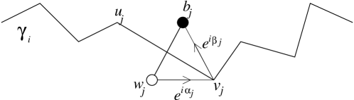
Figure 4: Notations.

Moreover, define

$$J({\varepsilon}_{1},\ldots,{\varepsilon}_{k})=[f_{w_{2}b_{1}}(0)]^{{\varepsilon}_{1}}\ldots[f_{w_{1}b_{k}}(0)]^{{\varepsilon}_{k}}dz_{1}\ldots dz_{k}.$$

Proof of $1.$

$$J(0,\ldots,0)=dz_{1}\ldots dz_{k},$$

so that

$$H(0,\ldots,0)=\sum_{t_{1},\ldots,t_{k}}F_{0}(z_{1t_{1}},z_{2t_{2}})\ldots F_{0}(z_{kt_{k}},z_{1t_{1}})dz_{1t_{1}}\ldots dz_{kt_{k}}.$$

Since the paths $\gamma_{j}$ are disjoint, the function $F_{0}(z_{1},z_{2})\ldots F_{0}(z_{k},z_{1})$ is integrable, and taking the limit as ${\varepsilon}\rightarrow 0$, we obtain $1$.

Proof of $2.$

$$J(1,\ldots,1)=f_{w_{2}b_{1}}(0)\ldots f_{w_{1}b_{k}}(0)\,dz_{1}\ldots dz_{k}.$$

Fix a vertex $v$ of $G^{*}$. Then, by definition of the function $f_{wv}$,

$$J(1,\ldots,1) = f_{w_{2}v}(0)f_{vb_{1}}(0)\ldots f_{w_{1}v}(0)f_{vb_{k}}(0)\,dz_{1}\ldots dz_{k},$$

$$= f_{w_{1}v}(0)f_{vb_{1}}(0)\ldots f_{w_{k}v}(0)f_{vb_{k}}(0)\,dz_{1}\ldots dz_{k},$$

$$= f_{w_{1}b_{1}}(0)\ldots f_{w_{k}b_{k}}(0)\,dz_{1}\ldots dz_{k}.$$

For every $j$, we have $f_{w_{j}b_{j}}(0)=e^{-i(\beta_{j}+\alpha_{j})}$. Moreover, recall that $dz_{j}={\varepsilon}(e^{i\alpha_{j}}-e^{i\beta_{j}})$, so that $-d\bar{z}_{j}=e^{-i(\beta_{j}+\alpha_{j})}dz_{j}$, and we deduce

$$J(1,\ldots,1)=(-1)^{k}d\bar{z}_{1}\ldots d\bar{z}_{k}.$$

This implies,

$$H(1,\ldots,1)=(-1)^{k}\sum_{t_{1},\ldots,t_{k}}F_{0}(\bar{z}_{1t_{1}},\bar{z}_{2t_{2}})\ldots F_{0}(\bar{z}_{kt_{k}},\bar{z}_{1t_{1}})d\bar{z}_{1t_{1}}\ldots d\bar{z}_{kt_{k}}.$$

Taking the limit as ${\varepsilon}\rightarrow 0$, we obtain $2$.

Proof of $3.$

Consider $0<{\ell}<k$, and assume ${\varepsilon}_{1}=\ldots={\varepsilon}_{{\ell}-1}=0$, ${\varepsilon}_{\ell}=\ldots={\varepsilon}_{k}=1$. Let us prove that $\lim_{{\varepsilon}\rightarrow 0}|H(0,\ldots,0,1,\ldots,1)|=0.$ Note that up to a permutation of indices, the argument is the same for the other cases.

$$J(0,\ldots,0,1,\ldots,1)=f_{w_{{\ell}+1}b_{\ell}}(0)\ldots f_{w_{1}b_{k}}(0)\,dz_{1}\ldots dz_{k}.$$

As above, let $v$ be a vertex of $G^{*}$. Then,

$$J(0,\ldots,0,1,\ldots,1)=(f_{vb_{\ell}}(0)dz_{\ell})(f_{w_{1}v}(0)dz_{1})dz_{2}\ldots dz_{{\ell}-1}d\bar{z}_{{\ell}+1}\ldots d\bar{z}_{k}.$$

Introducing the following notation

$$H_{1} = F(z_{2t_{2}},z_{3t_{3}})\ldots F(z_{{{\ell}-2}t_{{\ell}-2}},z_{{{\ell}-1}t_{{\ell}-1}})F(\bar{z}_{{{\ell}+1}t_{{\ell}+1}},\bar{z}_{{{\ell}+2}t_{{\ell}+2}})\ldots F(\bar{z}_{{k-1}t_{k-1}},\bar{z}_{kt_{k}}),$$

$$H_{2} = F(z_{1t_{1}},z_{2t_{2}})F(\bar{z}_{kt_{k}},\bar{z}_{1t_{1}}),$$

$$H_{3} = F(z_{{{\ell}-1}t_{{\ell}-1}},z_{{\ell}t_{\ell}})F(\bar{z}_{{\ell}t_{\ell}},\bar{z}_{{\ell}+1t_{{\ell}+1}}),$$

we obtain $H(0,\ldots,0,1,\ldots,1)=$

$$=\sum_{t_{2},\ldots,\hat{t_{\ell}},\ldots,t_{k}}H_{1}\left(\sum_{t_{1}}H_{2}f_{w_{1t_{1}}v}(0)dz_{1t_{1}}\right)\left(\sum_{t_{\ell}}H_{3}f_{vb_{{\ell}t_{\ell}}}(0)dz_{{\ell}t_{\ell}}\right)dz_{2t_{2}}\ldots dz_{{\ell}-1t_{{\ell}-1}}d\bar{z}_{{\ell}+1t_{{\ell}+1}}\ldots d\bar{z}_{kt_{k}}.\\$$

Let us prove

$$\sum_{t_{\ell}}f_{vb_{{\ell}t_{\ell}}}(0)dz_{{\ell}t_{\ell}}=O({\varepsilon}).$$ (16)

Dropping the second subscript, let $u_{1},v_{1}=u_{2},v_{2}=u_{3},\ldots,v_{m-1}=u_{m},v_{m}$ be the edge-path $\gamma_{\ell}^{\varepsilon}$. Denote by $\xi$ the quantity $f_{vu_{1}}(0)$, then

$$f_{vb_{j}}(0)=\xi e^{i(\beta_{1}-\alpha_{1})}\ldots e^{i(\beta_{j-1}-\alpha_{j-1})}e^{-i\alpha_{j}}.$$

Since $dz_{j}={\varepsilon}(e^{i\alpha_{j}}-e^{i\beta_{j}})$, we obtain

$$f_{vb_{j}}(0)dz_{j}={\varepsilon}\xi\left[\left(e^{i(\beta_{1}-\alpha_{1})}\ldots e^{i(\beta_{j-1}-\alpha_{j-1})}\right)-\left(e^{i(\beta_{1}-\alpha_{1})}\ldots e^{i(\beta_{j-1}-\alpha_{j-1})}e^{i(\beta_{j}-\alpha_{j})}\right)\right],$$

hence

$$\sum_{t_{\ell}}f_{vb_{{\ell}t_{\ell}}}(0)dz_{{\ell}t_{\ell}} = \sum_{j=1}^{m}f_{vb_{j}}(0)dz_{j},$$

$$= {\varepsilon}\xi[1-e^{i(\beta_{1}-\alpha_{1})}+\sum_{j=2}^{m}e^{i(\beta_{1}-\alpha_{1})}\ldots e^{i(\beta_{j-1}-\alpha_{j-1})})-(e^{i(\beta_{1}-\alpha_{1})}\ldots e^{i(\beta_{j-1}-\alpha_{j-1})}e^{i(\beta_{j}-\alpha_{j}})],$$

$$= {\varepsilon}\xi[1-(e^{i(\beta_{1}-\alpha_{1})}\ldots e^{i(\beta_{m}-\alpha_{m})}],\mbox{ (telescopic sum).}$$

We deduce $|\sum_{t_{\ell}}f_{vb_{{\ell}t_{\ell}}}(0)dz_{{\ell}t_{\ell}}|\leq 2{\varepsilon}$, and (16) is proved.
In a similar way we prove $\sum_{t_{1}}f_{w_{1t_{1}}v}(0)dz_{1t_{1}}=O({\varepsilon})$.
Using Taylor expansion in ${\varepsilon}$ for $H_{2}$ and $H_{3}$, we deduce that $\left(\sum_{t_{1}}H_{2}f_{w_{1t_{1}}v}(0)dz_{1t_{1}}\right)$ and $\left(\sum_{t_{\ell}}H_{3}f_{vb_{{\ell}t_{\ell}}}(0)dz_{{\ell}t_{\ell}}\right)$ are $O({\varepsilon})$. Since the function $H_{1}$ is integrable, we conclude that $H(0,\ldots,0,1,\ldots,1)$ is $O({\varepsilon}^{2})$ and so $3.$ is proved. $\square$

Rewriting the second subscript, and summing equation (9) over the paths $\gamma_{1}^{\varepsilon},\ldots,\gamma_{k}^{\varepsilon}$, we obtain (by Lemmas 15 and 16):

$$\begin{split}\lim_{{\varepsilon}\rightarrow 0}\,\mbox{{\rm sgn}}\,\sigma&\sum_{\delta_{1},\ldots,\delta_{k}\in\{0,1\}}\sum_{t_{1}^{\delta_{1}}\ldots t_{k}^{\delta_{k}}}(-1)^{\delta_{1}+\ldots+\delta_{k}}a_{E}K^{-1}(b_{1t_{1}^{\delta_{1}}},w_{2t_{2}^{\delta_{2}}})\ldots K^{-1}(b_{kt_{k}^{\delta_{k}}},w_{1t_{1}^{\delta_{1}}})=\\ &=\frac{(-i)^{k}}{(2\pi)^{k}}\mbox{{\rm sgn}}\,\sigma\sum_{{\varepsilon}=0,1}(-1)^{{\varepsilon}k}\left(\int_{\gamma_{1}}\ldots\int_{\gamma_{k}}F_{0}(z_{1}^{\varepsilon},z_{2}^{\varepsilon})\ldots F_{0}(z_{k}^{\varepsilon},z_{1}^{\varepsilon})dz_{1}^{\varepsilon}\ldots dz_{k}^{\varepsilon}\right),\end{split}$$ (17)

where $z_{i}^{0}=z_{i}$ and $z_{i}^{1}=\bar{z_{i}}$. When $\sigma$ is a product of disjoint cycles, we can treat each cycle separately and the result is the product of terms like (17). Thus when we sum over all permutations with no fixed points, we obtain equation (5) of Proposition 12. $\square$

Proposition 17

ç

-

When $k$ is odd, $\displaystyle\lim_{{\varepsilon}\rightarrow 0}{\mathbb{E}}[(h(v_{1}^{\varepsilon})-h(u_{1}^{\varepsilon}))\ldots(h(v_{k}^{\varepsilon})-h(u_{k}^{\varepsilon}))]=0.$

-

When $k$ is even, $\displaystyle\lim_{{\varepsilon}\rightarrow 0}\,{\mathbb{E}}[(h(v_{1}^{\varepsilon})-h(u_{1}^{\varepsilon}))\ldots(h(v_{k}^{\varepsilon})-h(u_{k}^{\varepsilon}))]=$

$$=\left(\frac{1}{\pi}\right)^{k/2}\sum_{\tau\in{\cal T}_{k}}g(u_{\tau(1)},v_{\tau(1)},u_{\tau(2)},v_{\tau(2)})\ldots g(u_{\tau(k-1)},v_{\tau(k-1)},u_{\tau(k)},v_{\tau(k)}),$$

where $g(u,v,u^{\prime},v^{\prime})=g(v,v^{\prime})+g(u,u^{\prime})-g(v,u^{\prime})-g(u,v^{\prime})$, $g$ is the Green function of the plane, and ${\cal T}_{k}$ is the set of all $(k-1)!!$ pairings of $\{1,\ldots,k\}$.

Proof:
Let us cite the following lemma from [16].

Lemma 18

[16] Let $M=(m_{ij})$ be the $k\times k$ matrix defined by $m_{ii}=0$, and $m_{ij}=\frac{1}{x_{i}-x_{j}}$, when $i\neq j$. Then when $k$ is odd, $\det M=0$, and when $k$ is even

$$\det M=\sum_{\tau\in{\cal T}_{k}}\frac{1}{(x_{\tau(1)}-x_{\tau(2)})^{2}\ldots(x_{\tau(k-1)}-x_{\tau(k)})^{2}}.$$

Combining Proposition 12 and Lemma 18, when $k=2$, we obtain

$$\begin{split}\lim_{{\varepsilon}\rightarrow 0}{\mathbb{E}}[(h(v_{1}^{\varepsilon})-h(u_{1}^{\varepsilon})&)(h(v_{2}^{\varepsilon})-h(u_{2}^{\varepsilon}))]=\\ &=-\frac{1}{4\pi^{2}}\left(\int_{\gamma_{1}}\int_{\gamma_{2}}\frac{1}{(z_{1}-z_{2})^{2}}dz_{1}dz_{2}+\int_{\gamma_{1}}\int_{\gamma_{2}}\frac{1}{(\bar{z}_{1}-\bar{z}_{2})^{2}}d\bar{z}_{1}d\bar{z}_{2}\right),\\ &=-\frac{1}{2\pi^{2}}\log\left|\frac{(v_{1}-v_{2})(u_{1}-u_{2})}{(v_{1}-u_{2})(u_{1}-v_{2})}\right|,\\ &=\frac{1}{\pi}g(u_{1},v_{1},u_{2},v_{2}).\end{split}$$

The case of a general even $k$ is an easy but notationally cumbersome extension of the case $k=2$. $\square$

5.4 Proof of Theorem 1

Proposition 19

ç

$$\lim_{{\varepsilon}\rightarrow 0}{\mathbb{E}}[(H^{\varepsilon}{\varphi})^{k}]=\frac{1}{\pi^{k}}{\mathbb{E}}[(F{\varphi})^{k}]=\left\{\begin{array}[]{ll}\displaystyle 0&\mbox{when $k$ is odd},\\ \displaystyle(k-1)!!\frac{1}{\pi^{k/2}}G({\varphi},{\varphi})^{k/2}&\mbox{when $k$ is even}.\end{array}\right.$$ (18)

Proof:
The second equality is just the $k^{\mbox{{\scriptsize th}}}$ moment of a mean $0$, variance $\frac{1}{\sqrt{\pi}}G({\varphi},{\varphi})$, Gaussian variable. So let us prove equality between the first and the last term.
Consider $u_{1},\ldots,u_{k}$ distinct points of ${\mathbb{R}}^{2}$, and for every $j$, let $u_{j}^{\varepsilon}$ be a vertex of ${G^{\varepsilon}}$ lying within $O({\varepsilon})$ of $u_{j}$. Define

$$H_{u_{j}}^{\varepsilon}{\varphi}=\sum_{v^{\varepsilon}\in{G^{\varepsilon}}}{\varepsilon}^{2}a(v^{*}){\varphi}(v^{\varepsilon})(h(v^{\varepsilon})-h(u_{j}^{\varepsilon}))=\sum_{v^{\varepsilon}\in K^{\varepsilon}}{\varepsilon}^{2}a(v^{*}){\varphi}(v^{\varepsilon})(h(v^{\varepsilon})-h(u_{j}^{\varepsilon})),$$

where $K^{\varepsilon}={G^{\varepsilon}}\cap K$, and $K=$ supp$({\varphi})$, then since we sum over a finite number of vertices,

$${\mathbb{E}}[H_{u_{1}}^{\varepsilon}{\varphi}\ldots H_{u_{k}}^{\varepsilon}{\varphi}]={\mathbb{E}}\left[\sum_{v_{1}^{\varepsilon}\in K^{\varepsilon}}{\varepsilon}^{2}a(v_{1}^{*}){\varphi}(v_{1}^{\varepsilon})(h(v_{1}^{\varepsilon})-h(u_{1}^{\varepsilon}))\ldots\sum_{v_{k}^{\varepsilon}\in K^{\varepsilon}}{\varepsilon}^{2}a(v_{k}^{*}){\varphi}(v_{k}^{\varepsilon})(h(v_{k}^{\varepsilon})-h(u_{k}^{\varepsilon}))\right],$$

$$=\sum_{v_{1}^{\varepsilon}\in K^{\varepsilon}}\ldots\sum_{v_{k}^{\varepsilon}\in K^{\varepsilon}}({\varepsilon}^{2})^{k}a(v_{1}^{*})\ldots a(v_{k}^{*}){\varphi}(v_{1}^{\varepsilon})\ldots{\varphi}(v_{k}^{\varepsilon})\,{\mathbb{E}}[(h(v_{1}^{\varepsilon})-h(u_{1}^{\varepsilon}))\ldots(h(v_{k}^{\varepsilon})-h(u_{k}^{\varepsilon}))].$$ (19)

Lemma 20

As ${\varepsilon}\rightarrow 0$, the Riemann sum (19) converges to

$$\int_{{\mathbb{R}}^{2}}\ldots\int_{{\mathbb{R}}^{2}}{\varphi}(v_{1})\ldots{\varphi}(v_{k})\lim_{{\varepsilon}\rightarrow 0}{\mathbb{E}}[(h(v_{1}^{\varepsilon})-h(u_{1}^{\varepsilon}))\ldots(h(v_{k}^{\varepsilon})-h(u_{k}^{\varepsilon}))]dv_{1}\ldots dv_{k},$$

where $\lim_{{\varepsilon}\rightarrow 0}{\mathbb{E}}[(h(v_{1}^{\varepsilon})-h(u_{1}^{\varepsilon}))\ldots(h(v_{k}^{\varepsilon})-h(u_{k}^{\varepsilon}))]$ is given by Proposition 17.

Proof:
In what follows, all that we say is true whether $\delta_{j}=0$ or $1$, so to simplify notations, as before, let us write $\{t_{j}\}$ instead of $\{\delta_{j}\in\{0,1\},t_{j}^{\delta_{j}}\}$, hence $\{t_{j}\}$ is the set of indices which run along the path $\gamma_{j}^{\varepsilon}$. Combining equations (6), (8) and (10) yields,
${\mathbb{E}}[h(v_{1}^{\varepsilon})-h(u_{1}^{\varepsilon})]\ldots[h(v_{k}^{\varepsilon})-h(u_{k}^{\varepsilon})]=$

$$=(-i)^{k}\sum_{t_{1},\ldots,t_{k}}\sum_{\sigma\in\widetilde{S_{k}}}\mbox{ sgn}\,\sigma K^{-1}(b_{1t_{1}},w_{\sigma(1)t_{\sigma(1)}})\ldots K^{-1}(b_{kt_{k}},w_{\sigma(k)t_{\sigma(k)}})\frac{1}{{\varepsilon}^{k}}dz_{1t_{1}}\ldots dz_{kt_{k}}.$$ (20)

It suffices to consider the case where $\sigma$ is a $k$-cycle, other cases are treated similarly. Indices are denoted cyclically (i.e. $k+1\equiv 1$). There is a singularity in (20) as soon as $v_{j}^{\varepsilon}=v_{j+1}^{\varepsilon}$ for some indices $j$. Hence, we need to prove that for ${\varepsilon}$ small enough,

$$\sum_{v_{1}^{\varepsilon}}\ldots\sum_{v_{k}^{\varepsilon}}({\varepsilon}^{2})^{k}a(v_{1}^{\varepsilon})\ldots a(v_{k}^{\varepsilon})|{\varphi}(v_{1}^{\varepsilon})\ldots{\varphi}(v_{k}^{\varepsilon})|\sum_{t_{1},\ldots,t_{k}}|K^{-1}(b_{1t_{1}},w_{2t_{2}})\ldots K^{-1}(b_{kt_{k}},w_{1t_{1}})|\frac{1}{{\varepsilon}^{k}}dz_{1t_{1}}\ldots dz_{kt_{k}},$$ (21)

is $o(1)$, when the sum is over vertices $v_{1}^{\varepsilon},\ldots,v_{k}^{\varepsilon}$ that satisfy

$$|v_{1}^{\varepsilon}-v_{2}^{\varepsilon}|\leq\delta,\ldots,|v_{m}^{\varepsilon}-v_{m+1}^{\varepsilon}|\leq\delta,|v_{m+1}^{\varepsilon}-v_{m+2}^{\varepsilon}|>\delta,\ldots,|v_{k}^{\varepsilon}-v_{1}^{\varepsilon}|>\delta,$$

for some $1\leq m<k-1$. Let $0<\beta<1$, up to a renaming of indices, this amounts to considering vertices $v_{1}^{\varepsilon},\ldots,v_{k}^{\varepsilon}$ in $\Theta_{1}\cap\Theta_{2}\cap\Theta_{3}$, where

$$\Theta_{1} = \{v_{1}^{\varepsilon},\ldots,v_{m}^{\varepsilon}\,|\,\{1\leq i\leq m,\,0\leq|v_{i}^{\varepsilon}-v_{i+1}^{\varepsilon}|\leq{\varepsilon}^{\beta}\},$$

$$\Theta_{2} = \{v_{m+1}^{\varepsilon},\ldots,v_{n}^{\varepsilon}\,|\,m+1\leq j\leq n,\,{\varepsilon}^{\beta}\leq|v_{j}^{\varepsilon}-v_{j+1}^{\varepsilon}|\leq\delta\},$$

$$\Theta_{3} = \{v_{n+1}^{\varepsilon},\ldots,v_{k}^{\varepsilon}\,|\,n+1\leq{\ell}\leq k,\,|v_{\ell}^{\varepsilon}-v_{{\ell}+1}^{\varepsilon}|>\delta\},$$

for some $1\leq m<n<k-1$.
Since $u_{1},\ldots,u_{k}$ are distinct vertices of ${\mathbb{R}}^{2}$, and since equation (21) does not depend on the path $\gamma_{j}^{\varepsilon}$ from $u_{j}^{\varepsilon}$ to $v_{j}^{\varepsilon}$, let us choose the paths $\gamma_{1}^{\varepsilon},\ldots,\gamma_{k}^{\varepsilon}$ as follows. Note that it suffices to consider the part of the path $\gamma_{j}^{\varepsilon}$ where the vertices $b_{jt_{j}}$ and $w_{jt_{j}}$ are within distance $\delta$ from $v_{j}^{\varepsilon}$. Let us write $|t_{j}|\leq\delta$ to denote indices $t_{j}$ which refer to vertices of $\gamma_{j}^{\varepsilon}$ that are at distance at most $\delta$ from $v_{j}^{\varepsilon}$. Take $\gamma_{j}^{\varepsilon}$ to approximate a straight line within $O({\varepsilon})$, from $v_{j}^{\varepsilon}$ to $v_{j}^{\varepsilon}+\delta$. Moreover, ask that if one continues the lines of $\gamma_{j}^{\varepsilon}$ and $\gamma_{j+1}^{\varepsilon}$ away from $u_{j}^{\varepsilon}$ and $u_{j+1}^{\varepsilon}$, they intersect and form an angle $\theta_{j}$. Let us use the definition of the paths $\gamma_{j}^{\varepsilon}$, and consider the three following cases. Whenever it is not confusing, we shall drop the second subscript. $C$ denotes a generic constant, $A\sim B$ means $A$ and $B$ are of the same order.
$\bullet$ $v_{1}^{\varepsilon},\ldots,v_{m}^{\varepsilon}\in\Theta_{1}$.
By Remark 21 below, we have $|K^{-1}(b_{i},w_{i+1})|\leq C$. This implies,

$$\sum_{|t_{1}|\leq\delta,\ldots,|t_{m}|\leq\delta}|K^{-1}(b_{1t_{1}},w_{2t_{2}})\ldots K^{-1}(b_{mt_{m}},w_{m+1t_{m+1}})|\frac{1}{{\varepsilon}^{m}}dz_{1t_{1}}\ldots dz_{mt_{m}}\leq\left(\frac{C\delta}{{\varepsilon}}\right)^{m}.$$

$\bullet$ $v_{n+1}^{\varepsilon},\ldots,v_{k}^{\varepsilon}\in\Theta_{3}$.
By definition of the paths $\gamma_{\ell}^{\varepsilon}$, $|b_{\ell}-w_{{\ell}+1}|>\delta$, so that $\lim_{{\varepsilon}\rightarrow 0}\frac{|b_{\ell}-w_{{\ell}+1}|}{{\varepsilon}}=\infty$. Using Theorem 11 yields $\frac{1}{{\varepsilon}}|K^{-1}(b_{\ell},w_{{\ell}+1})|=O\left(\frac{1}{|b_{{\ell}}-w_{{\ell}+1}|}\right)\leq\frac{C}{\delta}.$ Hence,

$$\sum_{|t_{n+1}|\leq\delta,\ldots,|t_{k}|\leq\delta}|K^{-1}(b_{n+1t_{n+1}},w_{n+2t_{n+2}})\ldots K^{-1}(b_{kt_{k}},w_{1t_{1}})|\frac{1}{{\varepsilon}^{k-n}}dz_{n+1t_{n+1}}\ldots dz_{kt_{k}}\leq\left(\frac{C}{\delta}\right)^{k-n}.$$

$\bullet$ $v_{m+1}^{\varepsilon},\ldots,v_{n}^{\varepsilon}\in\Theta_{2}$.
Let ${\varepsilon}^{\beta}\leq L\leq\delta$, and define the annulus, $A(v_{j}^{\varepsilon},L)=\{v\in G^{\varepsilon}|L\leq|v-v_{j}^{\varepsilon}|\leq L+{\varepsilon}\}$. By definition of the paths $\gamma_{j}^{\varepsilon}$, if $v_{j}^{\varepsilon}\in A(v_{j+1}^{\varepsilon},L)$, we have $\lim_{{\varepsilon}\rightarrow 0}\frac{|b_{j}-w_{j+1}|}{{\varepsilon}}=\infty$ (since $\beta<1$). Using Theorem 11 yields

$$\frac{1}{{\varepsilon}}|K^{-1}(b_{j},w_{j+1})|=O\left(\frac{1}{|b_{j}-w_{j+1}|}\right)\leq\frac{1}{\min_{\{w_{j+1}\in\gamma_{j+1}^{\varepsilon}\}}|b_{j}-w_{j+1}|}=\frac{C}{x_{j}+CL}\sin\theta_{j},$$

where $x_{j}$ is the distance from $v_{j}^{\varepsilon}$ to $b_{j}$. Let us replace $\sin\theta_{j}$ by $C$. Hence, if for $m+1\leq j\leq n$, $v_{j}^{\varepsilon}\in A(v_{j+1},L_{j})$, we obtain

$$\sum_{|t_{m+1}|\leq\delta,\ldots,|t_{n}|\leq\delta} |K^{-1}(b_{m+1t_{m+1}},w_{m+2t_{m+2}})\ldots K^{-1}(b_{nt_{n}},w_{n+1t_{n+1}})|\frac{1}{{\varepsilon}^{n-m}}dz_{m+1t_{m+1}}\ldots dz_{nt_{n}}\leq$$

$$\leq \sum_{|t_{m+1}|\leq\delta,\ldots,|t_{n}|\leq\delta}\frac{C}{x_{m+1t_{m+1}}+CL_{m+1}}\ldots\frac{C}{x_{nt_{n}}+CL_{n}}dx_{m+1t_{m+1}}\ldots dx_{nt_{n}},$$

$$\sim C\prod_{j=m+1}^{n}\log\left(\frac{\delta+CL_{j}}{CL_{j}}\right).$$

Let $\Xi$ be the sum (21) over vertices $v_{1}^{\varepsilon},\ldots,v_{k}^{\varepsilon}\in\Theta_{1}\cap\Theta_{2}\cap\Theta_{3}$. Denote by $M=\sup_{v\in{\mathbb{R}}^{2}}|{\varphi}(v)|$. Then, $\Xi\leq\Xi_{1}\Xi_{2}\Xi_{3}$, where

$$\Xi_{1} = CM^{m}\left[\sum_{v_{1}^{\varepsilon},\ldots,v_{m}^{\varepsilon}\in\Theta_{1}}{\varepsilon}^{2m}\left(\frac{\delta}{{\varepsilon}}\right)^{m}\right],$$

$$\Xi_{2} = \left[\sum_{v_{n+1}^{\varepsilon},\ldots,v_{k}^{\varepsilon}\in\Theta_{2}}{\varepsilon}^{2(k-n)}|{\varphi}(v_{n+1}^{\varepsilon})|\ldots|{\varphi}(v_{k}^{\varepsilon})|\left(\frac{1}{\delta}\right)^{k-n}\right],$$

$$\Xi_{3} = CM^{n-m}\left[\sum_{L_{m+1}=0}^{\delta}\ldots\sum_{L_{n}=0}^{\delta}{\varepsilon}^{n-m}L_{m+1}\ldots L_{n}\log\left(\frac{\delta+CL_{m+1}}{L_{m+1}}\right)\ldots\log\left(\frac{\delta+CL_{n}}{L_{n}}\right)dL_{m+1}\ldots dL_{n}\right].$$

Moreover,

$$\Xi_{1} \leq CM^{m}\delta^{m}{\varepsilon}^{m(2\beta-1)},$$

$$\Xi_{2} \leq \left(\frac{1}{\delta}\right)^{k-n}\sum_{v_{n+1}^{\varepsilon},\ldots,v_{k}^{\varepsilon}\in{\mathbb{R}}^{2}}{\varepsilon}^{2(k-n)}|{\varphi}(v_{n+1}^{\varepsilon})|\ldots|{\varphi}(v_{k}^{\varepsilon})|\leq M^{k-n}\left(\frac{1}{\delta}\right)^{k-n},$$

$$\Xi_{3} \sim CM^{n-m}(\delta\log\delta)^{n-m}.$$

Hence, $\Xi\leq CM^{k}\delta^{2n-k}{\varepsilon}^{m(2\beta-1)}$. Let us take $\beta=2/3<1$, then $m(2\beta-1)>0$. If $2n-k\geq 1$, then $\Xi=o(1)$. If $2n-k\leq 0$, take ${\varepsilon}\leq\delta^{\frac{k-2n+1}{m(2\beta-1)}}$, and $\Xi=o(1)$.

Remark 21

Let $G^{*}$ be a bipartite isoradial graph, and let $K^{-1}$ be the corresponding inverse Dirac operator, then for every black vertex $b$ and every white vertex $w$ of $G^{*}$, we have

$$\left|K^{-1}(b,w)\right|\leq\cal{C}$$

for some constant ${\cal C}$ which only depends on the graph $G^{*}$.

Proof:
By theorem $4.2$ of [18], $K^{-1}$ is given by

$$K^{-1}(b,w)=\frac{1}{4\pi^{2}i}\int_{C}f_{wb}(z)\log z\,dz,$$

where $C$ is a closed contour surrounding cclw the part of the circle $\{e^{i\theta}|\theta\in[\theta_{0}-\pi+\Delta,\theta_{0}+\pi-\Delta]\}$, which contains all the poles of $f_{wb}$, and with the origin in its exterior. Without loss of generality suppose $\theta_{0}=0$. As in [18], let us homotope the curve $C$ to the curve from $-\infty$ to the origin and back to $-\infty$ along the two sides of the negative real axis. On the two sides of this ray, $\log z$ differs by $2\pi i$, hence

$$K^{-1}(b,w)=\frac{1}{2\pi}\int_{-\infty}^{0}f_{wb}(t)\,dt,\mbox{ where }f_{wb}(t)=\frac{1}{(t-e^{i\theta_{1}})(t-e^{i\theta_{2}})}\prod_{j=1}^{k}\frac{(t-e^{i\alpha_{j}})}{(t-e^{i\beta_{j}})}.$$

Refer to [18] for the choice of path from $w$ to $b$, that is for the definition of the angles $\theta_{1},\theta_{2},\alpha_{j},\beta_{j}$. These angles have the property that for all $j$, $\cos\alpha_{j}\leq\cos\beta_{j}$, so

$$\left|\frac{t-e^{i\theta_{j}}}{t-e^{i\beta_{j}}}\right|\leq 1.$$

For every $e^{i\theta}\in\{e^{i\theta}\,|\,\theta\in[\theta_{0}-\pi+\Delta,\theta_{0}+\pi-\Delta]\}$, and for every $t<0$, we have $|t-e^{i\theta}|^{2}\geq|t-e^{i(\pi+\Delta)}|^{2}=|t+e^{i\Delta}|^{2}$. Moreover for every $t\in{\mathbb{R}}$, we have $|t+e^{i\Delta}|^{2}\geq\sin^{2}\Delta$, and $|t+e^{i\Delta}|^{2}\geq(t+1)^{2}$, thus

$$\int_{-\infty}^{0}|f_{wb}(t)|dt\leq\int_{-\infty}^{-2}\frac{1}{(t+1)^{2}}dt+\int_{-2}^{0}\frac{1}{\sin^{2}\Delta}dt=1+\frac{2}{\sin^{2}\Delta}.$$

Hence $\left|K^{-1}(b,w)\right|\leq{\cal C},\mbox{ where }{\cal C}=\frac{1}{2\pi}\left(1+\frac{2}{\sin^{2}\Delta}\right).$ $\square$

$\square$

We end the proof of Proposition 19 with the following

Lemma 22

ç

1. $\displaystyle\int_{{\mathbb{R}}^{2}}\ldots\int_{{\mathbb{R}}^{2}}{\varphi}(v_{1})\ldots{\varphi}(v_{k})\lim_{{\varepsilon}\rightarrow 0}{\mathbb{E}}[(h(v_{1}^{\varepsilon})-h(u_{1}^{\varepsilon}))\ldots(h(v_{k}^{\varepsilon})-h(u_{k}^{\varepsilon}))]dz_{1}\ldots dz_{k}=$

                                        $=\left\{\begin{array}[]{ll}\displaystyle 0&\mbox{ when $k$ is odd},\\ \displaystyle(k-1)!!\frac{1}{\pi^{k/2}}G({\varphi},{\varphi})^{k/2}&\mbox{ when $k$ is even}.\end{array}\right.$

2. $\lim_{{\varepsilon}\rightarrow 0}{\mathbb{E}}[H_{u_{1}}^{\varepsilon}{\varphi}\ldots H_{u_{k}}^{\varepsilon}{\varphi}]=\lim_{{\varepsilon}\rightarrow 0}{\mathbb{E}}[(H^{\varepsilon}{\varphi})^{k}]$.

Proof:
$1.$ is deduced from the formula of Proposition 17, and from the fact that ${\varphi}$ is a mean $0$ function. $2.$ is a consequence of the fact that ${\varphi}$ is a mean $0$ function, and of estimates of the kind of those of Lemma 20. $\square$

$\square$

5.5 Remark

Note that the double periodicity assumption of the graph $G^{*}$ is only required in Lemma 13, where we implicitly use the expression of Theorem 3 for the Gibbs measure $\mu$, as a function of the Dirac operator $K$, and its inverse $K^{-1}$. By Remark 4, this assumption can be released for the measure $\mu$, in the case where the graph $G$ is a lozenge-with-diagonals tiling. Hence, Theorem 1 remains valid when the graph $G$ is any lozenge-with-diagonals tiling of the plane, periodic or not.

6 Proof of Corollary 2

We place ourselves in the context of Corollary 2: ${\cal Q}$ is the set of triangular quadri-tilings, and assume quadri-tiles are assigned the critical weight function. Recall the following notations: ${\mathbb{T}}^{\varepsilon}$ is the equilateral triangular lattice whose edge-lengths have been multiplied by ${\varepsilon}$, ${\mathbb{P}}$ is the Gibbs measure on ${\cal Q}$ of Section 2.4; for $i=1,2$, $H_{i}^{\varepsilon}{\varphi}={\varepsilon}^{2}\sum_{v\in V({\mathbb{T}}^{\varepsilon})}\frac{\sqrt{3}}{2}{\varphi}(v)h_{i}^{\varepsilon}(v)$, and $F_{1},F_{2}$ are Gaussian free fields of the plane.
In order to prove weak convergence in distribution of the height functions $h_{1}^{\varepsilon}$ and $h_{2}^{\varepsilon}$ to two independent Gaussian free fields $F_{1}$ and $F_{2}$, it suffices to show that, $\forall{\varphi}\in C_{c,0}^{\infty}({\mathbb{R}}^{2})$:

$$\lim_{{\varepsilon}\rightarrow 0}{\mathbb{E}}[(H_{1}^{\varepsilon}{\varphi})^{k}(H_{2}^{\varepsilon}{\varphi})^{m}]={\mathbb{E}}[(F_{1}{\varphi})^{k}]{\mathbb{E}}[(F_{2}{\varphi})^{m}].$$

The key point is to obtain the analog of the moment formula of Proposition 12. The rest of the proof goes through in the same way, and since notations are quite heavy, we do not repeat it here.
The idea to obtain the moment formula is the following. Recall that triangular quadri-tilings correspond to two superposed dimer models, the first on lozenge-with-diagonals tilings of ${\cal L}$ and the second on the equilateral triangular lattice ${\mathbb{T}}$. Recall also that both lozenge-with-diagonals tilings and ${\mathbb{T}}$ are isoradial graphs. Hence, we start by applying Proposition 12 in the case where the graph $G$ is a lozenge-with-diagonals tiling $L\in{\cal L}$. Then in Lemma 24, we prove some uniformity of convergence for every $L\in{\cal L}$, and we conclude the proof by using Proposition 12 in the case where the graph $G$ is the equilateral triangular lattice ${\mathbb{T}}$.
Let $u_{1},\ldots,u_{k},v_{1},\ldots,v_{k},{\sf u}_{1},\ldots,{\sf u}_{m},{\sf v}_{1},\ldots,{\sf v}_{m}$ be distinct points of ${\mathbb{R}}^{2}$, and let $\gamma_{1},\ldots,\gamma_{k}$, $\gamma_{1}^{\prime},\ldots,\gamma_{m}^{\prime}$ be pairwise disjoint paths such that $\gamma_{j}$ (resp. $\gamma_{j}^{\prime}$) runs from $u_{j}$ to $v_{j}$ (resp. from ${\sf u}_{j}$ to ${\sf v}_{j}$). Define

$${\cal G}(u_{1},v_{1},\ldots,u_{k},v_{k})=\frac{(-i)^{k}}{(2\pi)^{k}}\sum_{{\varepsilon}=0,1}(-1)^{k{\varepsilon}}\left(\int_{\gamma_{1}}\ldots\int_{\gamma_{k}}\det_{\begin{array}[]{l}\scriptstyle i,j\in[1,k]\\ \scriptstyle i\neq j\end{array}}\left(\frac{1}{z_{i}^{\varepsilon}-z_{j}^{\varepsilon}}\right)dz_{1}^{\varepsilon}\ldots dz_{k}^{\varepsilon}\right).$$

Similarly, define ${\cal G}({\sf u}_{1},{\sf v}_{1},\ldots,{\sf u}_{m},{\sf v}_{m})$. Let $u_{j}^{\varepsilon},v_{j}^{\varepsilon},{\sf u}_{j}^{\varepsilon},{\sf v}_{j}^{\varepsilon}$ be vertices of ${\mathbb{T}}^{\varepsilon}$ lying within $O({\varepsilon})$ of $u_{j},v_{j},{\sf u}_{j},{\sf v}_{j}$ respectively.

Lemma 23

$$\begin{split}\lim_{{\varepsilon}\rightarrow 0}{\mathbb{E}}[(h_{1}(v_{1}^{\varepsilon})-h_{1}&(u_{1}^{\varepsilon}))\ldots(h_{1}(v_{k}^{\varepsilon})-h_{1}(u_{k}^{\varepsilon}))(h_{2}({\sf v}_{1}^{\varepsilon})-h_{2}({\sf u}_{1}^{\varepsilon}))\ldots(h_{2}({\sf v}_{m}^{\varepsilon})-h_{2}({\sf u}_{m}^{\varepsilon}))]=\\ &={\cal G}(u_{1},v_{1},\ldots,u_{k},v_{k}){\cal G}({\sf u}_{1},{\sf v}_{1},\ldots,{\sf u}_{m},{\sf v}_{m}).\end{split}$$

Proof:
By definition of the measure ${\mathbb{P}}$, we have:
${\mathbb{E}}[(h_{1}(v_{1}^{\varepsilon})-h_{1}(u_{1}^{\varepsilon}))\ldots(h_{1}(v_{k}^{\varepsilon})-h_{1}(u_{k}^{\varepsilon}))(h_{2}({\sf v}_{1}^{\varepsilon})-h_{2}({\sf u}_{1}^{\varepsilon}))\ldots(h_{2}({\sf v}_{m}^{\varepsilon})-h_{2}({\sf u}_{m}^{\varepsilon}))]=$

$$= \sum_{{\sf L}^{*}\in{\cal M}({\mathbb{T}}^{*})}{\mathbb{E}}_{\mu^{L}}[(h_{1}(v_{1}^{\varepsilon})-h_{1}(u_{1}^{\varepsilon}))\ldots(h_{1}(v_{k}^{\varepsilon})-h_{1}(u_{k}^{\varepsilon}))(h_{2}({\sf v}_{1}^{\varepsilon})-h_{2}({\sf u}_{1}^{\varepsilon}))\ldots(h_{2}({\sf v}_{m}^{\varepsilon})-h_{2}({\sf u}_{m}^{\varepsilon}))]d\mu^{\mathbb{T}}({\sf L}^{*}),$$

$$= \sum_{{\sf L}^{*}\in{\cal M}({\mathbb{T}}^{*})}(h_{2}({\sf v}_{1}^{\varepsilon})-h_{2}({\sf u}_{1}^{\varepsilon}))\ldots(h_{2}({\sf v}_{m}^{\varepsilon})-h_{2}({\sf u}_{m}^{\varepsilon})){\mathbb{E}}_{\mu^{L}}[(h_{1}(v_{1}^{\varepsilon})-h_{1}(u_{1}^{\varepsilon}))\ldots(h_{1}(v_{k}^{\varepsilon})-h_{1}(u_{k}^{\varepsilon}))]d\mu^{\mathbb{T}}({\sf L}^{*}).$$

Using Section 5.5, we can use Proposition 12 in the case where $G$ is any lozenge-with-diagonals tiling $L\in{\cal L}$ (periodic or not), hence for every $L\in{\cal L}$, we have:

$$\lim_{{\varepsilon}\rightarrow 0}{\mathbb{E}}_{\mu^{L}}[(h_{1}(v_{1}^{\varepsilon})-h_{1}(u_{1}^{\varepsilon}))\ldots(h_{1}(v_{k}^{\varepsilon})-h_{1}(u_{k}^{\varepsilon}))]={\cal G}(u_{1},v_{1},\ldots,u_{k},v_{k}).$$ (22)

Note that the right hand side is independent of $L$, hence to obtain Lemma 23, we need to prove that convergence in (22) is uniform in $L$, see Lemma 24 below. Indeed, assuming this is the case, for ${\varepsilon}$ small, we can write:
$\displaystyle\sum_{{\sf L}^{*}\in{\cal M}({\mathbb{T}}^{*})}(h_{2}({\sf v}_{1}^{\varepsilon})-h_{2}({\sf u}_{1}^{\varepsilon}))\ldots(h_{2}({\sf v}_{m}^{\varepsilon})-h_{2}({\sf u}_{m}^{\varepsilon})){\mathbb{E}}_{\mu^{L}}[(h_{1}(v_{1}^{\varepsilon})-h_{1}(u_{1}^{\varepsilon}))\ldots(h_{1}(v_{k}^{\varepsilon})-h_{1}(u_{k}^{\varepsilon}))]d\mu^{\mathbb{T}}({\sf L}^{*})=$

$$= \sum_{{\sf L}^{*}\in{\cal M}({\mathbb{T}}^{*})}(h_{2}({\sf v}_{1}^{\varepsilon})-h_{2}({\sf u}_{1}^{\varepsilon}))\ldots(h_{2}({\sf v}_{m}^{\varepsilon})-h_{2}({\sf u}_{m}^{\varepsilon}))({\cal G}(u_{1},v_{1},\ldots,u_{k},v_{k})+O({\varepsilon}))d\mu^{\mathbb{T}}({\sf L}^{*}),$$

$$= ({\cal G}(u_{1},v_{1},\ldots,u_{k},v_{k})+O({\varepsilon}))\sum_{{\sf L}^{*}\in{\cal M}({\mathbb{T}}^{*})}(h_{2}({\sf v}_{1}^{\varepsilon})-h_{2}({\sf u}_{1}^{\varepsilon}))\ldots(h_{2}({\sf v}_{m}^{\varepsilon})-h_{2}({\sf u}_{m}^{\varepsilon}))d\mu^{\mathbb{T}}({\sf L}^{*}),$$

$$= ({\cal G}(u_{1},v_{1},\ldots,u_{k},v_{k})+O({\varepsilon}))\,{\mathbb{E}}_{\mu^{\mathbb{T}}}[(h_{2}({\sf v}_{1}^{\varepsilon})-h_{2}({\sf u}_{1}^{\varepsilon}))\ldots h_{2}({\sf v}_{m}^{\varepsilon})-h_{2}({\sf u}_{m}^{\varepsilon})],\vspace{0.1cm}$$

$$= ({\cal G}(u_{1},v_{1},\ldots,u_{k},v_{k})+O({\varepsilon}))\,({\cal G}({\sf u}_{1},{\sf v}_{1},\ldots,{\sf u}_{m},{\sf v}_{m})+O({\varepsilon})),$$

where the last line is obtained by using Proposition 12 for the graph ${\mathbb{T}}$.

Lemma 24

When ${\varepsilon}$ is small, and for every lozenge-with-diagonals tiling $L\in{\cal L}$,

$${\mathbb{E}}_{\mu^{L}}[(h_{1}(v_{1}^{\varepsilon})-h_{1}(u_{1}^{\varepsilon}))\ldots(h_{1}(v_{k}^{\varepsilon})-h_{1}(u_{k}^{\varepsilon}))]={\cal G}(u_{1},v_{1},\ldots,u_{k},v_{k})+O({\varepsilon}),$$

where $O({\varepsilon})$ is independent of $L$.

Proof:
Let us look at the proof of Proposition 12 in the case of a lozenge-with-diagonals tiling $L\in{\cal L}$, and denote by $K_{L}$ the Dirac operator indexed by vertices of $L^{*}$. Then Lemma 24 is proved if we show that $O({\varepsilon})$ in Lemma 15 is independent of $L\in{\cal L}$. Looking at the proof of Lemma 15, we see that $O({\varepsilon})$ comes from the error term in the asymptotic formula for the inverse Dirac operator of Theorem 11, [18]:

$$K_{L}^{-1}(b_{i},w_{j})={\varepsilon}\left(\frac{1}{2\pi}(F_{0}(b_{i},w_{j})+f_{w_{j}b_{i}}(0)F_{1}(b_{i},w_{j}))+O(\frac{{\varepsilon}}{|b-w|^{2}})\right).$$

In [18], the error term is computed explicitly. Looking at the explicit formula, and using the regularity of the graphs $L$, we show that $O(\frac{{\varepsilon}}{|b-w|^{2}})=\frac{C_{1}{\varepsilon}}{|b-w|^{2}}$, where $C_{1}$ is independent of $L$. Moreover, by assumption the paths $\gamma_{1},\ldots,\gamma_{k}$ are disjoint, so that we define:

$$C_{2}=\inf_{i\neq j}\inf_{\{b\in\gamma_{i},w\in\gamma_{j}\}}|b-w|>0,$$

which is independent of $L$. Hence $O(\frac{{\varepsilon}}{|b-w|^{2}})=\frac{C_{1}{\varepsilon}}{C_{2}^{2}}$. $\square$

$\square$

References

- [1] R. J. Baxter, Exactly solved models in statistical mechanics. Academic Press, London (1982).
- [2] P. Billingsley, Probability and measure. Second edition. Wiley (1986).
- [3] Bochner, Harmonic analysis and the theory of probabilities. Univ. of California Press (1960).
- [4] O. Bodini, M. Latapy, Generalized tilings with height functions.
- [5] H. Cohn, R. Kenyon, J. Propp, A variational principle for domino tilings. J. Amer. Math. Soc. 14 (2001), no 2, 297-346.
- [6] B. de Tilière, Quadri-tilings of the plane. math.PR/0403324.
- [7] B. de Tilière, Dimères sur les graphes isoradiaux & modèle d’interfaces aléatoires en dimension . PhD Thesis. Université Paris , Orsay (2004).
- [8] N. Elkies, G. Kuperberg, M. Larsen, and J. Propp, Alternating-sign matrices and domino tilings. J. Algebraic Combin. 1 (1992), no 2, 111-132.
- [9] J. Glimm, A. Jaffe, Quantum physics. A functional integral point of view. Springer-Verlag, New York-Berlin, (1981).
- [10] I.M. Guelfand, N.Y. Vilenkin, Les distributions, Tome 4 : Applications de l’analyse harmonique. Dunod, Paris (1967).
- [11] P.W. Kasteleyn, The statistics of dimers on a lattice, I. The number of dimer arrangements on a quadratic lattice. Physica 27 (1961), 1209-1225.
- [12] P.W. Kasteleyn, Graph theory and crystal physics. Graph Theory and Theoretical Physics, Academic Press, London, (1967), 43-110.
- [13] R. Kenyon, Local statistics of lattice dimers. Ann. Inst. H. Poincaré, Probab. Statist. 33 (1997), no 5, 591-618.
- [14] R. Kenyon, An introduction to the dimer model. math.CO/0310326.
- [15] R. Kenyon, The planar dimer model with boundary: a survey. CRM Monogr. Ser. 13, Amer. Math. Soc., Providence, (2000), 307-328.
- [16] R. Kenyon, Conformal invariance of domino tilings. Ann. Probab. 28 (2000), no 2, 759-795.
- [17] R. Kenyon, Dominos and the Gaussian free field. Ann. Probab. 29 (2001), no 3, 1128-1137.
- [18] R. Kenyon, The Laplacian and Dirac operators on critical planar graphs. Invent. Math. 150 (2002), no 2, 409-439.
- [19] R. Kenyon, Height fluctuations in the honeycomb dimer model. math-ph/0405052.
- [20] R. Kenyon, A. Okounkov, Planar dimers and Harnack curves. math-ph/0311005. To appear, Duke Math. J.
- [21] R. Kenyon, A. Okounkov, S. Sheffield, Dimers and amoebas. math-ph/0311005. To appear, Ann. Math.
- [22] R. Kenyon, J-M. Schlenker, Rhombic embeddings of planar graphs. Trans. Amer. Math. Soc. (2003).
- [23] G. Kuperberg, An exploration of the permanent-determinant method. Electron. J. Combin. 5 (1998), Research Paper 46, 34 pp. (electronic).
- [24] C. Mercat, Exponentials form a basis of discrete holomorphic functions on a compact. Bull. Soc. Math. France 132 (2004), no 2, 305-326.
- [25] C. Mercat, Discrete period matrices and related topics. math-ph/0111043.
- [26] S. Sheffield, PhD Thesis. Stanford University (2003).
- [27] S. Sheffield, Gaussian Free Field for mathematicians. math.PR/0312099.
- [28] H. N. V. Temperley, M. E. Fisher, Dimer problem in statistical mechanics - An exact result. Phil. Mag. 6 (1961), 1061-1063.
- [29] G. Tesler, Matchings in graphs on non-orientable surfaces. J. Combin. Theory Ser. B 78 (2000), no. 2, 198-231.
- [30] W.P. Thurston, Conway’s tiling groups, Amer. Math. Monthly 97 (1990), no 8, 757-773.