Appendix to the paper “Randomly Growing Braid on Three Strands and the Manta Ray”

Abstract

This paper is an appendix to the paper “Randomly Growing Braid on Three Strands and the Manta Ray” by J. Mairesse and F. Mathéus (to appear in the Annals of Applied Probability). It contains the details of some computations, and the proofs of some results concerning the examples treated there, as well as some extensions.

Keywords: Braid group $B_{3}$, random walk, harmonic measure, drift, entropy, Green function, dihedral Artin group

AMS classification (2000): Primary 20F36, 20F69, 60B15; Secondary 60J22, 82B41, 37M25.

1 Introduction

Consider the braid group $B_{3}=\langle\>a,b\mid aba=bab\>\rangle$ and the nearest neighbor random walk defined by a probability $\nu$ with support $S\>=\>\{a,a^{-1},b,b^{-1}\}$. Let $(X_{n})_{n}$ be a realization of the random walk. In order to understand the asymptotic behavior of $X_{n}$, the first step is to study its complexity, i.e. the length $|X_{n}|$ of $X_{n}$ with respect to the generating system $S$. To this aim, a main quantity of interest is the growth rate of the length: $\gamma=\lim_{n}|X_{n}|/n$.

In the paper “Randomly Growing Braid on Three Strands and the Manta Ray”, we compute explicitly $\gamma$ for any distribution $\nu$ on $\{a,a^{-1},b,b^{-1}\}$. More precisely, given $\nu$, we define eight polynomial equations of degree 2 over eight indeterminates, see [8, (30)], which are shown to admit a unique solution $r$. The rate $\gamma$ is then obtained as an explicit linear functional of $r$, see [8, (29)].

Then we mention that the polynomial equations can be completely solved to provide a closed form formula for $\gamma$ under the following two natural symmetries: (i) $\nu(a)=\nu(a^{-1})$ and $\nu(b)=\nu(b^{-1})$; (ii) $\nu(a)=\nu(b)$ and $\nu(a^{-1})=\nu(b^{-1})$. This is stated in [8, Prop. 4.4] and [8, Prop. 4.5]. In the present Appendix, we give the proof of these two propositions, see Sections 2 and 3.

The family of Artin groups of dihedral type $I_{2}(n)$ is a natural generalization of the braid group $B_{3}$ and our techniques adapt to compute the drift. The case of the simple random walk is stated in [8, Prop. 5.4] and the proof is given in Section 4.

The last Section contains additional informations concerning the random walk on the quotient space $B_{3}/Z$ of $B_{3}$ by its center $Z$. We compute the entropy, the minimal positive harmonic functions, and the Green function. A central limit theorem is also discussed.

This appendix is self-contained in the following sense: the examples treated and the results proved are specified. On the other hand, we make a constant use of notations, notions or results from [8] which are neither redefined nor reproved. Hence, it is certainly not a good idea to read this appendix independently of the parent paper.

2 Proof of Proposition 4.4

We prove the following statement which is Prop. 4.4 in [8]. The drifts $\gamma_{\Sigma}$, $\gamma_{\Delta}$ and $\gamma_{S_{+}}$ are defined in [8, Eq. (14)].

Proposition 4.4. Assume that $\nu(a)=\nu(a^{-1})=p$, $\nu(b)=\nu(b^{-1})=1/2-p$, with $p\in(0,1/4]$. Let $u$ be the smallest root in $(0,1)$ of the polynomial

$$P=2(4p-1)X^{3}+(24p^{2}-18p+1)X^{2}+p(-12p+7)X+p(2p-1)\>.$$

The various drifts are given by:

$$\gamma(p)=\gamma_{\Sigma}(p)=-2\gamma_{\Delta}(p)=\frac{2}{3}\gamma_{S_{+}}(p)=p+(1-4p)u\>.$$

For $p\in[1/4,1/2)$, we have $\gamma(p)=\gamma(1/2-p)$ and similarly for $\gamma_{\Sigma},\gamma_{S_{+}},$ and $\gamma_{\Delta}$.

Proof.

Assume that $\nu(a)=\nu(a^{-1})=p$ and $\nu(b)=\nu(b^{-1})=q=1/2-p$. Let $r$ be the unique solution in $\{x\in({\mathbb{R}}_{+}^{*})^{\Sigma}\mid\sum_{u\in\Sigma}x(u)=1\}$ to the Traffic Equations [8, (30)]. By symmetry, we should have:

$$r(a)=r(ba\Delta),\quad r(b)=r(ab\Delta),\quad r(ab)=r(b\Delta),\quad r(ba)=r(a\Delta)\>.$$

In particular, we can rewrite the Traffic Equations in terms of $r(a),r(b),r(ab),$ and $r(ba)$ only. Observe also that: $R(a)+R(b)=R(ab)+R(ba)=1/2$.

Setting $q=1/2-p$ in [8, (28)], we get: $\gamma_{\Delta}=-(1/2-p)R(a)-pR(b)$. In particular, $\gamma_{\Delta}<0$. Now using [8, (29)], we get: $\gamma=2(1/2-p)R(b)+pR(a)$. Since $R(a)+R(b)=1/2$, we deduce that:

$$\gamma=p+(1-4p)R(a)\>.$$

Using the Equations in [8, (28)], we now obtain:

$$\gamma_{\Sigma}=-2\gamma_{\Delta}=\gamma,\quad\gamma_{S_{+}}=3p/2+(3/2-6p)R(a)\>.$$

The only remaining point is to determine $R(a)$. To that purpose, we need to transform the Traffic Equations [8, (30)] by switching to new unknowns.

Recall that $R(a)=r(a)+r(a\Delta)=r(a)+r(ba)$. Set $R(1)=2pr(a)+(1-2p)r(b)$ and $R(2)=r(a)+r(b)$. We have:

$$\left[\begin{array}[]{cccc}1&1&0&0\\ 2p&0&1-2p&0\\ 1&0&1&0\\ 1&1&1&1\end{array}\right]\left[\begin{array}[]{c}r(a)\\ r(ba)\\ r(b)\\ r(ab)\end{array}\right]=\left[\begin{array}[]{c}R(a)\\ R(1)\\ R(2)\\ 1/2\end{array}\right]\>.$$

Assume that $p\neq 1/4$. Then, the above matrix is invertible, which enables to write $r(a),r(b),r(ab),$ and $r(ba)$ in function of $R(a),R(1),$ and $R(2)$. Replacing in the Traffic Equations, we get a new set of Equations in the unknowns $R(a),R(1)$, and $R(2)$. Select in this new set, the Equations originating from the Equations for $r(a),r(b)$, and $r(ab)$ in [8, (30)]. Using Maple, solve these three Equations in the unknowns $R(a),R(1)$, and $R(2)$. We obtain that $R(a)$ is a root of the polynomial:

$$P=2(4p-1)X^{3}+(24p^{2}-18p+1)X^{2}+p(-12p+7)X+p(2p-1)\>.$$

By using that $R(2)$ should be less than 1, we obtain that for $p<1/4$, $R(a)$ should be equal to the smallest root of $P$. This completes the proof. ∎

3 Proof of Proposition 4.5

We now prove the following statement which is Prop. 4.5 in [8] :

Proposition 4.5 Assume that $\nu(a)=\nu(b)=p$, $\nu(a^{-1})=\nu(b^{-1})=1/2-p$, with $p\in(0,1/2)$. We have:

$$\gamma_{\Sigma}(p) = \frac{-1+\sqrt{16p^{2}-8p+5}}{4},\quad\gamma_{S^{+}}(p)\ =\ \frac{4p^{2}+p+1-3p\sqrt{16p^{2}-8p+5}}{2(1-4p)}$$

$$\gamma_{\Delta}(p) = \frac{12p^{2}-5p+1-p\sqrt{16p^{2}-8p+5}}{2(1-4p)}\>.$$

And eventually:

$$\gamma(p)=\max\bigl{[}1-4p,\frac{(1-2p)(-1-4p+\sqrt{5-8p+16p^{2}})}{2(1-4p)},\frac{p(-3+4p+\sqrt{5-8p+16p^{2}})}{-1+4p},-1+4p\bigr{]}\>.$$

We give two proofs of this proposition. The first one is in the same spirit as the proof of [8, Prop. 4.4], namely solving the Traffic Equations [8, (30)] thanks to the simplifications provided by the symmetry $\nu(a)=\nu(b)$, $\nu(a^{-1})=\nu(b^{-1})$. The second proof relies on the fact that, under the above symmetry, the random process $(\widehat{X}_{n})_{n}$ is Markovian and is a NNRW on the free product ${\mathbb{Z}}/3{\mathbb{Z}}*{\mathbb{Z}}/3{\mathbb{Z}}$ for which the harmonic measure and the drift are known, see [7].

First proof - We assume now that $p=q=\nu(a)=\nu(b)=1/2-\nu(a^{-1})=1/2-\nu(b^{-1})$. Let $r$ be the unique solution in $\{x\in({\mathbb{R}}_{+}^{*})^{\Sigma}\mid\sum_{u\in\Sigma}x(u)=1\}$ to the Traffic Equations [8, (30)]. Again, by symmetry, we should have:

$$r(a)=r(b),\quad r(ab)=r(ba),\quad r(a\Delta)=r(b\Delta),\quad r(ab\Delta)=r(ba\Delta)\>.$$

Moreover, $S_{a}=S_{b}=1/2$, $R(a)=R(b)$ and $R(ab)=R(ba)=1/2-R(a)$. Therefore, according to [8, (28)] and [8, (29)], the various drifts are given by

$$\gamma_{\Sigma}=1-2p+(4p-1)R(a)\,,\>\gamma_{S_{+}}=1/2-2p+6pR(a)\,,\>\gamma_{\Delta}=2p-1/2-2pR(a)\,,$$ (1)

$$\text{for}\>p\geq 1/4\,,\>\gamma=\begin{cases}4p-1&\text{if }\gamma_{\Delta}\geq 0\\ 4pR(a)&\text{if }\gamma_{\Delta}<0\end{cases}\>\>,\>\text{and for}\>p\leq 1/4\,,\>\gamma(p)=\gamma(1/2-p)\>.$$ (2)

The computation of $R(a)$ from the Traffic Equations [8, (30)] in this case turns out to be simpler than in the proof of [8, Prop. 4.4]. Add the first and the fifth equations in [8, (30)]. Then $R(a)$ is a root of the following polynomial of degree two:

$$P\>=\>4(1-4p)X^{2}\>+\>2(4p-3)X\>+\>1\>.$$

For $p\in(0,1/2)$, the only root of $P$ which lies between $0$ and $1$ is

$$R(a)\>=\>\frac{3-4p-\sqrt{16p^{2}-8p+5}}{4(1-4p)}\>.$$

Substituting in (1) and (2) completes the proof.

Second proof - We give now another way for computing the drift $\gamma_{\Sigma}$. Consider the subgroup $H=\{1,\Delta\}$ of $B_{3}/Z$. Observe that $H$ is not a normal subgroup. For instance, the left-class $aH=\{a,a\Delta\}$ is different from the right-class $Ha=\{a,b\Delta\}$. Let $C_{3}$ be the left-quotient of $B_{3}/Z$ with respect to $H$. The elements of $C_{3}$ are the left-classes $\{g,g\Delta\}$. The group $B_{3}$ acts on $C_{3}$ by left multiplication. Denote by ${\mathcal{S}}(C_{3},S)$ the Schreier graph with respect to this action. The set of nodes is $C_{3}$ and the set of arcs is defined by:

$$C\longrightarrow\ D\ \text{ in }\ {\mathcal{S}}(C_{3},S)\qquad\text{if}\qquad\exists c\in C,d\in D,\ c\longrightarrow\ d\ \text{ in }\ {\mathcal{X}}(B_{3}/Z,S)\>.$$ (3)

Consider the free product ${\mathbb{Z}}/3{\mathbb{Z}}\star Z/3{\mathbb{Z}}$ with the canonical set of generators $\widetilde{S}=\{c,c^{-1},d,d^{-1}\}$. The Cayley graph ${\mathcal{X}}({\mathbb{Z}}/3{\mathbb{Z}}\star Z/3{\mathbb{Z}},\widetilde{S})$ and the Schreier graph ${\mathcal{S}}(C_{3},S)$ are isomorphic as unlabelled graphs, see Figure 1. Below, we identify the element $\{g,g\Delta\}$ with $\widehat{g}$ where $\widehat{g}\Delta^{0/1}$ is the Garside normal form of $g\in B_{3}/Z$.

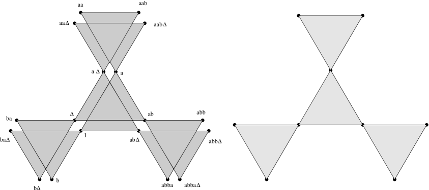
Figure 1: The graphs ${\mathcal{X}}(B_{3}/Z,S)$ (left) and ${\mathcal{S}}(C_{3},S)$ (right).

Let $\nu$ be a probability distribution on $S=\{a,a^{-1},b,b^{-1}\}$. Let $(X_{n})_{n}$ be a realization of $(B_{3},\nu)$. View $(X_{n})_{n}$ as a random walk on ${\mathcal{X}}(B_{3},S)$. The sequence $(p(X_{n}))_{n}$ is a realization of the random walk $(B_{3}/Z,\mu)$ where $\mu=\nu\circ p^{-1}$. It is a random walk on ${\mathcal{X}}(B_{3}/Z,S)$. Recall that $\widehat{X}_{n}\Delta^{k_{n}}$ denotes the Garside normal form of $X_{n}$. With the identification above, the random process $(\widehat{X}_{n})_{n}$ evolves on ${\mathcal{S}}(C_{3},S)$ and is the process induced by $(p(X_{n}))_{n}$. This random process $(\widehat{X}_{n})_{n}$ is a priori not Markovian, but it is Markovian if

$$\forall C,D\in C_{3},\forall c_{1},c_{2}\in C,\quad P\{p(X_{n+1})\in D\mid p(X_{n})=c_{1}\}=P\{p(X_{n+1})\in D\mid p(X_{n})=c_{2}\}\>.$$

Clearly, this holds if and only if $\nu(a)=\nu(b)=p$ and $\nu(a^{-1})=\nu(b^{-1})=1/2-p$, which is precisely what we assume.

Define ${\mathcal{S}}(C_{3},\mu)$ as the graph ${\mathcal{S}}(C_{3},S)$ with labels in $[0,1]$ such that:

$$u\stackrel{{\scriptstyle\mu(a)}}{{\longrightarrow}}v\ \text{ in }\ {\mathcal{S}}(C_{3},\mu)\qquad\text{if}\qquad u\stackrel{{\scriptstyle a}}{{\longrightarrow}}v\ \text{ in }\ {\mathcal{S}}(C_{3},S)\>.$$

Consider the group ${\mathbb{Z}}/3{\mathbb{Z}}\star{\mathbb{Z}}/3{\mathbb{Z}}$ with generators $\widetilde{S}=\{c,c^{-1},d,d^{-1}\}$, and the probability measure $\tilde{\mu}$ defined on $\widetilde{S}$ by $\tilde{\mu}(c)=\tilde{\mu}(d)=\nu(a)=\nu(b),$ and $\tilde{\mu}(c^{-1})=\tilde{\mu}(d^{-1})=\nu(a^{-1})=\nu(b^{-1})$. Define the labelled graph ${\mathcal{X}}({\mathbb{Z}}/3{\mathbb{Z}}\star{\mathbb{Z}}/3{\mathbb{Z}},\tilde{\mu})$ accordingly. Then ${\mathcal{S}}(C_{3},\mu)$ and ${\mathcal{X}}({\mathbb{Z}}/3{\mathbb{Z}}\star{\mathbb{Z}}/3{\mathbb{Z}},\tilde{\mu})$ are isomorphic as labelled graphs. In particular, $(\widehat{X}_{n})_{n}$ behaves like the random walk $({\mathbb{Z}}/3{\mathbb{Z}}\star{\mathbb{Z}}/3{\mathbb{Z}},\tilde{\mu})$. Let us be more precise.

For $\xi\in\widetilde{S}$, we set $\imath(\xi)=1$ if $\xi=c$ or $c^{-1}$ and $\imath(\xi)=2$ if $\xi=d$ or $d^{-1}$. Recall that $T=\{a,b,ab,ba\}\subset B_{3}$. Define

$$L=\{\xi_{0}\cdots\xi_{l}\in T^{*}\mid\text{Last}(\xi_{i})\>=\>\text{First}(\xi_{i+1})\}, L^{\infty}=\{\xi_{0}\cdots\in T^{{\mathbb{N}}}\mid\text{Last}(\xi_{i})\>=\>\text{First}(\xi_{i+1})\}$$

$$\widetilde{L}=\{\xi_{0}\xi_{1}\cdots\xi_{l}\in\widetilde{S}^{*}\mid\imath(\xi_{i})\>\neq\>\imath(\xi_{i+1})\}, \widetilde{L}^{\infty}=\{\xi_{0}\xi_{1}\cdots\in\widetilde{S}^{{\mathbb{N}}}\mid\imath(\xi_{i})\>\neq\>\imath(\xi_{i+1})\}\>.$$

Set $\lim_{n}\widehat{X}_{n}=\widehat{X}_{\infty}=\widehat{x}_{0}\widehat{x}_{1}\widehat{x}_{2}\cdots$, with $\widehat{x}_{i}\in T$. Let $\mu^{\infty}$ be the law of $\widehat{X}_{\infty}$; it is a measure on $L^{\infty}$. Let $\tilde{\mu}^{\infty}$ be the harmonic measure of $({\mathbb{Z}}/3{\mathbb{Z}}\star{\mathbb{Z}}/3{\mathbb{Z}},\tilde{\mu})$; it is a measure on $\widetilde{L}^{\infty}$. Let $\widetilde{r}$ be the unique solution in $\mathring{{\mathcal{B}}}$ of the Traffic Equations of $({\mathbb{Z}}/3{\mathbb{Z}}\star{\mathbb{Z}}/3{\mathbb{Z}},\tilde{\mu})$, see [7, §4.3]. Define

$$r(a)\>=\>r(b)\>=\>\tilde{r}(c)\>=\>\tilde{r}(d)\>,\>r(ab)\>=\>r(ba)\>=\>\tilde{r}(c^{2})\>=\>\tilde{r}(d^{2})\>,$$

$$r(1)\>=\>r(a)+r(b)\>,\>\text{and}\quad\>r(2)\>=\>r(ab)+r(ba)\>.$$

Then, we have, $\forall u_{1}\cdots u_{l}\in L$,

$$\mu^{\infty}(u_{1}u_{2}u_{3}\cdots u_{l}T^{{\mathbb{N}}})=\tilde{\mu}^{\infty}(c^{|u_{1}|_{S}}d^{|u_{2}|_{S}}c^{|u_{3}|_{S}}\cdots\widetilde{\Sigma}^{{\mathbb{N}}})=(1/2)r(|u_{1}|_{S})\cdots r(|u_{l}|_{S})\>.$$

In particular

$$\gamma_{\Sigma}=\lim_{n\rightarrow\infty}\frac{|\widehat{X}_{n}|_{T}}{n}=\lim_{n\rightarrow\infty}\frac{|W_{n}|_{\widetilde{S}}}{n}=pr(1)+\bigl{(}\frac{1}{2}-p\bigr{)}r(2)\>,$$ (4)

where $(W_{n})_{n}$ is a realization of the random walk $({\mathbb{Z}}/3{\mathbb{Z}}\star{\mathbb{Z}}/3{\mathbb{Z}},\tilde{\mu})$. See [7, Corollary 3.6] for the third equality in Eq. (4).

The vector $\tilde{r}$ is computed in [7, §4.3]:

$$\tilde{r}(c)=\tilde{r}(d)=\frac{4p-3+\sqrt{16p^{2}-8p+5}}{4(4p-1)},\quad\tilde{r}(c^{2})=\tilde{r}(d^{2})=\frac{4p+1-\sqrt{16p^{2}-8p+5}}{4(4p-1)}\>.$$ (5)

We get $\gamma_{\Sigma}\>=\>(-1+\sqrt{16p^{2}-8p+5})/4$. We deduce the other drifts easily.

4 Proof of Proposition 5.4

We now prove the following statement which is Prop. 5.4 in [8] :

Proposition 5.4 Consider the simple random walk $(A_{k},\nu)$ with $\nu(a)=\nu(a^{-1})=\nu(b)=\nu(b^{-1})=1/4$. The drifts $\gamma_{\Sigma}$ and $\gamma_{\Delta}$ are given by

$$\gamma_{\Sigma}=\frac{1-x_{k}}{2},\qquad\gamma_{\Delta}=-\frac{1-x_{k}}{4}\>.$$ (6)

Let $\gamma$ be the drift of the length with respect to the natural generators $\{a,b,a^{-1},b^{-1}\}$. We have

$$\gamma=\begin{cases}(1-x_{k})\bigl{[}\ \sum_{i=1}^{j-1}iF_{i}(x_{k})+(j/2)F_{j}(x_{k})\ \bigr{]}&\text{if }\ k=2j\\ (1-x_{k})\bigl{[}\ \sum_{i=1}^{j}iF_{i}(x_{k})\ \bigr{]}&\text{if }\ k=2j+1\end{cases}\>.$$ (7)

Proof.

Consider the group ${\mathbb{Z}}/k{\mathbb{Z}}\star{\mathbb{Z}}/k{\mathbb{Z}}$ with generators $\widetilde{S}=\{c,c^{-1},d,d^{-1}\}$. Let $(X_{n})_{n}$ be a realization of the simple random walk on $A_{k}$, and recall that we write $\widehat{X}_{n}\Delta^{k_{n}}$ for the Garside normal form of $X_{n}$. Denote by $\mu$ and $\tilde{\mu}$ the uniform probability measures on $S$ and $\widetilde{S}$ respectively.

If $k$ is even, then the unlabelled Cayley graph ${\mathcal{X}}(A_{k}/Z,S)$ is isomorphic to the unlabelled Cayley graph ${\mathcal{X}}({\mathbb{Z}}/k{\mathbb{Z}}\star Z/k{\mathbb{Z}},\widetilde{S})$ (see Figure 2) so the simple random walks $(A_{k}/Z,\mu)$ and $({\mathbb{Z}}/k{\mathbb{Z}}\star{\mathbb{Z}}/k{\mathbb{Z}},\tilde{\mu})$ are isomorphic.

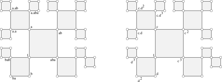
Figure 2: The Cayley graphs ${\mathcal{X}}(A_{4}/Z,S)$ (left) and ${\mathcal{X}}({\mathbb{Z}}/4{\mathbb{Z}}\star{\mathbb{Z}}/4{\mathbb{Z}},\widetilde{S})$ (right).

For $k$ odd, the structure of ${\mathcal{X}}(A_{k}/Z,S)$ is more twisted. This is illustrated in Figure 3 (see also Figure 1 (left)).

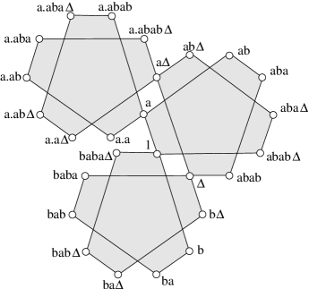
Figure 3: The Cayley graph ${\mathcal{X}}(A_{5}/Z,S)$.

Let $C_{k}$ be the left-quotient of $A_{k}/Z$ by the (non-normal) subgroup $H=\{1,\Delta\}$, and define the Schreier graph ${\mathcal{S}}(C_{k},S)$ as in (3). Clearly ${\mathcal{S}}(C_{k},S)$ is isomorphic to the Cayley graph ${\mathcal{X}}({\mathbb{Z}}/k{\mathbb{Z}}\star Z/k{\mathbb{Z}},\widetilde{S})$ (as unlabelled graphs). This is illustrated in Figure 4.

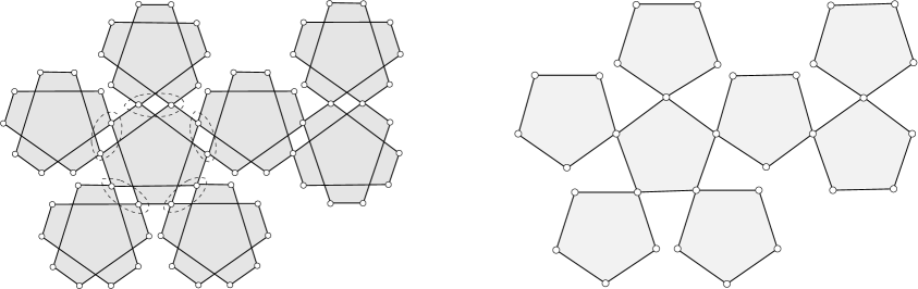
Figure 4: The graphs ${\mathcal{X}}(A_{5}/Z,S)$ (left) and ${\mathcal{S}}(C_{5},S)$ (right).

Therefore the simple random walks on the two graphs ${\mathcal{S}}(C_{k},S)$ and ${\mathcal{X}}({\mathbb{Z}}/k{\mathbb{Z}}\star Z/k{\mathbb{Z}},\widetilde{S})$ are isomorphic.

In both cases, the Markovian random process $\widehat{X}_{n}$ behaves like the simple random walk $({\mathbb{Z}}/k{\mathbb{Z}}\star{\mathbb{Z}}/k{\mathbb{Z}},\tilde{\mu})$. Adapting the end of the second proof of [8, Prop. 4.5] and using the results of [7, §4.4] leads to $\gamma_{\Sigma}$, hence to the other drifts. ∎

5 Extensions

One can retrieve from the harmonic measure $\mu^{\infty}$, other quantities of interest for the random walk $(B_{3}/Z,\mu)$: (a) the entropy, (b) the minimal positive harmonic functions, or (c) the Green function.

Consider for instance the entropy $h$. For NNRW on free products of finite groups, or on 0-automatic pairs, a formula was available for $h$ as a simple function of $r$, the unique solution to the Traffic Equations, see [6, 7]. Here the situation is more complex and $h$ can only be expressed as a limit of functions of $r$. However $h$ can be computed with an arbitrary prescribed precision.

In the three above cases (a), (b), and (c), the key is to determine the Radon-Nikodym derivatives $du\circledast\mu^{\infty}/d\mu^{\infty}(\cdot)$ for $u\in{\mathcal{G}}$.

Fix $u=u_{1}\cdots u_{k}\in{\mathcal{G}}$ and $\xi=\xi_{1}\xi_{2}\cdots\in{\mathcal{G}}^{\infty}$. We have, using [8, (21)],

$$\frac{du\circledast\mu^{\infty}}{d\mu^{\infty}}(\xi)=\lim_{n}\frac{\mu^{\infty}(u^{-1}\circledast\xi_{1}\cdots\xi_{n}T^{{\mathbb{N}}})}{\mu^{\infty}(\xi_{1}\cdots\xi_{n}T^{{\mathbb{N}}})}=\lim_{n}\frac{\alpha{\mathcal{M}}(w_{1}\cdots w_{\ell-1})\beta(w_{\ell})}{\alpha{\mathcal{M}}(\xi_{1}\cdots\xi_{n-1})\beta(\xi_{n})}\>,$$ (8)

where $w_{1}\cdots w_{\ell}=u^{-1}\circledast\xi_{1}\cdots\xi_{n}$. Below, we justify the existence of the limit in (8), and in doing so we show how to control the error made when replacing the limit by the value computed for a given $n$.

It follows from the definition in [8, (9)] that we have either:

$$u^{-1}\circledast\xi_{1}\cdots\xi_{n}=v\cdot\xi_{l}\cdot\ldots\cdot\xi_{n},\quad\text{or}\quad u^{-1}\circledast\xi_{1}\cdots\xi_{n}=v\cdot\iota(\xi_{l})\cdot\ldots\cdot\iota(\xi_{n})\>,$$

for some $v\in{\mathcal{G}}$ and $l\in{\mathbb{N}}^{*}$ which do not depend on $n$, for $n$ large enough. In the first case, respectively the second one, we have:

$$\frac{du\circledast\mu^{\infty}}{d\mu^{\infty}}(\xi) = \lim_{n}\ \frac{\alpha{\mathcal{M}}(v\xi_{\ell}\cdots\xi_{n-1})\beta(\xi_{n})}{\alpha{\mathcal{M}}(\xi_{1}\cdots\xi_{n-1})\beta(\xi_{n})}$$ (9)

$$\text{resp. }\ \frac{du\circledast\mu^{\infty}}{d\mu^{\infty}}(\xi) = \lim_{n}\ \frac{\alpha{\mathcal{M}}(v\iota(\xi_{\ell})\cdots\iota(\xi_{n-1}))\beta(\iota(\xi_{n}))}{\alpha{\mathcal{M}}(\xi_{1}\cdots\xi_{n-1})\beta(\xi_{n})}\>.$$ (10)

Now, the ${\mathbb{R}}_{+}$-automaton $(\alpha,{\mathcal{M}},\beta)$ of [8, Figure 9] has several remarkable properties. Define $\iota(\alpha)=[0,1,0,1]\in{\mathbb{R}}_{+}^{1\times Q}$. Observe that $\iota(\alpha)_{i}=\alpha_{5-i}$. Observe also that: $\forall u\in\Sigma,\forall i,j,\ {\mathcal{M}}(u)_{ij}={\mathcal{M}}(\iota(u))_{5-i,5-j}$. It implies that we have:

$$\forall u=u_{1}\cdots u_{k}\in T^{*},\qquad\alpha{\mathcal{M}}(u_{1}\cdots u_{k-1})\beta(u_{k})=\iota(\alpha){\mathcal{M}}(\iota(u_{1})\cdots\iota(u_{k-1}))\beta(\iota(u_{k}))\>.$$ (11)

Extend by morphism the map $\iota$ defined in [8, (10)] to $\iota:\Sigma^{*}\longrightarrow\Sigma^{*}$. The identity in (11) enables to rewrite (10) as:

$$\frac{du\circledast\mu^{\infty}}{d\mu^{\infty}}(\xi)=\lim_{n}\ \frac{\iota(\alpha){\mathcal{M}}(\iota(v)\xi_{\ell}\cdots\xi_{n-1})\beta(\xi_{n})}{\alpha{\mathcal{M}}(\xi_{1}\cdots\xi_{n-1})\beta(\xi_{n})}\>.$$

To summarize, in all cases, for $n$ large enough, there exist $l\in{\mathbb{N}}^{*}$ and $\alpha_{1}\in{\mathbb{R}}_{+}^{1\times Q}$ such that:

$$\frac{du\circledast\mu^{\infty}}{d\mu^{\infty}}(\xi)=\lim_{n}\ \frac{\alpha_{1}{\mathcal{M}}(\xi_{\ell}\cdots\xi_{n-1})\beta(\xi_{n})}{\alpha_{2}{\mathcal{M}}(\xi_{\ell}\cdots\xi_{n-1})\beta(\xi_{n})}\>,$$ (12)

with $\alpha_{2}=\alpha{\mathcal{M}}(\xi_{1}\cdots\xi_{\ell-1})$. The limit in (12) exists as a consequence of general results on inhomogeneous products of non-negative matrices, see for instance [10, Chapter 3]. To be more precise, and to evaluate the speed of convergence, it is convenient to slightly rewrite (12), in order to have matrices with positive entries.

Consider the automaton $(\widetilde{\alpha},\widetilde{{\mathcal{M}}},\widetilde{\beta})$ defined as follows. Set $\widetilde{\alpha}=[1,1]$; for $u\in T$, set $\widetilde{\beta}(u)=[R(u),R(u)]^{T}$; and let the morphism $\widetilde{{\mathcal{M}}}:T^{*}\rightarrow{\mathbb{R}}_{+}^{2\times 2}$ be defined by:

$$\widetilde{{\mathcal{M}}}(a)=\left[\begin{array}[]{cc}q(a)&q(a\Delta)\\ q(b\Delta)&q(b)\end{array}\right]\>,\quad\widetilde{{\mathcal{M}}}(b)=\ \left[\begin{array}[]{cc}q(b)&q(b\Delta)\\ q(a\Delta)&q(a)\end{array}\right]$$

$$\widetilde{{\mathcal{M}}}(ab)=\ \left[\begin{array}[]{cc}q(ab)&q(ab\Delta)\\ q(ba\Delta)&q(ba)\end{array}\right]\>,\quad\widetilde{{\mathcal{M}}}(ba)=\ \left[\begin{array}[]{cc}q(ba)&q(ba\Delta)\\ q(ab\Delta)&q(ab)\end{array}\right]\>.$$

It is easily checked that, on ${\mathcal{G}}$, the two automata $(\widetilde{\alpha},\widetilde{{\mathcal{M}}},\widetilde{\beta})$ and $(\alpha,{\mathcal{M}},\beta)$ coincide. That is:

$$\forall u=u_{1}\cdots u_{k}\in{\mathcal{G}},\quad\widetilde{\alpha}\widetilde{{\mathcal{M}}}(u_{1}\cdots u_{k-1})\widetilde{\beta}(u_{k})=\alpha{\mathcal{M}}(u_{1}\cdots u_{k-1})\beta(u_{k})\>.$$ (13)

Observe that the above identity does not hold on $T^{*}{\setminus}{\mathcal{G}}$. (In fact, the automaton $(\alpha,{\mathcal{M}},\beta)$ is the tensor product of $(\widetilde{\alpha},\widetilde{{\mathcal{M}}},\widetilde{\beta})$ with a 2-state automaton recognizing ${\mathcal{G}}\cap T^{*}$.)

Define:

$$\delta=\min_{u\in\Sigma}\frac{\min_{ij}\widetilde{{\mathcal{M}}}(u)_{ij}}{\max_{ij}\widetilde{{\mathcal{M}}}(u)_{ij}},\quad K=\max_{u\in\Sigma}\max_{ij}\Bigl{[}\max_{k}\frac{\widetilde{{\mathcal{M}}}(u)_{ik}}{\widetilde{{\mathcal{M}}}(u)_{jk}}-\min_{k}\frac{\widetilde{{\mathcal{M}}}(u)_{ik}}{\widetilde{{\mathcal{M}}}(u)_{jk}}\Bigr{]}\>.$$

Observe that $0<\delta<1$. For $x=x_{1}x_{2}\cdots\in T^{{\mathbb{N}}}$, set

$$c(x)=\bigl{[}1,\lim_{n}\widetilde{{\mathcal{M}}}(x_{1}\cdots x_{n})_{2k}/\widetilde{{\mathcal{M}}}(x_{1}\cdots x_{n})_{1k}\bigl{]}^{T}\>,$$

where the limit does not depend on $k\in\{1,2\}$. Using [10, Exercice 3.9], we get, for $k\in\{1,2\}$,

$$\Bigl{|}\ \frac{\widetilde{{\mathcal{M}}}(x_{1}\cdots x_{n})_{2k}}{\widetilde{{\mathcal{M}}}(x_{1}\cdots x_{n})_{1k}}-c(x)_{2}\ \Bigr{|}\leq K(1-\delta^{2})^{n-1}\>.$$ (14)

Now let us go back to (12). Set $\eta=\eta_{1}\eta_{2}\cdots=\xi_{\ell}\xi_{\ell+1}\cdots$. For $x=(x_{1},x_{2})\in{\mathbb{R}}^{2},$ set $\|x\|=|x_{1}|+|x_{2}|$; for $x=(x_{1},x_{2}),y=(y_{1},y_{2})\in{\mathbb{R}}^{2},$ set $\langle x,y\rangle=x_{1}y_{1}+x_{2}y_{2}$. We have:

$$\frac{du\circledast\mu^{\infty}}{d\mu^{\infty}}(\xi)=\lim_{n}\frac{\widetilde{\alpha}_{1}\widetilde{{\mathcal{M}}}(\xi_{\ell}\cdots\xi_{n})\widetilde{\beta}(\xi_{n+1})}{\widetilde{\alpha}_{2}\widetilde{{\mathcal{M}}}(\xi_{\ell}\cdots\xi_{n})\widetilde{\beta}(\xi_{n+1})}=\frac{\langle\widetilde{\alpha}_{1},c(\eta)\rangle}{\langle\widetilde{\alpha}_{2},c(\eta)\rangle}\>.$$

Let us fix $n$ larger than $\ell$. Set $\varepsilon=K(1-\delta^{2})^{n-\ell-1}$. Using (14), we easily get:

$$\frac{\langle\widetilde{\alpha}_{1},c(\eta)\rangle-\varepsilon\|\widetilde{\alpha}_{1}\|}{\langle\widetilde{\alpha}_{2},c(\eta)\rangle+\varepsilon\|\widetilde{\alpha}_{2}\|}\ \leq\ \frac{\widetilde{\alpha}_{1}\widetilde{{\mathcal{M}}}(\xi_{\ell}\cdots\xi_{n})\widetilde{\beta}(\xi_{n+1})}{\widetilde{\alpha}_{2}\widetilde{{\mathcal{M}}}(\xi_{\ell}\cdots\xi_{n})\widetilde{\beta}(\xi_{n+1})}\ \leq\ \frac{\langle\widetilde{\alpha}_{1},c(\eta)\rangle+\varepsilon\|\widetilde{\alpha}_{1}\|}{\langle\widetilde{\alpha}_{2},c(\eta)\rangle-\varepsilon\|\widetilde{\alpha}_{2}\|}\>.$$

The above inequalities provide a sharp control on the error made when replacing the limit in (12) by the value computed for a fixed $n$.

Entropy

The entropy of a probability measure $\mu$ with finite support $S$ is defined by $H(\mu)=-\sum_{x\in S}\mu(x)\log[\mu(x)]$. Consider a random walk $(G,\mu)$, defined as in [8, Section 2]. Let $(X_{n})_{n}$ be a realization of the random walk. The entropy of $(G,\mu)$, introduced by Avez [1], is

$$h=\lim_{n}\frac{H(\mu^{*n})}{n}=\lim_{n}-\frac{1}{n}\log\mu^{*n}(X_{n})\>,$$ (15)

$a.s.$ and in $L^{p}$, for all $1\leq p<\infty$. The existence of the limits as well as their equality follow from Kingman’s subadditive ergodic theorem [1, 2].

Consider the random walk $(B_{3}/Z,\mu)$. Recall that $({\mathcal{G}}^{\infty},\mu^{\infty})$ is the Poisson boundary of $(B_{3}/Z,\mu)$. Then, we have, see [4, Theorem 3.1]:

$$h=-\sum_{u\in\Sigma}\mu(u)\int\log\bigl{[}\frac{du^{-1}\circledast\mu^{\infty}}{d\mu^{\infty}}(\xi)\bigr{]}d\mu^{\infty}(\xi)\>.$$ (16)

Using (16) together with the above remarks on how to approximate the Radon-Nikodym derivatives, one can derive an algorithm to compute $h$ with an arbitrarily prescribed precision.

Minimal positive harmonic functions

Consider a random walk $(G,\mu)$ defined as in [8, Section 2]. A positive harmonic function is a function $f:G\rightarrow{\mathbb{R}}_{+}$ such that: $\forall u\in G,\ \sum_{a\in\Sigma}f(u\ast a)\mu(a)=f(u)$. A positive harmonic function $f$ is minimal if $f(1)=1$ and if for any positive harmonic function $g$ such that $f\geq g$, there exists $c\in{\mathbb{R}}_{+}$ such that $f=cg$.

Consider the random walk $(B_{3}/Z,\mu)$ as above. Recall that ${\mathcal{G}}^{\infty}$ is the minimal Martin boundary of $(B_{3}/Z,\mu)$. So the set of minimal positive harmonic function is precisely given by $\{K_{\xi},\xi\in{\mathcal{G}}^{\infty}\}$ with

$$K_{\xi}:B_{3}/Z\rightarrow{\mathbb{R}}_{+},\quad K_{\xi}(g)=\frac{d\phi(g)\circledast\mu^{\infty}}{d\mu^{\infty}}(\xi)\>.$$ (17)

Green function

Consider a transient random walk $(G,\mu)$ defined as in [8, Section 2] and a realization $(X_{n})_{n}$. Define, $Q:G\rightarrow[0,1],$

$$Q(g)=P\{\exists n\geq 1\mid X_{n}=g\}\>,$$ (18)

the probability of ever reaching $g$. The Green function is the map $\Gamma:G\rightarrow{\mathbb{R}}_{+},\ \Gamma(g)=\sum_{i=0}^{\infty}\mu^{*i}(g)$. Observe that:

$$\Gamma(\cdot)=\Gamma(1)Q(\cdot)\>.$$ (19)

Consider now the random walk $(B_{3}/Z,\mu)$. Computing $Q$ is more involved than for free groups [3] or for zero-automatic pairs [6]. However, the spirit remains the same: there is a close link between $Q$ and $r$, the unique solution to the Traffic Equations.

For convenience, we view $Q$ and $\Gamma$ as $Q:{\mathcal{G}}\rightarrow{\mathbb{R}}_{+}$ and $\Gamma:{\mathcal{G}}\rightarrow{\mathbb{R}}_{+}$. Define, for $u\in{\mathcal{G}}$, the auxiliary quantity:

$$\widehat{q}(u) = P\{\exists n>1\mid Y_{n}=u\ \text{ and }\ \forall 1<m<n,Y_{m}\neq u\Delta\}\>.$$ (20)

We have the following:

Proposition 5.1.

Let $r\in\{x\in({\mathbb{R}}_{+}^{*})^{\Sigma}\mid\sum_{u\in\Sigma}x(u)=1\}$ be the unique solution to the Traffic Equations [8, (19)] of $(B_{3}/Z,\mu)$. For $u\in\Sigma$, set $q(u)=r(u)/r(\text{Next}(u))$. We have:

$$\forall u\in\Sigma,\quad\widehat{q}(u)=\frac{r(u)}{r(\text{Next}(u))}=q(u)\>.$$ (21)

Besides:

$$\widehat{q}(1)=\sum_{u\in\Sigma}\mu(u)q(u^{-1}),\quad\widehat{q}(\Delta)=\sum_{u\in\Sigma}\mu(u)q(u^{-1}\Delta)\>.$$ (22)

The probabilities of ever reaching an element are given by: $Q(\Delta)=\widehat{q}(\Delta)/(1-\widehat{q}(1))$, and, $\forall v=v_{1}\cdots v_{k}\in{\mathcal{G}}{\setminus}\{1,\Delta\}$:

$$Q(v)=\sum_{u_{1}\cdots u_{k}\in\psi^{-1}(v)}q(u_{1})\cdots q(u_{k-1})\bigl{[}q(u_{k})+q(u_{k}\Delta)Q(\Delta)\bigr{]}\>.$$ (23)

The Green function is determined by (19) and:

$$\Gamma(1)=\frac{1-\widehat{q}(1)}{(1-\widehat{q}(1))^{2}-\widehat{q}(\Delta)^{2}}\>.$$ (24)

(See [8, Eq. (13)] for the definition of $\psi$)

Proof.

It follows from the shape of the Cayley graph ${\mathcal{X}}(B_{3}/Z,\Sigma)$ that:

$$\widehat{q}(1)=\sum_{u\in\Sigma}\mu(u)\widehat{q}(u^{-1}),\quad\widehat{q}(\Delta)=\sum_{u\in\Sigma}\mu(u)\widehat{q}(u^{-1}\Delta),\quad Q(\Delta)=\widehat{q}(\Delta)/(1-\widehat{q}(1))\>.$$

Similarly, (23) holds with $\widehat{q}(\cdot)$ in place of $q(\cdot)$. Let us prove (24). Define $\bar{Q}(1)=P\{\exists n>1\mid Y_{n}=1\}$. Clearly, $\bar{Q}(1)=\widehat{q}(1)+\widehat{q}(\Delta)Q(\Delta)$ and $\Gamma(1)=1+\bar{Q}(1)\Gamma(1)$. The expression in (24) follows. Therefore, the only point that remains to be proved is: $\forall u\in\Sigma,\widehat{q}(u)=q(u)$.

For $u\in\Sigma$, define $F_{u}=\{v\in\Sigma\mid\text{First}(v)=\text{First}(u)\}$. By considering the random walk after one move, we get that $(\widehat{q}(u))_{u\in\Sigma}$ is a solution to the following equations over the indeterminates $(y(u))_{u\in\Sigma}$:

$$y(u)=\mu(u)+\sum_{v\in F_{u}{\setminus}\{u,u\Delta\}}\mu(v)y(v^{-1}u)+\sum_{v\in\Sigma{\setminus}F_{u}}\mu(v)\bigl{[}y(v^{-1})y(u)+y(v^{-1}\Delta)y(\iota(u)\Delta)\bigr{]}\>.$$ (25)

Starting from the Traffic Equations [8, (19)], and dividing by $x(\text{Next}(u))$, we obtain precisely the Equations (25). Let $r\in\{x\in({\mathbb{R}}_{+}^{*})^{\Sigma}\mid\sum_{u\in\Sigma}x(u)=1\}$ be the unique solution to the Traffic Equations, and set $q(u)=r(u)/r(\text{Next}(u))$ for $u\in\Sigma$. We deduce from the above that $(q(u))_{u\in\Sigma}$ is a solution to the Equations (25).

We cannot directly conclude that $\widehat{q}(u)=q(u)$. Indeed the Equations (25) do not characterize $(\widehat{q}(u))_{u\in\Sigma}$. They have in general several solutions in $(0,1)^{\Sigma}$ (if $\mu$ is uniform over $\Sigma$, then the two constant functions $y=1/2$ and $y=1/4$ satisfy (25)). This is in contrast with the situation for 0-automatic pairs where the analogs of Equations (25) have a unique solution [6, Lemma 4.7].

Recall that the minimal Martin boundary coincides with the Martin boundary and is ${\mathcal{G}}^{\infty}$. Hence, the minimal positive harmonic functions, given in (17), can also be described as: $\forall\xi=\xi_{1}\cdots\in{\mathcal{G}}^{\infty}$,

$$K_{\xi}:B_{3}/Z\rightarrow{\mathbb{R}}_{+},\quad K_{\xi}(g)=\lim_{n}\frac{\Gamma(\phi(g^{-1})\circledast\xi_{1}\cdots\xi_{n})}{\Gamma(\xi_{1}\cdots\xi_{n})}=\lim_{n}\frac{Q(\phi(g^{-1})\circledast\xi_{1}\cdots\xi_{n})}{Q(\xi_{1}\cdots\xi_{n})}\>.$$ (26)

Juxtaposing (17) and (26), and using [8, (20)] and (23) (with $\widehat{q}(\cdot)$ replacing $q(\cdot)$), we get: for all $u\in B_{3}/Z$ and $\xi=\xi_{1}\xi_{2}\cdots\in{\mathcal{G}}^{\infty}$,

$$K_{\xi}(u) = \lim_{n}\ \frac{\sum_{v_{1}\cdots v_{\ell}\in\psi^{-1}(\phi(u^{-1})\circledast\xi_{1}\cdots\xi_{n})}q(v_{1})\cdots q(v_{\ell-1})R(v_{\ell})}{\sum_{v_{1}\cdots v_{n}\in\psi^{-1}(\xi_{1}\cdots\xi_{n})}q(v_{1})\cdots q(v_{n-1})R(v_{n})}$$

$$= \lim_{n}\ \frac{\sum_{v_{1}\cdots v_{\ell}\in\psi^{-1}(\phi(u^{-1})\circledast\xi_{1}\cdots\xi_{n})}\widehat{q}(v_{1})\cdots\widehat{q}(v_{\ell-1})Q(v_{\ell})}{\sum_{v_{1}\cdots v_{n}\in\psi^{-1}(\xi_{1}\cdots\xi_{n})}\widehat{q}(v_{1})\cdots\widehat{q}(v_{n-1})Q(v_{n})}\>.$$

By choosing appropriately the values of $u$, we deduce easily that this implies $q(\cdot)=\widehat{q}(\cdot)$. ∎

Central Limit Theorem

Recall that we write $\widehat{X}_{n}\Delta^{k_{n}}$ for the Garside normal form of $X_{n}$. The description of the asymptotic behavior the quotient process $(p(X_{n}))$ evolving on $B_{3}/Z$ provides a Central Limit Theorem for both the length $|\widehat{X}_{n}|_{T}$ and the exponent $k_{n}$ in the same way as in [5].

The statement is the following. Recall that we set $U=p^{-1}(\Sigma)=\{a\Delta^{k},ab\Delta^{k},b\Delta^{k},$ $ba\Delta^{k},k\in{\mathbb{Z}}\}$ and $T=\{a,b,ab,ba\}\subset B_{3}$

Proposition 5.2.

Consider the random walk $(B_{3},\nu)$ where $\nu$ is a probability measure on $U$ such that $\cup_{n}\text{supp}(\nu^{*n})=B_{3}$ and $\sum_{x\in U}e^{\lambda|x|_{S}}\nu(x)<\infty$ for some $\lambda>0$. Let $(X_{n})$ be a realization of the random walk $(B_{3},\nu)$ and $\widehat{X}_{n}\Delta^{k_{n}}$ the Garside normal form of $X_{n}$. Then there exist two positive numbers $\sigma_{\Sigma}$ and $\sigma_{\Delta}$ such that, for all $t\in{\mathbb{R}}$,

$$\lim_{n\to+\infty}{P\biggl{\{}\frac{|\widehat{X}_{n}|_{T}-n\gamma_{\Sigma}}{\sigma_{\Sigma}\sqrt{n}}<t\biggr{\}}}\>=\>\lim_{n\to+\infty}{P\biggl{\{}\frac{k_{n}-n\gamma_{\Delta}}{\sigma_{\Delta}\sqrt{n}}<t\biggr{\}}}\>=\>\frac{1}{\sqrt{2\pi}}\int_{-\infty}^{t}e^{-x^{2}/2}\text{d}x\>\>.$$ (27)

As far as $k_{n}$ is concerned, starting from the proof of [8, Lemma 4.10], one can easily adapt the techniques developped in [5, Section 4.c] to prove the result. The proof of the statement for $|\widehat{X}_{n}|_{T}$ is analogous, the function $\theta_{\Delta}$ has to be replaced by a function $\theta_{\Sigma}\>:\>U^{{\mathbb{N}}}\times{\mathcal{G}}^{\infty}\rightarrow{\mathbb{Z}}$ defined, for all $(\omega,\xi)\in U^{{\mathbb{N}}}\times{\mathcal{G}}^{\infty}$, by

$$\theta_{\Sigma}(\omega,\xi)=\begin{cases}+1&\mbox{if}\>\>\omega_{0}\ast\xi_{0}\not\in\Sigma\cup\{1,\Delta\}\\ -1&\mbox{if}\>\>\omega_{0}\ast\xi_{0}\>=\>1\>\mbox{or}\>\Delta\\ 0&\mbox{if}\>\>\omega_{0}\ast\xi_{0}\in\Sigma\end{cases}\>,\>\>\mbox{where}\>\omega\>=\>(\omega_{0},\omega_{1},...)\>.$$

That is, $\theta_{\Sigma}(\omega,\xi)$ counts the variation of the length of $\xi$ when it is left-multiplied by $\omega_{0}$. Integrating $\theta_{\Sigma}$ over $U^{{\mathbb{N}}}\times{\mathcal{G}}^{\infty}$ leads to the drift $\gamma_{\Sigma}$, exactly as in [8, Lemma 4.10].

References

[1]
A. Avez.
Entropie des groupes de type fini.
C. R. Acad. Sci. Paris Sér. A-B, 275:1363–1366,
1972.
[2]
Y. Derriennic.
Quelques applications du théorème ergodique sous-additif.
Astérisque, 74:183–201, 1980.
[3]
E. Dynkin and M. Malyutov.
Random walk on groups with a finite number of generators.
Sov. Math. Dokl., 2:399–402, 1961.
[4]
V. Kaimanovich and A. Vershik.
Random walks on discrete groups: boundary and entropy.
Ann. Probab., 11(3):457–490, 1983.
[5]
F. Ledrappier.
Some asymptotic properties of random walks on free groups.
In J. Taylor, editor, Topics in probability and Lie groups:
boundary theory, number 28 in CRM Proc. Lect. Notes, pages 117–152.
American Mathematical Society, 2001.
[6]
J. Mairesse.
Random walks on groups and monoids with a Markovian harmonic
measure.
Electron. J. Probab., 10:1417–1441, 2005.
[7]
J. Mairesse and F. Mathéus.
Random walks on free products of cyclic groups.
arXiv:math.PR/0509211, 2005.
To appear in J. London Math. Soc., 2007.
Appendix to the paper : arXiv:math.PR/0509208, 2005.
[8]
J. Mairesse and F. Mathéus.
Randomly growing braid on three strands and the manta ray.
To appear in Ann. Appl. Prob., 2007.
[9]
J. Mairesse and F. Mathéus.
Growth series for Artin groups of dihedral type.
Internat. J. Algebra
Comput., 16(6):1087-1107, 2006.
[10]
E. Seneta.
Non-negative Matrices and Markov Chains.
Springer Series in Statistics. Springer-Verlag, Berlin, 1981.