A quantitative investigation into the accumulation of rounding errors in the numerical solution of ODEs

Abstract

We examine numerical rounding errors of some deterministic solvers for systems of ordinary differential equations (ODEs). We show that the accumulation of rounding errors results in a solution that is inherently random and we obtain the theoretical distribution of the trajectory as a function of time, the step size and the numerical precision of the computer. We consider, in particular, systems which amplify the effect of the rounding errors so that over long time periods the solutions exhibit divergent behaviour. By performing multiple repetitions with different values of the time step size, we observe numerically the random distributions predicted theoretically. We mainly focus on the explicit Euler and RK4 methods but also briefly consider more complex algorithms such as the implicit solvers VODE and RADAU5.

Abbreviated Title: Rounding errors in the numerical solution of ODEs

1 Introduction

Consider ordinary differential equations (ODEs) of the form

$$\dot{x}_{t}=b(x_{t}).$$

These can be solved numerically using iteration methods of the type

$$x_{t+h}=x_{t}+\beta(h,x_{t})$$

where $\beta(h,x)/h\to b(x)$ as $h\to 0$.

The simplest example of this is the Euler method where $\beta(h,x)=hb(x)$. This method is generally not used in practice as it is relatively inaccurate and unstable compared to other methods. However more practical methods, such as the fourth order Runge-Kutta formula (RK4), fall into this scheme.

When solving an ordinary differential equation numerically, each time an iteration is performed, an error $\epsilon$ is incurred due to rounding i.e.

$$X^{h}_{t+h}=X^{h}_{t}+\beta(h,X^{h}_{t})+\epsilon.$$ (1)

Rounding errors in numerical computations are an inevitable consequence of finite precision arithmetic. The first work thoroughly analysing the effects of rounding errors on numerical algorithms is the classical textbook [16]. A recent comprehensive treatment of the behaviour of numerical algorithms in finite precision including an extensive list of references can be found in [11]. Although rounding errors are not random in the sense that the exact error incurred in any given calculation is fully determined (see [11] or [4]), probabilistic models have been shown to adequately describe their behaviour. In fact, statistical analysis of rounding errors can be traced back to one of the first works on rounding error analysis [5].

Henrici [7; 8; 9] proposes a probabilistic model for the individual rounding errors, whereby they are independent and uniform, the exact distribution depending on the specific finite precision arithmetic being used. Using the central limit theorem he shows that the theoretical distribution of the error accumulated after a fixed number of steps in the numerical solution of an ODE is asymptotically normal with variance proportional to $h^{-1}$. By varying the initial conditions he obtains numerical distributions for the accumulated errors, with good agreement. Hull and Swenson [12] test the validity of the above model by adding a randomly generated error with the same distribution at each stage of the calculation, and comparing the distribution of the accumulated errors with those obtained purely by rounding. They observe that although rounding is neither a random process nor are successive errors independent, probabilistic models appear to provide a good description of what actually happens.

We shall concentrate on floating point arithmetic, as used by modern computers. However, our methods can be used equally well for any finite precision arithmetic. We use the model, discussed and tested by the authors above, whereby under generic conditions, the errors in (1) can be viewed as independent, zero mean, uniform random variables $\epsilon_{i}\sim U[-|X^{h}_{t,i}|2^{-p},|X^{h}_{t,i}|2^{-p}]$, $p$ being a constant determined by the precision of the computer.

In the first half of the paper we analyse the cumulative effect of these rounding errors as the step size $h\to 0$. Where previous authors have considered the accumulated error at a particular point, we derive a theoretical model for the entire trajectory. Cases in $\mathbb{R}^{2}$ where the ordinary differential equation has a saddle fixed point at the origin exhibit the most interesting behaviour, as the structure of the ODE system amplifies the effect of the rounding errors and causes the numerical solution to diverge from the actual solution. We show that in this case the solution $X^{h}_{t}$ is inherently random and we obtain its theoretical distribution as an explicit function of time, the step size and the precision of the computer. We shall see that as the step size $h\to 0$, the numerical solution exhibits three types of behaviour, depending on the time. More precisely, there exists a constant $c$, determined by the ODE system, such that for times much smaller than $-c\log h$ the numerical solution converges to the actual solution; for times close to $-c\log h$ the solution undergoes a transition, driven by a Gaussian random variable whose distribution we shall obtain; for times much larger than $-c\log h$ the numerical solution diverges from the actual solution.

In the second half of the paper, we perform numerical simulations which illustrate this behaviour. By performing multiple repetitions with different values of the time step size, we observe the random distributions predicted theoretically. Where previous authors have obtained their numerical distributions by varying the initial conditions, we do so by introducing small variations in the step size $h$. We show that during the transition period described in the previous paragraph, the numerical solution intersects straight lines through the origin and we compare the theoretical and numerical distributions for the points at which these intersections occur. Both the mean and the standard deviation of these distributions are of the form $ah^{\gamma}$, where $\gamma\in(0,1/2]$ is a constant determined by the ODE system, and $a$ can be found explicitly in terms of the precision of the computer, i.e. the number of bits used internally by the computer to represent floating point numbers. We mainly focus on the explicit Euler and RK4 methods, but show that the same behaviour is also observable for more complex algorithms such as the implicit solvers VODE and RADAU5.

2 Theoretical background

In the paper [15], limiting results are established for sequences of Markov processes that approximate solutions of ordinary differential equations with saddle fixed points. We shall outline these results and then show that the rounding errors accumulated when performing numerical schemes for solving ordinary differential equations can be viewed as a special case of this. This enables us to quantify how the rounding errors combine, and show that the resulting numerical solutions exhibit random behaviour, the exact distribution of which is obtained.

2.1 Behaviour of stochastic jump processes

We are interested in ordinary differential equations of the form

$$\dot{x}_{t}=b(x_{t}).$$ (2)

We focus on $\mathbb{R}^{2}$ in the case where the origin is a saddle fixed point of the system i.e. $b(x_{t})=Bx_{t}+\tau(x_{t})$, where $B$ is a matrix with eigenvalues $\lambda,-\mu$, with $\lambda,\mu>0$ and $\tau(x)=O(|x|^{2})$ is twice continuously differentiable. This case is of particular interest as the structure of the system amplifies the effect of the rounding errors and causes the numerical solution to diverge from the actual solution over large times. Similar behaviour can be observed in higher dimensions where the matrix $B$ has at least one positive and one negative eigenvalue, although the corresponding quantitative analysis is much harder and we do not go into it here.

The phase portrait of (2) in the neighbourhood of the origin is shown in Figure 1.

Figure 1: The phase portrait of an ordinary differential equation having a saddle fixed point at the origin (taken from [15]).

In particular, there exists some $x_{0}\neq 0$ such that $\phi_{t}(x_{0})\rightarrow 0$ as $t\rightarrow\infty$, where $\phi$ is the flow associated with the ordinary differential equation (2). The set of such $x_{0}$ is the stable manifold. There also exists some $x_{\infty}$ such that $\phi^{-1}_{t}(x_{\infty})\rightarrow 0$ as $t\rightarrow\infty$. The set of such $x_{\infty}$ is the unstable manifold.

Fix an $x_{0}$ in the stable manifold and consider sequences $X_{t}^{N}$ of Markov processes starting from $x_{0}$, which converge to the solution of (2) over compact time intervals. The processes are indexed so that the variance of the fluctuations of $X_{t}^{N}$ is inversely proportional to $N$. If we allow the value of $t$ to grow with $N$ as a constant times $\log N$, $X_{t}^{N}$ deviates from the stable solution to a limit which is inherently random, before converging to an unstable solution (see Figure 2).

Figure 2: Diagram showing how the Markov process $X_{t}^{N}$ deviates from the stable solution $\phi_{t}(x_{0})$ for large values of $t$ (taken from [15]).

More precisely, we observe three different types of behaviour depending on the time scale:

1. On compact time intervals, $X_{t}^{N}$ converges to the stable solution of (2), the fluctuations around this limit being of order $N^{-\frac{1}{2}}$. The exact distribution of the fluctuations is asymptotically $N^{-\frac{1}{2}}\gamma_{t}$ where $\gamma_{t}$ is the solution to a linear stochastic differential equation, described in [15].

2. Let $v_{1}$ and $v_{2}$ be the unit eigenvectors of $B$ corresponding to $-\mu$ and $\lambda$ respectively. There exists some $\overline{x}_{0}\neq 0$, depending only on $x_{0}$, and a Gaussian random variable $Z_{\infty}$, such that if $t$ lies in the interval $[R,\frac{1}{2\lambda}\log N-R]$, then

   $$X_{t}^{N}=\overline{x}_{0}e^{-\mu t}(v_{1}+\epsilon_{1})+N^{-\frac{1}{2}}Z_{\infty}e^{\lambda t}(v_{2}+\epsilon_{2})$$

   where $\epsilon_{i}(t,N)\rightarrow 0$ uniformly in $t$ in probability as $R,N\rightarrow\infty$. In other words, $X_{t}^{N}$ can be approximated by the solution to the linear ordinary differential equation

   $$\dot{y_{t}}=By_{t}$$ (3)

   starting from the random point $\overline{x}_{0}v_{1}+N^{-\frac{1}{2}}Z_{\infty}v_{2}$.

3. Provided $Z_{\infty}\neq 0$, on time intervals of a fixed length around $\frac{1}{2\lambda}\log N$, $X_{t}^{N}$ converges to one of the two unstable solutions of (2), each with probability $1/2$, depending on the sign of $Z_{\infty}$.

2.2 Accumulation of rounding errors

We can apply the above results to describe quantitatively how rounding errors accumulate when solving ordinary differential equations of the form (2) numerically. In particular we consider using iteration methods of the type

$$x_{t+h}=x_{t}+\beta(h,x_{t})$$

where $\beta(h,x)/h\rightarrow b(x)$ as $h\rightarrow 0$ e.g. the Euler method where $\beta(h,x)=hb(x)$.

Each time an iteration is performed, an error $\epsilon=\epsilon(h,t)$ is incurred due to rounding, so we obtain a process $(X_{t}^{h})_{t\in h\mathbb{N}}$ iteratively by

$$X^{h}_{t+h}=X^{h}_{t}+\beta(h,X^{h}_{t})+\epsilon.$$ (4)

Modern computers store real numbers by expressing them in binary as $x=m2^{n}$ for some $1\leqslant|m|<2$ and $n\in\mathbb{Z}$, and allocate a fixed number of bits to store the mantissa $m$ and a (different) fixed number of bits to store the exponent $n$ [13]. When adding a smaller number to $x$, the size of the rounding error incurred is between 0 and $2^{n}.2^{-p}=2^{\lfloor\log_{2}|x|\rfloor-p}$, where $p$ is the number of bits allocated to store the mantissa. Although it is possible to carry out the calculations below using the exact value of $2^{\lfloor\log_{2}|x|\rfloor-p}$, the calculations are greatly simplified by approximating it by $|x|2^{-p}$. This results in the ‘effective’ value of $p$ differing from the actual value of $p$ by some number between 0 and 1. Under generic conditions, the errors $\epsilon$ can therefore be viewed as independent, mean zero, uniform random variables with approximate distribution $\epsilon_{i}\sim U[-|X^{h}_{t,i}|2^{-p},|X^{h}_{t,i}|2^{-p}]$ (see [7; 8; 9]). The assumption that the $\epsilon_{i}$ are independent is violated in certain pathological cases, for example where there is a lot of symmetry in the components. However, in general it is a reasonable assumption.

Although the above iterations are carried out at discrete time intervals, it is convenient to embed the processes in continuous time by performing the iterations at times of a Poisson process with rate $h^{-1}$. As $\beta(h,x)$ does not depend on $t$, this does not affect the shape of the resulting trajectories. In this way we obtain Markov processes $X_{t}^{h}$ that approximate the stable solution of (2) for small values of $h$. If, in addition, we assume that

$$h^{-\frac{1}{2}}\left(\frac{\beta(h,x)}{h}-b(x)\right)\rightarrow 0$$

as $h\rightarrow 0$ (note that both Euler and Runge-Kutta satisfy this condition), then under the correspondence $N\sim h^{-1}$, we satisfy the conditions needed to apply the results in [15]. Our numerical solution therefore exhibits the following random behaviour:

1. For times of order much smaller than $-\log h$, $X_{t}^{h}$ approximates the stable solution of (2), the fluctuations around this limit being of order $h^{\frac{1}{2}}$.

2. There exists some $\overline{x}_{0}\neq 0$, depending only on $x_{0}$, and a Gaussian random variable $Z_{\infty}$, such that if $t$ lies in the interval $[-c\log h,-\frac{1}{2\lambda}\log h+c\log h]$ for some $c>0$, then $X_{t}^{h}$ is asymptotic to

   $$\overline{x}_{0}e^{-\mu t}v_{1}+h^{\frac{1}{2}}Z_{\infty}e^{\lambda t}v_{2},$$ (5)

   the solution to the linear ordinary differential equation (3) starting from the random point $\overline{x}_{0}v_{1}+h^{\frac{1}{2}}Z_{\infty}v_{2}$.

3. Provided $Z_{\infty}\neq 0$, on time intervals around $-\frac{1}{2\lambda}\log h$ whose length is of much smaller order than $-\log h$, $X_{t}^{h}$ approximates one of the two unstable solutions of (2), each with probability $\frac{1}{2}$, depending on the sign of $Z_{\infty}$.

The random behaviour resulting from the accumulation of rounding errors is most noticeable on time intervals of fixed lengths around $-\frac{1}{2(\lambda+\mu)}\log h$, as for these values of $t$ the two terms $\overline{x}_{0}e^{-\mu t}$ and $h^{\frac{1}{2}}Z_{\infty}e^{\lambda t}$ in (5) are of the same order. Over this time interval, the numerical solution undergoes a transition from converging to the actual solution to diverging from it. During this transition, for each value of $\theta\in(0,\pi/2)$, $X_{t}^{h}$ crosses one of the straight lines passing through 0 in the direction $\cos\theta v_{1}\pm\sin\theta v_{2}$. These intersections are important as they indicate the onset of divergent behaviour. The distribution of the point at which $X_{t}^{h}$ intersects one of the lines in the direction $\cos\theta v_{1}\pm\sin\theta v_{2}$ is asymptotic to

$$h^{\frac{\mu}{2(\lambda+\mu)}}|Z_{\infty}|^{\frac{\mu}{\lambda+\mu}}|\overline{x}_{0}|^{\frac{\lambda}{\lambda+\mu}}|\tan\theta|^{\frac{\mu}{\lambda+\mu}}(\cos\theta v_{1}\pm\sin\theta v_{2}).$$ (6)

In Section 2.3 we show how to evaluate the variance of $Z_{\infty}$, doing so explicitly in the linear case and obtaining bounds in the non-linear case. In Section 3 we verify these results by numerically obtaining the predicted distribution for hitting a line through the origin.

2.3 Explicit calculation of the variance

Suppose that we are using a numerical scheme that satisfies the above conditions to obtain a solution to the ordinary differential equation (2) starting from $x_{0}$ for some $x_{0}$ in the stable manifold. In the non-linear case we require that $x_{0}$ is sufficiently close to the origin such that $\tau(x_{0})$ is small. In general, for simplicity, we shall assume that $|x_{0}|\leqslant 1$.

We define the flow $\phi$ associated with this system by

$$\dot{\phi}_{t}(x)=b(\phi_{t}(x)),\quad\phi_{0}(x)=0$$

and let $x_{t}=\phi_{t}(x_{0})$.

Suppose $v_{1}$, $v_{2}\in\mathbb{R}^{2}$ are the unit right-eigenvectors of $B$ corresponding to $-\mu$, $\lambda$ respectively, and that $v^{\prime}_{1},v^{\prime}_{2}\in(\mathbb{R}^{2})^{\ast}$ are the corresponding left-eigenvectors (i.e. $v_{i}^{\prime}v_{j}=\delta_{ij}$).

Define

$$\overline{x}_{0}=\lim_{t\rightarrow\infty}e^{\mu t}v^{\prime}_{1}\phi_{t}(x_{0})$$

and

$$D_{s}=\lim_{t\rightarrow\infty}e^{-\lambda t}v^{\prime}_{2}\nabla\phi_{t}(x_{s}).$$

It is shown in [15] that these limits exist and that $|\overline{x}_{0}|\leqslant 2|x_{0}|\leqslant 2$, and $|D_{s}|\leqslant 2$.

Finally, let

$$a(x)=\frac{1}{3}2^{-2p}\left(\begin{matrix}x_{1}^{2}&0\\ 0&x_{2}^{2}\end{matrix}\right)$$

be the covariance matrix of the multivariate uniform random variable $\epsilon$, defined in equation (4), when $X_{t}^{h}=x$. Then $Z_{\infty}\sim N(0,\sigma_{\infty}^{2})$, where

$$\sigma^{2}_{\infty}=\int_{0}^{\infty}e^{-2\lambda s}D_{s}a(x_{s})D_{s}^{\ast}ds.$$

Note that $\sigma^{2}_{\infty}\leqslant\frac{2}{3\lambda}2^{-2p}$.

In the general non-linear case, evaluating $\sigma_{\infty}^{2}$ explicitly is not possible as it involves solving (2). It is possible to obtain a better approximation than that above, although the important observation is that it is proportional to $2^{-2p}$.

In the linear case, $\phi_{t}(x)=e^{Bt}x$ and $x_{0}=|x_{0}|v_{1}$. Hence $x_{t}=|x_{0}|e^{-\mu t}v_{1}$, $\overline{x}_{0}=|x_{0}|$, and $D_{s}=v_{2}^{\prime}$, and so

$$\sigma_{\infty}^{2}=\frac{1}{3(\lambda+\mu)}2^{-2p}|x_{0}|^{2}(v_{1,1}v^{\prime}_{2,1})^{2}.$$

Note that the directions of $v_{1}$ and $v_{2}^{\prime}$, relative to the standard basis, are critical. For example, if either $v_{1}$ or $v_{2}^{\prime}$ is parallel to one of the standard basis vectors, then $\sigma_{\infty}^{2}=0$.

3 Numerical experiments

In this section we solve ODEs numerically using deterministic solvers and observe the predicted random distributions arising as a consequence of the accumulation of rounding errors. For simplicity, and in order to observe the desired effects as clearly as possible, we mainly focus on the most elementary of all numerical ODE solution methods: the standard explicit Euler algorithm with constant time step size. However, we observe similar behaviour for RK4 and also briefly mention results obtained with more complex solvers, such as VODE [2]. For a recent overview of ODE solvers see [3]; for an introductory text see [6].

3.1 The system

For $x:[0,\infty)\rightarrow\mathbb{R}^{2}$, consider the linear ODE

$$\dot{x}(t)=Bx(t)$$

where

$$B=\begin{pmatrix}-\mu&0\\ 0&\lambda\end{pmatrix}$$

for fixed $\lambda,\mu>0$. We introduce new coordinates

$$\bar{x}(t)=R(\varphi)x(t)$$

by rotating about the origin by a fixed angle $\varphi\in[0,\pi/2)$, i.e.

$$R(\varphi)=\begin{pmatrix}\cos\varphi&-\sin\varphi\\ \sin\varphi&\cos\varphi\end{pmatrix}.$$

We arrive at the transformed system

$$\dot{\bar{x}}(t)=\bar{B}(\varphi)\bar{x}(t)$$ (7)

with

$$\bar{B}(\varphi)=R(\varphi)BR(\varphi)^{\top},$$

which will be the system under consideration in the following. Throughout, we use as initial value

$$\bar{x}(0)=R(\varphi)\begin{pmatrix}1\\ 0\end{pmatrix}=\begin{pmatrix}\cos\varphi\\ \sin\varphi\end{pmatrix}.$$ (8)

The phase space evolution is sketched in Figure 3.

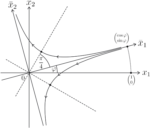
Figure 3: Phase space for the saddlepoint ODE system (7) with sample trajectories and lines where hitting distributions are recorded (dashed lines).

3.2 Theoretical hitting distribution

As discussed in Section 2.2, the numerical solution to the above ODE system undergoes a transition from converging to the actual solution to diverging from it. During this transition, the numerical trajectory crosses one of the straight lines passing through 0 at an angle $\phi\pm\theta$ for each value of $\theta\in(0,\pi/2)$. These intersections are important as they indicate the onset of divergent behaviour. The hitting distributions also provide a means of measuring the random variable $Z_{\infty}$, which drives the random variations in our solutions, and hence of verifying the theoretical results.

Equation (6) gives the asymptotic distribution of the magnitude of the point at which the numerical solution hits the line through the origin at angle $\varphi\pm\frac{\pi}{4}$ as $|Z|^{\frac{\mu}{\lambda+\mu}}$ where $Z$ is a Gaussian random variable with mean 0 and variance

$$\sigma^{2}=h\sigma_{\infty}^{2}=\frac{1}{3(\lambda+\mu)}h2^{-2p}(\cos\varphi\sin\varphi)^{2}$$ (9)

i.e. $Z\sim\mathcal{N}(0,\sigma^{2})$. We obtain an explicit formula for the asymptotic distribution by starting from the $\mathcal{N}(0,\sigma^{2})$ distribution

$$p(x)\text{d}x=\frac{1}{\sqrt{2\pi}\sigma}\exp\Big{(}-\frac{1}{2\sigma^{2}}x^{2}\Big{)}\text{d}x$$

and performing a transformation of the variable given by $y=|x|^{\frac{\mu}{\lambda+\mu}}$. The result is:

$$p(y)\text{d}y=\frac{2(\lambda+\mu)}{\sqrt{2\pi}\sigma\mu}y^{\frac{\lambda}{\mu}}\exp\Big{(}-\frac{1}{2\sigma^{2}}y^{\frac{2(\lambda+\mu)}{\mu}}\Big{)}\text{d}y.$$

In the case $\lambda=\mu=1$ which we shall consider below, setting $a=\frac{4}{\sqrt{2\pi}\sigma}$, we obtain the family of distributions

$$f(x)\text{d}x=ax\exp\Big{(}-\frac{\pi}{16}a^{2}x^{4}\Big{)}\text{d}x$$ (10)

which we shall fit to our numerical data to confirm our theoretical value of $a$.

3.2.1 Choice of parameters

Since there is no random element contained in a deterministic solver, for each repetition at least one parameter has to vary. At first, we tried varying the initial value in the direction of the eigenvectors, but this did not yield any interesting results. The chosen distribution of initial values was reproduced exactly in the hitting distribution and no randomness could be observed. Also, from an aesthetic point of view, it is preferable to vary only ‘internal’, i.e. numerical parameters of an algorithm, such as the time step size or error tolerances, instead of varying ‘physical’ parameters of the system like the initial value.

The only internal parameter of Euler’s algorithm is the time step size $h$, which we varied as follows. Given a user-supplied value of $h$, the step size $h_{i}$ for the $i^{\text{th}}$ repetition ($i\in\{1,\dots,L\}$) is defined by

$$h_{i}=h+\Delta h(i-1-k),$$

where the number of repetitions $L=2k+1$ and $0<\Delta h\ll h$ are also user-supplied. For all simulations, we set $k=10^{4}$.

In each run, the trajectory at some point intersects the lines $\bar{x}_{1}=\pm\bar{x}_{2}$ (the dashed lines in Figure 3). In order to produce histograms, we partition the interval $[0,1]$ into a given fixed number of subintervals of equal length and count how many times $y$ falls into each subinterval, where $y$ denotes the distance of the point of intersection from the origin.

Since the limit distribution is given by $|Z|^{\frac{\mu}{\lambda+\mu}}$, if the values of $\lambda$ and $\mu$ differed significantly then the distribution would be hard to observe in a numerical experiment. Furthermore, if $\lambda\gg\mu$ then the trajectories are very quickly pushed away from the $\bar{x}_{1}$-axis so that fluctuations (i.e. rounding errors) become largely irrelevant. Conversely, if $\mu\gg\lambda$ then the amplification of deviations from the $\bar{x}_{1}$-axis is too weak to be observable. These arguments suggest choosing $\lambda$ and $\mu$ within the same order of magnitude, and we therefore chose $\lambda=\mu=1$ for all simulations.

Another subtlety concerns the choice of the rotation angle $\varphi$. For certain values, trivial trajectories or symmetry effects can occur which conceal the desired accumulation of rounding errors. For instance, for $\varphi=0$ the second component $\bar{x}_{2}$ of the solution is always zero, and therefore the trajectory stays on the line $\bar{x}_{2}=0$ (or equivalently $x_{2}=0$) with no fluctuations. Note that this is in agreement with $\sigma^{2}=0$ in equation (9). For $\varphi=\pi/4$, any rounding error that appears in one component also appears in the other one, which implies that, again, the trajectory always stays on the line $\bar{x}_{2}=0$ (or equivalently $x_{1}=x_{2}$). This case is pathological as it consistently violates our assumption that the rounding errors are independent for each component. For these reasons, we chose $\varphi=\pi/5$ throughout.

Reasonable choices of $h$ and $\Delta h$ are limited by several factors. If $h$ is too large (in the considered case $h>10^{-1}$ for both single and double precision) then the observed hitting distributions differ substantially from the theoretical one because not enough rounding errors can accumulate and hence the deviations are not sufficiently random. The onset of such effects can be seen for large values of $h$ in Figure 6. Lower bounds on $h$ are imposed on the one hand by computational cost and on the other hand by the numerical accuracy of the computer on which the calculations are performed. In practice, however, computational expense becomes prohibitive for values of $h$ much larger than the smallest values permitted by numerical accuracy. Our particular choice of step size distribution requires that $k\Delta h$ should be (much) smaller than $h$. The lower limit for $\Delta h$ is determined solely by the numerical precision, i.e. $\Delta h/h$ must not be smaller than the numerical precision because otherwise there is no variation at all and hence no randomness.

It is beyond the scope of this paper to investigate in detail the dependence of our observations on the distribution of step sizes. However, preliminary experiments with varying $\Delta h$ and even with non-uniform step size distributions suggest that this dependence is very weak for a wide range of conditions. The mean value of the step size distribution, whose effect on the shape of the hitting distribution (i.e. the parameter $a$ in equation (10)) has been demonstrated in Figure 6, seems to be most significant. On the other hand, the variance seems irrelevant apart from being large enough to produce randomness, and does not affect the parameter $a$. This is also supported by the fact that $a$ is (asymptotically) independent of the number of repetitions $L$.

Figure 4 shows that the shape of the distribution exhibits no discernible systematic dependence on $\Delta h$ over at least nine orders of magnitude. This reinforces that the parameter $a$ is unaffected by the variance of the step size distribution for this particular case. The deviations seen for values of $\Delta h$ smaller than about $10^{-19}$ are due to the fact that $\Delta h/h$ approaches the limits of numerical precision.

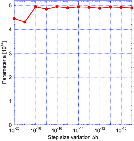
Figure 4: Step size variation for Euler’s algorithm (double precision, step size $h=10^{-4}$, $L=20001$ repetitions each).

3.2.2 Results and observations for explicit methods

Using the given values, distributions as shown in Figure 5 are obtained. We fitted the theoretical distribution (10) to the ones produced numerically with very good agreement.

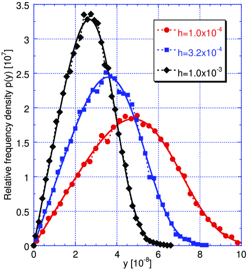
Figure 5: Observed hitting distributions with theoretical fits for Euler’s algorithm ($\Delta h=10^{-10}$, $L=20001$ repetitions each).

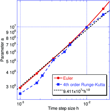
(a) Single precision ($\Delta h=10^{-8}$).

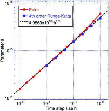
(b) Double precision ($\Delta h=10^{-10}$).

Figure 6: Parameter $a$ in equation (10) as function of the time step size $h$ for simple explicit methods (Euler and $4^{\text{th}}$ order Runge-Kutta).

From the numerical experiments we obtain for each $h$ a distribution of the form (10), where the parameter $a$ is given as a result of the fitting procedure. In Figure 6 the parameter $a$ is plotted as a function of the time step size $h$, both for single (Figure 6(a)) and double (Figure 6(b)) precision ($4$ and $8$ bytes internal representation of floating point numbers respectively). Error bars due to the fit are only about $1\%$ and hence invisibly small. In both cases, the dependence between $a$ and $h$ seems to be well described by $a\propto\sqrt{h}$. Intuitively, one might explain the qualitative behaviour as follows: The smaller the step size, the more numerical errors accumulate, and hence the broader the distribution. The intuition “the smaller the step size, the higher the accuracy, and hence the narrower the distribution”, although at first sight equally valid, is false. In the single precision case, because of the lower accuracy compared to double precision, the distributions are much broader for a given step size.

Equation (9) predicts the value of $ah^{-\frac{1}{2}}$ to be

$$ah^{-\frac{1}{2}}=\frac{4\sqrt{3}}{\sqrt{\pi}\cos\frac{\pi}{5}\sin\frac{\pi}{5}}\times 2^{p}=8.220\times 2^{p}.$$

For Euler’s method, the above data give $ah^{-\frac{1}{2}}=9.411\times 10^{7}$ for single precision and $ah^{-\frac{1}{2}}=4.956\times 10^{16}$ for double precision. For $4^{\text{th}}$ order Runge-Kutta, the values are $ah^{-\frac{1}{2}}=9.27\times 10^{7}$ (with a relatively large error of $\pm 0.12\times 10^{7}$) for single precision and $ah^{-\frac{1}{2}}=4.746\times 10^{16}$ for double precision. Using the approximation discussed in Section 2.2, the actual value of $p$ is between 23 and 24, when working in single precision, and between 52 and 53 when working in double precision, the particular value depending on the exact number being computed. Our theoretical results therefore predict $ah^{-\frac{1}{2}}$ lies between $6.895\times 10^{7}$ and $1.379\times 10^{8}$ for single precision and between $3.702\times 10^{16}$ and $7.404\times 10^{16}$ for double precision.

There are three possible sources of error in our calculations. The first is the error in fitting the numerical data to the theoretical model, the second is that our theoretical models are based on asymptotic results as $h\rightarrow 0$, whereas we are applying them to values of $h$ which are necessarily larger than the precision of the computer. The third source of error arises from the assumption that at each stage the rounding error can be viewed as an independent uniform random variable, depending on a fixed value of $p$. The above results show the above errors are all small and our theoretical model provides a very good fit.

3.2.3 Implicit solvers

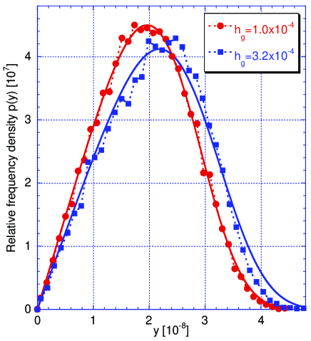
Figure 7: Hitting distributions for VODE.

Possible internal parameters to be varied in solver packages more sophisticated than Euler’s method are typically the error tolerances RTOL (relative) and ATOL (absolute) and the global time step $h_{\text{g}}$ (the time interval after which the user requests solution output from the solver). However, naturally the user has no immediate control over the size of the actual steps taken, which is determined algorithmically as a function of the error tolerance parameters RTOL and ATOL, frequently by trial-and-error methods using heuristics, but only rarely by an explicit formula. Nonetheless, as shown in Figure 7, distributions very similar to the ones seen for Euler’s algorithm (Figure 5) can be generated. Experiments do not readily suggest a simple relationship between the shape of the distribution (parameter $a$ in equation (10)) and any of the parameters ATOL, RTOL, and $h_{\text{g}}$. We suspect the lack of direct control over the time step size to be the main reason for this behaviour. We found that in order to produce Figure 7, one has to use $\texttt{RTOL}=0$, which we also attribute to the step adaptation.

For the solver RADAU5 [6] the results are qualitatively similar, which supports the assertion that the observed phenomena are not specific to a particular algorithm, but rather general effects.

4 Conclusion

We analysed the cumulative effect of rounding errors incurred by deterministic ODE solvers as the step size $h\rightarrow 0$. We considered in particular the interesting case where the ordinary differential equation has a saddle fixed point and showed that the numerical solution is inherently random and also obtained its theoretical distribution in terms of the time, step size and numerical precision. We showed that as the step size $h\rightarrow 0$, the numerical solution exhibits three types of behaviour, depending on the time: initially it converges to the actual solution, it then undergoes a transition stage, finally it diverges from the actual solution.

By performing multiple repetitions with different values of the time step size, we observed the random distributions predicted theoretically. We demonstrated that during the transition period described above the numerical solution intersects all the straight lines through the origin. The theoretical and numerical distributions for the points at which these intersections occur showed very good agreement. Both the mean and the standard deviation of these distributions were found to be of the form $ah^{\gamma}$, where $\gamma\in(0,1/2]$ is a constant determined by the ODE system, and $a$ was found explicitly in terms of the precision of the computer. We mainly focused on the explicit Euler and RK4 methods, however, we also briefly considered the implicit solvers VODE and RADAU5 to demonstrate that the observed effects are not specific to a particular numerical method.

Acknowledgments

This work has been partially funded by the EPSRC (grant number GR/R85662/01) under the title “Mathematical and Numerical Analysis of Coagulation-Diffusion Processes in Chemical Engineering”. The authors thank James R. Norris and Markus Kraft for suggesting the project and the collaboration, and helpful discussions.

Sebastian Mosbach
Department of Chemical Engineering
University of Cambridge
Pembroke Street
Cambridge
CB2 3RA
UK
E-mail: sm453@cam.ac.uk

Amanda Turner
Statistical Laboratory
Centre for Mathematical Sciences
Wilberforce Road
Cambridge
CB3 0WB
UK
E-mail: A.G.Turner@statslab.cam.ac.uk

References

- [1]
- [2] P. N. Brown, G. D. Byrne, and A. C. Hindmarsh. VODE, a variable-coefficient ODE solver. SIAM Journal on Scientific and Statistical Computing, 10(5):1038–1051, 1989.
- [3] J. R. Cash. Efficient numerical methods for the solution of stiff initial-value problems and differential algebraic equations. Proc. R. Soc. Lond., 459:797–815, 2003.
- [4] G. E. Forsythe. Reprint of a note on rounding-off errors. SIAM Rev., 1(1):66–67, 1959.
- [5] H. H. Goldstine and J. von Neumann. Numerical inverting of matrices of high order II. Proc. Amer. Math. Soc., 2:188 –202, 1951.
- [6] E. Hairer and G. Wanner. Solving Ordinary Differential Equations II. Stiff and Differential-Algebraic Problems, volume 14 of Springer Series in Computational Mathematics. Springer Verlag, Berlin Heidelberg New York, second revised edition, 1996.
- [7] P. Henrici. Discrete Variable Methods in Ordinary Differential Equations. John Wiley & Sons, New York, 1962.
- [8] P. Henrici. Error Propagation for Difference Methods. John Wiley & Sons, New York, 1963.
- [9] P. Henrici. Elements of Numerical Analysis. John Wiley & Sons, New York, 1964.
- [10] P. Henrici. Test of probabilistic models for the propagation of roundoff errors. Comm. ACM, 9(6):409–410, 1966.
- [11] N. J. Higham. Accuracy and Stability of Numerical Algorithms. Society for Industrial and Applied Mathematics, 1996.
- [12] T. E. Hull and J. R. Swenson. Test of probabilistic models for the propagation of roundoff errors. Comm. ACM, 9(2):108–113, 1966.
- [13] IEEE standard for binary floating-point arithmetic, ANSI/IEEE Standard 754-1985. Institute of Electrical and Electronics Engineers, 1985. Reprinted in SIGPLAN Notices, 22(2):9-25, 1987.
- [14] W. H. Press, S. A. Teukolsky, W. T. Vetterling, and B. P. Flannery. Numerical Recipes in C++ The Art of Scientific Computing. Cambridge University Press, Cambridge, 2nd edition, 2002.
- [15] A. G. Turner. Convergence of Markov processes near saddle fixed points. Submitted, 2004. Preprint available at http://uk.arxiv.org/abs/math.PR/0412051
- [16] J. H. Wilkinson. Rounding Errors in Algebraic Processes, volume 32 of Notes on Applied Science. Her Majesty’s Stationery Office, London, 1963. Also published by Prentice-Hall, NJ, USA. Reprinted by Dover, New York, 1994.