Hexagonal Tilings: Tutte Uniqueness
Abstract
We develop the necessary machinery in order to prove that hexagonal tilings are uniquely determined by their Tutte polynomial, showing as an example how to apply this technique to the toroidal hexagonal tiling.
1 Introduction
The main result in this paper has to do with graphs determined by their Tutte polynomial. This is a two variable polynomial associated with any graph , which contains interesting information about . For instance, is the number of acyclic orientations of and with is the chromatic polynomial associated with . As a natural extension of the concept of chromatically unique graph, the notion of Tutte unique graph was studied in [9]. A graph is said to be Tutte unique if implies for any other graph . A common topic in the study of this invariant is the search of large families of Tutte unique graphs. In 2003, Garijo, Márquez, Mier, Noy, Revuelta [7],[8] present locally grid graphs as the first large family of graphs uniquely determined by their Tutte polynomial. In this paper we prove that the toroidal hexagonal tilings also satisfy this uniqueness property. The technique developed here can also be applied to the rest of hexagonal tilings and their dual graphs, the locally graphs. The main motivation for this study is the search of a generalization to locally plane graphs of the well known relationship existing between the Tutte polynomials of plane graphs and their duals [13].
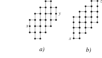
A hexagonal tiling, , is defined as a connected cubic graph of girth 6, having a collection of -cycles, C, such that every path is contained in precisely one cycle of C (path condition). A hexagonal tiling is simple (that is, without loops and multiple edges) and every vertex belongs to exactly three hexagons (cycles of length 6)(Figure 1). Every hexagon of the tiling is called a cell.

Let be a graph with vertex set and edge set . The rank of a subset is , where is the number of connected components of the spanning subgraph . The Tutte polynomial is defined as follows:
contains exactly the same information about as the rank-size generating polynomial which is defined as:
The coefficient of in is the number of spanning subgraphs in with rank and edges, hence the Tutte polynomial tell us for every and the number of edges-sets in with rank and size .
The main strategy in the paper is the following. We first recall some definitions and results from [5, 12], such as, the classification theorem of hexagonal tilings. In Section 3, we show that these graphs are locally orientable, using the relationship existing between hexagonal tilings and locally grid graphs [5]. The local orientation of these graphs allows us to count edge-sets and it is one of the basic tools used to prove the Tutte uniqueness results. Thus, as an example, in Section 5 we apply the technique developed to show that for every hexagonal tiling not isomorphic to with vertices there is at least one coefficient of the rank-size generating polynomial in which both graphs differ.
2 Preliminary Results
In this section we state the classification theorem of hexagonal tilings proved in [5]. There exits an extensive literature on this topic. See for instance the works done by Altshuler [1, 2], Fisk [3, 4] and Negami [10, 11]. In [5], following up the line of research given by Thomassen [12], we add two new families to the classification theorem given in [12] proving that with these families we exhaust all the cases.
Theorem 2.1.
[5] If is a hexagonal tiling with vertices, then one and only one of the following holds:
|
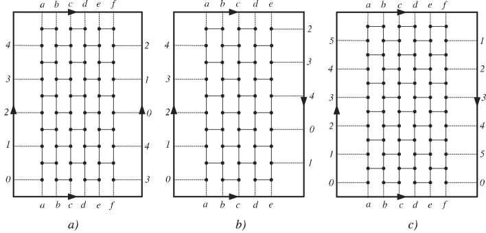
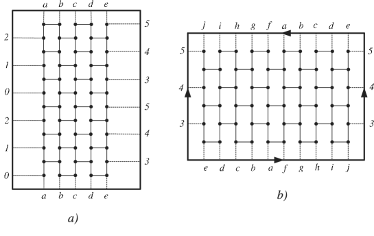
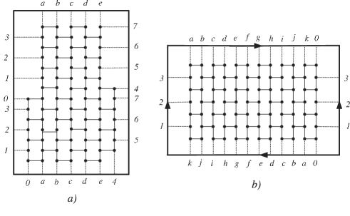
Some examples of hexagonal tilings are given in Figures 2, 3, 4 and 5. The parameters and fix, respectively, the height and the breath of the structures, called hexagonal wall of length and breath (Figures 2, 3, 4) and hexagonal ladder of length and breath (Figure 5), in which it is added edges to construct the different families of hexagonal tilings (see [5]).
Given two cycles and in a hexagonal tiling , we say that is locally homotopic to if there exists a cell, , with connected and is obtained from by replacing with . A homotopy is a sequence of local homotopies. A cycle in is called essential if it is not homotopic to a cell. Otherwise it is called contractible. This definition is equivalent to the one given for a graph embedded in a surface [6]. Let be the minimum length of the essential cycles of , is invariant under isomorphism. An edge-set contained in a hexagonal tiling is called a normal edge-set if it does not contain any essential cycle.
There are two different ways of pasting together ladders each one containing hexagons, from which we obtain two structures, called the ladder and the displaced ladder , shown in Figure 6. Note that the number of shortest paths between and or between and in a ladder or in a displaced ladder is and the length of these paths is .
Every hexagonal tiling is obtained by adding edges to a hexagonal wall or to a hexagonal ladder (except for , in which we have also added two vertices) [5]. These edges are called exterior edges and every essential cycle must contains at least one of these edges ( the edges and in are not considered exterior edges).
3 Local Orientability of Hexagonal Tilings
In this section we prove that hexagonal tilings are locally orientable. This fact allow us to count edge-sets and it is the tool to distinguish at least one coefficient of the Tutte polynomials associated to two non isomorphic hexagonal tilings. We first recall a minor relationship existing between hexagonal tilings and locally grid graphs (see [5]).
We say that a regular, connected graph is a locally grid graph if for every vertex there exists an ordering of and four different vertices , such that, taking the indices modulo 4,
|
|
and there are no more adjacencies among than those required by this condition (Figure 7).

Every locally grid graph is a minor of a hexagonal tiling and in [5] it was proved that there exits a biyective minor relationship preserved by duality between hexagonal tilings with the same chromatic number and locally grid graphs. A perfect matching is selected in each one of the families given in the classification theorem of hexagonal tilings, except in one case, in which the set of selected edges is not a matching. contains two edges of each hexagon. In there are hexagons in which we select four edges pairwise incident. A locally grid graph is obtained by contracting the edges of this matching, and deleting parallel edges if necessary. There are just two cases in which parallel edges must be deleted, and . These perfect matchings and the set of edges of verify that if we have two hexagonal tilings with the same chromatic number, the result of the contraction of their perfect matchings (or the selected edges in ) are two locally grid graphs belonging to different families. This condition is going to be essential in the search of a generalization, for these families, of the relationship existing between the Tutte polynomial of a plane graph and its dual [13].
In [8] it was proved that locally grid graphs are locally orientable. Given a vertex of a locally grid graph , two edges incident with are said to be adjacent if there is a square containing them both; otherwise they are called opposite. An orientation at a vertex consists of labeling the four edges incident with bijectively with the labels , , , in such a way that the edges labelled and are opposite, and so are the ones labelled as and .
Lemma 3.1.
Hexagonal tilings are locally orientable.
Proof.
Let be a hexagonal tiling. By Theorem 2.1, is isomorphic to one of the following graphs: , , , , , , .
Suppose first that is not isomorphic to . For every vertex there is exactly one edge of the perfect matching incident with , call it . Consider the union of the local structures of and , labeling the other two edges incident with as and and the other two edges incident with as and . Contract all the edges of belonging to this union, deleting parallel edges if necessary. As it is shown in Figure 8a we obtain a grid , hence we can label the edges , , and bijectively with the labels , , , following the criterion established for the locally grid graphs. The edge is considered opposite to the unique edge incident with and belonging to the perfect matching, , formed by the edges , not belonging to .
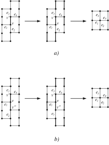
If is isomorphic to , then there are either one or two edges belonging to and incident with . If does not belong to a hexagon that has more than two edges of , we follow the same process as in the previous case. Suppose, now, that is a vertex belonging to one of the hexagons that contains four edges belonging to . We consider two cases:
(1) There are two edges of incident with , call them and . The union of the hexagonal structures of , and is composed by five hexagons. Label the unique edge incident with and not belonging to as . The edge incident with not belonging to and sharing an hexagon with is labelled . Finally, the edges incident with no belonging to are labelled and . Contracting all the edges of belonging to this union and deleting parallel edges, we also obtain a grid and we can label the edges incident with , and bijectively with the labels , , , (Figure 8b). and are considered opposite to the unique edge incident with and respectively, belonging to .
(2) There is one edge of incident with , call it . There has to be one edge, different from , incident with and belonging to , call it . The union of the hexagonal structures of and is composed by five hexagons. The two edges incident with not belonging to are labelled and . The unique edge incident with not belonging to is labelled , and the edge incident with not belonging to or to the hexagon that contains four edges of , is labelled . Contracting all the edges of belonging to this union and deleting parallel edges, we also obtain a grid and we can label the edges incident with , and bijectively with the labels , , , . and are considered opposite to the edges incident with and respectively, belonging to the hexagon that contains four edges of .
∎
The previous proof give us a definition of adjacent and opposite edges for hexagonal tilings. Two edges incident with a vertex and no belonging to are called adjacent or opposite if they are so in the locally grid structure resulting from applying the operations explained above. Two edges incident with and belonging to are always opposite.
By the orientation we mean that is the origin vertex, , is the unique edge incident with and opposite to the other two edges incident with . This edge never belongs to and it is labelled . Finally, is an edge incident with and labelled . The orientation means that is the origin vertex, , is the unique edge incident with and opposite to the other two edges incident with , and is an edge incident with labelled . We will denote both cases as .
If , we denote the label opposite to . If we fix an orientation at ( is the origin vertex) then every vertex adjacent to is unambiguously oriented, because the orientation at induces an orientation at : if is labelled from , it is labelled from . If is a hexagon and , are labelled and from respectively, then is from , is from , is from and is from . We also can translate the orientation at to all the vertices of a path beginning at , but two different paths joining and can induce different orientation at . This does not happen if the union of these two paths is a contractible cycle. In fact, we can transform one path into the other one using three elementary transitions and their inverse: if , , , , , are the edges of a hexagon ordered cyclically, we can change , , , , by ; , , , by , and , , by , , and these operations do not change the orientation at the endpoint.
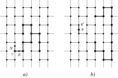
Let be a connected normal edge set in a hexagonal tiling . Fixed an orientation at a vertex , then all the vertices in are unambiguously oriented. Every path in can be described as a sequence of the labels (Figure 9a). This allow us to assign coordinates to every vertex in : has coordinates and has coordinates if in one path in joining to (taking into account that the orientation at the endpoint induced by different paths joining to does not change), is the number of labels minus the number of labels and is the number of labels minus the number of labels .
Lemma 3.2.
Let be a connected normal edge set in a hexagonal tiling with , then different vertices in have different coordinates.
Proof.
First, we are going to prove that with a fixed orientation no vertex except the origin can have coordinates . Suppose that there exists such that has coordinates , then there exits a path joining to with as many labels as labels and as many labels as labels . We are going to show that by induction on the length of this path.
If and is the origin vertex, the first labels of can be: , , , , or and using the elementary transitions described previously, we can change these labels by , , , and respectively. To obtain as many labels as labels and as many labels as labels it must be that . We assume that every path (not a cycle) with does not have as many labels as labels and as many labels as labels and we prove the result for . Suppose that there exits a path joining and , not a cycle, with and having as many labels as those labelled and as many as , then there exits a subsequence labelled or (or other analogous subsequence). In the first case we can change this subsequence by keeping the orientation at the endpoint. Analogously, in the second case the subsequence can be changed by . In any case, the change gives rise to a new path joining and with , in a new connected edge set . This set is also a normal edge set because . By hypothesis, does not have as many labels as and as , hence neither does and we obtain a contradiction.
Given two different vertices, and in , we consider the paths and joining to and to respectively. Since is connected, there is a path joining to and keeping the orientation at . Hence, it is easy to prove that and can not have the same coordinates. ∎
From now on, and unless otherwise stated, we consider that all normal edge-sets have at most elements.
4 Counting Edge-Sets
The aim of this section is to find a system which allow us to count edge-sets in order to prove that there is at least one coefficient of the rank-size generating polynomial in which two non isomorphic hexagonal tilings differ. Our first step is to codify the edge-sets of a hexagonal tiling.
Let be the infinite plane square lattice, that is, the infinite graph having as vertices and in which is joined to . We delete the edges if even and if odd, obtaining a infinite plane hexagonal tiling . Let be the group of graph automorphisms of . This group is generated by translations, symmetries and rotations of the plane that map vertices to vertices. Let be the set of all finite connected edge-sets of . An equivalence relation is defined in as follows:
If is a set of representatives of such that every contains the vertex , then covers all the possible shapes that a normal edge-set could have.
We are going to define a set of words over the alphabet that represents all edge- sets of . Label as , as , from as and as . For every there is a sequence over the the alphabet such that beginning at and following the instructions given by the unique edges covered are those of . Note that one edge can be covered more than once and that the sequence is not unique (Figure 9a). Since every sequence over the alphabet can not represent a set of (for instance, a sequence with two consecutive labels ) we are going to establish some restrictions on this alphabet:
(1) No sequence begins with the label .
(2) There are no two consecutive labels (analogously ).
(3) If a sequence begins with a label (analogously ), there must be an odd number of labels and before having a label ; and an even number if the label is . Hence, there are an odd number of labels and between two labels and an even number between two labels .
(4) If a sequence begins with a label , there are an odd number of labels and between two labels and an even number between two labels .
Call the set of words over the alphabet verifying the three previous conditions. These restrictions do not modify the fact that every has a word associated. Conversely, given there exits , such that . It will be denoted .
The next step is to assign one word from to each normal connected edge-set of a hexagonal tiling, . Fix an orientation at , being the origin vertex. Following the code given by from with orientation , an edge set is obtained, called the instance of in and we call an orientation of the instance. An instance of can have different orientations associated to it, the number of them depends only on the symmetries of and it is called . The length of is the number of labels , , , that give rise to .
Lemma 4.1.
Let be a hexagonal tiling and . If and , then is a normal edge-set and it has the same rank and size as .
Proof.
We are going to prove this result by induction on the length of . If has length equal to one, the result is trivial. Let be the word resulting from removing the last label from . By hypothesis is normal and it has the same rank and size as . When we add the last label of to , there are three possibilities on :
(1) We are adding one edge between two vertices belonging to
(2) We are adding an isthmus.
(3) We do not add any edge.
(1) Let be the last vertex of covered by . Since is normal all the vertices of are unambiguously oriented. Let be the added edge. This edge is labelled from following the orientation . Suppose that is not a normal edge-set, then when we have added the edge we have created an essential cycle. Since , has to be an essential cycle. contains at least one cycle because it has been obtained joining two vertices of . Hence contains a subword that can be , , (or other analogous cases to the last ones) (Figure 9b). We change these subwords by , , respectively.
In any case, a word is obtained of length smaller than the length of , hence is a normal edge-set and contains a cycle. If we consider the simply connected region determined by and we add, depending on the case, one hexagon or two columns of hexagons, a simply connected region is obtained which is determined by . Since is an essential cycle, at least one vertex of the added hexagons belongs to . Therefore, has at least two cycles and we obtain a contradiction. The equality of ranks and sizes remains to be proved. By hypothesis of induction and . Furthermore and . Since is normal, and .
(2) and (3) The second case is easier than the previous one. Using a similar reasoning we obtain that if is not a normal edge-set, then it is an essential cycle. But an essential cycle only could be created joining two vertices belonging to . The equality of ranks and sizes is proved as in case (1). The third case is trivial because if we do not add any edge, . ∎
Lemma 4.2.
Let be a connected normal edge-set. Fixed an orientation with , there exits a unique edge-set and a unique graph isomorphism such that:
(1) .
(2) If the edge is labelled from , then is labelled from according to the orientation .
Proof.
Fixed an orientation with , we can assign coordinates to the vertices of . Since is normal, this assignment is unambiguous. We define by if in every path in joining to , is the number of labels minus the number of labels and is the number of labels minus the number of labels . Furthermore, we define by . Taking , it is easy to prove that is a graph isomorphism and that is the isomorphism induced on edges by . The statements (1) and (2) of the lemma are consequence of the assignment of coordinates following an orientation in a hexagonal tiling , and the assignment of labels in the edges incident with the origin vertex . We prove the uniqueness of by induction on max. Suppose that there exits a pair verifying the statement of the lemma. If , with hence . By (1) and (2), it is immediate to show that . Assume the result for and we prove it for . There exits such that and for all . By induction on we show that is unique for . If , let be the unique vertex such that and let be the set of edges incident with and belonging to . Call the connected normal edge-set resulting from deleting the vertex . By the induction hypothesis, there exits a unique pair associated to , then . Suppose that is unique for and having vertices such that . Using the same argument as in the previous case, it is easy to prove the result for vertices. ∎
Using the same arguments as those given in [8] for locally grid graphs, we prove the following result.
Lemma 4.3.
Given a connected normal edge-set , there exits a unique word and an orientation , not necessarily unique, such that .
Lemma 4.4.
For fixed , the number of connected normal edge-sets with rank and size is the same for all hexagonal tilings with vertices and such that .
Proof.
By the previous lemma, every connected normal edge-set is the instance of a unique word . By Lemma 4.2 is isomorphic to then they have the same rank and size. By Lemma 4.1 the instance of a word is a normal connected edge-set. Hence, the number of connected normal edge-sets with rank and size is equal to the number of distinct instances of words corresponding to edge-sets of with rank and size . For every fixed we can choose different orientations. Let be the set of words of such that and . Then the number of connected normal edge-sets with rank and size is:
Since depends only on the word, this quantity does not depend on the graph. ∎
A non-connected version of this lemma is proved for hexagonal tilings as in [8] for locally grid graphs.
Lemma 4.5.
For fixed and , the number of normal edge-sets with rank , size and connected components is the same for all hexagonal tilings with vertices and such that .
Lemma 4.6.
Fix . The number of edge-sets with rank and size that do not contain essential cycles is the same for all hexagonal tilings with vertices and such that .
Corollary 4.7.
Let , be a pair of hexagonal tilings with vertices.
implies .
If but and do not have the same number of shortest essential cycles then .
Proof.
If , there are essential cycles of length in but not in . Since by the preceding lemma the number of normal edge-sets with rank and size is the same in and , the coefficient of in the rank-size generating polynomial is greater in than in . In a analogous way the second statement is proved. ∎
The process we have followed to count normal edge-sets of size smaller than , is to show that we can assign a unique set, to every normal edge-set, . Our next aim is to prove that for some special cases we can count normal edge-sets with size greater than . This fact is going to be essential in the next section. Denote by the number of normal edge-sets in with rank , size and having as a subgraph. An edge-set is a forbidden edge-set for if it contains an essential cycle and a subset isomorphic to .
Corollary 4.8.
Given such that contains at least one cycle, then we have that is the same for all hexagonal tilings with vertices, with no forbidden edge-set for of size and such that .
Proof.
Fix such that contains at least one cycle. We just have to prove that given such that , and , then is a normal edge-set and it has the same rank and size as . This result is analogous to Lemma 4.1 but taking size smaller than .
If then contains at least one cycle. If , the proof is equal to the one for Lemma 4.1. If , we show that has to be an essential cycle (then the rest of the proof would be analogous to the one followed in Lemma 4.1). Suppose that contains an essential cycle and one more edge. Since:
then is a forbidden edge-set for of size and we obtain a contradiction. The cases in which and are analogously proved. ∎
5 Tutte Uniqueness
In this section we apply the results obtained in order to prove the Tutte uniqueness of . First we are going to show that the local hexagonal tiling structure is preserved by the Tutte polynomial, using the following lemmas.
Lemma 5.1.
[5] The edge-connectivity of every hexagonal tiling is equal to three.
Lemma 5.2.
[9] If is a connected simple graph and is Tutte equivalent to , then is also simple and connected. If is a connected simple graph, then the following parameters are determined by its Tutte polynomial:
(1) The number of vertices and edges.
(2) The edge-connectivity.
(3) The number of cycles of length three, four and five.
Next, we are going to prove that there is at least one coefficient, in which, the Tutte polynomial associated to and the Tutte polynomial associated to any other hexagonal tiling not isomorphic to , differ. As we have explained in the first section, the Tutte polynomial associated to a graph tell us for every and the number of edges-sets in with rank and size . There are two different types of these edge-sets: normal edge-sets (do not contain essential cycles) and edge-sets containing at least one essential cycle. We recall two results from [5]
Lemma 5.3.
[5] Let be a hexagonal tiling, then the length of their shortest essential cycles and the number of these cycles is:
|
|
Lemma 5.4.
[5] If is one of the hexagonal tilings, then the chromatic number of is given in the following table:
|
Theorem 5.5.
Let be a graph Tutte equivalent to a hexagonal tiling , then is an hexagonal tiling.
Proof.
By Theorem 2.1 and Lemma 5.1 , we know that has vertices for some , , edges and edge-connectivity equal to three. By Lemma 5.2, has the same parameters, so is cubic, has vertices and edges. Since is a hexagonal tiling, has girth six hence from the previous lemma, has girth at least six.
In order to prove that is a hexagonal tiling, we must show one more thing: that both graphs have the same number of cycles of length six (hexagons). Since and are Tutte equivalent, they have the same number of edge-sets with rank five and size six. We are going to prove that these sets are cycles of length six.
Let be an edge-set with rank five and size six. If is the number of connected components of , then . Suppose that is not a cycle, since the girths of and are at least six we have where is a connected component of . Hence and we obtain a contradiction. ∎
Theorem 5.6.
The graph is Tutte unique for and .
Proof.
Let be a graph with . By Theorem 2.1 and Lemma 5.4, has to be isomorphic to one and only one of the following graphs: , , , . We prove that is isomorphic to with and by assuming that is isomorphic to each one of the previous graphs and by obtaining a contradiction in all the cases except in the aforementioned case. By Lemma 4.7, we obtain and the number of shortest essential cycles has to be the same in both graphs. The process we follow is to compare with all the graphs given in the previous list. In the cases in which the minimum length of essential cycles or the number of cycles of this minimum length are different, we would have that the pair of graphs compared are not Tutte equivalent. For the sake of brevity, we are only going to show those cases in which these quantities can coincide.
Case 1. Suppose with , and .
As a result of Lemma 4.7, and . Our aim is to prove that the number of edge-sets with rank and size is different for each graph. This would lead to a contradiction since this number is the coefficient of of the rank-size generating polynomial. If has essential cycles of length , then has such cycles, therefore if we show the existence of a bijection between the corresponding edge-sets with rank and size that are not essential cycles, we would have proved the desired result.
For every with , the set of edges that join a vertex to is denoted . Let be an edge-set that is not an essential cycle with rank and size in . Define as min ; . The minimum always exits for all edge-set contained in or that is not an essential cycle. For every with we define the bijection, between and as follows:
If , where
Case 2. Suppose with and .
The arguments to prove that both graphs do not have the same Tutte polynomial are analogous to those developed in the preceding case. We only want to specify two things. The first one is the number of essential cycles of length in each graph, and the second one, is the bijection between the edge-sets with rank and size that are not essential cycles contained in each graph.
In we have exterior edges giving rise to displaced ladders with and . On the other hand, in each of the exterior edges determine a displaced ladder for odd or if is even. Hence, making use of the following property:
the number of essential cycles of length in is smaller that in .
For every we define between and as follows:
If , where
Case 3. Suppose with and .
As in the previous case, we prove that the number of essential cycles of length in is smaller than that in .
For every , the bijection between and is defined as follows:
If , where
Case 4. Suppose with and .
By Lemma 4.7, and . We are going to prove that there are more edge-sets with rank and size in than in . These sets can be classified into three groups:
1.- Essential cycles of length .
2.- Normal edge-sets (they are edge-sets that do not contain any essential cycle).
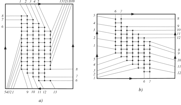
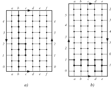
3.- Sets containing an essential cycle of length and three more edges (Figure 10).
(1) Since and are bipartite, they do not have any essential cycle of odd length.
(2) By Corollary 4.8 we know that and have the same number of normal edge-sets with rank and size that do not contain a cycle of length six. We are going to prove that the number of normal edge-sets with rank and size containing a cycle of length six is greater in than in .
Again by Corollary 4.8 , the number of edge-sets with rank and size containing a hexagon is the same in both graphs, call it . Add one edge to each of these sets in order to obtain a set with rank and size . This set can be one of the following types depending on which edge we are adding:
(A) A normal edge set with rank .
(B) A normal edge set containing two non essential cycles and having rank .
(C) A edge set containing an essential cycle of length and a cycle of length six.
Let , and (where is or ) be the number of edge-sets in that belong to the groups A, B and C respectively. is the number of possibilities of adding one edge to the edge-sets with size containing a hexagon and such that the added edge does not belong to a fixed hexagon.
Now, we are going to show that , where is the number of edges of which do not belong to all cycles of length six in . In order to obtain an edge-set we add one edge to an edge-set with size that contains one hexagon, forming a new contractible cycle. Since the cycle is contractible, we can consider that the added edge has to belong to a new hexagon. Hence:
If we apply Corollary 4.8 to every , the number of normal edge-set of size is equal in and then:
Altogether and by taking in account that and (Figure 10) we have proved that .
(3) In , every essential cycle of length plus three edges has rank (Figure 10a), but in there are essential cycles in which if we add three edges we obtain sets with rank (Figure 10b). By hypothesis, both graphs have the same number of shortest essential cycles therefore the number of edge-sets in this case is greater in than in .
Cases 5 and 6 If with and or with we use the same arguments as those in the previous case to prove that has more edge-sets with rank and size than and . ∎
6 Concluding Remarks
We have proved that the toroidal hexagonal tiling, is Tutte unique. Since the results given in Sections 3 and 4 are proved for all hexagonal tilings, it seems that all hexagonal tilings are Tutte unique. To verify this, we would have to do all cross-checkings between any two of these graphs as was done in Section 5. This study has been done for locally grid graphs in [7].
The technique developed in this paper can also be applied to locally graphs. This would follow from the local orientation existing in these graphs, based on the minor relationship described in [5] between locally grid graphs and locally graphs.
References
- [1] A. Altshuler, Hamiltonian Circuits in some maps on the torus, Discret Math. 1(1972), 299-314.
- [2] A. Altshuler, Construction and enumeration of regular maps on the torus, Discret Math. 4(1973), 201-217.
- [3] S. Fisk, Geometric coloring theory, Advances in Math. 24(1977), 298-340.
- [4] S. Fisk, Variations on coloring, surfaces and higher dimensional manifolds , Advances in Math. 25(1977), 226-266.
- [5] D. Garijo, I. Gitler, A. Márquez and M.P. Revuelta, Hexagonal tilings and Locally graphs, Preprint, 2004.
- [6] D. Garijo, Polinomio de Tutte de Teselaciones Regulares, Thesis (2004).
- [7] D. Garijo, A. Márquez and M.P. Revuelta, Tutte Uniqueness of Locally Grid Graphs, Ars Combinatoria (to appear) (2005).
- [8] A. Márquez, A. de Mier, M. Noy, M.P. Revuelta, Locally grid graphs:classification and Tutte uniqueness, Discr. Math. 266 (2003), 327-352.
- [9] A. de Mier, M. Noy, On graphs determined by their Tutte polynomials, Graphs Combin. 20 (2004), no.1, 105-119.
- [10] S. Negami, Uniqueness and faithfulness of embedding of toroidal graphs, Discrete Math. 44(1983), no.2, 161-180.
- [11] S. Negami, Classification of 6-regular Klein bottle graphs, Res. Rep. Inf. Sci. T.I.T.A-96 (1984).
- [12] C. Thomassen, Tilings of the Torus and the Klein Bottle and vertex-transitive graphs on a fixed surface, Trans. Amer. Math. Soc. 323(1991), no.2, 605-635.
- [13] W.T. Tutte Graph Theory, Addison Wesley, California (1984).