Hexagonal Tilings and Locally $C_{6}$ Graphs

Abstract

We give a complete classification of hexagonal tilings and locally $C_{6}$ graphs, by showing that each of them has a natural embedding in the torus or in the Klein bottle (see [12]). We also show that locally grid graphs, defined in [9, 12], are minors of hexagonal tilings (and by duality of locally $C_{6}$ graphs) by contraction of a particular perfect matching and deletion of the resulting parallel edges, in a form suitable for the study of their Tutte uniqueness.

1 Introduction

Given a fixed graph $H$, a connected graph $G$ is said to be locally $H$ if for every vertex $x$ the subgraph induced on the set of neighbours of $x$ is isomorphic to $H$. For example, if $P$ is the Petersen graph, then there are three locally $P$ graphs [7]. In this paper we classify two different families of graphs, hexagonal tilings and locally $C_{6}$ graphs.

We first describe all the necessary structures to obtain the classification of hexagonal tilings, such as the hexagonal cylinder, hexagonal ladder, twisted hexagonal cylinder etc. Some of these structures appear in [12] in an attempt of classification of these graphs. There exits an extensive literature on this topic. See for instance the works done by Altshuler [1, 2], Fisk [4, 5] and Negami [10, 11]. We also want to note Ref. [8] where locally $C_{6}$ graphs appear in an unrelated problem. In this paper, following up the line of research given by Thomassen [12], we add two new families to the classification theorem given in [12] and we prove that with these families we exhaust all the cases. In order to distinguish the families of hexagonal tilings we study some invariants of graphs such as the chromatic number, shortest essential cycles and vertex-transitivity. Locally $C_{6}$ graphs are the dual graphs of hexagonal tilings [12], hence the classification theorem of these graphs is obtained from the classification of hexagonal tilings.

Finally, we are interested in relationships existing between hexagonal tilings, locally $C_{6}$ graphs and locally grid graphs. Specifically those properties that can be related to different aspects of the Tutte polynomial. This is a two-variable polynomial $T(G;x,y)$ associated to any graph $G$, which contains a considerable amount of information about $G$ [3]. A graph $G$ is said to be Tutte unique if $T(G;x,y)=T(H;x,y)$ implies $G\cong H$ for every other graph $H$. In [6] and [9] the Tutte uniqueness of locally grid graphs was studied. We are interested in a similar study for hexagonal tilings and locally $C_{6}$ graphs but in a more unified way, that is in relation to the families of locally graphs that have been Tutte determined.

Informally a locally grid graph is defined as a graph in which the structure around each vertex is a $3\times 3$ grid (a formal definition is given in Section 3). A complete classification of these graphs is given in [9, 12] and they fall into five families. Every locally grid graph is a minor of a hexagonal tiling but we are interested in a biyective minor relationship preserved by duality between hexagonal tilings with the same chromatic number and locally grid graphs. This specific minor relationship is going to be essential in the study of the Tutte uniqueness of hexagonal tilings and locally $C_{6}$ graphs in relation to the Tutte uniqueness of locally grid graphs. In order to obtain this relation we choose for every family of hexagonal tilings obtained in the classification theorem, a specific perfect matching, whose contraction and then deletion of resulting parallel edges (if any) gives rise to a locally grid graph. There is just one family of hexagonal tilings in which the selected edges are not a matching. If we select the set of dual edges associated to the perfect matching (hence on the $C_{6}$ graph), and we delete them and then contract the set of dual edges associated to the parallel edges (if any), we obtain the dual of the locally grid graph, which again is a locally grid graph. These perfect matchings and the set of edges that is not a matching in one of the families verify that if we have two hexagonal tilings with the same chromatic number, the results of the contraction of their perfect matchings (or the set of edges that is not a matching in one of the families) are two locally grid graphs belonging to different families.

Some standard definitions needed along the paper are: A graph is $d-$regular if all vertices have degree $d$. If $d=3$ the graph is called cubic. A $k-$path is a graph with vertices $x_{0},x_{1},\ldots,x_{k}$ and edges $x_{i-1}x_{i}$ with $1\leq i\leq k$. A $k-$cycle is obtained from a $(k-1)-$path by adding the edge between the two ends of the path (vertices of degree one).

2 Classification of hexagonal tilings and locally $C_{6}$ graphs

In this section we give a complete classification of hexagonal tilings, which are connected, cubic graphs of girth 6, having a collection of $6$-cycles, C, such that every $2-$path is contained in precisely one cycle of C ($2-$path condition). In particular, a hexagonal tiling is simple and every vertex belongs to exactly three hexagons (Figure 1). Every hexagon of the tiling is called a cell.

Figure 1: Hexagonal structure around $x$

Let $H=P_{p}\times P_{q}$ be the $p\times q$ grid, where $P_{l}$ is a path with $l$ vertices. Label the vertices of $H$ with the elements of the abelian group $\mathbb{Z}_{p}\times\mathbb{Z}_{q}$ in the natural way. If we add the edges $\{(j,0),(j,q-1)|0\leq j\leq p-1\}$ we obtain a cylinder grid $p\times q$.

A hexagonal wall of length $k$ and breadth $m$ is defined as the graph obtained by removing the edges $\{(2i,2j),(2i+1,2j)\}$ and $\{(2i+1,2j+1),(2i+2,2j+1)\}$ with $0\leq i\leq\lfloor(m-1)/2\rfloor$, $0\leq j\leq k-1$ in a $(m+1)\times 2k$ grid. If we delete the same edges in a cylinder grid $(m+1)\times 2k$ the result is a hexagonal cylinder of length $k$ and breadth $m$ (Figure 2a). The two cycles of this structure, where every second vertex has degree two, are called peripheral cycles. Each one of these cycles has $k$ vertices of degree two labeled as follows: $z_{j}=(0,2j)$ and $x_{j}=(m,2j)$ with $0\leq j\leq k-1$ if $m$ odd, or $z_{j}=(0,2j)$ and $x_{j}=(m,2j+1)$ with $0\leq j\leq k-1$ if $m$ even.

A hexagonal cylinder circuit of length $k$ is a hexagonal cylinder of length $k$ and breadth 1. A hexagonal Möbius circuit of length $k$ is obtained by adding the edges $\{(0,0),(1,2k-1)\}$ and $\{(1,0),(0,2k-1)\}$ to a hexagonal wall of length $k$ and breadth 1. The graph resulting from removing the edges $\{(0,2j+1),(1,2j+1)|0\leq j\leq k-1\}$ and $\{(1,2j),(2,2j)|0\leq j\leq k\}$ in a $3\times(2k+1)$ grid, and adding the edges $\{(0,0),(2,2k)\}$, $\{(1,0),(1,2k)\}$ and $\{(2,0),(0,2k)\}$ is called a parallel hexagonal Möbius circuit (Figure 2b).

Let $H$ be the $(m+1)\times(2k+m)$ grid. A hexagonal ladder of length $k$ and breadth $m$ (Figure 2c) is obtained by removing the following vertices and edges:

$$\{(j,i)|0\leq j\leq m-2,0\leq i\leq m-2-j\}$$

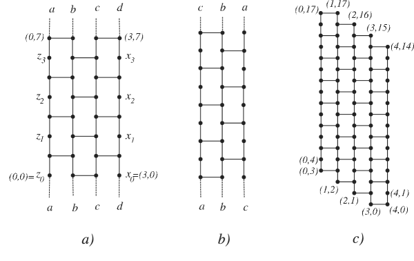
Figure 2: a) Hexagonal cylinder of length 4 and breadth 3 b) parallel hexagonal Möbius circuit of length 9 c) Hexagonal ladder of length $7$ and breadth $4$

From this structure we construct two twisted hexagonal cylinders, $TC_{k,m,1}$ if $k\leq m-2$ (Figure 3b) and $TC_{k,m,2}$ if $k\geq m+1$ (Figure 3a). The first one is obtained by adding two vertices, $(0,2k+m)$ and $(m-k-1,3k+2)$, and the following edges to a hexagonal ladder of length $k$ and breadth $m$: $\{(0,2k+m),(0,2k+m-1)\}$, $\{(0,2k+m),(k+1,m-k-2)\}$, $\{(m-k-1,3k+2),(m-k-1,3k+1)\}$, $\{(m-k-1,3k+2),(m,0)\}$, $\{(j,2k+m-j),(k+j+1,m-k-j-2)\}$ with $1\leq j\leq m-k-2$. $TC_{k,m,1}$ also has two peripheral cycles, $C_{1}$ and $C_{2}$, which contain all the vertices of degree two. In $C_{1}$, they are $z_{j}=(0,2k+m-2j)$ and $x_{j}=(j,m-(j+1))$ with $0\leq j\leq k$. In $C_{2}$, $v_{0}=(m-k-1,3k+2)$, $v_{i+1}=(m-k+1,3k-i)$, $w_{0}=(m,2k)$ and $w_{i+1}=(m,2k-(2i+1))$ with $0\leq i\leq k-1$.

To obtain $TC_{k,m,2}$, we delete the vertices $(m+1,i)$, $0\leq i\leq 2(k-m)-3$ in a hexagonal ladder of length $k$ and breadth $m+1$, and we add the edges $\{(0,2k+m),(m+1,2(k-m-1)\}$ and $\{(0,2k+m-(2j+1)),(m,2(k-m-1)-(2j+2))\}$ with $0\leq j\leq k-m-2$. If $k=m+1$ we do not delete any vertex but we add one edge, $\{(0,2k+m),(m+1,0)\}$. The vertices of degree two of the peripheral cycles, $C_{1}$ and $C_{2}$, are labeled as follows:

$$C_{1}$$: and with .

: and with .

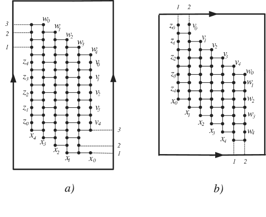
Figure 3: a) $TC_{7,4,2}$ b) $TC_{4,6,1}$

In order to obtain hexagonal tilings, we must adequately add edges between the vertices of degree two in the structures defined above. In the first cases considered below we add the edges between vertices on the peripheral cycles of a hexagonal cylinder. In the last case we add the edges between vertices on the peripheral cycles of a twisted hexagonal cylinder.

From a hexagonal cylinder $H$ of length $k$ and breadth $m$, we obtain the following families of graphs.

A) $H_{k,m,r}$ with $r,k,m\in\mathbb{N}$,   $0\leq r\leq\lfloor k/2\rfloor$, $m\geq 2$, $k\geq 3$. If $m=1$ then $k>3$ and $\lfloor k/2\rfloor\geq r\geq 2$ (Figure 5a).

$$E(H_{k,m,r})=E(H)\cup\{\{z_{j},x_{j+r}\}|0\leq j\leq k-1\}$$

There is a degenerated case, called $H_{k^{\prime},m^{\prime},e}$ in [12], that we want to stress. It is obtained from a cycle of even length $k^{\prime}$ and by adding the adyacencies $\{z_{i},z_{i+m}\}$ taking indices modulo $m$ and taking into account the $2-$path condition, that is, if $z_{i}$ is adjacent to $z_{i+m}$ then $z_{i+1}$ is joined to $z_{l}$ with $l\equiv(i+1)({\rm mod}\,m)$ and $l\neq i+m+1$. This graph is a kind of hexagonal spiral and it is the degenerate case $H_{(k^{\prime}/2),0,m}$ (Figure 4).

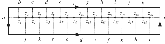
Figure 4: $H_{10,0,5}$

B) $H_{k,m,a}$ with $m\geq 2$,   $k\geq 3$ (Figure 5b).

$$E(H_{k,m,a})=E(H)\cup\{\{z_{0},x_{1}\},\{z_{1},x_{0}\},\{z_{i},x_{k+1-i}\}|2\leq 1\leq k-1\}$$

C) $H_{k,m,b}$ with $k$ even, $m$ odd,   $m\geq 3$,   $k\geq 4$ (Figure 5c).

$$E(H_{k,m,b})=E(H)\cup\{\{z_{0},x_{0}\},\{z_{i},x_{k-1}\}|1\leq i\leq k-1\}$$

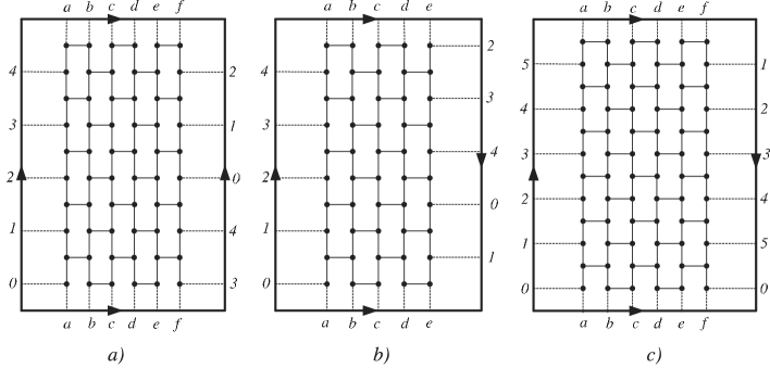
Figure 5: a) $H_{5,5,r}$ b) $H_{5,4,a}$ c) $H_{6,5,b}$

D) $H_{k,m,c}$ with $k$ even,   $k\geq 6$, $m\geq 1$. (Figure 6).

$$E(H_{k,m,c})=E(H)\cup\{\{z_{i},z_{i+k/2}\},\{z_{i},x_{i+k/2}\};\,0\leq i\leq(k/2)-1\}$$

An embedding of this graph in the Klein Bottle (Figure 6b) is obtained by deleting the edges $\{(2i,2j+1),(2i+1,2j+1)\}$ and $\{(2i+1,2j),(2i+2,2j)\}$ with $0\leq j\leq(k/2)-1$ and $0\leq i\leq m$ from a $(2m+2)\times k$ grid. Then, we add the edges $\{(0,2i+1),(2m+1,2i+1)|0\leq i\leq(k/2)-1\}$ to obtain two peripheral cycles, whose vertices of degree two are labeled $z_{i}=(i,0)$ and $x_{i}=(i,k-1)$ with $0\leq i\leq 2m+1$. Finally, we add the edges $\{\{z_{i},x_{2m+1-i}\}|0\leq i\leq 2m+1\}$.

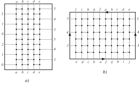
Figure 6: a) $H_{6,4,c}$ b) Embedding of $H_{6,4,c}$ in the Klein bottle

E) $H_{k,m,f}$ with $k$ odd, $m\geq 0$, $k\geq 7$ (Figure 7).

We add two cycles, $w_{0}w_{1}\ldots w_{k}w_{0}$ and $v_{0}v_{1}\ldots v_{k}v_{1}$, to a hexagonal cylinder of length $k$ and breadth $m$ as follows: $\{\{z_{i},w_{2i}\},\{x_{i},v_{2i}\}|0\leq i\leq(k-1)/2\}$. Then, a hexagonal tiling is obtained by adding edges between the vertices of degree two of this new structure. These edges are $\{\{z_{(k+2i+1)/2},w_{2i+1}\},\{x_{(k+2i+1)/2},v_{2i+1}\}|0\leq i\leq(k-1)/2\}$. An embedding of this graph in the Klein Bottle (Figure 7b), is obtained by deleting the same edges as in the previous case, from a $(2m+4)\times k$ grid. The edges $\{(0,2i+1),(2m+3,2i+1)|0\leq i\leq(k-1/2)-1\}$ are added giving rise to two peripheral cycles, whose vertices of degree two are labeled $z_{i}=(i,0)$ and $x_{i}=(i,k-1)$ with $0\leq i\leq 2m+3$. Finally, we add the edges $\{\{z_{0},x_{0}\},\{z_{i},x_{2m+4-i}\}|0\leq i\leq 2m+3\}$.

If $m=0$, we obtain the degenerate case called $H_{k,d}$ in [12].

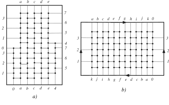
Figure 7: a) $H_{7,4,f}$ b) Embedding of $H_{7,4,f}$ in the Klein bottle

F) $H_{k,m,g}$ with $k\geq m+1$ and $m\geq 3$ (Figure 8a).

Let $TC_{k,m,2}$ be a twisted hexagonal cylinder of length $k$ and breadth $m$. In order to obtain a hexagonal tiling, we add the following edges:

$$E(H_{k,m,g})=E(TC_{k,m,2})\cup\{\{z_{i},w_{i}\},\{x_{i},v_{i}\};\,0\leq i\leq m\}$$

G) $H_{k,m,h}$ with $k\leq m-2$ and $k\geq 2$ (Figure 8b).

$$E(H_{k,m,h})=E(TC_{k,m,1})\cup\{\{z_{i},x_{i}\}|0\leq i\leq k\}\cup\{v_{i},w_{i}\};\,0\leq i\leq k-1\}$$

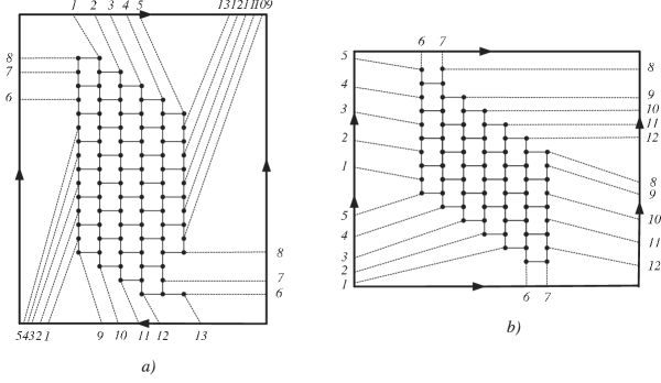
Figure 8: a) $H_{7,4,g}$ b) $H_{6,4,h}$

It is straightforward to verify that all the graphs we have defined are hexagonal tilings. We now prove that these families exhaust all the possible cases. In order to do so, we study the shortest essential cycles, the vertex transitivity and the chromatic number of all the hexagonal tilings defined. Every hexagonal tiling $G$ has an embedding in the torus or in the Klein bottle (if $G$ has $v$ vertices, $e$ edges and $h$ hexagons, then $v=2h$ and $2a=3v$ hence the Euler characteristic is zero).

Given two cycles $C$ and $C^{\prime}$ in a hexagonal tiling $G$, we say that $C$ is locally homotopic to $C^{\prime}$ if there exists a cell, $H$, with $C\cap H$ connected and $C^{\prime}$ is obtained from $C$ by replacing $C\cap H$ with $H-(C\cap H)$. A homotopy is a sequence of local homotopies. A cycle in $G$ is called essential if it is not homotopic to a cell. This definition is equivalent to the one given in a graph embedded in a surface [9]. Let $l_{G}$ be the minimum length of the essential cycles of $G$, $l_{G}$ is invariant under isomorphism.

Lemma 2.1.

Let $G$ be a hexagonal tiling of the types defined in A), B), C), D), E), F), G) then the length $l_{G}$ of their shortest essential cycles and the number of these cycles is:

$$G$$

$$G$$ number of essential cycles of length

Proof.

We have two different ways of pasting together $j$ ladders each one containing $i$ hexagons, from which we obtain two structures, called the ladder $i\times j$ and the displaced ladder $i\times j$ , shown in Figure 9.

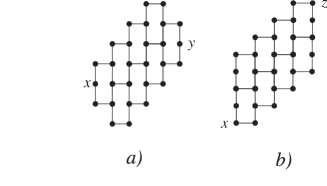
Figure 9: a) Displaced ladder $4\times 2$ b) Ladder $4\times 2$

For use below, note that the number of shortest paths between $x$ and $y$ or between $x$ and $z$ in a ladder $i\times j$ or in a displaced ladder $i\times j$ is $\left(\begin{array}[]{c}i+j\\ j\end{array}\right)$ and the length of these paths is $2(i+j)-1$.

Recall that every hexagonal tiling defined was obtained by adding edges to a hexagonal wall or to a hexagonal ladder (except for $H_{k,m,h}$, in which we also added two vertices). These edges are called exterior edges and every essential cycle must contain at least one of these edges (for $H_{k,m,h}$ the edges $\{(0,2k+m),(0,2k+m-1)\}$ and $\{(m-k-1,3k+2),(m-k-1,3k+1)\}$ are not considered exterior edges).

(1) $H_{k,m,r}$

If $k<m+1$, there is only one shortest path determined by each of the $(m+1)$ exterior edges of the form $\{(i,0),(i,2k-1)\}$, thus the resulting cycle has length $2k$.

If $r<\lfloor(m+1)/2\rfloor<\lfloor k/2\rfloor$, the $k$ edges of the form $\{z_{i},x_{i+r}\}$ give rise to the shortest essential cycles. The shortest paths joining the two ends of each one of these exterior edges have length $2m+1$ and each of them determine a displaced ladder $r+(m+1)/2\times(m-1)/2+1-r$ if $m$ odd or $(m+2)/2+r\times(m-2)/2+1-r$ if $m$ even; hence we have $k\left(\begin{array}[]{c}m+1\\ \lfloor(m+1)/2\rfloor-r\end{array}\right)$ shortest essential cycles of length $2m+2$.

If $\lfloor(m+1)/2\rfloor\leq r\leq\lfloor k/2\rfloor$ the shortest paths in the hexagonal wall that join the two ends of edges of the form $\{z_{i},x_{i+r}\}$ are composed of two parts. The first part is a path of length $2m+1$ crossing the hexagonal wall and the second part is a path of length $2r-2\lfloor(m+1)/2\rfloor$ along a peripheral cycle of the hexagonal cylinder. Each one of these exterior edges determine a displaced ladder $r-(m+1)/2\times m$ if $m$ odd or $r-(m+2)/2\times m$ if $m$ even.

(2) $H_{k,m,a}$

The $m+1$ edges of the form $\{(i,0),(i,2k-1)\}$ give rise to the same number of essential cycles as in the previous case.

If $k>m+1$, some exterior edges of the form $\{z_{0},x_{1}\},\{z_{1},x_{0}\},\{z_{i},x_{k+1-i}\}$ with $2\leq i\leq k-1$ determine shortest essential cycles of length $2m+2$. The shortest paths that join the two ends of these exterior edges generate displaced ladders $i\times j$ with $i=m+1-j$ and $0\leq j\leq m+1$. Hence, the number of shortest essential cycles is $\sum_{j=0}^{m+1}\left(\begin{array}[]{c}m+1\\ j\end{array}\right)=2^{m+1}$.

(3) $H_{k,m,b}$

If $k<m+1$ we have the same situation as in previous cases. If $k>m+1$, there are $m+1$ exterior edges of the form $\{z_{0},x_{0}\},\{z_{i},x_{k-i}\}$ with $1\leq i\leq k-1$ that determine shortest essential cycles of length $2m+2$. Two of these edges give rise to displaced ladders $(m+1)/2\times(m+1)/2$ and the rest of them, grouped four by four, give rise to displaced ladders $(m+1)/2+2j\times(m+1)/2-2j$, $0\leq j\leq(m-1)/4$.

(4) $H_{k,m,c}$

In order to count the shortest essential cycles, we use the embedding of this graph in the Klein bottle. If $4m+4<k+1$, each of the $k/2$ exterior edges of the form $\{(0,2i+1),(2m+1,2i+1)\}$ with $0\leq i\leq(k/2)-1$ determines a displaced ladder $(m+1)\times(m+1)$, in which the shortest paths that join the two ends of this exterior edge is $4m+3$. Hence, the number of shortest essential cycles is $(k/2)\left(\begin{array}[]{c}2m+2\\ m+1\end{array}\right)$ and the length of these cycles is $4m+4$.

If $4m+4>k+1$, there are just four exterior edges that give rise to shortest essential cycles of length $k+1$. The shortest paths that join the two ends of these edges generate ladders $(k/2)-1\times 1$, therefore the number of shortest essential cycles is $4\left(\begin{array}[]{c}(k/2)\\ 1\end{array}\right)=2k$.

(5) $H_{k,m,f}$

We also use the embedding of this graph in the Klein bottle. If $4m+8<k$ then reasoning as in the previous case, we obtain $(k-1)/2$ exterior edges that give rise to displaced ladders $(m+2)\times(m+2)$. If $4m+8>k$, we just have two shortest essential cycles of length $k$ generated by the edges $\{(2m+3,0),(2m+3,k-1)\}$ and $\{(m-1)/2,0),((m-1)/2,k-1)\}$.

(6) $H_{k,m,h}$

The exterior edge $\{x_{0},z_{0}\}$ determines one shortest essential cycle of length $2k+2$. The edges $\{(m-k-1,3k+2),(m,0)\}$, $\{(0,2k+m),(k+1,m-k-2)\}$ and $\{(j,2k+m-j),(k+j+1,m-k-j-2)\}$ with $1\leq j\leq m-k-2$ do not give rise to any shortest essential cycles. From the remaining, $2k+1$ edges we can determine different shortest essential cycles, but there are two exterior edges that generate the same shortest essential cycle. Every $k+1$ of these edges generate ladders $i\times j$ with $i=k-j$ and $0\leq j\leq k$ hence the number of shortest essential cycles is $2\sum_{j=0}^{k}\left(\begin{array}[]{c}k\\ j\end{array}\right)=2^{k+1}$.

(6) $H_{k,m,g}$

If $k=2m+1$ there are just two exterior edges, $\{z_{m},w_{m}\}$ and $\{x_{m},v_{m}\}$, that give rise to shortest essential cycles of length $2m+3$. If $k<2m+1$ and $k$ even, there are four exterior edges that determine shortest essential cycles of length $k+3$. These are the ones that cross the twisted hexagonal cylinder using $k/2$ hexagons. Each of these exterior edges generate a displaced ladder $1\times(k/2)$, therefore there are $4(k/2+1)$ shortest essential cycles. If $k>2m+1$ and $k$ odd, there are two exterior edges that allow to cross the twisted hexagonal cylinder using $(k+1)/2$ hexagons and each of these edges give rise to a displaced ladder $(k+1)/2\times 0$, hence there are two shortest essential cycles of length $k+2$. Finally, if $k>2m+1$ the length of the shortest essential cycles is the sum of the minimum length of two different paths. The first one, a path that crosses the hexagonal ladder and the second one, a path in a peripheral cycle of $TC_{k,m,2}$. In this last case we have not studied the number of shortest essential cycles. ∎

From Lemma 2.1, one can prove which of the hexagonal tilings defined are vertex-transitive graphs and which are not. A graph $G$ is vertex-transitive if for every two vertices of $G$, $u$ and $v$, there exits an isomorphism of graphs over $V(G)$, $\sigma$ such that $\sigma(u)=v$. This definition implies that all the vertices of $G$ have to belong to the same number of shortest essential cycles.

Lemma 2.2.

If $G$ is a hexagonal tiling of the type defined in A), B), C), D), E), F), G), then $G$ is vertex-transitive if $G$ is isomorphic to $H_{k,m,r}$ or $H_{4,m,a}$ with $m$ odd.

Lemma 2.3.

If $G$ is one of the hexagonal tilings defined in A), B), C), D), E), F), G), then the chromatic number of $G$ is given in the following table:

$$G$$

2 2 2 3 3 3 2

Proof.

Let $G$ be one of the hexagonal tilings defined in A), B), C), D), E), F), G). By Brooks’theorem we know that $\chi(G)<4$ and by Lemma 2.1 $H_{k,m,c}$, $H_{k,m,f}$ and $H_{k,m,g}$ have cycles of length odd therefore they can not be bipartite.

It is straightforward to prove that the chromatic number of a hexagonal cylinder $H$ of length $k$ and breadth $m$ is two for all $k$ and $m$. Due to the $2-$path condition, the vertices of degree two of the peripheral cycles have different colors. Hence, the chromatic number of $H_{k,m,r}$, $H_{k,m,a}$ and $H_{k,m,b}$ is two.

Since every hexagonal ladder admits a $2-$coloring then $TC_{k,m,1}$ is bipartite. We know that $H_{k,m,h}$ is obtained from $TC_{k,m,1}$ by adding edges between vertices of degree two of the same peripheral cycle. Now, each peripheral cycle of $TC_{k,m,1}$ has $2k+2$ vertices of degree two, $k+1$ of these can be assigned the same color and they are adjacent to the other $k+1$ vertices, which can be assigned the other color. Therefore the chromatic number of $H_{k,m,h}$ is two. ∎

Lemma 2.4.

The followings families of hexagonal tilings are not isomorphic:

A) $$H_{k,m,r}$$ with , and . If then and .

B) with , .

C) with even, odd, , .

D) with , even, .

E) with odd, , .

F) with , .

G) with , .

Proof.

By Lemmas 2.2 and 2.3 we just have to prove that the graphs given in each of the following cases can not be isomorphic.

(1) $H_{k,m,a}$ and $H_{k,m,b}$ are not isomorphic since every graph of the first family contains at most one parallel hexagonal Möbius circuit and every graph of the second family contains two.

(2) In order to prove that $H_{k,m,a}$ and $H_{k,m,h}$ are not isomorphic families, we are going to suppose that for every $k\geq 3$ and $m\geq 2$ there exits $k_{1}$ and $m_{1}$ such that $H_{k,m,a}$ and $H_{k_{1},m_{1},h}$ are isomorphic and thus obtain a contradiction. If both graphs are isomorphic, they have the same number of vertices, shortest essential cycles and the same length of these cycles, that is, $2k(m+1)=2(k_{1}+1)(m_{1}+1)$, $k_{1}=m$ and $k=m_{1}+1$. Hence, the minimum lengths of the non-oriented cycles of $H_{k,m,a}$ and $H_{k,m,h}$ are $2k$ and $4(m+1)$ respectively, and thus we reach a contradiction. With an analogous reasoning it follows that $H_{k,m,b}$ and $H_{k,m,h}$ are not isomorphic families.

(3) In general, the families $H_{k,m,c}$ and $H_{k,m,f}$ can not have the same number of vertices, and by Lemma 2.1 they cannot have the same number of shortest essential cycles or the same length of these cycles.

(4) By Lemma 2.1 it is clear that $H_{k,m,g}$ is not isomorphic neither to $H_{k,m,c}$ nor to $H_{k,m,f}$ because the length and the number of shortest essential cycles do not coincide in these graphs. ∎

Theorem 2.5.

If $G$ is a hexagonal tiling with $N$ vertices, then one and only one of the following holds:

A) $$G\simeq H_{k,m,r}$$ with , , , . If then

and .

B) with , , .

C) with , even, odd, , .

D) with , , even, .

E) with , odd, , .

F) with , , .

G) with , , .

Proof.

The argument of the proof is essentially the same as the one given in [12]. The difference between both proofs is that we include two new families to the list given in Theorem 3.1 of [12], $H_{k,m,g}$ and $H_{k,m,h}$. We consider the families $H_{k,d}$ and $H_{k,m,e}$ of [12] as degenerated cases of the families $H_{k,m,f}$ and $H_{k,m,r}$ respectively. Therefore we just study the case in which $G$ is a hexagonal tiling containing a hexagonal cylinder circuit of length $k$. We can extend this circuit either to a hexagonal cylinder of length $k$ and maximum breadth $m$, or to one of the two twisted hexagonal cylinders, $TC_{(k/2)-1,m,1}$ or $TC_{l,(k/2)-1,2}$. The first case is studied in [12] obtaining the families $H_{k,m,a}$, $H_{k,m,b}$, $H_{k,m,r}$, $H_{k,m,c}$ and $H_{k,m,f}$.

Assume that the hexagonal cylinder circuit is extended to a twisted hexagonal cylinder whose peripheral cycles, $C_{1}$ and $C_{2}$ are labeled as shown in Figure 3. If some vertex of $C_{1}$ is joined to some vertex of $C_{2}$, then by the $2-$path condition every vertex of degree two of $C_{1}$ has to be joined to a vertex of degree two of $C_{2}$. In a twisted hexagonal cylinder, we have that each two vertices of degree two of a peripheral cycle are at distance two except the couples $x_{0}z_{k}$, $w_{0}w_{1}$ and $v_{0}v_{1}$ in $TC_{k,m,1}$ and $z_{0}x_{k}$, $w_{k}v_{0}$ in $TC_{k,m,2}$. These couples determine the forms of joining vertices of degree two in order to obtain a hexagonal tiling. There are two possibilities, if $z_{i}$ is joined to $v_{i}$ and $x_{i}$ to $w_{i}$, we are in the case studied in [12] in which we extend the circuit to a hexagonal cylinder. If $z_{i}$ is joined to $w_{i}$ and $x_{i}$ to $v_{i}$, $G$ is isomorphic to $H_{l,(k/2)-1,g}$.

Assume now that no vertex of $C_{1}$ is adjacent to a vertex of $C_{2}$. Every vertex of degree two of each peripheral cycle has to be joined to another vertex of degree two of the same peripheral cycle. There is just one possibility, $z_{i}$ joined to $x_{i}$ and $v_{i}$ to $w_{i}$, thus $G$ is isomorphic to $H_{k/2-1,m,h}$. ∎

The geometric dual graph $G^{*}$ of a graph $G$ is a graph whose vertex set is formed by the faces of $G$ and two vertices are adjacent if the corresponding faces share an edge.

Theorem 2.6.

[12] Let $G^{\prime}$ be a connected $6$-regular graph and $C^{\prime}$ a collection of $3-$cycles in $G^{\prime}$ such that, for every vertex $v$ of $G^{\prime}$, there are precisely six cycles in $C^{\prime}$ that contain $v$ and their union is a $6-$wheel $W_{v}$ with $v$ as center. Suppose further that $G^{\prime}$ has no nonplanar subgraphs of radius 1. Then $G^{\prime}$ is a dual graph of a hexagonal tiling.

Theorems 2.5 and 2.6 give us a complete classification of locally $C_{6}$ graphs.

3 Relation with Locally Grid Graphs

In this section we establish a biyective minor relationship preserved by duality between hexagonal tilings with the same chromatic number and locally grid graphs. We want to remark that this minor relationship between hexagonal tilings, locally $C_{6}$ graphs and locally grid graphs is essential in the study of the Tutte uniqueness. The locally grid condition is different in that it involves not only a vertex and its neighbours, but also four vertices at distance two. Let $N(x)$ be the set of neighbours of a vertex $x$. We say that a $4-$regular, connected graph $G$ is a locally grid graph if for every vertex $x$ there exists an ordering $x_{1},x_{2},x_{3},x_{4}$ of $N(x)$ and four different vertices $y_{1},y_{2},y_{3},y_{4}$, such that, taking the indices modulo 4,

$$N(x_{i})\cap N(x_{i+1})$$

and there are no more adjacencies among $\{x,x_{1},\ldots,x_{4},y_{1},\ldots,y_{4}\}$ than those required by this condition (Figure 10).

Figure 10: Locally Grid Structure

A locally grid graph is simple, two-connected, triangle-free, and every vertex belongs to exactly four squares (cycles of length 4). A complete classification of locally grid graphs appears in [9]. They fall into several families and each of them has a natural embedding in the torus or in the Klein bottle.

Let $H=P_{p}\times P_{q}$ be the $p\times q$ grid, where $P_{l}$ is a path with $l$ vertices. Label the vertices of $H$ with the elements of the abelian group $\mathbb{Z}_{p}\times\mathbb{Z}_{q}$ in the natural way.

The Torus $T_{p,q}^{\delta}$ with $\,p\geq 5$, $\,0\leq\delta\leq p/2$, $\,\delta+q\geq 5\,$ if $\,q\geq 4$, $\,\delta+q\geq 6\,$ if $\,q=2,3\,$ or $\,4\leq\delta<p/2\,$ with $\,\delta\neq p/3,p/4\,$ if $\,q=1$.

$$E(T_{p,q}^{\delta})$$

The Klein Bottle $K_{p,q}^{1}$ with $\,p\geq 5$, $p$ odd, $\,q\geq 5$.

$$E(K_{p,q}^{1})$$

The Klein Bottle $K_{p,q}^{0}$ with $p\geq 5$, $p$ even, $q\geq 4$.

$$E(K_{p,q}^{0})$$

The Klein Bottle $K_{p,q}^{2}$ with $p\geq 5$, $p$ even, $q\geq 5$.

$$E(K_{p,q}^{2})$$

The graphs $S_{p,q}$ with $p\geq 3$ and $q\geq 6$.

If $p\leq q$ $E(S_{p,q})$ $=$ $E(H)$ $\cup$ $\{(j,0),(p-j,q-p+j)\},\,0\leq j\leq p-1\}$ $\cup$ $\{\{(0,i),(i,q-1)\},\,0\leq i\leq p-1\}$ $\cup$ $\{\{(0,i),(p-1,i-p)\},\,p\leq i\leq q-1\}$

If $q\leq p$ $E(S_{p,q})$ $=$ $E(H)$ $\cup$ $\{\{(j,0),(0,q-1-j)\},\,0\leq j\leq q-1\}$ $\cup$ $\{\{(p-1-i,q-1),(p-1,i)\},\,0\leq i\leq q-1\}$ $\cup$ $\{\{(i,q-1),(i+q,0)\},\,0\leq i\leq p-q-1\}$

Lemma 3.1.

If $G$ is a locally grid graph then $G^{*}=G$ if $G\in\{T_{p,q}^{r},K_{p,q}^{1},S_{p,q}\}$ and $(K_{p,q}^{0})^{*}=K_{p,q}^{2}$.

Proof.

Let $H$ be the $p\times q$ grid. $H$ has $(p-1)(q-1)$ squares (cycles of length four). If we replace every square by a vertex and two vertices are adjacent if the corresponding squares share an edge, then the resulting graph is a $(p-1)\times(q-1)$ grid. To construct locally grid graphs, we add edges between vertices of degree two and three of $H$. That is, we add $p+q-1$ squares. Now, if $G$ is a locally grid graph with $pq$ vertices, then $G^{*}$ has $pq$ vertices and it is obtained by adding edges between vertices of degree two and three of a $p\times q$ grid, denoted $H^{\prime}$. Vertices of $H$ and $H^{\prime}$ are labeled $(i,j)$ and $(i,j)^{*}$ respectively, for $0\leq i\leq p-1$ and $0\leq j\leq q-1$. Due to the classification theorem of locally grid graphs [9], we can consider the following cases.

(1) If $G\simeq T_{p,q}^{\delta}$, every vertex $(0,j)^{*}$ is associated to the square with vertices $(0,j-1)$, $(1,j-1)$, $(0,j+1)$ and $(1,j+1)$ then it has to be adjacent to the vertex of the square $(0,j-1)$, $(p-1,j-1)$, $(0,j+1)$, $(p-1,j+1)$, that is, $(p-1,j)^{*}$. Now, vertices $(i,0)^{*}$ and $(i+\delta,q-1)^{*}$ have to be adjacent since the squares $(i,0)$, $(i+1,0)$, $(i+\delta,q-1)$, $(i+\delta+1,q-1)$ and $(i+\delta,q-1)$, $(i+\delta+1,q-1)$, $(i+\delta,q-2)$, $(i+\delta+1,q-2)$ share an edge. Hence $V(G^{*})\simeq V(G)$ and $E(G^{*})\simeq E(G)$. (Figure 11a)

The cases in which $G\simeq K_{p,q}^{1}$ or $G\simeq S_{p,q}$ are similar to case (1) and we omit the proof for sake of brevity.

(2) If $G\simeq K_{p,q}^{0}$, reasoning as in (1) every vertex $(0,j)^{*}$ is adjacent to $(p-1,j)^{*}$. The vertices $(p-1,0)^{*}$ and $(p-1,q-1)^{*}$ have to be adjacent since the squares $(p-1,0)$, $(0,0)$, $(p-1,q-1)$, $(0,q-1)$ and $(p-1,q-1)$, $(p-1,q-2)$, $(0,q-2)$, $(0,q-1)$ share an edge. Since $p$ is even, $G^{*}$ is a locally grid graph and since it has two adjacencies, by [9] $G^{*}$ it is isomorphic to $K_{p,q}^{2}$. (Figure 11b) ∎

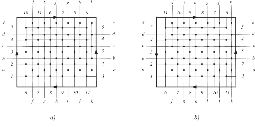
Figure 11: a) $T^{2}_{6,5}$ and its dual, $T^{2}_{6,5}$ (dotted) b) $K^{0}_{6,5}$ and its dual, $K^{2}_{6,5}$ (dotted)

Theorem 3.2.

Locally grid graphs are minors of hexagonal tilings (and by duality of locally $C_{6}$ graphs) by contraction of a perfect matching and deletion of the resulting parallel edges, except in one case in which a set of edges that do not form matching is contracted.

Proof.

Let $H$ be a hexagonal tiling, by Theorem 2.5 we know that $H$ belongs to one of the families $H_{k,m,r}$, $H_{k,m,a}$, $H_{k,m,b}$, $H_{k,m,c}$, $H_{k,m,f}$, $H_{k,m,g}$ and $H_{k,m,h}$. In order to prove that locally grid graphs are minors of hexagonal tilings, we are going to select a perfect matching in each one of the families, except in $H_{k,m,f}$ in which the selected edge set is not a matching. Then we obtain the locally grid graph by contracting the edges of this matching, and deleting parallel edges if necessary. There are just two cases in which we have to delete parallel edges, $H_{k,m,f}$ and $H_{k,m,h}$.

Let $C$ be a hexagonal cylinder of length $k$ and breadth $m$. We can take the following perfect matching, $P$, in $C$: $\{\{(i,2j),(i,2j+1)\}|0\leq i\leq m,0\leq j\leq k-1\}$. Then by contracting the edges in $P$ we obtain a $k\times(m+1)$ cylinder grid. This matching is also a perfect matching of $H_{k,m,r}$, $H_{k,m,a}$ and $H_{k,m,b}$ and no exterior edge of these graphs is contained in $P$. Therefore, we obtain by contracting $P$ in $H_{k,m,r}$ the graph $T_{k,m+1}^{r}$, in $H_{k,m,a}$ we obtain the graph $K_{k,m+1}^{0}$ if $k$ even and $K_{k,m+1}^{1}$ if $k$ odd, and in $H_{k,m,b}$ we obtain the graph $K_{k,m+1}^{2}$.

To select a perfect matching in $H_{k,m,c}$, we use the embedding of this graph in the Klein bottle and we take the same perfect matching that was specified in the previous case. By contracting the edges of $P$ we obtain the graph $K_{2m+2,k/2}^{0}$.

The case of $H_{k,m,f}$ is slightly different. We take the embedding of this graph in the Klein bottle, and consider the hexagons with vertices $(0,l)(0,l+1)(0,l+2)(1,l)(1,l+1)(1,l+2)$ where $l=2,\ldots,2k-5$. Then, $P$ is given by $P_{1}\cup P_{2}$, with:

$$P_{1}=\{\{(i,2j),(i,2j+1)\}|0\leq i\leq m,0\leq j\leq l/2\}$$

If the edges of $P$ are contracted and we delete the resulting parallel edges, we obtain $K_{2m+4,(k-1)/2}^{2}$.

For an illustration of these operations see the example given in Figure 13. In this example we start from $H_{7,4,f}$ and $P$ is given by the dotted edges. After contracting the selected edge set and deleting the resulting parallel edges we obtain $K^{2}_{12,3}$.

For a hexagonal ladder of length $k$ and breadth $m$, we take the following edges for the matching: $\{(0,m-1),(0,m)\}$, $\{(0,m+1),(0,m+2)\}$,$\ldots$ , $\{(0,2k+m-3),(0,2k+m-2)\}$, $\{(i,m-(i+1)),(i,m-i)\}$, $\{(i,m-(i+1)+2),(i,m-i+2)\}$, $\ldots$ , $\{(i,2k+m-(i+1))$,$(i,2k+m-i)\}$ with $1\leq i\leq m$. In order to obtain a perfect matching in $H_{k,m,h}$ we add the edges $\{(0,2k+m-1),(0,2k+m)\}$ and $\{(m-k-1,3k+2),(m,0)\}$. Then by contracting the edges of this matching and deleting the resulting parallel edge we obtain the locally grid graph $S_{m+1,k+1}$ with $k<m$. If we consider a similar selection of edges in a hexagonal ladder of length $k$ and breadth $m+1$ and we add $\{(0,2k+m),(m+1,2(k-m-1))\}$ we obtain a perfect matching of $H_{k,m,g}$ whose contraction gives the graph $S_{m+1,k+2}$ with $k\geq m+1$ (Figure 14).

For locally $C_{6}$ graphs, we follow the same procedure as for hexagonal tilings. In each case we take the set of dual edges associated to $P$ (Figure 12).

Figure 12: $c$ and $d$ are the dual edges of $a$ and $b$ respectively

If $G$ is the locally grid graph obtained from the contraction of the edges of $P$ and deletion of the resulting parallel edges in a hexagonal tiling $H$, then $G^{*}$ is obtained by the deletion of the set $P^{*}$ of dual edges associated to the perfect matching $P$ and contraction of the set of dual edges associated to the resulting parallel edges in a locally $C_{6}$ graph $H^{*}$. By Theorems 2.5 and 2.6 and Lemma 3.1, all the cases are determined. Figures 13 and 14 show two examples. In Figure 13, we start from $H_{7,4,f}^{*}$ selecting the dual edges of those belonging to the selected edge set of $H_{7,4,f}$. After applying the minor operations we obtain $K^{0}_{12,3}$, that is the dual graph of $K^{2}_{12,3}$. In Figure 14, we delete the dual edges of those belonging to the perfect matching of $H_{7,4,g}$ obtaining $S_{4,9}$.

To conclude:

Hexagonal

tiling

∎

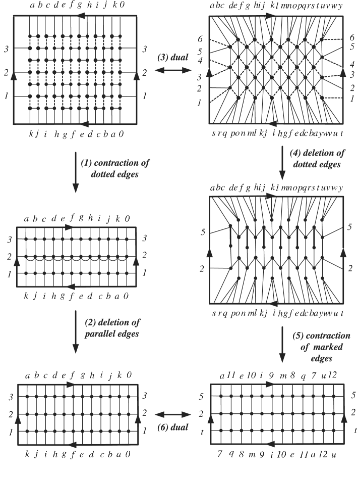
Figure 13: Deletion and contraction of the selected edge set in $H_{7,4,f}$ and $H_{7,4,f}^{*}$

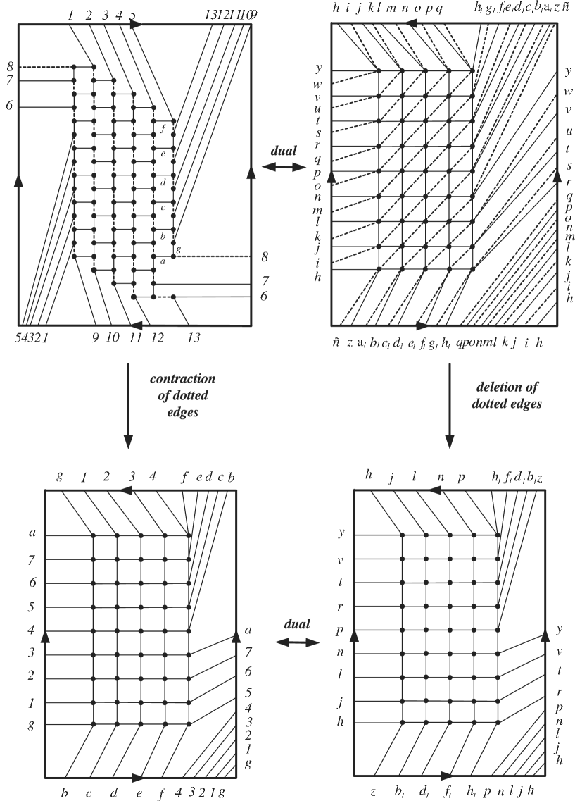
Figure 14: Deletion and contraction of the edges of a perfect matching in $H_{7,4,g}$ and $H_{7,4,g}^{*}$

References

- [1] A. Altshuler, Hamiltonian Circuits in some maps on the torus, Discret Math. 1(1972), 299-314.
- [2] A. Altshuler, Construction and enumeration of regular maps on the torus, Discret Math. 4(1973), 201-217.
- [3] T. Brylawski, J. Oxley, The Tutte polynomial and its applications, in: N. White (Ed.), Matroid Applications, Cambridge University Press, Cambridge, (1992).
- [4] S. Fisk, Geometric coloring theory, Advances in Math. 24(1977), 298-340.
- [5] S. Fisk, Variations on coloring, surfaces and higher dimensional manifolds , Advances in Math. 25(1977), 226-266.
- [6] D. Garijo, A. Márquez and M.P. Revuelta, Tutte Uniqueness of Locally Grid Graphs, Ars Combinatoria (to appear) (2005).
- [7] J.I. Hall, Locally petersen graphs, J. Graph Theory 4 (1980), 173-187.
- [8] F. Larrión, V. Neumann-Lara, Locally graphs are cycle divergent, Discr. Math. 215 (2000), 159-170.
- [9] A. Márquez, A. de Mier, M. Noy, M.P. Revuelta, Locally grid graphs:classification and Tutte uniqueness, Discr. Math. 266 (2003), 327-352.
- [10] S. Negami, Uniqueness and faithfulness of embedding of toroidal graphs, Discrete Math. 44(1983), no.2, 161-180.
- [11] S. Negami, Classification of 6-regular Klein bottle graphs, Res. Rep. Inf. Sci. T.I.T.A-96 (1984).
- [12] C. Thomassen, Tilings of the Torus and the Klein Bottle and vertex-transitive graphs on a fixed surface, Trans. Amer. Math. Soc. 323(1991), no.2, 605-635.