Local structure of random quadrangulations

Abstract

This paper is an adaptation of a method used in [10] to the model of random quadrangulations. We prove local weak convergence of uniform measures on quadrangulations and show that the local growth of quadrangulation is governed by certain critical time-reversed branching process and the rescaled profile converges to the reversed continuous-state branching process. As an intermediate result we derieve a biparametric generating function for certain class of quadrangulations with boundary.

1 Introduction

We consider the set of all finite rooted quadrangulations as a metric space with distance between two quadrangulation defined by

$$d(Q_{1},Q_{2})=\inf\Big{\{}\frac{1}{1+R}\Big{|}R:B_{R}(Q_{1})=B_{R}(Q_{2})\Big{\}},$$

where $B_{R}(Q)$ denotes the ball of radius $R$ around the root, and denote the completion of this space by ${\cal Q}$. Elements of ${\cal Q}$ other than finite quadrangulations are, by definition, infinite quadrangulations.

Theorem 1

The sequence $\mu_{N}$ of probability measures uniform on quadrangulations with $N$ faces converges weakly to a probability measure $\mu$ with support on infinite quadrangulations.

The measure $\mu$ defines certain random object – a uniform infinite quadrangulation, and we are interested in local properties of this object. We show that under distribution $\mu$ for each $R$ there exists a cycle $\gamma_{R}$, consisting of vertices at distance $R$ from the root and square diagonals between them, such that $\gamma_{R}$ separates the root from the infinite part of quadrangulation. Denote by $|\gamma_{R}|$ the length of such cycle.

Theorem 2

$|\gamma_{R}|$ is a Markov chain with transition probabilities given by

$$\mathop{\hbox{\sf P}}\nolimits\Big{\{}|\gamma_{r+n}|=k\Big{|}|\gamma_{r}|=l\Big{\}}=\frac{[t^{k}]F(t)}{[t^{l}]F(t)}\cdot\mathop{\hbox{\sf P}}\nolimits\{\xi_{n}=l|\xi_{0}=k\},$$

where $\xi$ is a critical branching process with offspring generating function

$$\varphi(t)=\frac{1}{2t}\Big{(}\sqrt{(t-9)(t-1)^{3}}-3+6t-t^{2}\Big{)},$$

and

$$F(t)=\frac{3}{4}\Big{(}\sqrt{\frac{9-t}{1-t}}-3\Big{)}$$

is the generating function of it’s stationary measure.

Corollary 1

The random variable $2|\gamma_{R}|/R^{2}$ converges in distribution to the $\Gamma(3/2)$ law.

Knowing that the properly rescaled branching processes converge to continuous-time branching processes, it is natural to look for the continuous-time limit of the rescaled profile $|\gamma_{tR}|/R^{2}$. An exact statement is provided by Theorem 4 in Section 4.

Finally, we propose the following conjecture.

Conjecture 1

Let $\ell(R)$ be the cycle of minimal length in a uniform infinite quadrangulation $Q$ that separates the ball $B_{R}(Q)$ from the infinite part of quadrangulation. Then it’s length $|\ell(R)|$ is linear in $R$ as $R\to\infty$

In 3.5 we show how the upper bound follows from the branching construction used in proof of Theorem 2. The lower bound remains an open question.

2 Some facts on quadrangulations

2.1 Definitions

Consider a finite planar graph embedded into the sphere, such that each component of the complement to the graph is homeomorphic to a disk. A planar map is an equivalence class of such embedded graphs with respect to orientation-preserving homeomorphisms of the sphere.

A planar map is rooted if a directed edge, called the root, is specified. A rooted planar map has no nontrivial automorphisms. We will refer to the tail vertex of the root as root vertex, and to distance from any vertex of a map to this vertex as distance to the root.

Quadrangulation is a rooted planar map such that all it’s faces are squares, i.e. it’s dual graph is four-valent. Note that every quadrangulation is bipartite (this follows from the fact that any subset of faces in a quadrangulation is necessarily bounded by an even number of edges).

In the following we will distinguish two type of faces based on the distances from the vertices around the face to the root: these distances are either $(R-1,R,R+1,R)$ or $(R-1,R,R-1,R)$ for some $R$. Since every quadrangulation is bipartite, there are no $(R,R)$ edges.

Quadrangulation with a boundary is rather self-evident notion; formally this is a planar map with all faces being squares except one distinguished face which can be an arbitrary even-sided polygon. When drawing the quadrangulation it is convenient to represent this distinguished face by the infinite face. This face is then excluded from ”faces” of quadrangulation and is referred to as ”boundary”.

We say that a quadrangulation has simple boundary, if all vertices of the boundary are distinct (i.e. no vertex is met twice when walking around the boundary), and every second vertex has degree two (see fig. 1).

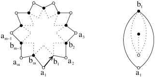
Figure 1: Typical quadrangulation with simple boundary and an example with minimal boundary length.

2.2 Some enumeration results

Let $C(N)$ be the number of rooted quadrangulations with $N$ faces, and let $C(N,m)$ be the number of rooted quadrangulations with $N$ faces and with simple boundary of length $2m$, such that the root is located on the boundary and root vertex has degree two.

We will need the following enumeration results (see section 5 for details)

$$q(x)=\sum_{N=0}^{\infty}C(N)x^{N}=\frac{4}{3}\frac{2\sqrt{1-12x}+1}{(\sqrt{1-12x}+1)^{2}},$$ (1)

$$U(x,y) = \sum_{N,m}C(N,m)x^{N}y^{m}$$ (2)

$$= \frac{1}{2}\Big{(}y-xy^{2}-1+\sqrt{y^{2}-2xy^{3}-2y+4xyq(x)+(xy^{2}-1)^{2}}\Big{)}$$

The function $U(x,y)$ is analytic around $(0,0)$ and it’s first singularity in $x$ for small $y$ coincides with the singularity of $q(x)$, i.e. $x_{0}=1/12$. From the expansion near this point

$$U(x,y)\Big{|}_{x=x_{0}-t}=A(y)+A_{1}(y)t+B(y)t^{3/2}+O(t^{2}),$$ (3)

where

$$A(y)=\frac{1}{24}\sqrt{(y-18)(y-2)^{3}}-\frac{1}{2}+\frac{y}{2}-\frac{y^{2}}{24},$$

$$A_{1}(y)=\frac{y^{2}}{2}+\frac{y}{2}\frac{y^{2}-10y-32}{\sqrt{(18-y)(2-y)}},\qquad B(y)=\frac{64\sqrt{3}\cdot y}{\sqrt{(y-18)(y-2)^{3}}},$$

one finds the asymptotic of $C(N,m)$ as $N\to\infty$:

$$C(N,m)=\frac{b(m)}{\Gamma(\frac{3}{2})}N^{-5/2}x_{0}^{-N}\Big{(}1+O(N^{-1/2})\Big{)},\qquad b(m)=[y^{m}]B(y).$$ (4)

Note also that $[y]U(x,y)=xq(x)$, thus

$$C(N)=C(N+1,1)=\frac{b(1)}{x_{0}\Gamma(\frac{3}{2})}N^{-5/2}x_{0}^{-N}\Big{(}1+O(N^{-1/2})\Big{)}.$$ (5)

2.3 Basic probabilities

First let us specify more exactly the definition of ball $B_{R}(Q)$. Given a rooted quadrangulation $Q$, $B_{R}(Q)$ consists of all faces that have at least one vertex at distance strictly less than $R$ from the root. With this definition there are only faces of type $(R-1,R,R+1,R)$ at the boundary of $B_{R}(Q)$.

Say we want to compute the probability for a uniformly distributed $N$-faced quadrangulation $S_{N}$ to have a particular root neighbourhood $K$. Suppose that $K$ has $n$ faces and, for simplicity, a connected boundary of length $2m$, so that $K$ is a quadrangulation with simple boundary. Take any other quadrangulation $S$ with simple boundary of the same length. We can glue $K$ and $S$ as follows:

• cut $m$ half-squares around the boundary of $K$, so that the resulting map $K^{\prime}$ is bounded by $m$ diagonals;

• repeat the same for $S$, obtaining a map $S^{\prime}$ bounded by $m$ diagonals;

• identify the boundaries of $K^{\prime}$ and $S^{\prime}$ (see fig. 2).

The resulting map $(K^{\prime}+S^{\prime})$ has $m$ faces less than $K$ and $S$ had together, i.e. if $S$ has $N-n+m$ faces, $(K^{\prime}+S^{\prime})$ would have $N$ faces.

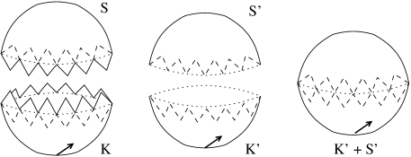
Figure 2: Glueing two quadrangulations with simple boundary.

It’s easy to see that the process on fig. 2 is reversible. Indeed, take a quadrangulation $Q$ with root neighbourhood $K$, cut it in two along the boundary of $K^{\prime}$, and add $m$ half-squares to each part. This will give $K$ and some quadrangulation with simple boundary, which then can be used to reconstruct $Q$.

Thus for each of $C(N-n+m,m)$ maps $S$ with $N-n+m$ faces we get a different $N$-faced quadrangulation, and every $N$-faced quadrangulation with root neighbourhood $K$ is obtained this way. In other words

$$\mathop{\hbox{\sf P}}\nolimits\{B_{R}(S_{N})=K\}=\frac{C(N-n+m,m)}{C(N)}.$$

Combining this with asymptotics (4), (5) we get

Lemma 2.1

Given a quadrangulation $K$ with $n$ faces and simple boundary of length $2m$, such that $B_{R}(Q)=K$ for some $Q$,

$$\lim_{N\to\infty}\mathop{\hbox{\sf P}}\nolimits\{B_{R}(S_{N})=K\}=\frac{b(m)}{b(1)}x_{0}^{n-m+1},$$ (6)

where $S_{N}$ denotes uniformly distributed random quadrangulation with $N$ faces.

Figure 3: Quadrangulation $Q$, ball $B_{R}(Q)$ and hull ${\hat{B}}_{R}(Q)$.

In general case, however, the boundary of $B_{R}(Q)$ may have multiple disjoint components (fig. 3, middle). Following the same reasoning as above and assuming that $K$ has $k$ boundary components (”holes”) of length $2m_{1},\ldots,2m_{k}$ and $n$ faces, we’ll get the following formula

$$\mathop{\hbox{\sf P}}\nolimits\{K=B_{R}(S_{N})\}=\frac{1}{C(N)}\sum_{N_{1}+\ldots+N_{k}=N-n}\,\,\prod_{j=1}^{k}C(N_{j}+m_{j},m_{j}).$$ (7)

Here we count all possible ways to ”fill” the $k$ holes in $K$ using quadrangulations with appropriate boundary length; $N_{j}$ is the number of internal faces in quadrangulation used to fill $j$th hole.

Due to the factor $N^{-5/2}$ in asymptotics (4), for large $N$ the only significant terms in sum (7) are those where one of $N_{j}$ has order $N$, while all others are finite. This means that in a large random quadrangulation $S_{N}$ conditioned to $B_{R}(S_{N})=K$, with high probability only one of the ”holes” in $K$ contains the major part of the quadrangulation (we could calculate exact probabilities here, but this is not necessary).

Such observation motivates the following definition: given quadrangulation $Q$, take the ball $B_{R}(Q)$ and glue all but the largest components of the complement $Q\backslash B_{R}(Q)$ back to the ball. The resulting map is called the $R$-hull of quadrangulation $Q$, and is denoted by ${\hat{B}}_{R}(Q)$.

Unlike the boundary of the ball, the boundary of ${\hat{B}}_{R}(Q)$ is always connected (see fig. 3, right), but similarly to $B_{R}(Q)$ there there are only faces of type $(R,R+1,R,R-1)$ at the boundary of ${\hat{B}}_{R}(Q)$, thus the hull is a quadrangulation with simple boundary.

Limiting probabilities for the hull and exactly the same as for the ball:

Lemma 2.2

Given a quadrangulation $K$ with $n$ faces and boundary of length $2m$, such that ${\hat{B}}_{R}(Q)=K$ for some $Q$,

$$\lim_{N\to\infty}\mathop{\hbox{\sf P}}\nolimits\{{\hat{B}}_{R}(S_{N})=K\}=\frac{b(m)}{b(1)}x_{0}^{n-m+1}$$ (8)

where $S_{N}$ denotes uniformly distributed random quadrangulation with $N$ faces.

Proof. The proof is essentially the same as for the ball with single hole. Given $K$, every quadrangulation $(K^{\prime}+S^{\prime})$, obtained by glueing $K$ and any quadrangulation $S$ with simple boundary of length $2m$, has the same $R$-hull ${\hat{B}}_{R}(K^{\prime}+S^{\prime})=K$ as soon as the number of faces in $S$ is large enough (say larger than $n$). Thus for $N>2n$

$$\mathop{\hbox{\sf P}}\nolimits\{{\hat{B}}_{R}(S_{N})=K\}=\frac{C(N-n-m,m)}{C(N)}$$

and the limit (8) follows.

2.4 A note on convergence of measures

The limiting probabilities (8) define a measure $\mu$ on ${\cal Q}$, such that for all $K$ and $R$

$$\mu_{N}(Q:\,B_{R}(Q)=K)\to\mu(Q:\,B_{R}(Q)=K)\quad\mbox{as $N\to\infty$}.$$

However, since ${\cal Q}$ is not compact, the existence of this limit does not, by itself, imply weak convergence of $\mu_{N}$ to $\mu$. For the weak convergence to follow one has to show that $\mu$ is indeed a probability measure. See [2, section 1.2] for detailed discussion of this question.

In the next section we will evaluate the sum of limiting probabilities (8) over all possible $R$-hulls $K$ and show that for each $R$ this sum equals one. This will prove Theorem 1.

3 Quadrangulation and branching process

3.1 Hull decomposition

Consider $K$ such that $K={\hat{B}}_{R}(Q)$ for some quadrangulation $Q$. If $Q$ is large enough (e.g. if the number of faces in $Q$ is at least twice that of $K$) then

$${\hat{B}}_{R}(Q)\supseteq{\hat{B}}_{R-1}(Q)\supseteq\ldots\supseteq{\hat{B}}_{1}(Q),$$

and this sequence doesn’t actually depend on $Q$.

As noticed earlier, the hull has simple boundary. Let us denote the vertices of the boundary of ${\hat{B}}_{R}(Q)$ by $(a_{1},b_{1},\ldots,a_{m},b_{m})$, as on fig. 1, starting from some arbitrarily chosen vertex and so that all $a_{i}$’s are situated at distance $R+1$ from the root, and all $b_{i}$’s at distance $R$ from the root.

Let $\gamma_{R}$ be the cycle consisting of vertices $b_{1},\ldots,b_{m}$ and square diagonals between them. Define cycles $\gamma_{R-1},\ldots,\gamma_{1}$ similarly. A layer $L_{R}$ is a part of quadrangulation contained between cycles $\gamma_{R-1}$ and $\gamma_{R}$. It turns out that the layer has very simple structure:

• each edge $(b_{i-1},b_{i})$ of it’s upper boundary $\gamma_{R}$ is a diagonal in a square that touches it’s lower boundary $\gamma_{R-1}$ at some point $c_{i}$;

• points $c_{i}$ are cyclically ordered around $\gamma_{R-1}$ and there are $l_{i}\geq 0$ edges of $\gamma_{R-1}$ between $c_{i}$ and $c_{i+1}$ ($l_{i}=0$ if $c_{i}$ and $c_{i+1}$ both refer to the same vertex).

Let us call the area $(c_{i},b_{i},b_{i+1},c_{i+1})$ a block. A layer is uniquely (up to rotation related to choice of vertex $a_{1}$) characterized by a sequence of blocks.

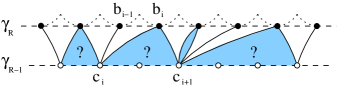
Figure 4: Layer structure. Contents of filled areas is unknown.

The internal structure of a block is not as simple – it can contain arbitrary large subquadrangulation, which can have vertices at distance more than $R$ from the root. This is here where the ”reattached” components of ${\hat{B}}_{R}(Q)\backslash B_{R}(Q)$ go. Note that even with $l_{i}=0$ the block contents can be non-trivial (fig. 5, right).

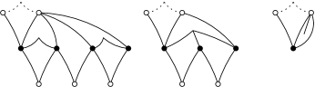
Figure 5: Possible internal structure of a block.

Fortunately there is a bijection between blocks and a class of quadrangulations with simple boundary counted by $C(N,m)$ in section 2.2. The block is converted to quadrangulation via the procedure illustrated on fig. 6. Clearly, this procedure is reversible: one has to choose the topmost vertex on the right-hand side of fig. 6 as the root vertex of the quadrangulation; then the block is recovered by cutting the quadrangulation along the edge, opposite to the root in the rooted square.

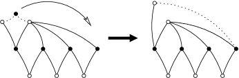
Figure 6: Converting a block to a quadrangulation with simple boundary.

To conclude: the $R$-hull consists of $R$ layers, each layer consists of one or more blocks, and each block is essentially a quadrangulation with simple boundary.

3.2 Tree structure

The layer/block representation suggests the following tree structure: let the edges of $\gamma_{r}$, $r=1,\ldots,R$ be the nodes of a tree, and connect each edge of $\gamma_{r}$ to the edges of $\gamma_{r-1}$ that belong to the same block.

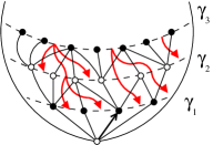
Figure 7: Fragment of tree structure on quadrangulation.

The whole hull $K$ then can be represented by a planar forest $T_{K}$ of height $R$, where with each vertex one associates a quadrangulation with simple boundary, so that for a vertex $v_{i}$ of outdegree $l_{i}$ the associated quadrangulation has boundary length $2(l_{i}+1)$. Unfortunately this representation is not unique: given $T_{K}$ and it’s associated quadrangulations, we can reconstruct $K$ and the root vertex of $K$, but not the root edge. In order to include the information on root edge position into the tree structure, we apply to $K$ the following modification (see fig. 8):

• cut $K$ along the root edge, obtaining a hole of length two;

• attach a new square to the boundary of this hole;

• identify two remaining edges of this square and make the resulting edge a new root.

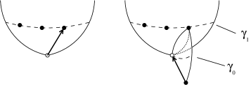
Figure 8: Adding an extra square at the root.

One diagonal of a new square has it’s ends identified; this gives an extra cycle $\gamma_{0}$, which always has length one. In terms of tree structure this means that we add one child to some $\gamma_{1}$-vertex of $T_{K}$; this new vertex has no associated quadrangulation. Call this extended forest a skeleton of hull $K$.

Note that since there is no natural ”first” edge in $\gamma_{R}$, the tree structure implies only cyclic order on the trees of $T_{K}$. However for convenience we will consider $T_{K}$ as linearly ordered, and will keep in mind that the same tree structure can be represented by several forests, which differ by cyclic permutation of trees.

Apart from this ambiguity the hull $K$ is uniquely characterized by it’s skeleton and associated quadrangulations.

3.3 Analogy with branching process

Branching process is a random process with discrete time. It starts with one or more particles, and at each step every particle independently of the others is replaced by zero, one, or more child particles according to the offspring distribution $\{p_{i}\}_{i=0}^{\infty}$, which remains fixed throughout the whole process.

It is convenient to represent the trajectory of a branching process by a planar tree (or forest, if starting from multiple particles). The probability to see certain trajectory tree $T$ is then a product over all vertices of probability for a particle to have an offspring of size equal to the outdegree of the vertex:

$$\mathop{\hbox{\sf P}}\nolimits\{T\}=\prod_{v\in T}\left.p_{i}\right|_{i={\rm outdeg}(v)}$$ (9)

We will attempt to do the reverse: apply the theory of branching processes to the analysis of the tree structure described above.

Say we want to compute the probability for an $R$-hull of uniformly distributed quadrangulation $S_{N}$ to have a particular skeleton $T_{K}$. As explained above, every such $R$-hull is obtained from $T_{K}$ by choosing an appropriate set of associated quadrangulations. On the other hand, taking for every vertex $v_{i}\in T_{K}$ with outdegree $l_{i}$ a quadrangulation with simple boundary of length $2(l_{i}+1)$ will give a valid $R$-hull, which has the required skeleton. A simple calculation shows that if $i$’th associated quadrangulation has $n_{i}$ faces, the hull will have $m-1+\sum_{i}(n_{i}-1)$ faces, where $m$ is half the length of hull boundary (or equivalently the number of trees in the skeleton).

Combining this with Lemma 2.2, we’ll get the following formula

$$\lim_{N\to\infty}\hbox to0.0pt{$\displaystyle\mathop{\hbox{\sf P}}\nolimits\{skel_{R}(S_{N})=T_{K}\}$\hss}$$ (10)

$$= \sum_{n_{1},n_{2},\ldots=0}^{\infty}\Big{(}\prod_{v_{i}\in T_{K}}C(n_{i},l_{i}+1)\Big{)}\frac{b(m)}{b(1)}x_{0}^{\Sigma_{i}(n_{i}-1)}$$

$$= \frac{b(m)}{b(1)}\prod_{v_{i}\in T_{K}}\sum_{n_{i}=0}^{\infty}C(n_{i},l_{i}+1)x_{0}^{n_{i}-1}$$

$$= \frac{b(m)}{b(1)}\prod_{v_{i}\in T_{K}}\frac{1}{x_{0}}[y^{l_{i}+1}]A(y),$$

where $A(y)$ is the first coefficient of expansion (3).

The last product in (10) looks similar to the product (9). There is however one important difference – product terms of (10) do not define a probability distribution.

In order to make the analogy with branching process complete, we apply the following normalization procedure: for each square crossed by one of the cycles $\gamma_{0},\ldots,\gamma_{R}$ write $y_{0}$ on the upper half-square and $y_{0}^{-1}$ on the lower half-square. Each block then gets an extra term $y_{0}^{l_{i}-1}$; plus there is $y_{0}^{m}$ on the upper boundary of the hull, due to $m$ half-squares above $\gamma_{R}$, and $y_{0}^{-1}$ due to one half-square below $\gamma_{0}$. So we can continue (10) with

$$\ldots = \frac{b(m)}{b(1)}y_{0}^{m-1}\prod_{v_{i}\in T_{K}}\frac{1}{x_{0}}y_{0}^{l_{i}-1}[y^{l_{i}+1}]A(y)$$ (11)

$$= \frac{b(m)}{b(1)}y_{0}^{m-1}\prod_{v_{i}\in T_{K}}[t^{l}_{i}]\varphi(t),$$

where

$$\varphi(t)=\frac{1}{tx_{0}y_{0}^{2}}A(y_{0}t).$$

For the Taylor coefficients of $\varphi(t)$ to define a probability distribution it has to satisfy the equation $\varphi(1)=1$, which is equivalent to $A(y_{0})=x_{0}y_{0}$. Solving this last equation we find $y_{0}=2$ and

$$\varphi(t)=\frac{1}{2t}\Big{(}\sqrt{(t-9)(t-1)^{3}}-3+6t-t^{2}\Big{)}.$$

3.4 Remaining proofs

Proof of Theorem 1.  Using (10), (11) let us compute the probability $|\gamma_{R}|=m$ with respect to $\mu$.

$$\mathop{\hbox{\sf P}}\nolimits_{\mu}\{|\gamma_{R}|=m\}=\frac{1}{m}\frac{b(m)}{b(1)}y_{0}^{m-1}\sum_{T}\prod_{v_{i}\in T}[t^{l}_{i}]\varphi(t),$$ (12)

where the sum is taken over all forests $T$ of height $R+1$ that have $m$ vertices on level $R$ and exactly one vertex at level $0$ (in ”reversed” notation). The term $1/m$ appears in (12) because for each $R$-hull with $|\gamma_{R}|=m$ there are exactly $m$ linearly ordered forests describing the tree structure of this hull.

Let $\xi$ be a branching process with offspring generating function $\varphi(t)$. The sum in (12) can be interpreted as the probability for $\xi$ starting from state $m$ at time $0$, to reach state $1$ at time $R$. Let

$$F(t)=\sum_{m=0}^{\infty}\frac{b(m)/m}{b(1)}y_{0}^{m-1}t^{m}.$$

Then (12) can be rewritten as

$$\mathop{\hbox{\sf P}}\nolimits_{\mu}\{|\gamma_{R}|=m\}=[t^{m}]F(t)\cdot\mathop{\hbox{\sf P}}\nolimits\{\xi_{R+1}=1|\xi_{0}=m\}.$$ (13)

The $R$-step transition probabilities of a branching process are expressed via it’s offspring generating function as

$$\mathop{\hbox{\sf P}}\nolimits\{\xi_{R}=n|\xi_{0}=m\}=[t^{n}]\varphi_{R}^{m}(t),$$

where $\varphi_{R}(t)$ stands for the $R$’th iteration of $\varphi(t)$. Thus

$$\sum_{m=1}^{\infty}\mathop{\hbox{\sf P}}\nolimits_{\mu}\{|\gamma_{R}|=m\}=[t]F(\varphi_{R}(t)).$$

Since $b(m)=[y]B(y)$, where $B(y)$ is a coefficient in (3), we find that

$$F(t)=\frac{1}{y_{0}b(1)}\int\limits_{0}^{ty_{0}}\frac{B(y)}{y}\,dy=\frac{3}{4}\Big{(}\sqrt{\frac{9-t}{1-t}}-3\Big{)}$$

and a direct computation shows that $F(t)$ satisfies the Abel equation

$$F(\varphi(t))-F(\varphi(0))=F(t).$$ (14)

In particular this means that $[t]F(\varphi_{r}(t))=[t]F(t)$ for all $r$, and since $[t]F(t)=1$

$$\sum_{m=1}^{\infty}\mathop{\hbox{\sf P}}\nolimits_{\mu}\{|\gamma_{R}|=m\}=1.$$

But the last sum is also the sum of limiting probabilities (8) over all possible $R$-hulls. This completes the proof of Theorem 1.

Proof of Theorem 2.  To prove theorem 2 first note that

$$\mathop{\hbox{\sf P}}\nolimits_{\mu}\{|\gamma_{r}|=l,|\gamma_{r+n}|=k\}=[t^{k}]F(t)\cdot\mathop{\hbox{\sf P}}\nolimits\{\xi_{n}=l,\xi_{r+n}=1|\xi_{0}=k\}.$$

This formula is obtained by taking sum of probabilities (11) over all skeletons with $k$ vertices at level $(r+n)$ and $l$ vertices at level $r$. Now since $\xi$ is Markovian

$$\mathop{\hbox{\sf P}}\nolimits\{\xi_{n}=l,\xi_{r+n}=1|\xi_{0}=k\}=\mathop{\hbox{\sf P}}\nolimits\{\xi_{n}=l|\xi_{0}=k\}\mathop{\hbox{\sf P}}\nolimits\{\xi_{r+n}=1|\xi_{n}=l\},$$

and combining this with (13) we get

$$\mathop{\hbox{\sf P}}\nolimits\Big{\{}|\gamma_{r+n}|=k\Big{|}|\gamma_{r}|=l\Big{\}}=\frac{[t^{k}]F(t)}{[t^{l}]F(t)}\cdot\mathop{\hbox{\sf P}}\nolimits\{\xi_{n}=l|\xi_{0}=k\}.$$ (15)

The Abel equation (14) means that $F(t)$ is a generating function of stationary measure for process $\xi$ (see [8], section 1.4), so the right-hand side of (15) is indeed the transition probability for a reversed branching process.

Proof of Corollary 1.  The $R$th iteration of $\varphi(t)$ is

$$\varphi_{R}(t)=1-\frac{8}{\Big{(}\sqrt{\frac{9-t}{1-t}}+2R\Big{)}^{2}-1},$$ (16)

this can be verified by induction. The distribution of $|\gamma_{R}|$ is given by

$$\mathop{\hbox{\sf P}}\nolimits\{|\gamma_{R}|=m\}=[t^{m}]F(t)\cdot[t]\varphi_{R}^{m}(t).$$

Calculating explicitly

$$[t]\varphi_{R}^{m}(t)=\frac{4}{3}m(2R+3)\frac{(R^{2}+3R)^{m-1}}{(R^{2}+3R+2)^{m+1}},$$

$$[t^{m}]F(t)=\frac{3}{\sqrt{2\pi}}m^{-1/2}+O(1),$$

and putting $m=xR^{2}$ we find for large $R$

$$\mathop{\hbox{\sf P}}\nolimits\{|\gamma_{R}|=xR^{2}\}=\frac{8}{\sqrt{2\pi}}\frac{x^{1/2}e^{-2x}}{R^{2}}+O(\frac{1}{R^{3}}).$$

This implies convergence of $2|\gamma_{R}|/R^{2}$ to $\Gamma(3/2)$ law.

3.5 Linear cycle

The cycle $\gamma_{R}$ is a natural analog of circle in Euclidean geometry: this is a closed curve, and it’s points are situated exactly at distance $R$ from the center (root). The relation $|\gamma_{R}|=O(R^{2})$ is, however, quite different from the usual $L=2\pi R$.

A natural question to ask is what happens, if we weaken restrictions, for example, by allowing the separating cycle to contain any points at distance at least $R$ from the root?

It turns out that there exists such cycle with length linear in $R$. This cycle is built as follows:

• consider all vertices of $\gamma_{R}$, and group together the vertices that have common ancestor in $\gamma_{2R}$;

• in each group there is a leftmost element and a rightmost element. Take a path from the leftmost up to the common ancestor, then down to the rightmost (such path has approximately $2R$ steps);

• join these paths together to form a separating cycle $\ell_{R}$. $\gamma_{2R}$ that have non-empty offspring at $\gamma_{R}$.

The length of $\ell_{R}$ is $2R\cdot\theta_{R}$, where $\theta_{R}$ is the number of vertices at $\gamma_{R2}$ that have nonempty offspring at $\gamma_{R}$. It remains to show that $\theta_{R}$ has finite distribution.

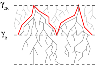
Figure 9: fragment of linear cycle

From (15) we have

$$\mathop{\hbox{\sf P}}\nolimits\{\theta_{R}=k|\gamma_{R}=m\}=\sum_{n=1}^{\infty}\frac{[t^{n}]F(t)}{[t^{m}]F(t)}{n\choose k}\varphi_{R}^{n-k}(0)\cdot[t^{m}](\varphi_{R}(t)-\varphi_{R}(0))^{k},$$

$$\mathop{\hbox{\sf P}}\nolimits\{\gamma_{R}=m\}=[t^{m}]F(t)\cdot[t]\varphi_{R}^{m}(t),$$

thus

$$\mathop{\hbox{\sf E}}\nolimits(y^{\theta_{R}}|\gamma_{R}=m)=\frac{[t^{m}]F\Big{(}\varphi_{R}(0)+y(\varphi_{R}(t)-\varphi_{R}(0))\Big{)}}{[t^{m}]F(t)},$$

$$\mathop{\hbox{\sf E}}\nolimits y^{\theta_{R}}=[t]F\Big{(}\varphi_{R}(0)+y(\varphi_{2R}(t)-\varphi_{R}(0))\Big{)}.$$

The last expression being a generating function of $\theta_{R}$, a direct calculation of it’s derivatives at $y=1$ shows that as $R\to\infty$ the first and second moments of $\theta_{R}$ converge to $11/2$ and $171/2$ respectively. This provides an upper bound for Conjecture 1.

4 Convergence to continuous process

4.1 Identifying the limit

Given the results of previous section, it is natural to expect the convergence of rescaled process

$$\frac{|\gamma_{tR}|}{R^{2}},\qquad t\in[0,1]$$ (17)

as $R\to\infty$ in sence of weak convergence in $D[0,1]$ (the space of functions without discontinues of second kind [5]). We will start from identifying the limit $\zeta_{t}$ of the rescaled branching process

$$\frac{\xi_{tR}}{R^{2}},\qquad t\in[0,1].$$ (18)

As shown by Lamperti [11], any possible limit of a sequence of rescaled branching processes is a countinous-state branching process, i.e. a Markov process on $[0,\infty)$ with right-continuous paths, whose transition probabilities satisfy the branching property

$$P_{t}(x+y,\cdot)=P_{t}(x,\cdot)*P_{t}(y,\cdot)$$

for all $t,x,y\geq 0$. Every continuous-state branching process is fully characterized by it’s Laplace transform

$$\int_{0}^{\infty}e^{-\lambda y}P_{t}(x,dy)=\exp(-xu_{t}(\lambda)),\quad\lambda\geq 0,$$

and in particular by the function $u_{t}$. To derieve the function corresponding to $\zeta_{t}$ we use a theorem due to Zolotarev ([17], Theorem 7),

Theorem 3 (Zolotarev)

Let $X_{t}$ be a continuous-time critical branching process with offspring generating function $f(t)$. If $f(1-x)$ is properly variable at zero with index $1<1+\alpha\leq 2$ in sence of Karamata, then the Laplace transform corresponing to the distribution

$$\Big{(}\frac{X_{t}}{\mathop{\hbox{\sf P}}\nolimits\{X_{t}>0\}}\Big{|}X_{t}>0\Big{)}$$

converges as $t\to\infty$ to

$$1-s(1+s^{\alpha})^{-1/\alpha}.$$

Thanks to the explicit formula (16) we can consider a family of functions $\{\varphi_{R}(\cdot),R\in\mathbb{R}_{+}\}$ as a semigroup with generator

$$f(t)=\lim_{R\to 0}\frac{\varphi_{R}(t)-t}{R}=\frac{1}{2}(9-t)^{1/2}(1-t)^{3/2}.$$

Let ${\hat{\xi}}$ be a continuous-time branching process with offspring generating function $f(t)$ (that is a particle of ${\hat{\xi}}$ branches into $k$ child particles at rate $[t^{k}]f(t)$ in continous time). The generating function of ${\hat{\xi}}_{t}$,

$$F(t,x)=\mathop{\hbox{\sf E}}\nolimits x^{{\hat{\xi}}_{t}},$$

has to satisfy the differential equation

$$\frac{\partial}{\partial t}F=f(F),\quad F(0,x)=x$$

which is also a semigroup equation for functions $\varphi_{R}$, i.e.

$$F(t,x)=\varphi_{t}(x).$$

Thus the process ${\hat{\xi}}_{t}$, taken at integer times, and the process $\xi_{t}$ are identically distributed. Applying Theorem 3 to $\xi_{R}$ we find

$$\lim_{R\to\infty}\mathop{\hbox{\sf E}}\nolimits\Big{(}e^{-2s\xi_{R}/R^{2}}\Big{|}\xi_{0}=1,\xi_{R}>0\Big{)}=1-\frac{s}{(1+\sqrt{s})^{2}}$$

(note that the scaling factor here is $R^{2}/2$ rather than $R^{2}$).

Now note that for the branching process $\xi$ started from $\xi_{0}=xR^{2}/2$ the number of initial particles that have nonempty offspring after $Rt$ steps has Poisson distribution with parameter $(x/t^{2})$. Using this observation we can calculate the Laplace transform of the rescaled branching process $\xi$

$$\lim_{R\to\infty}\int_{0}^{\infty}e^{-\lambda y}\mathop{\hbox{\sf P}}\nolimits\Big{\{}\frac{2\xi_{Rt}}{R^{2}}\in dy\Big{|}\frac{2\xi_{0}}{R^{2}}\Big{\}} = \sum_{j=0}^{\infty}e^{-x/t^{2}}\frac{(x/t^{2})^{j}}{j!}\Big{(}1-\frac{\lambda t^{2}}{(1+t\sqrt{\lambda})^{2}}\Big{)}^{j}$$

which gives

$$u_{t}(\lambda)=\frac{\lambda}{(1+t\sqrt{\lambda})^{2}}.$$ (19)

Thus the only possible limit for the process (18) is a continuous-state branching process $\zeta_{t}$ characterized by (19), and indeed, as shown by Grimvall in [7], such convergence holds in $D[0,1]$.

Observing that $u_{t}(\lambda)$ verifies

$$u_{t}(\lambda)+\int_{0}^{t}\psi(u_{t}(\lambda))ds=\lambda$$

for $\psi(u)=2u^{3/2}$, we proceed with the proof of Theorem 2.

We can now state the main result of this section

Theorem 4

Let $\hat{\zeta}_{t}$ be a continuous-state branching process with branching mechanism $\psi(u)=2u^{3/2}$, started from the initial distribution $\Gamma(3/2)$ at $t=0$ and conditioned to extintion at time $t=1$. Then the following convergence holds

$$\frac{2|\gamma_{tR}|}{R^{2}}\to\hat{\xi}_{1-t}$$ (20)

as $R\to\infty$ in $D[0,1]$.

The proof consists of two parts. First we show that the finite-dimensional joint distributions of the left hand side of (20) converge to those of $\hat{\zeta}_{1-t}$, then we verify the certain tightness conditions that imply convergence in $D[0,1]$.

4.2 Convergence of finite-dimensional distributions

Partition $[0,1]$ into $k$ subintervals $t_{1}+\ldots+t_{k}=1$ and write $\{\zeta:x{\,\stackrel{{\scriptstyle t}}{{\to}}\,}x^{\prime}\}$ for the event ”process $\zeta$ started from state $x$ and reached state $x^{\prime}$ in time $t$”. Then the multidimensional Laplace transform of $\hat{\zeta}_{1-t}$ is given by

$$\int\limits_{x_{1},\ldots,x_{k}>0}\frac{2\sqrt{x_{k}}e^{-x_{k}}}{\sqrt{\pi}}\,\frac{\mathop{\hbox{\sf P}}\nolimits\{\zeta:dx_{k}{\,\stackrel{{\scriptstyle t_{k}}}{{\to}}\,}dx_{k-1}{\,\stackrel{{\scriptstyle t_{k-1}}}{{\to}}\,}\ldots{\,\stackrel{{\scriptstyle t_{2}}}{{\to}}\,}dx_{1}{\,\stackrel{{\scriptstyle t_{1}}}{{\to}}\,}0\}}{\mathop{\hbox{\sf P}}\nolimits\{x_{k}{\,\stackrel{{\scriptstyle t_{1}+\ldots+t_{k}}}{{\to}}\,}0\}}\,\exp\Big{(}-\sum_{j=1}^{k}s_{j}x_{j}\Big{)}$$ (21)

We wish to evaluate this expression by taking the $k$ integrals one by one, starting from $x_{1}$. First,

$$\mathop{\hbox{\sf P}}\nolimits\{\zeta_{t}=0|\zeta_{0}=x\}=\lim_{\lambda\to\infty}\exp(-xu_{t}(\lambda))=e^{-x/t^{2}},$$

and

$$\mathop{\hbox{\sf P}}\nolimits\{\zeta:x_{1}{\,\stackrel{{\scriptstyle t_{1}}}{{\to}}\,}0\}:=\lim_{dt\to 0}\frac{\mathop{\hbox{\sf P}}\nolimits\{\zeta_{t}>0,\zeta_{t+dt}=0|\zeta_{0}=x_{1}\}}{dt}=\frac{2x_{1}}{t_{1}^{3}}e^{-x_{1}/t_{1}^{2}}.$$

Now fix $x_{2},\ldots,x_{k}$ and integrate (21) with respect to $x_{1}$. Since

$$\int_{0}^{\infty}ye^{-\lambda y}\mathop{\hbox{\sf P}}\nolimits\{x{\,\stackrel{{\scriptstyle t}}{{\to}}\,}dy\}=xu^{\prime}_{t}(\lambda)\exp(-xu_{t}(\lambda))$$

we have (omitting terms in (21) that do not depend on $x_{1}$)

$$\int_{0}^{\infty}\mathop{\hbox{\sf P}}\nolimits\{x_{2}{\,\stackrel{{\scriptstyle t_{2}}}{{\to}}\,}dx_{1}\}e^{-s_{1}x_{1}}x_{1}e^{-x_{1}/t_{1}^{2}}=\frac{x_{2}}{(1+t_{2}\sqrt{\lambda_{1}})^{3}}e^{-x_{2}u_{t_{2}}(\lambda_{1})},$$

where $\lambda_{1}=s_{1}+t_{1}^{-2}$. Put $\lambda_{j}=s_{j}+u_{t_{j}}(\lambda_{j-1})$ for $j=2,\ldots,k$. The next $(k-2)$ integrals are calculated similarly:

$$\int_{0}^{\infty}\mathop{\hbox{\sf P}}\nolimits\{x_{j+1}{\,\stackrel{{\scriptstyle t_{j+1}}}{{\to}}\,}dx_{j}\}x_{j}e^{-\lambda_{j}x_{j}}=\frac{x_{j+1}}{(1+t_{j+1}\sqrt{\lambda_{j}})^{3}}e^{-x_{j+1}\varphi_{t_{j+1}}(\lambda_{j})}.$$

Finally we’ll arrive to

$$(\ref{eq.ixik}) = \int_{0}^{\infty}\frac{x_{k}^{1/2}}{\sqrt{\pi}}e^{-x_{k}\lambda_{k}}\,dx_{k}\,\cdot\,\prod_{j=1}^{k-1}\frac{1}{(1+t_{j+1}\sqrt{\lambda_{j}})^{3}}\,\cdot\,\frac{2}{t_{1}^{3}}$$ (22)

$$= \Big{[}\lambda_{k}^{1/2}\cdot(1+t_{k}\sqrt{\lambda_{k-1}})\cdot\ldots\cdot(1+t_{2}\sqrt{\lambda_{1}})\cdot t_{1}\Big{]}^{-3}$$

where

$$\lambda_{1}=s_{1}+t_{1}^{-2},\qquad\lambda_{j}=s_{j}+u_{t_{j}}(\lambda_{j-1})=(\lambda_{j-1}^{-1/2}+t_{j})^{-2}.$$ (23)

Now let us calculate the limit of analogous multidimensional Laplace transform for the process $2|\gamma_{Rt}|/R^{2}$.

Write $\{\xi:n{\stackrel{{\scriptstyle r}}{{\to}}}m\}$ for the event ”process $\xi$ started from state $n$ and arrived to state $m$ after $r$ steps”, and assume, as eralier $t_{1}+\ldots+t_{k}=1$.

We have

$$\mathop{\hbox{\sf P}}\nolimits\{\xi:n{\,\stackrel{{\scriptstyle r}}{{\to}}\,}m\}=\frac{[t^{n}]F(t)}{[t^{m}]F(t)}[t^{m}]\varphi_{r}^{n}(t),$$

$$\sum_{n_{1},\ldots,n_{k}=1}^{\infty}\hbox to0.0pt{$\displaystyle\mathop{\hbox{\sf P}}\nolimits\{\xi:n_{k}{\,\stackrel{{\scriptstyle r_{k}}}{{\to}}\,}n_{k-1}{\,\stackrel{{\scriptstyle r_{k-1}}}{{\to}}\,}\ldots\to n_{2}{\,\stackrel{{\scriptstyle r_{2}}}{{\to}}\,}n_{1}{\,\stackrel{{\scriptstyle r_{1}}}{{\to}}\,}1\}\,\,e^{-(a_{1}n_{1}+\ldots+a_{k}n_{k})}$\hss}$$ (24)

$$= \sum_{n_{1},\ldots,n_{k}=1}^{\infty}[t^{n_{k}}]F(t)\cdot e^{-a_{k}n_{k}}[t^{n_{k-1}}]\varphi_{r_{k}}^{n_{k}}(t)\cdot\ldots$$

$${}\phantom{\sum_{n_{1},\ldots,n_{k}}^{\infty}}\ldots\cdot e^{-a_{2}n_{2}}[t^{n_{1}}]\varphi_{r_{2}}^{n_{2}}(t)\cdot e^{-a_{1}n_{1}}[t]\varphi_{r_{1}}^{n_{1}}(t)\cdot\frac{1}{[t]F(t)}$$

$$= \frac{3}{2}\,\,[t]F(e^{-a_{k}}\varphi_{r_{k}}(e^{-a_{k-1}}\varphi_{r_{k-1}}(\ldots(e^{-a_{1}}\varphi_{r_{1}}(t))\ldots))).$$

Substition $r_{i}=t_{i}R$, $a_{i}=2s_{i}/R^{2}$ in (24) gives multidimensional Laplace transform for the rescaled process, and we want to show that as $R\to\infty$

$$\frac{3}{2}\frac{\partial}{\partial t}\hbox to0.0pt{$\displaystyle\Big{[}F(e^{-\frac{2s_{k}}{R^{2}}}\varphi_{t_{k}R}(e^{-\frac{2s_{k-1}}{R^{2}}}\varphi_{t_{k-1}R}(\ldots(e^{-\frac{2s_{1}}{R^{2}}}\varphi_{t_{1}R}(t))\ldots)))\Big{]}\Big{|}_{t=0}$\hss}$$ (25)

$$= \Big{[}\lambda_{k}^{1/2}\cdot(1+t_{k}\sqrt{\lambda_{k-1}})\cdot\ldots\cdot(1+t_{2}\sqrt{\lambda_{1}})\cdot t_{1}\Big{]}^{-3}+O(1)$$

with $\lambda_{1},\ldots,\lambda_{k}$ defined by (23).

We’ll start with expanding the innermost instance of $\varphi$ in (25), $\varphi_{t_{1}R}$, into series in $R$ at $t=0$.

$$\varphi_{t_{1}R}(0)=1-\frac{2}{t_{1}^{2}R^{2}}+O(\frac{1}{R^{3}}),\qquad e^{-\frac{2s_{1}}{R^{2}}}=1-\frac{2s_{1}}{R^{2}}+O(\frac{1}{R^{3}}).$$

Put $x_{1}=s_{1}+t_{1}^{-2}$. Now the argument to $\varphi_{t_{2}R}$ in (25) is $1-2x_{1}/R^{2}+O(1/R^{3})$. Further expansion gives

$$\varphi_{t_{j}R}\Big{(}1-\frac{2x_{j-1}}{R^{2}}+O(\frac{1}{R^{3}})\Big{)}=1-\frac{2}{(x_{j-1}^{-1/2}+t)^{2}R^{2}}+O(\frac{1}{R^{3}}),$$

so putting $x_{j}=s_{j}+(x_{j-1}^{-1/2}+t_{j})^{-2}$ we can continue expanding $\varphi_{t_{j}R}$ one by one.

Finally

$$\varphi^{\prime}_{t_{1}R}(0)=\frac{8}{3}\,\frac{1}{t_{1}^{3}R^{3}}+O(\frac{1}{R^{4}}),$$

$$F^{\prime}\Big{(}1-\frac{2x_{k}}{R^{2}}+O(\frac{1}{R^{3}})\Big{)}=\frac{1}{4}\,\frac{R^{3}}{x_{k}^{3/2}}+O(R^{2}),$$

$$\varphi^{\prime}_{t_{j}R}\Big{(}1-\frac{2x_{j-1}}{R^{2}}+O(\frac{1}{R^{3}})\Big{)}=\frac{1}{(1+t_{j}x_{j-1}^{1/2})^{3}}+O(\frac{1}{R}),$$

and

$$\frac{3}{2}\frac{\partial}{\partial t}\hbox to0.0pt{$\displaystyle\Big{[}F(e^{-\frac{2s_{k}}{R^{2}}}\varphi_{t_{k}R}(e^{-\frac{2s_{k-1}}{R^{2}}}\varphi_{t_{k-1}R}(\ldots(e^{-\frac{2s_{1}}{R^{2}}}\varphi_{t_{1}R}(t))\ldots)))\Big{]}\Big{|}_{t=0}$\hss}$$

$$= \frac{3}{2}\,F^{\prime}(e^{-\frac{2s_{k}}{R^{2}}}\varphi_{t_{k}R}(e^{-\frac{2s_{k-1}}{R^{2}}}\varphi_{t_{k-1}R}(\ldots(e^{-\frac{2s_{1}}{R^{2}}}\varphi_{t_{1}R}(0))\ldots)))$$

$$\phantom{f\,(e^{-\frac{2s_{k}}{R^{2}}}}\times\varphi^{\prime}_{t_{k}R}(e^{-\frac{2s_{k-1}}{R^{2}}}\varphi_{t_{k-1}R}(\ldots(e^{-\frac{2s_{1}}{R^{2}}}\varphi_{t_{1}R}(0))\ldots))$$

$$\phantom{f\,(e^{-\frac{2s_{k}}{R^{2}}}\varphi_{t_{k}R}(e^{-\frac{2s_{k-1}}{R^{2}}}}\times\varphi^{\prime}_{t_{k-1}R}(\ldots(e^{-\frac{2s_{1}}{R^{2}}}\varphi_{t_{1}R}(0))\ldots)$$

$$\phantom{f\,(e^{-\frac{2s_{k}}{R^{2}}}\varphi_{t_{k}R}(e^{-\frac{2s_{k-1}}{R^{2}}}\varphi^{\prime}_{t_{k-1}R}(\ldots(e^{-\frac{2s_{1}}{R^{2}}}\times}\ldots$$

$$\phantom{f\,(e^{-\frac{2s_{k}}{R^{2}}}\varphi_{t_{k}R}(e^{-\frac{2s_{k-1}}{R^{2}}}\varphi^{\prime}_{t_{k-1}R}(\ldots(e^{-\frac{2s_{1}}{R^{2}}}}\times\varphi^{\prime}_{t_{1}R}(0)\vphantom{\int_{0}}$$

$$= \Big{[}x_{k}^{1/2}(1+t_{k}x_{k-1}^{1/2})(1+t_{k-1}x_{k-2}^{1/2})\cdots(1+t_{2}x_{1}^{1/2})t_{1}\Big{]}^{-3}+O(1)$$

where

$$x_{1}=s_{1}+t_{1}^{-2},\qquad x_{j}=s_{j}+(x_{j-1}^{-1/2}+t_{j})^{-2}.$$

which is exactly the same expression as (22).

4.3 Tightness

The main tool in proving tightness will be the Theorem $2.2^{\prime}$ in [7].

Theorem 5 (Grimvall)

Let $\{X_{k}^{(n)}\}_{n=1}^{\infty}$ be a sequence of real-valued Markov chains and let $\nu_{a}^{(n)}$ denote a measure defined by

$$\nu_{a}^{(n)}=\mathop{\hbox{\sf P}}\nolimits\{X^{(n)}_{k+1}\in E|X^{(n)}_{k}=a\}$$

for all $a\in\mathbb{R}$ and all Borel sets E. Let also

$$Y^{(n)}(t)=X^{(n)}_{\lceil nt\rceil}.$$

Then the sequence $\{Y^{(n)}\}_{n}$ is tight in $D[0,1]$, if

• (i) $\mathop{\hbox{\sf P}}\nolimits\{\sup_{0\leq t\leq 1}|Y^{(n)}(t)|>\lambda\}\to 0$ as $\lambda\to\infty$ uniformly in $n\in\mathbb{N}$,

• (ii) $\{(\nu_{a}^{(n)})^{*n}\}_{a\in C,n\in\mathbb{N}}$ is tight for every compact subset $C$ of the real line.

We wish to apply this theorem with

$$X_{k}^{(R)}=\frac{2\xi_{k}}{R^{2}},\qquad Y^{(R)}(t)=\frac{2\xi_{\lceil tR\rceil}}{R^{2}}.$$

The measure $\nu_{a}^{(R)}$ then corresponds to the conditional distribution

$$\Big{(}\frac{\xi_{1}-m}{R^{2}/2}\Big{|}\xi_{0}=m\Big{)},\quad m=aR^{2}/2.$$ (26)

Using the representation

$$\mathop{\hbox{\sf E}}\nolimits(\xi_{1}|\xi_{0}=m)=\frac{[t^{m}]F^{\prime}(\varphi(t))}{[t^{m}]F(t)}\quad\mathop{\hbox{\sf E}}\nolimits(\xi_{1}(\xi_{1}-1)|\xi_{0}=m)=\frac{[t^{m}]F^{\prime\prime}(\varphi(t))}{[t^{m}]F(t)}$$

and expanding the functions $F$, $F^{\prime}(\varphi)$, $F^{\prime\prime}(\varphi)$ in series near $t=1$ (thanks to the explicit formulas for $\varphi$ and $F$ this calculation becomes trivial) we find the asymptotics

$$\mathop{\hbox{\sf E}}\nolimits(\xi_{1}-m|\xi_{0}=m)=\frac{3}{4}\sqrt{2\pi}m^{1/2}+O(1)$$ (27)

$$\mathop{\hbox{\sf E}}\nolimits((\xi_{1}-m)^{2}|\xi_{0}=m)=\frac{3}{8}\sqrt{2\pi}m^{3/2}+O(m^{1/2}).$$ (28)

It follows from (27) that $\xi_{R}$ is a submartingale and by Kolmogorov-Doob inequality

$$\mathop{\hbox{\sf P}}\nolimits\{\sup_{0\leq k\leq R}\xi_{k}\geq\lambda R^{2}\}\leq\frac{\mathop{\hbox{\sf E}}\nolimits\xi_{R}}{\lambda R^{2}}\to 0\quad\mbox{as $\lambda\to\infty$},$$

thus the condition (i) of Theorem 5 is satisfied.

Next note that the $n$-fold convolution of $\nu_{a}^{(n)}$ corresponds to the sum of $n$ independent copies of (26), and that by (27), (28) this sum has both mean and variance of order $O(1)$ as $R\to\infty$. The condition (ii) of Theorem 5 is then satisfied by e.g. Chebyshev inequality.

Thus the sequence of processes (17) is tight in $D[0,1]$, and by Prohorov theorem the convergence (20) follows. This finishes the proof of Theorem 4.

5 Enumeration

The formula (1) is obtained from a more general formula for the number of bicubic (bipartite, trivalent) planar maps due to Tutte [16]. No doubt, (2) could also be derived from the same source, but we shall give a slightly more straightforward proof.

Consider first the class ${\cal Q}^{\prime}$ of quadrangulations with simple boundary with no double edges. Every such quadrangulation has at least two faces. Take the vertex opposite to the root vertex in the rooted face and cut the quadrangulation along every edge, incident to this vertex. Forget the rooted face. This operation produces one or more components, each being either a single face, either again a quadrangulation from ${\cal Q}^{\prime}$, and the boundary of each component consists of two segments – one is a part of original quadrangulation’s boundary, another consists of previously internal faces (see fig. 10).

Figure 10:

This is a bijection – given an ordered collection elements, each being either a single face, either a quadrangulations with boundary separated in two segments of length at least $1$, the original quadrangulation can be reconstructed. Thus

$$u(x,y)=xy\cdot\sum_{n=1}^{\infty}\Big{(}xy+w(x,y,1)\Big{)}^{n},$$

where $u(x,y)$ is the generating function of quadrangulations in ${\cal Q}^{\prime}$ with $x$ counting faces and $y$ counting faces at the boundary, and

$$w(x,y,z)=\frac{y\,u(x,z)-z\,u(x,y)}{z-y}$$

is the generating function of quadrangulations with segmented boundary, $y$ and $z$ counting the length (in faces) of each segment.

Expressing $w(x,y,1)$ from the first equation and substituting into the second one with $z=1$, we get

$$1-xy-\frac{xy}{u(x,y)+xy}=\frac{yu(x,1)-u(x,y)}{1-y}.$$

Note that this equation is quadratic in $u(x,y)$.

It’s not hard to see that $u(x,1)$ is the generating function of spere quadrangulations without double edges and with at least $2$ faces. There are two possible quadrangulations with a single face, and one more special quadrangulation with zero faces, so the complete generating function of quadrangulations without double edges is

$$u(x,1)+2x+1.$$

Now to pass from quadrangulations without double edges to the general class of quadrangulations ${\cal Q}$ we attach at each internal edge of quadrangulation from ${\cal Q}^{\prime}$ a general sphere quadrangulation. More precisely, we cut this edge and identify two sides of obtained hole with two sides of analogous hole, obtained by cutting the root edge of quadrangulation being attached. This is the extension procedure, best explained in [16], section 7.

Etension is equivalent to the substitution $x\to q^{2}x$, $y\to q^{-1}y$. Under this substitution we get

$$u(q^{2}x,1)+2xq^{2}+1=q,$$

$$u(q^{2}x,q^{-1}y)+xy\,q=U(x,y).$$

The term $xyq$ in the second equation corresponds to the quadrangulations with simple boundary of length $1$.

Combining two last equations with quadratic equation on $u(x,y)$ we get (2).

6 Discussion

Random planar maps are considered a natural model of space with fluctuating geometry in 2-dimensional quantum gravity. Ambjorn and Watabiki [1] suggested that the internal Hausdorf dimension such random space is $4$, and this relation doesn’t depend on the choice of triangulations, quadrangulations, or some other reasonable distribution of polygons as the underlying model.

Theorem 1 for triangulations was proved by Angel and Schramm [2]. They also provided estimates for the growth of hull boundary, which was shown to be quadratic in radius with polylog corrections [3], but no exact limit was found.

A similar theorem was proved by Chassaing and Durhuus [4], who showed the local weak convergence of well-labeled trees, which are known to be bijective to quadrangulations [15]. This bijection, however, is continuous only in one direction: from quadrangulations to trees (with respect topology of ${\cal Q}$ and the natural local topology on the space of trees), so this result is not equivalent to Theorem 1.

Related model of random triangulations with free boundary was considered by Malyshev and Krikun [13]. It was shown that at the critical boundary parameter value the boundary of a random quadrangulation with $N$ faces has about $\sqrt{N}$ edges and the ratio converges in distribution to the square of $\Gamma(3/4)$ law. Nothing is known about the diameter of the triangulation, but this is natural to suggest that the diameter has order $N^{1/4}$.

The skeleton construction used in this paper was proposed in [10], where it was applied to random triangulations. The branching process obtained for triangulations differs from $\xi$, but it has non-extinction probabilities of the same order $1/R^{2}$ and it’s generating function has the main singularity of the same order $3/2$.

There should also exist certain natural mapping of branching process structure into the brownian map [14].

Finally, we want to note the following statement in [1]: ”A boundary of $l$ links will have the discrete length $l$ in lattice units, but if we view the boundary from the interior of the surface its true linear extension $r$ will only be $\sqrt{l}$, since the boundary can be viewed as a random walk from the interior”.

Maxim Krikun
Institut Elie Cartan,
Universite Henri Poincare,
Nancy, France
krikun@iecn.u-nancy.fr

References

- [1] J. Ambjorn, Y. Watabiki. Scaling in quantum gravity. Nucl. Phys. B 445, 1995, 1, 129–142.
- [2] O. Angel, O. Schramm. Uniform Infinite Planar Triangulations. Comm. Math. Phys. vol 241, no. 2-3, pp. 191-213, 2003, arXiv:math.PR/0207153
- [3] O. Angel. Growth and Percolation on the Uniform Infinite Planar Triangulation. arXiv:math.PR/0208123
- [4] P. Chassaing, B. Durhuus. Local limit of labelled trees and expected volume growth in a random quadrangulation. arXiv:math.PR/0311532
- [5] I.I. Gikhman, A.V. Skorohod. Introduction to the theory of random processes.
- [6] A. Grimvall. On the convergence of sequences of branching processes. The Annals of Probability 1974, vol 2, no. 6, 1027–1045
- [7] A. Grimvall. On the transition from a Markov chain to a continuous time process. Stochastic Processes an their Applications 1, 1973, 335–368
- [8] F.M. Hoppe, E. Seneta. Analytical methods for discrete branching processes. in Advances in probability and related topics, vol. 5, A. Joffe, P.E. Ney eds., 1978, pp. 219-261.
- [9] M. Jirina. Stochastic branching processes with continuous state-space. Czech. Math. J, 1958
- [10] M. Krikun. Uniform infinite planar triangulation and related time-reversed branching process. Journal of mathematical sciences, vol 131, 2, pp. 5520–5537, 2005; arXiv:math.PR/0311127
- [11] J.W. Lamperti. Limiting distributions for branching processes Proc. Fifth Berkeley Simposium Math Statsit. Prob. 2: 2, Univ of California Press, 1967, 225–241.
- [12] J.W. Lamperti. The limit of a sequence of branching processes. Z. Wahrscheinlichkeitstheoreie und Verw. Gebiete 1967, 7, 271–288.
- [13] V.A. Malyshev, M. Krikun. Random Boundary of a Planar Map in ”Trends in Mathematics. Mathematics and Computer Science II. Algorithms, Trees, Combinatorics and Probabilities”, BirkHauser, 2002, pp.83–94
- [14] J.F. Marckert, A. Mokkadem. Limit of normalized quadrangulations: the brownian map. arXiv:math.PR/0403398
- [15] G. Schaeffer. Conjugation d’arbres et cartes combinatoires aleatoires. Ph.D. thesis, Universite Bordeaux I, Bordeaux, 1998.
- [16] W. Tutte. A census of planar maps. Canad. J. Math, 15:249–271, 1963.
- [17] V.M. Zolotarev. More exact statements of several theorems in the theory of branching processes. Theory of probability and applications, no 2, vol 2, 1957, pp. 245–253.