The Colourful Feasibility Problem

Abstract.

We study a colourful generalization of the linear programming feasibility problem, comparing the algorithms introduced by Bárány and Onn with new methods. We perform benchmarking on generic and ill-conditioned problems, as well as as recently introduced highly structured problems. We show that some algorithms can lead to cycling or slow convergence, but we provide extensive numerical experiments which show that others perform much better than predicted by complexity arguments. We conclude that the most efficient method for all but the most ill-conditioned problems is a proposed multi-update algorithm.

1. Introduction

Given colourful sets $S_{1},\ldots,S_{d+1}$ of points in $\mathbb{R}^{d}$ and a point $p$ in $\mathbb{R}^{d}$, the colourful feasibility problem is to express $p$ as a convex combination of points $x_{1},\ldots,x_{d+1}$ with $x_{i}\in S_{i}$ for each $i$. This problem was presented by Bárány in 1982 [Bár82]. The monochrome version of this problem, expressing $p$ as a linear combination of points in a set $S$, is a traditional linear programming feasibility problem.

In this paper, we study algorithms for the colourful feasibility problem with a core condition from an experimental point of view. We learn several things. First this problem is easy in a practical sense – we expend more effort to generate difficult examples than to solve them. Second, while the classical algorithms for this problem already perform quite well, we introduce modifications that achieve a substantial improvement in practical performance. Third, we construct examples where ill-conditioning leads to slow convergence for the some otherwise very effective algorithms. And finally, we remark that a simple greedy heuristic provides competitive results in practice but we find a case where it fails to solve the problem at all. Additionally we provide benchmarking that we hope will encourage research on this attractive problem.

2. Definitions and Background

We concentrate on the important subcase of colourful feasibility problem where we have $d+1$ points of each colour, and $p\in\operatorname{conv}(S_{i})$ for $i=1,\ldots,d+1$. We call $\bigcap_{i=1}^{d+1}\operatorname{conv}(S_{i})$ the core of the configuration. We will call such a problem a colourful feasibility problem, in this paper colourful feasibility problems are assumed to have a non-empty core. In this core case, by Bárány’s colourful Carathéodory theorem [Bár82], a solution is guaranteed to exist, and the problem is to exhibit a solution. Recently Bárány’s result has been strengthened to show that quadratically many solutions must exist, see [BM05] and [ST05]. The problem of finding a solution to a colourful feasibility problem is described in [BO97] as “an outstanding problem on the border line between tractable and intractable problems”.

Several close relatives of the colourful feasibility problem are known to be difficult. For example, the case where we have $d$ colours in $\mathbb{R}^{d}$ and no restriction on the size of the sets has been shown to be strongly NP-complete through a reduction of 3-SAT. We refer to [BO97] for more details.

In [Bár82], Bárány proposed a finite algorithm A1 to solve colourful feasibility, and in [BO97] Bárány and Onn analyzed the complexity of A1 and a second algorithm A2. Both these algorithms are essentially geometric, and the complexity guarantees depend crucially on having the point $p$ in the interior of the core. In effect, the distance between $p$ and the boundary of the core can be considered as a measure of the conditioning of the problem. Thus for a configuration $\mathbf{S}$ we define $\rho$ to be the radius of the largest ball around $p$ that is contained in the core. The results for A1 and A2 are effectively that they are polynomial in $d$ and $1/\rho$. We remark, though, that for configurations of $d+1$ points in $d+1$ colours on the unit sphere $\mathbb{S}^{d}\subseteq\mathbb{R}^{d}$, $\rho$ will be small even if the problem has a favourable special structure, and quite small otherwise.

Without loss of generality, we can take the point $p$ to be the vector ${\bf 0}$ in $\mathbb{R}^{d}$. Some additional preprocessing will be helpful. If ${\bf 0}$ is a point in one of the $S_{i}$’s, then the solution to the colourful feasibility problem is trivial. Otherwise, we can scale the points of the $S_{i}$’s so that they lie on the unit sphere $\mathbb{S}^{d}$. The coordinates in any resulting convex combination can then be unscaled as a post-processing step.

We call a system of $d+1$ sets of $d+1$ points a configuration, and often denote it as $\mathbf{S}=\{S_{1},\ldots,S_{d+1}\}$. We use a the bold font to signal a colourful object, except with ${\bf 0}$ where bold is used to distinguish the vector from a scalar. We remark that restricting the sets to have size $d+1$ is not a burden since, given a larger set, solving a monochrome linear feasibility problem allows us to efficiently find a basis of size $d+1$ with ${\bf 0}$ in its convex hull.

3. Seven Algorithms

In this paper we consider the theoretical and practical performance of seven algorithms for finding a colourful basis. The algorithms considered are the algorithms of Bárány A1 and Bárány and Onn A2, modifications of these algorithms which update multiple colours at each stage, which we will call A3 and A4  and a hybrid A5 of these designed to take advantage of the strengths of both algorithms. For purposes of comparison, we also consider two simple approaches that perform well under certain circumstances: a greedy heuristic where we choose the adjacent simplex of maximum volume A6 and a random sampling approach A7. All our implementations are initialized with using the first points from each colour. Following are descriptions of the algorithms, see [Hua] for MATLAB implementations of each. Besides A7, they are implemented as pivoting algorithms with the respective pivot selection rule.

3.1. Bárány’s Algorithm A1

We begin with the algorithm proposed by Bárány [Bár82], which is a pivoting algorithm. It begins with say a random colourful simplex $\mathbf{\Delta}$. The point $x$ nearest to ${\bf 0}$ in $\mathbf{\Delta}$ is computed. If $x\neq{\bf 0}$, then $x$ must lie on some facet of $\mathbf{\Delta}$. Consider the colour $i$ of the vertex of $\mathbf{\Delta}$ that is not on this facet. Look for the point $t$ of colour $i$ minimizing the inner product $\langle t,x\rangle$. Then we replace the point of colour $i$ from $\mathbf{\Delta}$ with the point $t$ to get a new simplex. The algorithm then repeats beginning with the new simplex.

The convergence of this algorithm relies on the fact that ${\bf 0}$ is in the core of the configuration. For this reason the affine hyperplane perpendicular to the vector $x$ cannot separate ${\bf 0}$ from the points of colour $i$. Thus the next simplex will have a point closer to ${\bf 0}$ than $\mathbf{\Delta}$ did, and the algorithm will converge in finitely many steps. If, additionally, the core has radius at least $\rho$ around ${\bf 0}$, then there is a guarantee on the amount of progress in a given step, which depends on $\rho$. Effectively the guarantee is that the number of iterations of A1 is $O(1/\rho^{2})$. Since an iteration can be done in polynomial time, this proves that A1 runs in time polynomial in the input data and $1/\rho$. Consult [BO97] for details and a proof.

We note that the complexity of a single iteration is dominated by the cost of the nearest point subroutine. This is can be solved as a continuous optimization problem, but complicates our life with numerical issues: It can be solved to less or greater precision, either risking numerical error or increasing the running time. For the purposes of our benchmarking, we used the MATLAB built-in quadprog() which gave fairly good results, see Section 5.2.

3.2. Bárány and Onn’s Algorithm A2

The reliance of A1 on nearest point calculations is certainly a disadvantage. Partly motivated by this, Bárány and Onn proposed an alternate algorithm for the colourful feasibility problem whose calculations involve only linear algebra. This algorithm, A2, is described in [BO97].

Essentially, the closest point $x$ to ${\bf 0}$ on the simplex $\mathbf{\Delta}$ is replaced in this algorithm by a point $y$ on the boundary of $\mathbf{\Delta}$ that can be computed algebraically. The initial choice of $y$ could be one of the vertices of the initial simplex. In subsequent iterations, a colour $j$ corresponding to a zero coefficient in $y$ is chosen. An improving vertex $v$ of colour $j$ is found, and $y_{\operatorname{new}}$ is updated by projecting ${\bf 0}$ onto the line segment between $y$ and $v$ and finding where the resulting vector enters the new simplex. As with A1, this algorithm takes $O(1/\rho^{2})$ iterations, and hence is polynomial in the input data and $1/\rho$, see [BO97].

The implementation of A2 proposed in [BO97] takes time $\Theta(d^{4})$ for a single iteration. The bottleneck is computing $y_{\operatorname{new}}$, which is the intersection of the line segment from ${\bf 0}$ to a point $p$ and the new simplex. In fact we observe that this can be done in time $O(d^{3})$. First, compute the defining equations for the simplex $Ay_{\operatorname{new}}\geq b$ by inverting the homogenized matrix of the vertices. We know the intersection point will be of the form $y_{\operatorname{new}}=\alpha p$. We can substitute this into the above inequalities to get $\alpha(Ap)\geq b$ and simply take $\alpha$ to be the maximum value of $b_{i}/A_{i}p$ for $i=1,2,\ldots,d+1$. This is implemented in [Hua].

3.3. Multi-update Bárány A3

We are interested in getting practically effective algorithms for the colourful feasibility problem. To that end, we propose the following modification of A1. If it happens that the nearest point $x$ to ${\bf 0}$ of the current simplex $\mathbf{\Delta}$ lies on a lower-dimensional face of $\mathbf{\Delta}$ - i.e., on more than one facet - then we update every colour that is not a vertex of that face before recomputing $x$. Since all the new points will be on the ${\bf 0}$ side of hyperplanes separating ${\bf 0}$ and $\mathbf{\Delta}$ through $x$, the convergence proofs of A1 and A2 still apply to this algorithm. The advantage of this new algorithm, which we call A3, is that when possible it updates several colours without recomputing a nearest point.

Since this algorithm makes at least as much progress as A1 at each iteration, we get convergence in at most the same number of iterations. A given iteration may take longer, since it has to update multiple points. However, aside from the nearest point calculation, all steps in an iteration of A1 can be performed in $O(d^{2})$ arithmetic operations. Hence the additional work per iteration of A3 is $O(d^{3})$, and the bottleneck remains the single nearest point calculation.

3.4. Multi-update Bárány and Onn A4

Similarly, we can adjust algorithm A2 to update $y$ only after pivoting multiple colours in the case where $y$ lies on a low-dimensional face. This is particularly useful at the start if we use the setup proposed in [BO97] where the initial point $y$ is a vertex of $\mathbf{\Delta}$. We call this algorithm A4.

As with A3, we expect this algorithm to take no more iterations than the algorithm on which it is based, namely A2. Again we note that all steps in an iteration of A2 except for computing the intersection of a line segment and a point take $O(d^{2})$ arithmetic operations, so the additional work per iteration of A4 as compared to A2 is at most $O(d^{3})$. Thus an iteration of A4 will be asymptotically at most a constant factor slower than an iteration of A2.

3.5. Multi-update Hybrid A5

In Section 5 we describe a situation where A2 and A4 make extremely slow progress because they repeatedly return to the same simplex, see the example in Section 6.1. A practical solution to this is to run A4, but use a computationally heavy step from A3 if we detect that A4 is returning to the same simplex. We implemented such a hybrid algorithm A5.

3.6. Maximum Volume A6

For purposes of comparison, we also consider the performance of a greedy heuristic, where we move from $\mathbf{\Delta}$ to an adjacent simplex of maximum volume given that the pivoting hyperplane separates $\mathbf{\Delta}$ from ${\bf 0}$. This heuristic, which we call A6, uses simpler linear algebra than A2, and by taking large simplices often gets to ${\bf 0}$ in a small number of steps.

For a given candidate pivoting facet it is possible to choose the point that generates the maximum volume simplex with that facet by looking at the distances of the points of the candidate colour to the hyperplane containing the facet. A single volume computation via a determinant can be done in time $O(d^{3})$ per candidate colour, thus an iteration of A6 takes $O(d^{4})$ time. Since the list of candidate colours may not be all that large in typical situations, we can hope that the cost of an iteration will often be less than that.

3.7. Random Sampling A7

Finally, we consider a very simple guess and check algorithm where we sample simplices at random and check to see if they contain ${\bf 0}$. Intuitively we would not expect such an algorithm to work well. However, as discussed in [DHST05], solutions to a given colourful feasibility problem may not be all that rare, and in some cases can be quite frequent. Since guessing and checking are relatively fast operations, it worth considering the possibility that this naive algorithm is faster than more sophisticated algorithms at least in low dimension. We call this algorithm A7.

One attractive feature of A7 is that the cost of an iteration is low – we only have to generate a random simplex and then test if it contains ${\bf 0}$. The test can be done in $O(d^{3})$ time by linear programming.

4. Random, Ill-conditioned and Extremal Problems

To better understand how various algorithms perform in practice, we produced a test suite of challenging colourful feasibility problems, which includes generic, ill-conditioned and highly structured problems. In this section we describe three types of colourful feasibility problems that we consider when evaluating the practical performance of an algorithm. See [Hua] for a MATLAB implementation of each of these problem generators.

4.1. Unstructured Random Problems

The first class of problems we consider are unstructured random problems. We take $d+1$ points in each of $d+1$ colours on $\mathbb{S}^{d}$. The only restriction we require is that ${\bf 0}$ is in the core We achieve this by taking the last point to be a random convex combination of the antipodes on $\mathbb{S}^{d}$ of the first $d$ points. We call this generator G1.

4.2. Ill-conditioned Random Problems

Next, we consider ill-conditioned problems. We place $d$ points of a given colour on the spherical cap around the point $(0,0,\ldots,0,1)$ and the final point of that colour in the opposite spherical cap, again as a convex combination of the antipodes. In our implementation of this, the maximum angle between a chosen vector and the final coordinate axis is a parameter, and points are concentrated towards the centre rather than uniformly distributed on the cap. Since the points all lie in a tube around the final coordinate axis, we call these tube generators. We implemented two tube generators: G2 randomly places either 1 or $d$ points of colour $i$ on the positive side of the axis, while G3 always places $d$ points of colour $i$ on the positive side of the axis.

4.3. Problems with a Restricted Number of Solutions

Finally, we consider problems where we control the number of colourful simplices containing ${\bf 0}$. The paper [DHST05] provides new bounds for the number of possible solutions to a colourful linear program with ${\bf 0}$ in the interior of the core. It turns out that the number of simplices containing ${\bf 0}$ in dimension $d$ can be as low as quadratic in $d$, but not lower, see [BM05] and [ST05], or as high as $d^{d+1}+1$ (with $\rho>0$), which is more than one third of the total number of simplices. Constructions are given for colourful feasibility problems attaining both these values.

The probability that a simplex generated by $d+1$ points chosen randomly on $\mathbb{S}^{d}$ contains ${\bf 0}$ is $1/2^{d}$, see for example [WW01]. Thus in a uniformly generated random problem of the type generated by G1, we would expect about $1/2^{d}$ of the $(d+1)^{d+1}$ colourful simplices to contain ${\bf 0}$. This is not a large fraction, but in the context of an effective pivoting algorithm such as A1 which may pivot several neighbours to a given solution, and pivot several neighbours of the first neighbour onto it, etc., we can entertain the idea that for a random configuration most simplices are close to a solution. See Section 6.3 for further discussion.

In any case, we would not be surprised if the difficulty of a colourful feasibility problem increases as the number of solutions, i.e. simplices containing ${\bf 0}$, decreases. To that end, we have written three problem generators based on the constructions in [DHST05]. The first, G4  generates perturbed versions of the configuration from [DHST05] with many solutions. These problems have $d^{d+1}+1$ of the $(d+1)^{d+1}$ simplices containing ${\bf 0}$, many more than random configurations, and we would expect them to be quite easy. The second, G5, generates configurations where one point of each colour is close to each vertex of a regular simplex on $\mathbb{S}^{d}$. There are $d!$ solutions corresponding to picking a different colour from each vertex, note that this is still much less than the $(d+1)^{d+1}/2^{d}$ expected in a random configuration. Finally, we have G6, which generates perturbed versions of the configuration from [DHST05] which has only $d^{2}+1$ solutions.The generators G4, G5 and G6 randomly permute the order the points appear within each colour.

All these problems are ill-conditioned in the sense that points are clustered closely together. Also $\rho$ will be quite small for G4 and G6, although the construction G5 effectively maximizes $\rho$ for configurations on $\mathbb{S}^{d}$ at $1/d$.

5. Benchmarking and Results

In this section, we describe the results of computational experiments in which we run our colourful feasibility algorithms against our problem generators. We focus on the number of iterations that an algorithm takes to find a solution, but in Section 5.2 we also include information about the cost of iterations. The two particularly difficult, but fragile, examples of Sections 6.1 and 6.2 are not included in these results.

5.1. Iteration Counts

For each type of problem we ran tests of the algorithms in dimensions $3\times 2^{n}$ for $n=0,1,2,3,4,5,6,7$. Dimension 3 is our starting point since the seven algorithms degenerate to three simple and effective algorithms in dimension 2. We use the factor 2 increase to sample higher dimensions with less frequency as we get higher. We believe this yields a reasonable sample of low, intermediate and high dimensional problems.

Note that a colourful feasibility problem instance in dimension $d$ consists of $(d+1)^{2}$ points in dimension $d$. Thus the size of the input is cubic in $d$. At present it is logistically difficult to generate and store a colourful feasibility problem in dimension $d=1,000$. After dimension 100, it also becomes increasingly difficult to cope with numerical errors, especially for the algorithms that include nearest point calculations, namely A1, A3 and A5. For this reason we do not include results for these algorithms beyond $d=96$ for except for the relatively well-conditioned G1 problems where we stopped at $d=192$.

As one would expect, the guess-and-check algorithm A7 performs badly as $d$ increases, except on problems from the G4 generator which have an abundance of solutions. We only include results from the A7 algorithm when they can be completed in a reasonable amount of time.

The results of our computational experiments are presented in the graphs below and the tables in Appendix C. Each graph presents results for a single random generator on a log-log scale with the average iteration count of each algorithm plotted against the dimension. Additionally, the tables contain the values of the largest iteration count observed in each type of trial; these show the similar trends to the averages, although we notice that A2 and A4 sometimes perform substantially worse than the average, especially in the presence of ill-conditioning. The reasons for this are discussed in Section 6.2.

For each generator at $d=3$ we sampled 100,000 problems, at $d=6$ and $d=12$ we sampled 10,000 problems, at $d=24$ and $d=48$ we sampled 1,000 problems and finally for $d\geq 96$ we sampled 100 problems. Because of the varying sample sizes, it may not be entirely fair to compare the maxima listed in Appendix C between dimensions. The results are plotted on as log-log graphs in Figures 1–6. We remark that polynomials appear asymptotically linear in log-log plots, with the slope of the asymptote being the exponent of the leading term of the polynomial and the $y$-intercept of the asymptote representing the lead coefficient.

Figure 1. Results for G1.

In Figure 1 we see that A1 and A2 appear to be taking a polynomial number of iterations to solution, while A6 and A7 do not appear to be polynomial. Since each algorithm takes a polynomial time per iteration, the graphs of time versus dimension show similar trends.

For the tube experiments, we used an angle parameter of $\pi/6$, which is to say that all the vectors used made an angle of at most $\pi/6$ with the $x$-axis. Smaller angles produce worse results for A2, A4 and A6. The example of A6 cycling, see Section 6.1 and Appendix A, was found using a smaller angle with G2.

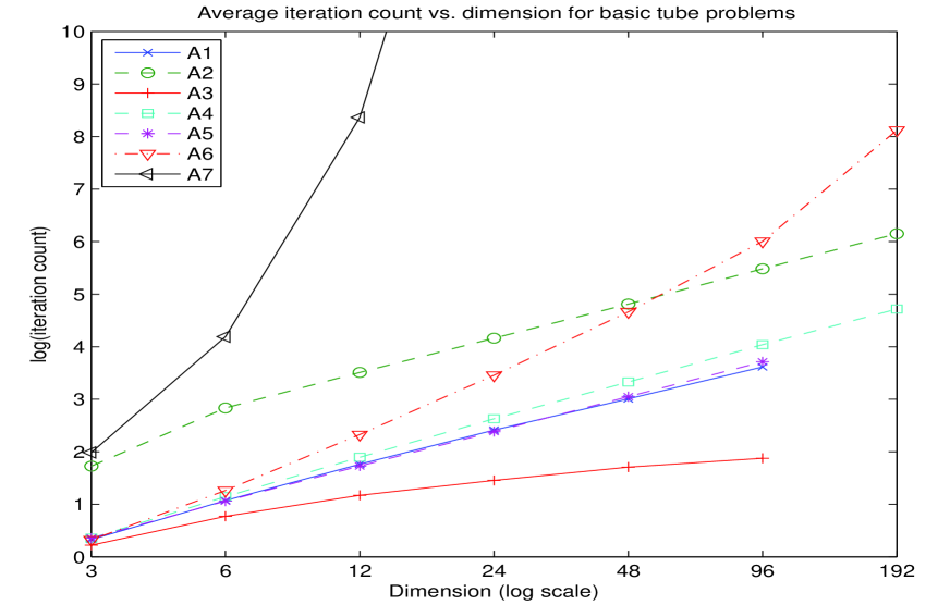
Figure 2. Results for G2.

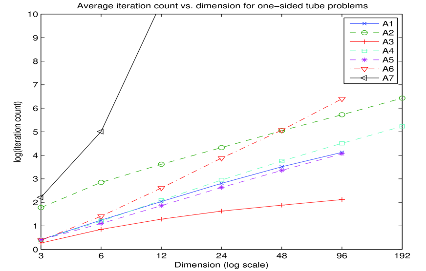
Figure 3. Results for G3.

The tube experiments summarized in Figures 2 and 3 show the impact of ill-conditioning on all the algorithms. For A1, A3, A5 and A6, convergence is slightly slower and numerical errors become more common. With these algorithms, our experiments began to crash at dimension 192. By contrast for the better conditioned problems from G1, the three algorithms with minimum distance calculations crashed only at dimension 384 and A6 would in any case take too long on problems of this size. Nevertheless, these algorithms remain effective at $d=96$.

The algorithms A2 and A4 are more robust in the sense that they are not as prone to crashes due to numerical errors. This is the advantage of relying entirely on straightforward linear algebra computations rather than considering nearest points or volumes. At the same time, they converge much more slowly due to problems of the type described in Section 6.2 and Appendix 6.2.

If we decrease the angle parameter which controls the width of the tube and hence the conditioning, the results become more pronounced. That is to say, A1, A3, A5 and A6 become less stable numerically and experience a further mild degradation in performance when not affected by numerical errors, while A2 and A4 become substantially slower.

We comment that the A7 algorithm performs about the same on G2 problems as it did on G1 problems. This simply means that G2 problems typically have a similar number of solutions to G1 problems. As one would expect, solutions to the one-sided tube problems generated by G3 are rarer than solutions to G1 and G2 problems since the most of the points are clustered on one side. Hence A7 performs much worse on this type of problem.

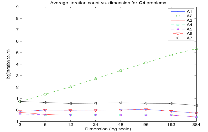
Figure 4. Results for G4.

The problems with many solutions produced by G4 are solved very quickly by all the algorithms, as illustrated in Figure 4. In this case the random sampling algorithm A7 offers excellent performance. With the abundance of solutions, most of the algorithms solve such problems in an expected constant number of iterations. The exception is A2 which needs $\Theta(d)$ iterations at the start to unwind the nearest point substitute $y$ from a vertex to an interior point on a facet. Since all the algorithms begin by checking the feasibility of the initial simplex, the G4 problems are often solved in 0 iterations.

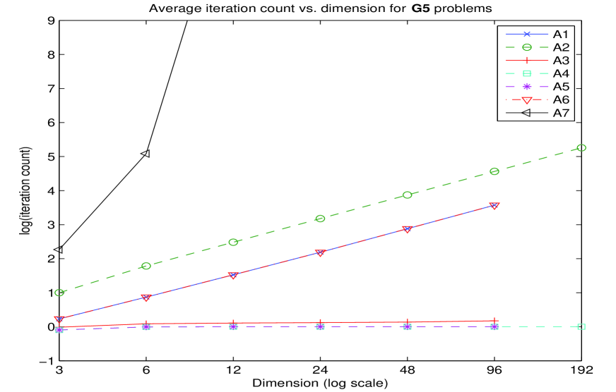
Figure 5. Results for G5.

For the simplex structured problems of G5, we see all the algorithms except A7 perform very well, despite the relative scarcity of solutions. We see that the other algorithms have exactly the proper response to this structure – they systematically take points near vertices that are not part of the current set. In the case of A1, a new vertex of the simplex will be added at each step to give convergence in at most $d$ iterations, for A2 it takes one pass through the $d+1$ colours, and for the multi-update algorithms A3, A4 and A5 one or two passes through the colours. Algorithm A6 also solves these problems in a reasonable number of iterations.

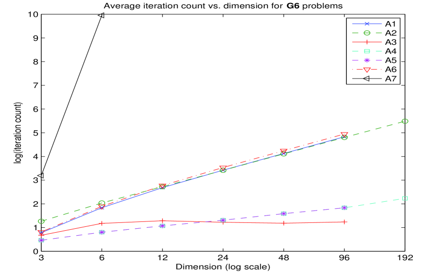
Figure 6. Results for G6.

Finally, we see that the problems from G6 where solutions are scarce are indeed more difficult than random problems, but that, except for the A7 algorithm, the impact on algorithmic performance is mild. See Figure 6. Curiously, the G6 problems are the most difficult problems for the A1 algorithm. The multi-update algorithms A3, A4 and A5 perform extremely well.

5.2. Cost per Iteration

In Figure 7 we present the average iteration times observed for all seven algorithms on problems from the G1 generator. The raw data for this graph is in Appendix D. We comment that the average time to complete an iteration does not change significantly with the problems type, so we have not included the similar graphs for other generators. The data shows that in our implementation of these algorithms, the average time for an iteration is never very large. For the slowest algorithms in the highest dimensions the average iteration took less than 2 seconds.

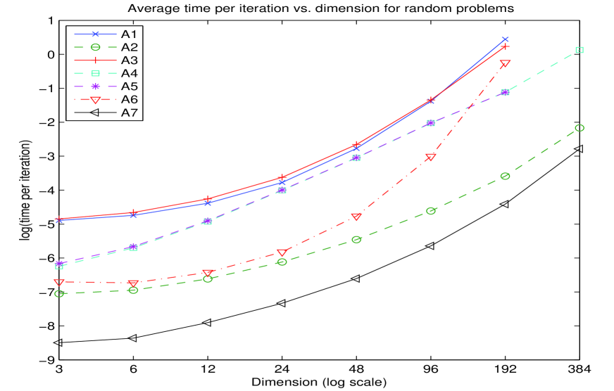
Figure 7. Average iteration time of the algorithms.

We see some interesting trends in the graphs. First, in low dimensions all the iteration times are very fast and are presumably dominated by fixed startup costs. As the dimension increases, we begin to see the asymptotic behaviour. The algebraic algorithms A2 and A4 show the expected $\Theta(d^{3})$ behaviour, which appears linear in the log-log plot. Asymptotically, the average time for an iteration of A4 is about 10 times longer for an iteration of A2.

The algorithms A1 and A3, which depend on a minimum distance calculation, take longer on average to complete an iteration than A4. The extra cost for the multiple updates in A3 is relatively small. However, the asymptotic slope of these lines appear higher than for A2, which means that the nearest point calculations are causing the iterations to take time $\Omega(d^{3})$. The algorithm A6 has iteration times not much worse than A2 in low dimension, but its asymptotics look close to $O(d^{4})$ as suggested in Section 3.6. Algorithm A7 exhibits $\Theta(d^{3})$ iteration time and is asymptotically about twice as fast on average per iteration than A2.

Unlike the other algorithms, the average iteration time for A5 will be substantially affected by the conditioning of the problem. Using the well-conditioned G1 problems, A5 usually degenerates to A4 and has a very similar average iteration time. As the problems become more ill-conditioned, A5 will begin to use A3 steps as well, and the average iteration time will increase towards the average iteration time for A3.

6. Conclusions

Our experiments reveal several features of colourful feasibility algorithms. After considerable searching, we found a problem instance which caused A6 to cycle. We also found that A2 and A4 can converge extremely slowly in the face of ill-conditioning although A1 and A3 continue to perform reasonably well on the same examples. We conclude that computationally the best algorithms are A3 and A4 and remark that these tightened algorithms do yield substantial gains over the originals.

6.1. A Cycling Example for A6 in Dimension 4

In Appendix A we exhibit an example in dimension 4 for which the maximum volume heuristic cycles. This example was found using our tube generator G2 to produce configurations where for each colour, four points are tightly bunched around (-1,0,0,0,0) and the fifth point is close to (1,0,0,0,0) or vice-versa. The example is fairly ill-conditioned, but not excessively so: we rounded the values we found for text formatting purposes, and observed that ${\bf 0}$ remained in the core and that the behaviour of the algorithm was unaffected.

Close examination of the iterations of this example turns up nothing out of the ordinary. Since this example shows that A6 can cycle, it is remarkable that it happens so rarely. It did not occur in the entire test suite of Section 5. We tested extensively in dimensions 3 and 4, and were unable to find any examples of cycling in dimension 3 or any examples of cycling in dimension 4 with cycle length shorter than 6. Higher dimensions and longer cycle lengths do occur.

One explanation for the results is that as one might expect, A6 is an effective heuristic in a typical situation. The distinguishing feature of the few bad examples is that the points are placed in such a way that the simplices cluster into a few groups of similar shape and volume. The heuristic of taking the maximum volume is then not very helpful in choosing promising simplices. We note that this example is solved easily by the other algorithms.

6.2. Flip-flopping During Convergence for A2: 40,847 Iterations in Dimension 3

We constructed an example of a colourful feasibility problem in dimension 3 that takes 40,847 iterations to solution using a basic implementation of A2. The exact points we used are contained in Appendix B. The algorithm is initialized with the simplex that uses the first point of each colour. At the fifth iteration, the algorithm reaches a situation where the current point $y$ lies on a facet $F$ of colours 2, 3 and 4 very close to ${\bf 0}$. Using this point the algorithm will pick the point of colour 1 that has minimum dot product with $y$. The second and third points of colour 1 lie almost in the directions of $y$ and $-y$, however neither of these forms a simplex with $F$ containing ${\bf 0}$. In fact the fourth point of colour 1 does form a simplex containing ${\bf 0}$ with $F$, but it is nearly orthogonal to $y$. As a result, after two iterations, A2 returns to the same simplex. The point $y$ will be recomputed at each step, and is slightly closer to ${\bf 0}$ when the algorithm returns to the previous simplex. However, the improvement is quite small. Of course $\rho$ is also very small, so this is consistent with the performance guarantee described in Section 3.2. The algorithm then proceeds to return to the same simplex more than 20,000 times, with an incremental improvement to $y$ at each iteration before finally taking the fourth point of colour 1 and terminating.

As one would expect with a very ill-conditioned problem, this example is numerically fragile – the current version of our code normalizes the coordinates before starting and does not suffer the same fate. However bad behaviour is fairly typical. The tube generator for ill-conditioned problems in [Hua] produces problems whose ill-conditioning depends on a parameter defining the width of the tube. As the width decreases, we get an increasing number of cases where A2 and A4 take enormous numbers of iterations.

We remark that, in contrast, A1 never returns to the same simplex, so it cannot suffer from this type of flip-flopping. Indeed in dimension 3 it could do no worse than visiting all $4^{4}=256$ simplices. At least 10 of these must contain ${\bf 0}$, see [BM05], so the algorithm must terminate in at most 246 iterations. It is quite hard to see how this limit could be approached. The authors wonder if a Klee-Minty-like example, see [KM72], of worst-case behaviour for Bárány’s pivoting algorithm could be constructed.

6.3. Overall Effectiveness of Algorithms

Despite the examples of Sections 6.1 and 6.2, the results presented in Section 5 show that, except for A7 and to a lesser degree A6, all the algorithms did a good job of solving all the problems. We did find that the methods which include nearest point calculations were more vulnerable to numerical errors than A2 and A4, since our implementations began to crash once we got much past $d=100$, especially on ill-conditioned problems. For the most part, reduced iteration counts of the nearest point algorithms do not offset the extra time spent per iteration compared to A2 and A4, since neither iteration count is very high. In some cases of extreme ill-conditioning, such as in Section 6.2, A2 and A4 will take many additional iterations and be much slower compared to the nearest point algorithms. In this situation either a hybrid algorithm such as A5, or the basic A1 or A3 would work better.

We had hoped that the hybrid algorithm A5 would offer the benefits of A4, namely speed and robustness in high dimensions, while stopping long periods of flip-flopping from occurring. This did happen to a degree, but in our benchmarking experiments the net time savings were negligible, while A5 retained A3’s tendency to crash due to numerical errors in high dimension.

6.4. Advantages of Multiple Updates and Initialization

The multi-update algorithms A3 and A4 do provide substantial gains over their single update counterparts, A1 and A2. In the case of A3, we get a large reduction in iteration count at very little cost in terms of iteration time. In our benchmarking experiments, this produced times that were competitive with A2 and much better than A1. The gains for A4 relative to A2 are less impressive. In our benchmarking experiments, A4 consistently averaged a 10% to 40% savings in total time to solution.

In fact, A2 is not as well suited as A1 to take advantage of multiple updates. The point $y$ close to ${\bf 0}$ computed by A2 will almost always lie in the interior of a facet of $\mathbf{\Delta}$, meaning that A2 will only have a single candidate colour to pivot. In contrast, in high dimension, the closest point $x$ to ${\bf 0}$ will often lie on a relatively low dimensional face of $\mathbf{\Delta}$, allowing multiple updates throughout the algorithm.

One difficulty for A2 is that it begins with $y$ at a vertex. In a normal situation, the first $d$ steps of A2 will each increase the dimension of the smallest face containing $y$ by one until $y$ lies in the interior of a facet, without necessarily yielding a much better current simplex. The multi-update A4 does this all in the first iteration in less time than it takes A2 to do $d$ steps.

We have not discussed the effects of the initial simplex in this paper, but we can employ various heuristics to choose a good initial simplex. A few of these are implemented in [Hua]. We found that the most useful initialization heuristic was to run the first iteration of A4. This runs in $O(d^{3})$ time and improves the subsequent iteration counts of the algorithms, with the obvious exception of A7. Even A4 experiences a reduced iteration count, since the point $y$ found by the initialization is not passed to the algorithm.

6.5. Theoretical Complexity of the Algorithms

In Section 3, we remarked that Bárány and Onn proved a worst-case bound for A1 and A2 of $O(1/\rho^{2})$ iterations up to numerical considerations and we improved their iteration time for A2 from $O(d^{4})$ to $O(d^{3})$. We also mentioned that we do not expect the multi-update and hybrid algorithms to improve the theoretical bounds. From the example of Section 6.1, we see that A6 is not guaranteed to converge. The expected running time of A7 is 1 over the probability that random simplex contains ${\bf 0}$, i.e. around $2^{d}$ for random problems, and as bad as $(d+1)^{d+1}/(d^{2}+1)$ for the type of problems generated by G6.

The poor performance of A2 on ill-conditioned problems and examples like that of Section 6.2 confirm the worst-case predictions of Bárány and Onn’s analysis. On the other hand, we did not see this type of behaviour for A1, and it is hard to see how it could occur.

The model proposed in Section 4.3 is that a pure pivoting algorithm such as A1, defines a set of rooted trees on the $(d+1)^{d+1}$ simplices. Each simplex which contains ${\bf 0}$ is the root of a tree, and we draw an edge between the vertices representing simplices $\mathbf{\Delta}_{1}$ and $\mathbf{\Delta}_{2}$ if when A1 encounters $\mathbf{\Delta}_{1}$ it pivots to $\mathbf{\Delta}_{2}$. Then the worst performance of the algorithm in terms of the number of iterations would be the height of the highest tree. A smart algorithm will produce short trees by pivoting several simplices to a given simplex at a lower level.

Consider a situation where trees have a constant expansion factor $k$ near the base, that is, low level vertices are connected to roughly $k$ vertices in the level above. The number of trees is $p(d+1)^{d+1}$ where $p$ is the probability that a simplex contains ${\bf 0}$. If the trees expand up to height $h$, each tree will contain on the order of $k^{h}$ vertices. Then we must have $k^{h}p(d+1)^{d+1}\leq(d+1)^{d+1}$, the total number of vertices. Rearranging, we get $h\leq-\log_{k}(p)$. This expression predicts the average iteration count for A1 to grow linearly for G1 problems, to be constant for G4 problems and to grow at $\Theta(d\log d)$ for G6 problems. All of these match very well with our observed results. The G5 problems are predicted to be more difficult than they are observed to be, but that is not surprising given their simple structure.

6.6. Future Considerations

We finish by returning to the motivating question of Bárány and Onn: Is there a polynomial time algorithm for colourful feasibility? By improving the implementation of A2, we have improved the worst case for this algorithm from $O(d^{4}/\rho^{2})$ to $O(d^{3}/\rho^{2})$, however the dependence on $\rho$ has not improved. Indeed our experiments give strong evidence that the analysis for A2 is tight.

The situation for A1 is less clear. We do not see the same bad behaviour with ill-conditioned problems that we found for A2, so it is possible that a better guarantee exists for this algorithm. In light of the model suggested in Section 6.5 it is quite difficult to see how to construct a Klee-Minty-like bad case for A1 as discussed in Section 6.2. We view this as an appealing challenge.

7. Acknowledgments

This research was supported by NSERC Discovery grants for the four authors, by the Canada Research Chair program for the first and last authors and by a MITACS grant for the second and third authors. The third author worked on this project as part of the Discrete Optimization project of the IMO at the University of Magdeburg.

Appendix A Example in dimension 4 where A6 cycles

This example consists of 5 normalized points in each of the 5 colours in $\mathbb{R}^{4}$. The points are presented in Table 1. They are grouped by colour, with the rows representing $x$, $y$, $z$ and $w$ coordinates, respectively.

Red points

-0.98126587	0.99234170	-0.99375618	-0.98428021	-0.99649986
0.13481464	0.01125213	-0.01676635	-0.03542019	0.03152825
0.00569666	-0.12300509	0.10203928	0.17121850	0.07625092
0.13751313	0.00104048	-0.04189897	0.02494182	-0.01340880

Green points

0.99924734	-0.99225276	0.95301586	0.99770745	0.98808067
0.03530047	-0.07048563	0.17760263	0.03405179	-0.00874509
-0.01500068	0.10036231	-0.24516979	-0.01526145	-0.12973853
0.00579663	-0.01984027	0.01048096	0.05645716	0.08238952

Blue points

-0.98758195	-0.99742900	-0.97286388	-0.97433105	0.99536963
-0.03897365	0.02836725	0.13575382	0.14413058	-0.06519965
-0.14957699	-0.06348104	-0.17638005	0.17286629	0.06380946
-0.02810110	-0.01734511	-0.06322067	-0.00475659	0.03027639

Tan points

0.99782436	0.99917562	0.95584087	-0.98768930	0.96962649
0.01692290	0.03972232	0.17806542	-0.10337937	0.14481818
0.03437294	-0.00816965	-0.21878711	0.09313650	-0.12491250
0.05365310	0.00186470	0.08242045	-0.07147128	0.15247636

White points

-0.99979855	-0.97268376	-0.97231627	-0.95622769	0.99791825
0.00600345	0.06950105	0.21172943	-0.29221243	-0.02997771
0.00415788	-0.00409898	-0.03733932	-0.01550644	0.01616939
0.01869548	0.22144776	0.09152860	0.00022801	-0.05476362

Table 1. Coordinates of points of an example where A6 cycles in dimension 4.

The initial simplex is taken to be (1,1,1,1,1), i.e., the first point of each colour. The algorithm proceeds to visit simplices (1,1,4,1,1), (3,1,4,1,1), (3,1,4,3,1), (3,1,1,3,1) and (1,1,1,3,1) before returning to the original simplex and repeating.

Appendix B Example in dimension 3 where A2 takes 40,847 iterations

This example consists of 4 unnormalized points in each of the 4 colours in $\mathbb{R}^{3}$. The points are presented in Table 2. They are grouped by colour, with the rows representing $x$, $y$ and $z$ coordinates, respectively.

Red points

1.00000320775369	-0.01000436049274	-0.01000129525998	1.00000089660284
0.00000340785030	0.99999739350954	-1.00000497855619	0.00000051797159
0.00999859615603	0.00000371775824	0.00000030149139	-0.01999639732055

Green points

1.00000363763560	-0.00999644886160	-0.00999943004295	1.00000335962280
-0.00000325123594	1.00000064545156	-1.00000169806216	-0.00000080450760
0.01000493174811	-0.00000024088601	0.00000009099437	-0.01999811804365

Blue points

0.99999949817337	-0.00999587145461	-0.00999627213896	0.99999551963712
-0.00000260397964	1.00000485455718	-1.00000419710665	-0.00000024626161
0.00999854691703	0.00000123671997	-0.00000381812529	-0.01999801526314

Tan points

0.99999980645233	0.10000000280522	-0.60000327600988	0.99999642880542
0.00000024487465	-0.98999719313413	0.79999695643245	-0.00000429109491
0.01000455311709	-0.00000405877812	0.00000372117690	-0.01000272055280

Table 2. Coordinates of points of an example taking 40,847 iterations of A2 in dimension 3.

The initial simplex is taken to be (1,1,1,1), i.e., the first point of each colour. It then updates to (1,3,1,1), (1,3,2,1), (1,3,2,3), (1,3,2,2) and reaches (3,3,2,2) on the fifth iteration. At this point, it begins to flip between (3,3,2,2) and (2,3,2,2) with $y$ initially alternating between values close to (0.2,$\pm$0.00200,0.00285). The values of all these coordinates decrease very slowly as the algorithm continues. At iteration 40,847 it chooses fourth point of colour 1 instead of the third. This makes the current simplex (4,3,2,2) which contains ${\bf 0}$.

Appendix C Iteration counts from our experiments

In this Appendix we present the raw data from our computational experiments. Each table presents results for a single random generator. The entries give the average number of iterations to solution for each algorithm at the given dimension. For each generator at $d=3$ we sampled 100,000 problems, at $d=6$ and $d=12$ we sampled 10,000 problems, at $d=24$ and $d=48$ we sampled 1,000 problems and finally for $d\geq 96$ we sampled 100 problems.

	A1	A2	A3	A4	A5	A6	A7
$d=3$	1.31	2.96	1.15	1.15	1.15	1.31	7.15
$d=6$	2.56	6.87	1.77	1.67	1.67	2.90	63.48
$d=12$	4.84	13.93	2.42	2.16	2.16	7.01	4133.15
$d=24$	8.84	27.70	3.07	2.87	2.87	19.07	Large
$d=48$	16.14	54.88	3.77	4.14	4.14	56.12	Large
$d=96$	28.80	108.71	4.26	6.39	6.39	185.57	Large
$d=192$	51.96	217.59	4.99	11.68	11.68	808.78	Large
$d=384$	Unstable	425.26	Unstable	21.63	Unstable	Large	Large

Table 3. Average iteration counts in G1 generator tests.

	A1	A2	A3	A4	A5	A6	A7
$d=3$	5	136	4	4	4	5	102
$d=6$	7	21	5	5	5	12	579
$d=12$	10	30	6	6	6	20	47362
$d=24$	15	37	6	8	8	43	Large
$d=48$	22	67	6	9	9	105	Large
$d=96$	39	120	6	10	10	269	Large
$d=192$	63	241	7	19	19	1574	Large
$d=384$	Unstable	472	Unstable	30	Unstable	Large	Large

Table 4. Maximum iteration counts found in G1 generator tests.

	A1	A2	A3	A4	A5	A6	A7
$d=3$	1.39	5.62	1.25	1.43	1.43	1.38	7.30
$d=6$	2.92	17.00	2.17	3.14	2.89	3.54	66.02
$d=12$	5.83	33.48	3.23	6.65	5.64	10.26	4296.66
$d=24$	11.18	64.30	4.29	13.86	10.86	31.75	Large
$d=48$	20.24	123.02	5.51	27.91	21.11	106.11	Large
$d=96$	37.12	240.49	6.54	56.70	40.91	406.10	Large
$d=192$	Unstable	468.52	Unstable	111.84	Unstable	3367.60	Large
$d=384$	Unstable	909.82	Unstable	220.50	Unstable	Large	Large

Table 5. Average iteration counts in G2 generator tests.

	A1	A2	A3	A4	A5	A6	A7
$d=3$	5	4783	4	5	5	6	109
$d=6$	8	2880	6	44	10	14	1079
$d=12$	13	842	8	60	14	33	78418
$d=24$	21	217	9	36	23	78	Large
$d=48$	31	249	9	55	41	258	Large
$d=96$	47	323	9	77	76	840	Large
$d=192$	Unstable	561	Unstable	140	Unstable	11784	Large
$d=384$	Unstable	1013	Unstable	260	Unstable	Large	Large

Table 6. Maximum iteration counts found in G2 generator tests.

	A1	A2	A3	A4	A5	A6	A7
$d=3$	1.51	5.93	1.31	1.51	1.51	1.48	9.16
$d=6$	3.48	17.26	2.35	3.31	3.01	4.10	150.31
$d=12$	7.64	37.22	3.62	8.06	6.43	13.61	Large
$d=24$	16.59	75.73	5.11	19.11	13.92	48.51	Large
$d=48$	33.51	155.48	6.57	42.81	28.70	159.29	Large
$d=96$	61.97	306.64	8.32	90.98	58.44	602.07	Large
$d=192$	Unstable	619.55	Unstable	186.86	Unstable	Large	Large
$d=384$	Unstable	1221.43	Unstable	382.10	Unstable	Large	Large

Table 7. Average iteration counts in G3 generator tests.

	A1	A2	A3	A4	A5	A6	A7
$d=3$	6	2756	5	6	6	6	127
$d=6$	9	3704	7	38	9	14	1709
$d=12$	16	689	8	55	16	46	Large
$d=24$	28	195	9	52	27	124	Large
$d=48$	50	257	10	83	47	505	Large
$d=96$	78	374	11	133	83	2023	Large
$d=192$	Unstable	736	Unstable	226	Unstable	Large	Large
$d=384$	Unstable	1399	Unstable	454	Unstable	Large	Large

Table 8. Maximum iteration counts found in G3 generator tests.

	A1	A2	A3	A4	A5	A6	A7
$d=3$	0.89	2.07	0.82	0.71	0.71	0.89	2.12
$d=6$	0.99	3.96	0.68	0.66	0.66	0.99	1.94
$d=12$	0.97	7.61	0.63	0.63	0.63	0.97	1.78
$d=24$	0.99	15.46	0.64	0.64	0.64	0.99	1.83
$d=48$	1.01	31.15	0.65	0.65	0.65	1.01	1.87
$d=96$	1.06	61.44	0.64	0.64	0.64	1.06	1.81
$d=192$	0.90	122.88	0.64	0.64	0.64	0.90	1.77
$d=384$	0.77	211.20	0.55	0.55	0.55	0.77	1.50

Table 9. Average iteration counts in G4 generator tests.

	A1	A2	A3	A4	A5	A6	A7
$d=3$	2	5	2	3	3	2	38
$d=6$	3	7	2	2	2	3	17
$d=12$	6	12	1	1	1	6	30
$d=24$	6	24	1	1	1	6	19
$d=48$	5	48	1	1	1	5	16
$d=96$	5	96	1	1	1	5	14
$d=192$	3	192	1	1	1	4	15
$d=384$	4	384	1	1	1	4	9

Table 10. Maximum iteration counts found in G4 generator tests.

	A1	A2	A3	A4	A5	A6	A7
$d=3$	1.26	2.72	0.99	0.91	0.91	1.26	9.67
$d=6$	2.39	5.97	1.09	0.99	0.99	2.39	161.93
$d=12$	4.61	12.00	1.12	1.00	1.00	4.61	Large
$d=24$	8.94	24.00	1.13	1.00	1.00	8.94	Large
$d=48$	17.82	48.00	1.15	1.00	1.00	17.82	Large
$d=96$	35.58	96.00	1.19	1.00	1.00	35.58	Large
$d=192$	71.15	192.00	1.47	1.00	1.00	71.15	Large

Table 11. Average iteration counts in G5 generator tests.

	A1	A2	A3	A4	A5	A6	A7
$d=3$	3	5	3	2	2	3	128
$d=6$	5	6	3	1	1	5	1371
$d=12$	9	12	3	1	1	9	Large
$d=24$	14	24	2	1	1	14	Large
$d=48$	24	48	2	1	1	24	Large
$d=96$	41	96	2	1	1	41	Large
$d=192$	81	192	3	1	1	81	Large

Table 12. Maximum iteration counts found in G5 generator tests.

	A1	A2	A3	A4	A5	A6	A7
$d=3$	2.19	3.54	1.96	1.59	1.59	2.26	24.39
$d=6$	6.27	7.67	3.24	2.23	2.23	6.65	21041.05
$d=12$	14.64	15.23	3.63	2.92	2.92	16.03	Large
$d=24$	30.55	30.42	3.40	3.71	3.71	34.25	Large
$d=48$	61.96	60.95	3.27	4.89	4.89	69.65	Large
$d=96$	125.31	121.73	3.45	6.26	6.26	140.79	Large
$d=192$	Unstable	242.06	Unstable	9.31	Unstable	Unstable	Large

Table 13. Average iteration counts in G6 generator tests.

	A1	A2	A3	A4	A5	A6	A7
$d=3$	5	7	5	4	4	6	242
$d=6$	12	15	7	6	6	12	173941
$d=12$	25	25	8	9	9	25	Large
$d=24$	47	49	9	13	13	51	Large
$d=48$	101	94	13	22	22	95	Large
$d=96$	154	174	6	35	35	183	Large
$d=192$	Unstable	331	Unstable	69	Unstable	Unstable	Large

Table 14. Maximum iteration counts found in G6 generator tests.

Appendix D Average time per iteration

In Table 15 we give the average CPU time per iteration for our G1 experiments. This was computed using the MATLAB cputime function.

	A1	A2	A3	A4	A5	A6	A7
$d=3$	0.0075	0.0009	0.0078	0.0019	0.0021	0.0012	0.0002
$d=6$	0.0087	0.0010	0.0095	0.0033	0.0035	0.0012	0.0002
$d=12$	0.0124	0.0013	0.0141	0.0073	0.0074	0.0016	0.0004
$d=24$	0.0229	0.0022	0.0267	0.0182	0.0184	0.0030	0.0007
$d=48$	0.0625	0.0043	0.0702	0.0474	0.0477	0.0085	0.0014
$d=96$	0.2510	0.0099	0.2608	0.1318	0.1324	0.0495	0.0035
$d=192$	1.5592	0.0277	1.2623	0.3275	0.3268	0.7843	0.0121
$d=384$	Unstable	0.1144	Unstable	1.1381	Unstable	Unstable	0.0619

Table 15. Average iteration times on G1 generator tests.

The time per iteration is fairly constant across problem types so we do not include data from the other generators. One difference that will occur is that A5 will have a higher average iteration time as that A4 for ill-conditioned problems. In random problems, we rarely see slow convergence of A4 so it is unnecessary to use the slower steps from A3. With ill-conditioned problems the A3 steps become more frequent and increase the average time per iteration.

References

- [Bár82] I. Bárány, A generalization of Carathéodory’s theorem, Discrete Math. 40 (1982), no. 2-3, 141–152.
- [BM05] I. Bárány and J. Matoušek, Quadratically many colorful simplices, submitted, 2005.
- [BO97] I. Bárány and S. Onn, Colourful linear programming and its relatives, Math. Oper. Res. 22 (1997), no. 3, 550–567.
- [DHST05] A. Deza, S. Huang, T. Stephen, and T. Terlaky, Colourful simplicial depth, Discrete Comput. Geom. (2005), To appear. arXiv:math.CO/0506003
-
[Hua]
S. Huang, MATLAB code for colourful linear programming, available
at:
http://optlab.mcmaster.ca/~huangs3/CLP/ and
http://www.math.uni-magdeburg.de/~stephen/Software/CLP/. - [KM72] V. Klee and G. J. Minty, How good is the simplex algorithm?, Inequalities III, Proc. 3rd Symp., Los Angeles 1969, Academic Press, 1972, pp. 159–175.
- [ST05] T. Stephen and H. Thomas, A quadratic lower bound for colourful simplicial depth, in preparation, 2005.
- [WW01] U. Wagner and E. Welzl, A continuous analogue of the upper bound theorem, Discrete Comput. Geom. 26 (2001), no. 2, 205–219.