The process of most recent common ancestors
in an evolving coalescent

Abstract

Consider a haploid population which has evolved through an exchangeable reproduction dynamics, and in which all individuals alive at time $t$ have a most recent common ancestor (MRCA) who lived at time $A_{t}$, say. As time goes on, not only the population but also its genealogy evolves: some families will get lost from the population and eventually a new MRCA will be established. For a time-stationary situation and in the limit of infinite population size $N$ with time measured in $N$ generations, i.e. in the scaling of population genetics which leads to Fisher-Wright diffusions and Kingman’s coalescent, we study the process $\mathcal{A}=(A_{t})$ whose jumps form the point process of time pairs $(E,B)$ when new MRCAs are established and when they lived. By representing these pairs as the entrance and exit time of particles whose trajectories are embedded in the look-down graph of Donnelly and Kurtz (1999) we can show by exchangeability arguments that the times $E$ as well as the times $B$ from a Poisson process. Furthermore, the particle representation helps to compute various features of the MRCA process, such as the distribution of the coalescent at the instant when a new MRCA is established, and the distribution of the number of MRCAs to come that live in today’s past.

1 Introduction

The genealogy back to the most recent common ancestor (MRCA) of those currently alive, and especially the time back to the MRCA, has been an ongoing object of interest in mathematical population genetics, see [Lit75], [Gri80] for early references and [Wak05] for a recent monograph. The limit of effective population size $N\to\infty$, with time measured in units of $N$ generations, is the scaling in which Kingman’s coalescent appears ([Kin82]): in the rescaled time measured backward from a fixed time $t$, the number of ancestral lineages enters from infinity and jumps from $k$ to $k-1$ at rate $\binom{k}{2}$. (Here and below we assume that the population size remains constant in time.) The depth $D_{t}$ of the coalescent tree, that is the rescaled time it takes the number of ancestral lineages to decrease from $\infty$ to $1$, is then a sum of exponentially distributed random variables with mean ${\binom{k}{2}}^{-1}$, $k=2,3,\ldots$, and consequently has expectation $2$.

With the population evolving further, also its genealogical relationships given by the coalescent tree change. In this study we are interested in the time evolution of one particular characteristics of the genealogy, that is, the time $A_{t}=t-D_{t}$ when the MRCA of the population at time $t$ lived. We will refer to $\mathcal{A}=(A_{t})_{t\in\mathbb{R}}$ as the MRCA process.

At any time $t$ the total population consists of two oldest families, which stem from the two oldest lines of descent dating back to the MRCA who lived at time $A_{t}$. These two families will coexist for a while after time point $t$, and during this time interval the path of the MRCA process $\mathcal{A}$ stays constant. At some random time $E_{t}>t$, one of the two families will go extinct and the other one will fixate in the population. The MRCA of this surviving family must be more recent than $A_{t}$, which amounts to a jump of the MRCA process at time $E_{t}$. Consequently, at time $E_{t}$, the next MRCA is established, and the time when this next MRCA lives is $B_{t}:=A_{E_{t}}$. In other words, the path of the process $\mathcal{A}$ is constant as long as the two currently oldest families coexist in the population, and jumps from $A_{t}$ to $B_{t}$ at time $E_{t}$ when one of the two families fixates.

The MRCA process is embedded in the genealogy of the population which is assumed to evolve in a time stationary way. For a finite population consisting of $N$ individuals, a way to construct the genealogy comes with the graphical representation of the Moran model: for each ordered pair $(i,j)$ of indices $i\neq j\in\{1,..,N\}$, an exponential clock rings at rate $1/2$, and whenever this happens, the individual with index $j$ dies and is replaced by an offspring of the individual with index $i$. This results in a partitioning of $\mathbb{R}\times\{1,\ldots,N\}$ into coalescing ancestral lineages, from which one can read off a version of the MRCA process for $N$ individuals. This process clearly inherits time stationarity from the evolution of the population.

The Moran dynamics is exchangeable with respect to the individuals’ indices. In contrast, the look-down process introduced by Donnelly and Kurtz (1999), which is the basic tool in our study and will be reviewed in Section 2, arranges the individuals’ indices (henceforth referred to as levels) at any time according to the persistence of the individuals’ offspring in the population: the offspring of an individual at level $i$ outlives the offspring of any contemporary individual at some higher level. For a finite population number $N$ this is achieved as follows: Each level $j$ “looks down” to each smaller level $i$ at rate 1. Whenever this happens, all individuals at levels $j,\ldots,N-1$ are pushed one level up, the individual at level $N$ is killed, and the individual at level $i$ spawns a child at level $j$. The time stationary MRCA process read off from the look-down graph obviously has the same distribution as the time stationary MRCA process read off from the Moran graph.

The look-down process allows a passage to the limit of infinite population size in which the ordering by persistence is preserved. The construction of the random look-down graph on $\mathbb{R}\times\mathbb{N}$ proceeds in the very same way as described above, except that there is no killing of individuals at any finite level. Instead, the offspring of an individual at level $i\geq 2$ goes to extinction as soon as this line of ascent of the individual is pushed to infinity. All this will be explained in more detail in Section 2.

Because of the ordering by persistence, each MRCA of the population lives at level 1 at some time $B$ at which it gives birth to an individual at level 2. As soon as the offspring of these two individuals fixates in the population, the MRCA is established. Again, because of the ordering by persistence, this happens at the time $E$ when the line of ascent which was pushed at time $B$ from level 2 to level 3 reaches infinity. The process $\mathcal{F}:=\{(E,B)\}$, which consists of all pairs of time points when an MRCA is established in the population and when it lived, is a time-stationary point process; we call it the MRCA point process. The paths of $\mathcal{A}$ and the point configurations of $\mathcal{F}$ are in an obvious one-to-one correspondence.

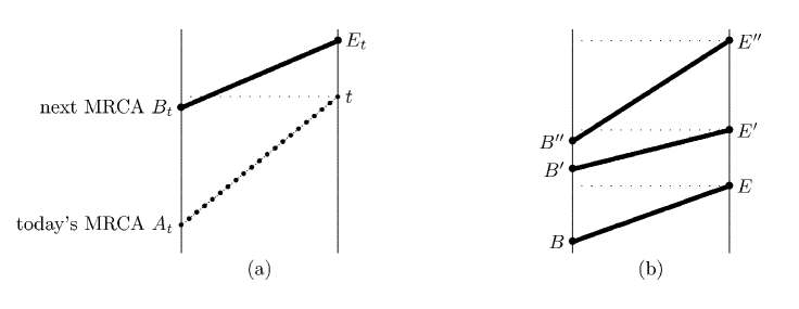
Figure 1: (a) At time $A_{t}$ the MRCA of the population at time $t$ lived, $E_{t}$ and $B_{t}$ are the times when the next MRCA is established and when it lived.  (b) MRCAs occur in a time-stationary manner. The dots on the $B$-axis are time points at which MRCAs lived. The dots on the $E$-axis are time points at which the MRCA changes.

The step from time $t$ to the next MRCA, which is established at time $E_{t}$ and lives at time $B_{t}$, and an illustration of the MRCA point process $\mathcal{F}$ are depicted in Figures 1(a) and 1(b) respectively. In both Figures, the left axis contains the times when MRCAs live, and the right axis gives the times when MRCAs are established. The joint distribution of $E_{t}$ and $B_{t}$ will be given in Theorem 1 in Section 3. Figure 1(b) displays part of the MRCA point process $\mathcal{F}$. Remarkably, not only the points $B$ but also the points $E$ form a time stationary Poisson process, see Theorem 2 in Section 4. This will be proved by representing the times $(B,E),(B^{\prime},E^{\prime}),\ldots$ as the entrance and exit times of particles: the trajectory of a particle is attached to the line of ascent which is pushed from level 2 to level 3 at time $B$ and exits at time $E$. We will specify the Markovian dynamics of this particle system, compute its equilibrium distribution and show that, whenever a particle exits at some time $E$, at this very instant the system of (remaining) particles is in equilibrium. This allows to conclude that the waiting time to the next exit time is exponential. The processes $\mathcal{A}$ and $\mathcal{F}$, however, are not Markov, see Remark 4.1.3.

In Theorem 3 we compute the distribution of the random number $Z_{t}=\#\{(E,B)\in\mathcal{F}\,|\,E>t,B<t\}$ of MRCAs that are established after time $t$ and live before time $t$. In particular, it turns out that the probability that the next MRCA lives in today’s future is $\mathbf{P}[Z_{t}=0]=1/3$.

As noted by [Taj90], the amount of polymorphism in a population is related to the fixation of alleles. When an allele fixates, the MRCA of the population must have changed. At such a fixation time, the full coalescent is unusually short. As neutral mutations fall independently on the branches of the genealogical tree, this means that the amount of polymorphism is low at fixation times.

We start out by reviewing the look-down process in Section 2, describe our results in Sections 3 and 4, point out some relations to population genetics in Section 5 and give the proofs of Theorems 1-3 in Sections 6–8.

2 The MRCA process: a look-down construction

At every time a continuum population which follows a Wright-Fisher (or Fleming-Viot) dynamics has a genealogy given by Kingman’s coalescent. The look-down process introduced by Donnelly and Kurtz ([DK99]) not only gives a countable representation of evolving allele frequencies but at the same time stores genealogical relationships of all the individuals alive in the population at all times. Consequently the MRCA process can be read off from the look-down process.

The look-down graph: ancestral lineages, lines of ascent and ordering by persistence

We first give a brief review of the “modified look-down process” ([DK99]); see Figure 2 for a graphical illustration.

Consider the set of vertices

$$\mathcal{V}:=\mathbb{R}\times\mathbb{N}.$$

We will refer to the vertex $(t,i)$ as the individual at time $t$ at level $i$. For each ordered pair of levels $i<j$, let $\mathcal{P}_{ij}$ be the support of a (rate one) Poisson point process on $\mathbb{R}$, all these processes being independent. (In the terminology of Donnelly and Kurtz, at each time $t\in\mathcal{P}_{ij}$, the level $j$ looks down to level $i$.) Based on the processes $\mathcal{P}_{ij}$ we will construct a random countable partition $\mathcal{G}$ of $\mathcal{V}$, whose partition elements will be called lines. The partition $\mathcal{G}$ will always contain the so-called immortal line $\iota$ defined by

$$\iota:=\mathbb{R}\times\{1\}.$$ (2.1)

For each $j>1$, any point $s_{0}\in\bigcup_{i}\mathcal{P}_{ij}$ initiates a line $G\in\mathcal{G}$ of the form

$$G=([s_{0},s_{1})\times\{j\})\cup([s_{1},s_{2})\times\{j+1\})\cup([s_{2},s_{3})\times\{j+2\})\cup\ldots$$ (2.2)

with $s_{k+1}>s_{k}$ for all $k$. For a line $G$ as in (2.2) with $s_{0}\in\mathcal{P}_{ij}$ we say that $G$ is born at level $j$ by the individual $(s_{0},i)$. We further say that $G$ is pushed (one level up) at times $s_{1},s_{2},\ldots$ and exits at time $s_{\infty}(G):=\lim_{n\to\infty}s_{n}$. The times $s_{k}$ are given for $k=1,2,\ldots$ by $s_{k}=\inf\{s>s_{k-1}:s\in\bigcup_{1\leq\ell<m\leq j+k-1}\mathcal{P}_{\ell m}\}$. Thus, a new line is born at level $j$ at each time $t$ when level $j$ looks down to some level $i<j$. Simultaneously, all the lines having occupied at time $t-$ the levels $j,j+1,\ldots$ are pushed one level up. Note that, since the pushing rate increases quadratically in $j$, the exit time $s_{\infty}(G)$ is finite a.s.

For each $v\in\mathcal{V}$, we denote by $G_{v}$ the (unique) element of $\mathcal{G}$ that contains $v$. The forward level process $Y_{s}^{t}(i),\,t\geq s$, initiated by the individual $u=(s,i)$ is given by

$$Y_{s}^{t}(i):=\mbox{ level of }G_{u}\mbox{ at time }t.$$

The line of ascent of individual $u=(s,i)$ is the part of line $G_{u}$ after time $s$, that is

$$(t,Y_{s}^{t}(i))_{s\leq t<s_{\infty}(g)}.$$

We say that a line $H$ descends from a line $G$ if either $H=G$, or there is a finite sequence of lines $G_{1},\ldots,G_{n-1}\in\mathcal{G}$ such that $G_{k}$ is born by an individual in $G_{k-1}$ , $k=1,\ldots,n$, where $G_{0}:=G$ and $G_{n}:=H$.

The backward level process $X_{s}^{t}(j),\,s\leq t$, of an individual $v=(t,j)$ arises by tracing back the level of $G_{v}$ to the birth time of $G_{v}$, then jumping to the level of the individual $u$ from which $G_{v}$ was born and tracing back the level of $G_{u}$ to the birth time of $(s,i)$, and so on.

The ancestral lineage of the individual $v=(t,j)$ is

$$(s,X_{s}^{t}(j))_{-\infty<s\leq t}\;;$$

note that eventually all ancestral lineages coalesce with the immortal line.

We say that an individual $v\in\mathcal{V}$ descends from an individual $u\in\mathcal{V}$ (or equivalently, $u$ is an ancestor of $v$) if $u$ belongs to the ancestral lineage of $v$. The random tree spanning $\mathcal{V}$ which is obtained in this way is the random look-down graph.

Let $u=(s,i)$ and $v=(s,j)$ be two individuals living at the same time $s$, with $i<j$. By construction the line of ascent of $v$ is pushed whenever the line of ascent of $u$ is pushed, hence $Y_{s}^{t}(i)<Y_{s}^{t}(j)$, and the line of ascent of $v$ exits not later than that of $u$. In this sense, the ordering of lines by contemporaneous levels is an ordering by persistence. Note also that for all times $s<t$ and all levels $i\in\mathbb{N}$:

$$Y_{s}^{t}(i)=\inf\{j\in\mathbb{N}:X_{s}^{t}(j)=i\}.$$

Thus, the time when an individual’s line of ascent reaches infinity marks the time at which the individual’s offspring goes extinct.

Let us note in passing that the ordering by persistence is a main distinction between the version of the look-down process developed in [DK99] and its precursor introduced in [DK96]. In the latter, the order by persistence is only stochastic, that is, lines of ascent of contemporaneous individuals at lower levels are longer “in probability”. In the modified look-down process of [DK99], explained and employed in the present paper, this property holds almost surely.

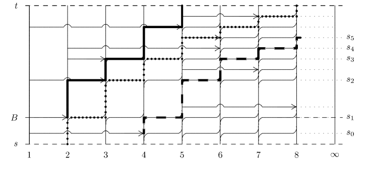
Figure 2: Detail of a look-down graph. Time is running upwards; all lines at the first 8 levels are drawn between times $s$ and $t$. At times in $\mathcal{P}_{ij}$ an arrow is drawn from $i$ to $j$. All lines at levels at and above $j$ are pushed upwards as indicated by bent lines. The solid marked line is the fixation curve $F_{B}^{\tau},\tau\geq B$. The dotted line is the coalescent curve $C_{\tau}^{t}(8),\tau\leq t$. The dashed line is the line born at level 4 by the individual $(s_{0},1)$; it is pushed one level up at times $s_{1},s_{2},\ldots$. In this picture, $X_{s}^{t}(1)=\ldots=X_{s}^{t}(5)=X_{s}^{t}(7)=1$ and $X_{s}^{t}(6)=X_{s}^{t}(8)=2$; $Y_{s}^{t}(1)=1,Y_{s}^{t}(2)=6,Y_{s}^{t}(3)>8$; $C_{s}^{t}(1)=\ldots=C_{s}^{t}(5)=1$ and $C_{s}^{t}(6)=\ldots=C_{s}^{t}(8)=2$.

Coalescent curves and fixation curves

For $t\in\mathbb{R}$ and $i\in\mathbb{N}$ the coalescent tree $\mathfrak{C}^{t}(i)$ consists of the ancestral lineages of the individuals $(t,1),,(t,i)$, i.e. $X_{s}^{t}(1),\ldots,X_{s}^{t}(i)$ for $s\leq t$, whereas the full coalescent tree $\mathfrak{C}^{t}$ is made up of the ancestral lineages of all individuals living at time $t$. All these lineages eventually coalesce with the immortal line. Since any pair of ancestral lineages coalesces at rate 1, $\mathfrak{C}^{t}(i)$ and $\mathfrak{C}^{t}$ are distributed like Kingman’s (finite respectively infinite) coalescent. The number of lineages remaining at time $s<t$ can be expressed as

$$C_{s}^{t}(i):=\max\{X_{s}^{t}(1),...,X_{s}^{t}(i)\},\qquad C_{s}^{t}:=C_{s}^{t}(\infty):=\sup_{i\in\mathbb{N}}C_{s}^{t}(i).$$ (2.3)

In words, $C_{s}^{t}(i)$ is the number of time $s$-ancestors of the time $t$-individuals at levels $1,\ldots,i$, and $C_{s}^{t}$ is the number of time $s$-ancestors of the whole population at time $t$. For fixed $t$, we call $(C_{s}^{t})_{s\leq t}$ the coalescent curve in the look-down graph back from time $t$. It is distributed like the death process in Kingman’s coalescent entering from infinity.

The time when the MRCA of the total population at time $t$ lived is

$$A_{t}:=\sup\{s:C_{s}^{t}=1\}.$$

All individuals at time $t$ descend either from individual $(A_{t},1)$ or from individual $(A_{t},2)$. At time $A_{t}$ a line must be born at level $2$, which is equivalent to $A_{t}\in\mathcal{P}_{12}$. Denote the next point in $\mathcal{P}_{12}$ after $A_{t}$ by $B_{t}$:

$$B_{t}:=\min\{s\in\mathcal{P}_{12}:s>A_{t}\}.$$

The offspring of the two individuals $(B_{t},1),(B_{t},2)$ evolves towards fixation in the population by pushing the line of ascent of the individual $(B_{t},3)$ towards infinity. The time $E_{t}$ when this line of ascent exits equals the time when the offspring of the individual $(A_{t},2)$ is expelled by the offspring of $\{(B_{t},1),(B_{t},2)\}$. Thus the time $E_{t}$ is the first time after $t$ when a new MRCA is established, and the time when this MRCA lives is $B_{t}$.

Note that at any time $\tau$ between $B_{t}$ and $E_{t}$, all the levels $1,\ldots,Y_{B}^{\tau}(3)-1$ are occupied by offspring of $\{(B_{t},1),(B_{t},2)\}$, whereas level $Y_{B}^{\tau}(3)$ is not. We therefore call

$$F_{B_{t}}^{\tau}:=Y_{B_{t}}^{\tau}(3)-1=Y_{A_{t}}^{\tau}(2)-1,\quad B_{t}\leq\tau<E_{t},$$ (2.4)

the fixation curve starting in time $B_{t}$. (For the equality in (2.4), note that the line containing $(B_{t},3)$ was born at time $A_{t}$ at level 2 and was pushed to level 3 at time $B$.) When $Y_{B_{t}}^{\tau}(3)=k$ the corresponding line moves to $k+1$ at the next look-down event among the first $k$ levels, i.e. at rate $\binom{k}{2}$. As a consequence, $F_{B_{t}}^{\tau}$ is pushed from level $k$ to level $k+1$ at rate $\binom{k+1}{2}$.

The MRCA point process $\mathcal{F}$ records all the time points when the fixation curves start and end. We will pursue this in Section 4, by constructing an autonomous particle system whose trajectories give the fixation curves.

Whereas the coalescent curves are constructed from any $t$ backwards in time, the fixation curves start only at points in $\mathcal{P}_{12}$ and are constructed forwards in time.

At a time $E$ when a fixation curve ends (and a new MRCA is established), all individuals descend from the MRCA who lived at the time $B$ when this fixation curve started. Hence the fixation curve between time points $B$ and $E$ equals the coalescent curve back from time $E$. With time proceeding, the coalescent curve evolves, being more and more “zipped away” from the upper end of the fixation curve (near time point $E$), and still sharing the lower part (near time point $B$) for a while.

Having now constructed the process $\mathcal{A}$ in terms of the look-down graph, we will study its properties in the next sections.

3 From today to the next MRCA

As in the previous section, $A_{t}$ denotes the time when the current MRCA lived, $E_{t}$ is the time when the next MRCA is established and $B_{t}=A_{E_{t}}$ is the time when the next MRCA lives. In this section we will compute the conditional distribution of $(E_{t},B_{t})$ given $A_{t}$.

The following random variables will play a crucial role:

$$L_{t}:=F_{B_{t}}^{t}\,,$$ (3.1)

the level at time $t$ of the fixation curve starting at time $B_{t}$, and

$$I_{t}:=C_{B_{t}}^{t}\,,$$ (3.2)

the level at time $B_{t}$ of the coalescent curve back from time $t$, where we define

$$L_{t}:=1\mbox{ and }I_{t}:=\infty\mbox{ on the event }\{B_{t}>t\}.$$

Without loss of generality, and to ease notation, let us put $t=0$, and write $L:=L_{0},I:=I_{0},E:=E_{0},B:=B_{0}$.

Note that, because of the ordering by persistence, the lines of ascent starting at time $0$ from levels $1,\ldots,L$ exit only after time $E$, whereas the lines starting at time $0$ from levels $L+1,L+2,\ldots$ exit at time $E$ or earlier. Thus, $L$ is the random number of individuals in the present population that still have offspring when the next MRCA is established.

Proposition 3.1.

The pair $(L,I)$ is independent of $A_{0}$ and has distribution

$$\mathbf{P}[L=\ell,I=i]=\begin{cases}\displaystyle\frac{\ell-1}{3\binom{\ell+i}{\ell}},&\ell\geq 2,i\geq 3\\ \tfrac{1}{3},&\ell=1,i=\infty\\ 0,&\text{else.}\end{cases}$$ (3.3)

Proposition 3.1 will be proved in Section 6.

Remark 3.2.

1. Summing over $i$ in (3.3) leads to the distribution of $L$:

   $$\mathbf{P}[L=\ell]=\frac{2}{(\ell+1)(\ell+2)},\quad\ell=1,2,\ldots$$ (3.4)

   Since $\{L=1\}=\{B>0\}$ is the event that that first fixation curve which ends after time $0$ has not yet started by time $t=0$. we infer that the probability that the next MRCA lives in today’s future is

   $$\mathbf{P}[B>0]=\mathbf{P}[L=1]=1/3.$$

2. Here is another quick way to (3.4), exploiting exchangeability. Recall that the number $L$ gives the number of lines that still have offspring at the time when the next MRCA is established. At any time there are two oldest families in the population. The family sizes of these two oldest families, denoted by $P$ and $1-P$, evolve according to a Wright-Fisher diffusion. It is well known (and can be understood from the Pólya urn scheme embedded in the genealogy; see e.g. facts about the Pólya-Eggenberger distribution in [JK77], eq. (4.1)) that, at any fixed time, say at time $t=0$, $P$ is uniformly distributed on $[0,1]$. This also remains true conditioned on the event $A_{0}^{\infty}=-d$. By exchangeability, the probability that the first $\ell$ most persistent lines are in one and the $(\ell+1)$-st most persistent line is in the other family is

   $$\mathbf{P}[L=\ell]=2\int_{0}^{1}p^{\ell}(1-p)dp=2\Big{(}\frac{1}{\ell+1}-\frac{1}{\ell+2}\Big{)}=\frac{2}{(\ell+1)(\ell+2)}.$$ (3.5)

To prepare for Theorem 1, we need one more bit of notation.

Definition 3.3.

Let $T_{k}$ be independent exponentially distributed random variables with parameter $\binom{k}{2}$, $k=2,3,\ldots$, and

$$S_{i}^{j}=\sum_{k=i+1}^{j}T_{k},\qquad 1\leq i<j\leq\infty.$$

For $d>0$ and $i=1,2,..$ let $R_{i,d}$ be a random variable whose distribution equals the conditional distribution of $S_{i}^{\infty}$ given that $S_{1}^{i}+S_{i}^{\infty}=d.$

The random variable $S_{i}^{j}$ represents the time which Kingman’s coalescent requires to come down from $j$ to $i$. Consequently, $R_{i,d}$ refers to the random time for a coalescent to come down from infinity to $i$ lines, given that coming down to 1 line requires exactly time $d$. Note also that $S_{i}^{j}$ represents the time a fixation curve needs to be pushed from level $i$ to level $j$. This can be seen because a fixation curve goes from level $\ell$ to level $\ell+1$ whenever a look-down event among the first $\ell+1$ levels occurs, i.e. with rate $\binom{\ell+1}{2}$.

We are now prepared to state Theorem 1, which together with Proposition 3.1 yields the desired conditional distribution of $(E,B)$ given $A_{0}$.

Theorem 1.

Let $L$ and $I$ be as in (3.1) and (3.2). The conditional distribution of $(E,B)$, given $A_{0}=-d$, $L=\ell$ and $I=i$ is represented by the random variables

$$\begin{cases}(S_{1}^{2}+S_{2}^{\infty},S_{1}^{2})&\mbox{ if }\ell=1,\\[8.61108pt] (S_{\ell}^{\infty},-R_{i,d})&\mbox{ if }\ell>1,\end{cases}$$ (3.6)

where $(S_{\ell}^{j})$ and $R_{i,d}$ have the distribution specified in Definition 3.3, and $R_{i,d}$ and $S_{\ell}^{\infty}$ are independent.

The proof of Theorem 1 is given in Section 6.

Remark 3.4.

1. Combining (3.6) and (3.4) we obtain

   $$\mathbf{P}[E\in ds\big{|}A_{0}=d]=\sum_{\ell=1}^{\infty}\frac{2}{(\ell+1)(\ell+2)}\mathbf{P}[S_{\ell}^{\infty}\in ds],\qquad s\geq 0.$$ (3.7)

   From this one can conclude that the conditional distribution of $E$ given $A_{0}$ is standard exponential. Indeed, think of a 2-sample (i.e. a subsample of size two) embedded in a full coalescent. The coalescence time of this 2-sample is standard exponentially distributed. Denoting by $L^{\prime}$ the number of lineages remaining in the full coalescent at the time when the 2-sample has found its common ancestor, one sees from [GT03], eq. (2.10) or [STW84], Lemma 3, or by direct calculation, that $L^{\prime}$ has the same distribution as $L$ specified in (3.4) and (3.5). This shows that the r.h.s. of (3.7) is a decomposition of the standard exponential distribution.

2. Here is another quick (though slightly informal) argument that the waiting time to the next jump of the MRCA is exponential, independently of the depth of the current MRCA. Note first that, conditioned on $A_{0}=-d$ the split of the population size into the two oldest families at time $t=0$ is uniformly distributed on $[0,1]$. As a consequence, given the MRCA does not jump during the time interval $[0,s]$, the split remains uniformly distributed also at time $s$. (This corresponds to the fact that the uniform distribution is a quasi-equilibrium for the Wright-Fisher diffusion.) At the next jump of the MRCA process one of the two oldest families dies out. After the jump there will be two families inside the surviving family that again make up a uniform split. This implies that the time between jumps proceeds in a memoryless manner, showing that the conditional distribution of $E_{0}$ given $A_{0}$ is exponential.

   Notably, the fact of exponential waiting times between the jumps can also be read from (3.10) in [Wat82a]. See Section 5 for comments relating to this paper and to other applications.

4 A particle representation of the MRCA point process

The set $\mathcal{G}$ of lines defined in Section 2 randomly partitions the set $\mathcal{V}=\mathbb{R}\times\mathbb{N}$. Let us write

$$\mathcal{G}_{2}:=\{G\in\mathcal{G}\,\big{|}\,G\mbox{ is born at level }2\}.$$

For each line $G\in\mathcal{G}_{2}$ we write $B:=B(G)$ for the time when $G\in\mathcal{G}_{2}$ is pushed from level 2 to level 3 (due to the birth of the next line in $\mathcal{G}_{2}$) and $E:=E(G)$ for the exit time of $G$. Thus we obtain a one-to-one correspondence between $\mathcal{G}_{2}$ and the sequence of fixation curves by associating with any $G\in\mathcal{G}_{2}$ the fixation curve $F_{B}$ starting at time $B$ and ending at time $E$. This fixation curve is related to the level path of $G$ by $F_{B}^{\tau}=Y_{B}^{\tau}(3)-1$ for $B\leq\tau<E$; see (2.4). The MRCA point process $\mathcal{F}$ then can be written as

$$\mathcal{F}=\{(E,B)\,\big{|}\,G\in\mathcal{G}_{2}\}.$$

Additionally, we write

$$\eta:=\{E\,|\,(E,B)\in\mathcal{F}\}\qquad\text{ and }\qquad\eta_{t}:=\eta\cap(-\infty,t]$$

for the exit time point process and its restriction to $(-\infty,t]$ respectively.

In this section we will gain more information about the processes $\mathcal{F}$ and $\eta$ by interpreting the fixation curves as the trajectories of an interacting particle system on $\{2,3,4,\ldots\}$ whose dynamics and equilibrium distribution we will compute.

Let

$$Z_{t}:=\#\{(E,B)\in\mathcal{F}\,\big{|}\,E>t,B<t\}.$$

In other words, $Z_{t}$ is the number of fixation curves present at time $t$, that is, the number of MRCAs which will be established after time $t$ and have lived before time $t$.

Write

$$L_{t}^{1}>L_{t}^{2}>\ldots>L_{t}^{Z_{t}}>1$$ (4.1)

for the levels of the fixation curves at time $t$. Let us interpret $(L_{t}^{1},L_{t}^{2},\ldots,L_{t}^{Z_{t}})$ as a configuration of particles on the set of levels $\{2,3,4,\ldots\}$ at time $t$, and put

$$\Lambda_{t}:=(L_{t}^{1},L_{t}^{2},\ldots),\qquad\Lambda:=(\Lambda_{t}),$$

where $L_{t}^{j}:=1$ for $j>Z_{t}$. The first components in the MRCA point process $\mathcal{F}$ are the exit times of the “leading particles”, i.e. those time points $E$ where $\lim_{t\uparrow E}L_{t}^{1}=\infty$. Whenever a particle exits, the indices of all remaining particles are shifted down by one:

$$(L_{E}^{1},L_{E}^{2},\ldots):=(L_{E-}^{2},L_{E-}^{3},\ldots).$$ (4.2)

Here is a verbal description of the dynamics of the particle system (see Proposition 7.1 for a formal statement): Particles are pushed in at level 2 at rate 1, each particle at level $\ell\geq 2$ is pushed one level up at rate $\binom{\ell+1}{2}$, and this is done in a coupled way such that, whenever a particle is pushed, all particles at higher levels are pushed simultaneously. The next theorem specifies the equilibrium distribution of $\Lambda$. We will see that this distribution prevails also in the distinguished random time points $E$ where $\lim_{t\uparrow E}L_{t}^{1}=\infty$. This property is crucial to see that $\eta$ is a Poisson process.

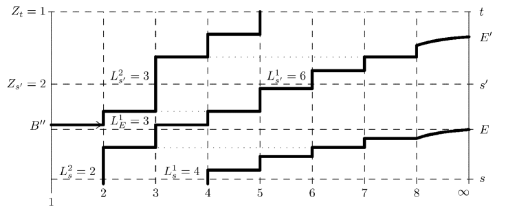
Figure 3: The embedding of the fixation curves in the look-down process. At times $B$ fixation curves start and at times $E$ they end. In this example, at time $s$ the number of particles in the system is $Z_{s^{\prime}}=2$, the leading particle being at level $6$, and the second particle at level $2$.

Theorem 2.

1. The process $\Lambda=(\Lambda_{t})$ is Markov with stationary distribution

   $$\pi_{\Lambda}(\ell_{1},\ell_{2},\ldots)=\begin{cases}\displaystyle\frac{1}{3}\prod_{j:\ell_{j}>1}\frac{2}{(\ell_{j}+2)(\ell_{j}-1)},&\ell_{k}>\ell_{k+1},\quad\text{ if }\ell_{k}>1,\\ 0,&\text{else}.\end{cases}$$ (4.3)

   In particular, the stationary distribution of $L^{1}$ is

   $$\pi_{L^{1}}(\ell)=\frac{2}{(\ell+1)(\ell+2)}.$$ (4.4)

2. The process of exit times $\eta$ is a stationary Poisson process.

Remark 4.1.

1. The “arrival time points” $B$ of the particles in the system $\Lambda$ (the times when the MRCAs live) are the points of the stationary Poisson process $\mathcal{P}_{12}$. Theorem 2 states that also the “departure time points” $E$ (the times when the MRCAs are established) form a stationary Poisson process. Thus, the Poisson input process of times $B$ when the fixation curves begin is transformed by a “dependent stochastic shift” into the Poisson output process of times $E$ when they end. This is similar to Burke’s theorem which states that the departure process in a time stationary $M/M/1$ queue is Poisson, see [Kur98] and references given there. A crucial property (proved already by Burke (1956)) is that in a stationary $M/M/1$ queue the distribution of the queue length at time $t$ is independent of the departure times $\leq t$. In the language of queueing theory, our particles correspond to customers entering at the time points of a stationary Poisson process, and the time which a typical customer spends in the system is distributed like $S_{2}^{\infty}$ specified in Definition 3.3. These times are mutually dependent. As the proof of Theorem 2 reveals, like in Burke’s theorem the state of the system (now given by the configuration $\Lambda_{t}$ of particles at time $t$) does not depend on the departure times $\leq t$.

2. We recently learned from Tom Kurtz about the manuscript [DK06] where he and Peter Donnelly have established the filtered martingale problem for the $N$-level analogue of the pair $(\Lambda,\eta)$ in the context of [Kur98], Theorem 3.2 and thus achieved an alternative proof of the fact that the “MRCA fixation process” $\eta$ is Poisson.

3. Whereas the particle process $\Lambda$ is Markov, the MRCA process $\mathcal{A}$ is not. This can be seen as follows:

   

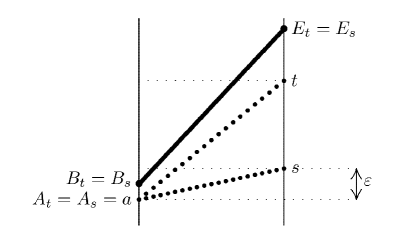
   Figure 4: Assume we know $A_{t}=A_{s}=a$ for some $s=a+\varepsilon$. This knowledge leads to a higher chance of the MRCA time $B_{t}$ falling between times $a$ and $s$ than in an equilibrium situation. This shows that the future of the process $\mathcal{A}$ at time $t$ depends on the past and $\mathcal{A}$ cannot be Markov. See text for explanation.

   Let $a,s,t$ be as in Figure 4. Conditioned on $A_{t}=a$ we obtain from Theorem 1:

   $$\mathbf{P}[B_{t}<s|A_{t}=a]=\mathbf{P}[R_{I,t-a}>t-s]\xrightarrow{s\downarrow a}0.$$

   On the other hand, we claim that $\mathbf{P}[B_{t}<s|A_{t}=A_{s}=a]$ does not converge to zero as $s\downarrow a$, which shows that $\mathcal{A}$ cannot be Markov. To verify the claim, we write, using Bayes’ rule

   $$\mathbf{P}[B_{t}<s|A_{t}=A_{s}=a]=\frac{\mathbf{P}[B_{s}<s,A_{t}=A_{s}|A_{s}=a]}{\mathbf{P}[A_{t}=A_{s}|A_{s}=a]}.$$

   By Theorem 1, the denominator converges to $e^{-(t-a)}$ as $s\downarrow a$. Likewise, the numerator is bounded away from $0$ as $s\downarrow a$, a trivial lower bound being

   $$\mathbf{P}[L_{s}=2]\,\mathbf{P}[S_{2}^{3}\geq t-s]=\frac{1}{6}e^{-3(t-s)}\geq\frac{1}{6}e^{-3(t-a)}.$$

4. The level $L_{t}^{1}$ of the leading particle in (4.1) coincides with $L_{t}$ defined in (3.1). Thus we recover (3.4) from (4.4).

Recall from (4.1) that

$$Z_{t}=\max\{j\in\mathbb{N}\,\big{|}\,L_{t}^{j}>1\},$$

where $\max\emptyset:=0$. Consequently,

$$\{Z_{t}=0\}=\{L_{t}^{1}=1\}.$$

This is the event that there is no particle on $\{2,3,4,..\}$ at time $t$, or equivalently, that all fixation curves starting before time $t$ also end before $t$. Given this event, the fixation curves starting before time $t$ are independent of those starting after $t$.

In a way, the random variable $Z_{t}$ of MRCAs that are established in today’s future and live in today’s past measures the dependence between past and future in the MRCA process. Note also that because of Theorem 3 the distribution of $Z_{t}$ does not change when $t$ is conditioned to be the time of an MRCA change.

In the next theorem we calculate the equilibrium distribution of $Z:=Z_{t}$.

Theorem 3.

1. The probability generating function of $Z$ is

   $$\mathbf{E}[u^{Z}]=\frac{1}{3}\exp\Big{(}\sum_{i=2}^{\infty}\log\Big{(}\frac{i(i+1)+2(u-1)}{(i+2)(i-1)}\Big{)}.$$

2. The expectation and variance are

   $$\mathbf{E}[Z]=1,\qquad\mathbf{Var}[Z]=14-\tfrac{4}{3}\pi^{2}\approx 0.84052.$$

3. The probability weights are given by

   $$\mathbf{P}[Z=z]=\frac{2^{z}}{3}\sum_{\underline{a}:\sum ia_{i}=z}(-1)^{z+\sum a_{i}}\frac{1}{a_{1}!\cdots a_{z}!}\prod_{j=1}^{z}\Big{(}\frac{x_{j}}{j}\Big{)}^{a_{j}},\qquad(z\geq 0)$$

   where the $a_{i}\in\mathbb{N}_{0}$ and

   $$x_{k} :=\frac{(-1)^{k+1}}{3^{2k-1}}\sum_{j=1}^{k}\binom{2k-j-1}{k-j}3^{j-1}\big{(}b_{j}-1_{\{j\;\rm{even}\}}2\zeta(j)\big{)},$$ (4.5)

   $$\zeta(k) :=\sum_{j=1}^{\infty}\frac{1}{j^{k}},$$

   $$b_{j} :=1+\frac{1}{2^{j}}+\frac{1}{3^{j}}.$$

4. The weights for $z=0,1,2,3$ are

   $$\mathbf{P}[Z=0] =\frac{1}{3}, \mathbf{P}[Z=1] =\frac{11}{27}\approx 0.40740,$$

   $$\mathbf{P}[Z=2] =\frac{107}{243}-\frac{2}{81}\pi^{2}\approx 0.19664, \mathbf{P}[Z=3] =\frac{1003}{2187}-\frac{10}{243}\pi^{2}\approx 0.05246.$$

5 Relations to population genetics

Consider sequence data, obtained from a sample of individuals in a population that reproduces according to Wright-Fisher dynamics. Besides resampling we consider neutral mutations for an infinite sites model (as introduced in [Kim71]) occurring at rate $\theta/2$ along each line. Using common notation in population genetics, we consider the diffusion limit of the dynamics of the population, where time has been rescaled by a factor $N$, the number of haploids in the population. The per generation mutation probability of $\mu$ along each line is rescaled to $\theta/2$, where $\theta=2N\mu$.

Mutations can also be modelled in the look-down picture: for each level there is an independent Poisson clock with rate $\theta/2$ by which mutations on the line carrying the corresponding level accumulate. This implies that on each line of the lookdown process mutations arise at rate $\theta/2$. All mutations an individual carries at time $t$ are collected along its line of descent.

Segregating sites

For two individuals sampled from the population, the expected number of segregating sites is $\theta\mathbf{E}[T_{c}]$, where $T_{c}$ is the random time to coalescence of the individuals’ ancestral lineages. This time is unusually short at instances when the MRCA changes. In [Taj90], Tajima studied the coalescent at such times. He concluded that then the coalescence rate from $k$ to $k-1$ ancestral lineages is $\binom{k+1}{2}$, his argument being that, in addition to the $k$ lineages, there is one extra line, which apparently must belong to the family that disappears at the time of the MRCA change.

These coalescence rates can also be seen from the particle representation of the MRCA process. In fact, the fixation curves give the shape of the coalescent tree of the whole population back from the time of the MRCA change. Recall that the fixation curve moves from level $k$ to $k+1$ at rate $\binom{k+1}{2}$. Consequently the time the coalescent back from some time point $E$ stays with $k$ lines is exponentially distributed with rate $\binom{k+1}{2}$, which means that this is the rate to go down from $k$ to $k-1$ lineages. As these rates differ from the rates in Kingman’s coalescent the random coalescence time $T_{c}$ of the 2-sample cannot be exponential. However, the 2-sample coalescent is embedded in the full coalescent; the probability that the two sampled lines find a common ancestor at the time when there are $\ell$ lines left in the full coalescent is (see Remark 3.4 or [Taj90], equation (6))

$$\frac{2}{(\ell+1)(\ell+2)}.$$

As the time of going down from infinity to $\ell$ lines in the coalescent at an MRCA time is distributed like $S_{\ell+1}^{\infty}$, we obtain the distribution for the coalescence time $T_{c}$ of the two lines

$$\mathbf{P}[T_{c}\in dt]=\sum_{\ell=1}^{\infty}\frac{2}{(\ell+1)(\ell+2)}\mathbf{P}[S_{\ell+1}^{\infty}\in dt].$$

Taking expectations we obtain

$$\mathbf{E}[T_{c}] =\sum_{\ell=1}^{\infty}\frac{2}{(\ell+1)(\ell+2)}\frac{2}{\ell+1}=4\sum_{\ell=1}^{\infty}\Big{(}\frac{1}{(\ell+1)^{2}}-\frac{1}{(\ell+1)(\ell+2)}\Big{)}=\tfrac{2}{3}\pi^{2}-6\approx 0.58,$$

a result already obtained in [Taj90]. As the coalescence time for two lines in equilibrium is exponential with mean 1, this result means that the expected number of segregating sites for a 2-sample is reduced by $42\%$ at times when the MRCA changes.

For samples of arbitrary size, the number of segregating sites is Poisson with mean $\theta/2$ times the total branch length of the sample’s genealogical tree. In [RBY04], Figure 2c, a path of the time evolution of this total branch length is depicted for a spatial and a “well-mixed” population. At certain instances, one sees sudden substantial decrease of the path length. One may guess that this happens primarily at times at which the MRCA changes, since then the coalescent tree is unusually short.

Substitutions

Most mutations that occur in a population are quickly lost. However, some eventually fixate, i.e. all individuals in the population carry the new mutation. This replacement is termed a substitution and the corresponding mutations are called determining mutations. In [Wat82a] and [Wat82b], Watterson studied several aspects of the process of substitutions. While we are concerned with the jump from today’s MRCA to the next one, Watterson fixes two time points $0$ and $t$ and studies the time between the MRCAs at these times, i.e. $A_{t}-A_{0}$, irrespectively of the number of MRCAs that are established between $0$ and $t$. All mutations on the ancestral line between $A_{t}$ and $A_{0}$ are then determining mutations and their number gives the the number of substitutions between times $0$ and $t$.

The only way a mutation can become a substitution is through an MRCA change. This is because any mutation that occurs in the population belongs to one of the two oldest families. For the mutation to become fixed it is necessary that the family not carrying the mutation dies out. In other words, it is necessary that the MRCA changes.

Consider the graphical lookdown representation including mutations falling on lines at all levels at rate $\theta/2$. A mutation that occurs is determining if and only if it occurs on the line at level one. Indeed, we already found that MRCAs of the population as seen in the lookdown picture always are at level one. On the other hand, given the time point of a mutation on a line at level one, eventually all individuals in the population are descendants of the individual carrying this mutation which shows that all mutations that occur at level one are determining.

Denote by $\mathcal{S}=\{(\tilde{E},S)\}$ the process of times $\{\tilde{E}\}$ and number $\{S\}$ of substitutions at these times. As times $E$ of MRCA changes are the only ones that can be substitution times and the number of mutations on a line is Poisson distributed with rate $\tfrac{\theta}{2}$ we find that the process $\mathcal{S}$ is a close relative to the MRCA point process:

Proposition 5.1.

Let $\{(E,B)\}$ be distributed as the MRCA point process. Additionally, for all successive pairs $(E^{\prime},B^{\prime})$ and $(E^{\prime\prime},B^{\prime\prime})$, let $S^{\prime\prime}$ be Poisson-distributed with intensity parameter $\tfrac{\theta}{2}(B^{\prime\prime}-B^{\prime})$. Then $\{(E^{\prime\prime},S^{\prime\prime}):S^{\prime\prime}>0\}$ is a version of $\mathcal{S}$.

This confirms the observation in [Wat82b] that (i) substitution times do not form a Poisson process and (ii) substitutions tend to occur in clusters.

6 Proof of Theorem 1

Recall the definition of $L_{t}$ and $I_{t}$ in (3.1) and (3.2), and also recall that we put without loss of generality $t=0$, omitting the corresponding sub-and superscripts $0$. By definition, the fixation curve $F_{B}$ starts at time $B$ at level $2$ and exits at time $E$ at level $\infty$; let us now extend this definition by putting

$$F_{B}^{\tau}:=1\quad\mbox{ if }\tau<B.$$

The following auxiliary variables will be helpful:

$$K^{j}:=\mbox{ the level of }F_{B}\mbox{ while }C=j,\qquad j=2,3,\ldots$$

and

$$I^{k}:=\mbox{ the level of }C\mbox{ when }F_{B}\mbox{ reaches level }k,\qquad k=2,3,\ldots$$

Formally, putting

$$\tau_{k}:=\inf\{\tau:F_{B}^{\tau}=k\},\quad k=2,3,..$$

we have

$$I^{k}=\begin{cases}C_{\tau_{k}},&\text{ if }\tau_{k}<0,\\ \infty,&\text{ if }\tau_{k}\geq 0.\end{cases}$$

Thus, $\tau_{2}=B$, $I^{2}=I$,

$$K^{j}=\max\{k:I^{k}\leq j\}\quad\text{ and }\quad L=K^{\infty}:=\lim_{j\to\infty}K^{j}.$$ (6.1)

The random variables $I^{k}$, $K^{j}$ and $L$ are illustrated in Figure 5.

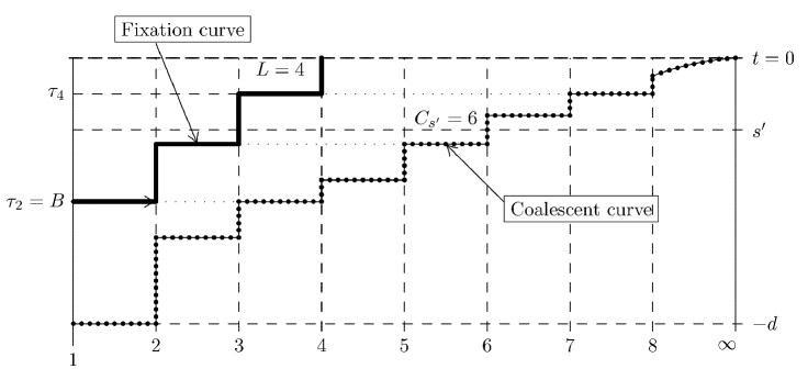
Figure 5: The variable $I^{k}$ is the level of the coalescence curve back from time $t=0$ when the next fixation curve has reached level $k$. The corresponding real times are denoted by $\tau_{k}$. The variable $K^{j}$ is the level of the fixation curve when the coalescent curve has reached level $j$. In this example, $I^{2}=4$, $I^{3}=6$, $I^{4}=8$, $K^{2}=K^{3}=1,K^{4}=K^{5}=2,K^{6}=K^{7}=3$ and $K^{8}=4$.

Lemma 6.1.

$K=(K^{2},K^{3},\ldots)$ is an inhomogeneous Markov chain starting in $K^{2}=1$ and with transition probability given by

$$\mathbf{P}[K^{j+1}=k+1|K^{j}=k]=\frac{\binom{k+1}{2}}{\binom{j+1}{2}}=1-\mathbf{P}[K^{j+1}=k|K^{j}=k],\quad j>k\geq 1.$$ (6.2)

Moreover, $K$ is independent of the coalescence curve $C$.

Proof.

When the coalescence curve moves from $j+1$ to $j$ at some time $s$, that is, $C_{s}=j+1$ and $C_{s-}=j$, then some look-down event involving two levels $\leq k+1$ must happen. When at time $s-$ the fixation curve is at level $k$, the probability that the fixation curve jumps at time $s$ from $k$ to $k+1$ is $\binom{k+1}{2}/\binom{j+1}{2}$, since all possible look-down events are equally probable and there are $\binom{\ell+1}{2}$ events that push the next fixation curve one level up. Observe that this is independent of the prehistory $K^{2},\ldots,K^{j-1}$, independent of the coalescence curve $C$, and in particular also independent of the time $A_{0}$. ∎

In the next lemma we calculate the joint distribution of the random variables $I^{k}$.

Lemma 6.2.

The joint distribution of $(I^{2},I^{3},\ldots)$ is given by

$$\mathbf{P}[I^{2}=\ldots=\infty] =\frac{1}{3},$$ (6.3)

$$\mathbf{P}[I^{2}=i_{2},\ldots,I^{\ell}=i_{\ell},I^{\ell+1}=\ldots=\infty] =\frac{\ell!(\ell-1)!}{3}\prod_{m=2}^{\ell}\frac{1}{(i_{m}+m)(i_{m}+m-1)}$$ (6.4)

for $2<i_{2}<\ldots<i_{\ell}.$

Proof.

The event $\{I^{2}=\infty\}$ equals the event that the next fixation curve has not yet started by time 0, that is the event $\{B>0\}=\{K_{j}=1\mbox{ for all }j=1,2,\ldots\}$. Thus, using (6.2),

$$\mathbf{P}[I^{2}=\infty] =\prod_{j=3}^{\infty}\Big{(}1-\frac{1}{\binom{j}{2}}\Big{)}=\prod_{j=3}^{\infty}\frac{(j+1)(j-2)}{j(j-1)}=\frac{1}{3},$$

since the product telescopes. This shows (6.3). To prove (6.4), we express the event on its left hand side in terms of the variables $K^{j}$:

$$\{I^{2}=i_{2},\ldots,I^{\ell}=i_{\ell},I^{\ell+1}=\ldots=\infty\}$$

$$=\{K^{2}=\ldots=K^{i_{2}-1}=1,\ldots,\,K^{i_{\ell-1}}=\ldots=K^{i_{\ell}-1}=\ell-1,\,K^{i_{\ell}}=K^{i_{\ell}+1}=\ldots=\ell\}.$$

Putting $i_{1}=2$ and $i_{\ell+1}=\infty$, and using Lemma 6.1 we arrive at

$$\mathbf{P} [I^{2}=i_{2},\ldots,I^{\ell}=i_{\ell},I^{\ell+1}=\infty]=\left[\prod_{m=1}^{\ell}\prod_{j=i_{m}+1}^{i_{m+1}-1}\Big{(}1-\frac{\binom{m+1}{2}}{\binom{j}{2}}\Big{)}\right]\cdot\left[\prod_{m=1}^{\ell-1}\frac{\binom{m+1}{2}}{\binom{i_{m+1}}{2}}\right]$$

$$=\ell!(\ell-1)!\left[\prod_{m=1}^{\ell}\prod_{j=i_{m}+1}^{i_{m+1}-1}\frac{(j-m-1)(j+m)}{j(j-1)}\right]\left[\prod_{m=1}^{\ell-1}\frac{1}{(i_{m+1})(i_{m+1}-1)}\right]$$

$$=\ell!(\ell-1)!\left[\prod_{m=1}^{\ell-1}\frac{(i_{m}-m)\cdots(i_{m}-1)}{(i_{m+1}-m-1)\cdots(i_{m+1}-2)(i_{m+1}-1)}\right.$$

$$\left.\qquad\qquad\qquad\qquad\qquad\qquad\qquad\frac{i_{m+1}\cdots(i_{m+1}+m-1)}{(i_{m}+1)\cdots(i_{m}+m)i_{m+1}}\right]\cdot\frac{(i_{\ell}-\ell)\cdots(i_{\ell}-1)}{(i_{\ell}+1)\cdots(i_{\ell}+\ell)}$$

$$=\frac{\ell!(\ell-1)!}{3}\frac{1}{(i_{\ell}+\ell)(i_{\ell}+\ell-1)}\left[\prod_{m=2}^{\ell-1}\frac{1}{(i_{m}+m)(i_{m}+m-1)}\right]$$

$$=\frac{\ell!(\ell-1)!}{3}\prod_{m=2}^{\ell}\frac{1}{(i_{m}+m)(i_{m}+m-1)}$$

∎

From the joint distribution of $I^{2},I^{3},\ldots$ given in Lemma 6.2 we obtain because of (6.1) the joint distribution of $(L,I)$ by projection:

Proof of Proposition 3.1

Because of $\{L=1\}=\{I^{2}=\infty\}$, we obtain the assertion of (3.3) for $\ell=1$ from (6.3). For $\ell=2,3,..$ we proceed by induction. For $\ell=2$ we have, using again Lemma 6.2,

$$\mathbf{P}[I=i,L=2]=\mathbf{P}[I^{2}=i,I^{3}=\infty]=\frac{2}{3}\frac{1}{(i+2)(i+1)}.$$

If the assertion is true for all $2,\ldots,\ell$, we have

$$\mathbf{P}[I=i,\, L=\ell+1]=\sum_{i<i_{3}<\ldots<i_{\ell+1}}\mathbf{P}[I^{2}=i,I^{3}=i_{3},\ldots,I^{\ell+1}=\ell+1,I^{\ell+2}=\infty]$$

$$=\frac{1}{(i+2)(i+1)}\sum_{i<i_{3}<\ldots<i_{\ell+1}}\frac{(\ell+1)!\ell!}{3}\prod_{m=3}^{\ell+1}\frac{1}{(i_{m}+m)(i_{m}+m-1)}$$

$$=\frac{(\ell+1)\ell}{(i+2)(i+1)}\sum_{i<j}\frac{1}{(j+3)(j+2)}\sum_{j+1<i_{3}<\ldots<i_{\ell}}\frac{\ell!(\ell-1)!}{3}\prod_{m=3}^{\ell}\frac{1}{(i_{m}+m)(i_{m}+m-1)}$$

$$=\frac{(\ell+1)\ell}{(i+2)(i+1)}\sum_{i<j}\mathbf{P}[I=j+1,L=\ell]=\frac{(\ell+1)!\ell(\ell-1)}{3(i+2)(i+1)}\sum_{i<j}\frac{1}{(j+2)\cdots(j+\ell+1)}$$

$$=\frac{(\ell+1)!\ell}{3(i+2)(i+1)}\sum_{i<j}\frac{1}{(j+2)\cdots(j+\ell)}-\frac{1}{(j+3)\cdots(j+\ell+1)}$$

$$=\frac{(\ell+1)!\ell}{3(i+2)(i+1)}\frac{1}{(i+3)\cdots(i+\ell+1)}$$

and we are done. ∎

We turn now to the

Completion of the Proof of Theorem 1

Given $\{L=1\}=\{B>0\}$, and independently of $C$ (and therefore also of $A_{0}$), the time $B$ it takes to enter the next fixation curve is standard exponentially distributed (and therefore distributed like $S_{1}^{2}\sim\exp(1)$), and the additional time it takes this fixation curve to exit is distributed like $S_{2}^{\infty}$, and is independent of $B$.

Given $L=\ell\geq 2$, $I=i<\infty$ and $A_{0}=-d$, the time at which the coalescent curve jumps from level $i+1$ to $i$ is distributed like $-R_{i,d}$. By construction, this is also the time $B$ at which the next fixation curve $F_{B}$ enters. At time $0$, this fixation curve is at level $\ell$; independently of the past, the time it takes until this fixation curve exits is distributed like $S_{\ell}^{\infty}$. $\Box$

7 Proof of Theorem 2

First we give a formal description of the dynamics of the process $\Lambda$. Afterwards we derive its equilibrium distribution, and finally we show that this equilibrium distribution also prevails at the distinguished times $E$.

The dynamics of $\Lambda$

Assume $Z_{t}=k$ with $L_{t}^{1}=\ell_{1},\ldots,L_{t}^{k}=\ell_{k}>L_{t}^{k+1}=1$, i.e. at time $t$ there are exactly $k$ particles at levels $>1$; in other words, exactly $k$ fixation curves are present at time $t$. Assume level $j$ looks down to level $i$ for $i<j$. If $j>\ell_{1}+1$ only lines at level greater than $\ell_{1}+1$ are pushed. In this case no particle moves, i.e. $L_{t}$ stays constant. When $j\leq\ell_{1}+1$, at least the level of the next fixation curve increases by one from $\ell_{1}$ to $\ell_{1}+1$ and the corresponding particle moves. The rate of these events is $\binom{\ell_{1}+1}{2}$ which equals the rate at which a fixation curve moves from $\ell_{1}$ to $\ell_{1}+1$. When $j$ is at most $\ell_{2}+1$, also the position of the second fixation curve is increased and the corresponding particle moves.

As look-down events among the first $\ell_{1}+1$ levels occur at rate $\binom{\ell_{1}+1}{2}$, this is also the rate at which the first particle moves. To be exact, with rate $\binom{\ell_{1}+1}{2}-\binom{\ell_{2}+1}{2}$ only the first particle is affected, with rate $\binom{l_{2}+1}{2}-\binom{\ell_{3}+1}{2}$ the first two particle move and so on. Additionally, at rate 1, a look-down event from level $2$ to $1$ occurs which has the effect that a new particle enters at level 2, i.e. and $L_{t}^{k+1}$ moves from level $1$ to level $2$ and all particles at levels greater than 1 move as well.

The first particle moves at a quadratic rate and thus reaches infinity within finite time. When it hits infinity at time $E$ the fixation curve is completed and $L_{E}^{k}=L_{E-}^{k+1}$ for $k\geq 1$ as stated in (4.2) because at time $E$ the second particle becomes the leading one.

The just stated arguments prove the following proposition describing the dynamics of the process $\Lambda$.

Proposition 7.1.

From $\Lambda_{t}=(\ell_{1},\ell_{2},\ldots)$, transitions occur

$$\begin{cases}\text{ to }(\ell_{1}+1,\ldots,\ell_{k}+1,\ell_{k+1},\ldots)\text{ at rate }\binom{\ell_{k}+1}{2}-\binom{\ell_{k+1}+1}{2}&\text{ if }\ell_{k}>1,\\ \text{ to }(\ell_{1}+1,\ldots,\ell_{k}+1,\ell_{k+1},\ldots)\text{ at rate }\qquad\qquad 1&\text{ if }\ell_{k-1}>\ell_{k}=1.\end{cases}$$

To derive the equilibrium distribution of the particle system $\Lambda$, it will be helpful to compute the one-time distributions and the limiting distribution of the Markov chain $K$ from Lemma 6.1.

Lemma 7.2.

$$\mathbf{P}[K^{j}=k]=\frac{j+1}{j-1}\frac{2}{(k+1)(k+2)},\qquad j>k\geq 1.$$ (7.1)

Proof.

To prove (7.1), we will proceed by induction. Because of $\mathbf{P}[K^{2}=1]=1$, the formula is true for $j=2$. From (6.2) we obtain the induction step:

$$\mathbf{P}[K^{j+1}=k] =\mathbf{P}[K^{j}=k]\Big{(}1-\frac{\binom{k+1}{2}}{\binom{j+1}{2}}\Big{)}+\mathbf{P}[K^{j}=k-1]\frac{\binom{k}{2}}{\binom{j+1}{2}}$$

$$=\frac{j+1}{j-1}\frac{2}{(k+1)(k+2)}\frac{(j+1)j-(k+1)k}{(j+1)j}+\frac{j+1}{j-1}\frac{2}{k(k+1)}\frac{k(k-1)}{(j+1)j}$$

$$=\frac{1}{(j-1)j}\frac{2}{(k+1)(k+2)}\big{(}(j+1)j-(k+1)k+(k-1)(k+2)\big{)}$$

$$=\frac{j+2}{j}\frac{2}{(k+1)(k+2)}.$$

∎

We are now ready for the

Completion of the Proof of Theorem 2

We will briefly write $(L^{1},L^{2},\ldots):=(L^{1}_{0},L^{2}_{0},\ldots)$. Observe that $L^{1}$ equals the level $L$ which the fixation line entering at time $B$ has reached at time $0$. From (6.1) and Lemma 7.2 we thus infer readily that

$$\mathbf{P}[L_{1}=\ell_{1}]=\frac{2}{(\ell_{1}+1)(\ell_{1}+2)},$$ (7.2)

which proves (4.4) and also re-establishes (3.4).

Next we compute the conditional distribution of $L^{k+1}$, given $L^{k}=\ell_{k}$,…, $L^{1}=\ell_{1}$, where $2\leq\ell_{k}<\ldots<\ell_{1}$. Consider the $k$-th particle, i.e. the particle which has level $\ell_{k}$ at time $0$, and denote the time at which this particle entered at level 2 by $B_{k}$. Since the trajectory of this particle between times $B_{k}$ and $0$ is an initial piece of the coalescent curve (belonging to the exit time of this particle), and since $L^{k+1}$ is the level of the next fixation curve while this coalescent curve has level $\ell_{k}$, we can apply Lemmata 6.1 and 7.2 to the trajectory of the $(k+1)$-st particle, parametrised by the levels of the $k$-th particle’s trajectory, to conclude that

$$\mathbf{P}[L^{k+1}=\ell_{k+1}|L^{k}=\ell_{k},\ldots,L^{1}=\ell_{1}]=\frac{\ell_{k}+1}{\ell_{k}-1}\frac{2}{(\ell_{k+1}+1)(\ell_{k+1}+2)}.$$ (7.3)

Iterating this we obtain

$$\mathbf{P} [L^{1}=\ell_{1},\ldots,L^{k}=\ell_{k},L^{k+1}=1]$$

$$=\frac{2}{(\ell_{1}+1)(\ell_{1}+2)}\frac{\ell_{1}+1}{\ell_{1}-1}\frac{2}{(\ell_{2}+1)(\ell_{2}+2)}\frac{\ell_{2}+1}{\ell_{2}-1}\cdots\frac{2}{(\ell_{k}+1)(\ell_{k}+2)}\frac{\ell_{k}+1}{\ell_{k}-1}\frac{1}{3}$$

$$=\frac{1}{3}\prod_{j=1}^{k}\frac{2}{(\ell_{j}+2)(\ell_{j}-1)}.$$

This shows (4.3).

In Section 6 we argued, by disentangling the combinatorics from the time embedding, that $L=L_{1}$ is independent of the coalescence curve $C=C^{0}$. The same argument shows that $\Lambda_{t}$ is independent of $(C^{t},\eta_{t})$, that is, both the coalescent curve back from time $t$ and the exit time points before $t$.

We claim that this assertion remains true conditioned on $\{t\in\eta\}$, i.e. the event that $t$ is an exit time. Indeed, given $\{t\in\eta\}$ we know that $t$ is the exit point of a fixation curve, which hence must coincide with the coalescence curve $C^{t}$. So the above argument shows that also under this additional conditioning the particle configuration $\Lambda_{t}$ is independent of $C^{t}$ and $\eta_{t}$.

Now we turn to assertion 2. of the theorem. Consider a population in equilibrium. We know already that $\Lambda_{t}$ is in equilibrium, i.e. has distribution $\pi_{\Lambda}$, independently of the exit times of particles before $t$ and no matter if $t$ is conditioned to be an exit time or not. This proves that $\eta$ is a stationary renewal process. Additionally we know that waiting times between points have the same distribution as the waiting time out of equilibrium. Thus the waiting times are memoryless, hence exponential, and $\eta$ is Poisson. ∎

Remark 7.3.

Here is a more heuristic way (in the spirit of Remark 3.2.2) to see the identity

$$\mathbf{P}[L^{2}=\ell_{2}|L^{1}=\ell_{1}]=\frac{\ell_{1}+1}{\ell_{1}-1}\frac{2}{(\ell_{2}+1)(\ell_{2}+2)}.$$ (7.4)

Equation (3.5) says that $L=L_{1}$ has the distribution of the initial run length $R$ in a coin tossing with random, uniformly on $[0,1]$ distributed success probability. Similarly, equation (7.3) says that

$$\mbox{ given }L_{1}=\ell_{1},\mbox{ the random variable }L_{2}\mbox{ is distributed like }R\mbox{ conditioned to }\{R<\ell_{1}\}.$$ (7.5)

This is readily seen because

$$\mathbf{P}[R<\ell]=1-2\int_{0}^{1}p^{\ell}dp=\frac{\ell-1}{\ell+1},$$

and consequently

$$\mathbf{P}[R=\ell_{2}|R<\ell_{1}]=\frac{\ell_{1}+1}{\ell_{1}-1}\frac{2}{(\ell_{2}+1)(\ell_{2}+2)}.$$

The property (7.5) can also be understood as follows: $L^{1}=\ell_{1}$ is the number of currently living individuals that still have offspring at the time $E_{0}$ of the next MRCA change and $L^{2}$ is the number of individuals still having offspring at the time $E_{E_{0}}$ of the next but one MRCA change. At time $E_{0}$ one of the two families which were the oldest at time $0$, dies out, and our condition is that the $\ell_{1}$ individuals at time 0 have offspring in the surviving family. This surviving family will again be made up of two oldest subfamilies, whose sizes again constitute a uniform split of $[0,1]$. At the time of the next but one MRCA change after time $0$, at least some of the $\ell_{1}$ lines must have gone extinct, which amounts to the condition that not all of them belong to the same subfamily. The number $L^{2}$ of lines that belong to the surviving subfamily thus has the same distribution as $R$ conditioned to $\{R<\ell_{1}\}$.

8 Proof of Theorem 3

By the definition of $Z$ we immediately see from Theorem 2 that in equilibrium

$$\mathbf{P}[Z=z] =\sum_{1=\ell_{z+1}<\ell_{z}<\ldots<\ell_{1}}\pi_{\Lambda}(\ell_{1},\ell_{2},\ldots)=\frac{1}{3}\sum_{1<\ell_{z}<\ldots<\ell_{1}}\prod_{j=1}^{z}\frac{2}{(\ell_{j}+2)(\ell_{j}-1)}$$ (8.1)

This is the basis for the proof of Theorem 3. We first show that the correct weights of the distribution of $Z$ are given by 3. The weights from 4. are just an application of this. From the weights we compute the probability generating function given in 1. By calculating derivatives we obtain the expectation and the variance as given in 2.

Proof of 3. and 4.

All we have to do is to simplify (8.1) for more efficient computation. Therefore we define

$$f(\ell) :=\frac{1}{(\ell+2)(\ell-1)},$$ (8.2)

$$x_{k} :=\sum_{\ell=2}^{\infty}(f(\ell))^{k},$$

(the definition of $x_{k}$ matches the definition in (4.5) as we will show below) and

$$p_{0} :=1,$$

$$p_{z} :=\sum_{1<\ell_{z}<\ldots<\ell_{1}}\prod_{m=1}^{z}f(\ell_{m})=\frac{1}{z!}\sum_{1<\ell_{z},\ldots,\ell_{1}\text{ pwd}}f(\ell_{1})\cdots f(\ell_{z}).\qquad(z>0)$$

Here pwd means pairwise different. With this definition, for $z\geq 0$,

$$\mathbf{P}[Z=z]=\frac{2^{z}}{3}p_{z}.$$

We will show first

$$p_{z}=\frac{1}{z}\Big{(}\sum_{j=1}^{z}(-1)^{j-1}p_{z-j}x_{j}\Big{)},$$ (8.3)

with $x_{j}$ given by (4.5), which gives $p_{z}$ recursively. Then we we calculate $p_{z}$ as

$$p_{z}=\sum_{\underline{a}:\sum ia_{i}=z}(-1)^{z+\sum a_{i}}\frac{1}{a_{1}!\cdots a_{z}!}\prod_{j=1}^{z}\Big{(}\frac{x_{j}}{j}\Big{)}^{a_{j}},$$ (8.4)

which gives part 2. of Theorem 3.

For (8.3) define

$$b_{z,k} :=\frac{1}{(z-1)!}\sum_{1<\ell_{1},\ldots,\ell_{z}\text{ pwd}}f(\ell_{1})\cdots f(\ell_{z-1})\cdot f(\ell_{z})^{k}.$$

Then $p_{z}=b_{z,1}/z,\quad x_{k}=b_{1,k}$,  and consequently

$$b_{z+1,k} =\frac{1}{z!}\sum_{1<\ell_{1},\ldots,\ell_{z}}f(\ell_{1})\cdots f(\ell_{z})\Big{(}\Big{(}\sum_{j=2}^{\infty}f(j)^{k}\Big{)}-f(\ell_{1})^{k}-\ldots-f(\ell_{z})^{k}\Big{)}=\frac{1}{z}b_{z,1}x_{k}-b_{z,k+1}$$

$$=p_{z}x_{k}-b_{z,k+1}.$$

Therefore we can write

$$zp_{z}-(-1)^{z-1}x_{z}=b_{z,1}+(-1)^{z-2}b_{1,z}=\sum_{j=1}^{z-1}(-1)^{j-1}(b_{z+1-j,j}+b_{z-j,j+1})=\sum_{j=1}^{z-1}(-1)^{j-1}p_{z-j}x_{j}.$$

Here the second equality follows because the sum telescopes. This gives (8.3).

The second equation, (8.4) is proved by induction. Instead of (8.4) we prove

$$p_{z}=\sum_{k=1}^{z}(-1)^{z+k}\frac{1}{k!}\sum_{\underline{j}:j_{1}+\ldots+j_{k}=z}\prod_{i=1}^{k}\frac{x_{j_{i}}}{j_{i}}$$ (8.5)

which then gives (8.4) as the sum is over all vectors $\underline{j}$ of length $k$ which sum up to $z$. Every such vector can be translated into a configuration $\underline{a}$ with $\sum ia_{i}=z$ where $a_{i}$ is the number of $i$’s in $\underline{j}$. As for a given length $k$ of the vector $\underline{j}$ there are $\frac{k!}{a_{1}!\cdots a_{k}!}$ of these vectors leading to the same configuration (8.4) is the same as (8.5).

For $z=1$ (8.5) gives $p_{1}=x_{1}$ which is true by definition of $p_{z}$ and $x_{z}$. Assume the formula is correct for $1,\ldots,z$ and use (8.3) to conclude that

$$p_{z+1} =\frac{1}{z+1}\Big{(}\sum_{j=1}^{z}(-1)^{j-1}x_{j}\sum_{k=1}^{z+1-j}(-1)^{z+1-j+k}\frac{1}{k!}\sum_{\underline{j}:j_{1}+\ldots+j_{k}=z+1-j}\prod_{i=1}^{k}\frac{x_{j_{i}}}{j_{i}}\Big{)}+\frac{(-1)^{z}}{z+1}x_{z+1}$$

$$=\Big{(}\sum_{k=1}^{z}(-1)^{z+k}\frac{1}{k!}\frac{1}{z+1}\sum_{j=1}^{z+1-k}\sum_{\underline{j}:j_{1}+\ldots+j_{k}=z+1-j}x_{j}\prod_{i=1}^{k}\frac{x_{j_{i}}}{j_{i}}\Big{)}+\frac{(-1)^{z}}{z+1}x_{z+1}.$$

Since for every $1\leq m\leq k+1$

$$\sum_{j=1}^{z+1-k}\sum_{\underline{j}:j_{1}+\ldots+j_{k}=z+1-j}x_{j}\prod_{i=1}^{k}\frac{x_{j_{i}}}{j_{i}}=\sum_{\underline{j}:j_{1}+\ldots+j_{k+1}=z+1}x_{j_{m}}\prod_{i\neq m}\frac{x_{j_{i}}}{j_{i}}=\sum_{\underline{j}:j_{1}+\ldots+j_{k+1}=z+1}j_{m}\prod_{i=1}^{k+1}\frac{x_{j_{i}}}{j_{i}},$$

then

$$\sum_{j=1}^{z+1-k}\sum_{\underline{j}:j_{1}+\ldots+j_{k}=z+1-j}x_{j}\prod_{i=1}^{k}\frac{x_{j_{i}}}{j_{i}} =\frac{1}{k+1}\sum_{\underline{j}:j_{1}+\ldots+j_{k+1}=z+1}\prod_{i=1}^{k+1}\frac{x_{j_{i}}}{j_{i}}\sum_{m=1}^{k+1}j_{m}$$

$$=\frac{z+1}{k+1}\sum_{\underline{j}:j_{1}+\ldots+j_{k+1}=z+1}\prod_{i=1}^{k+1}\frac{x_{j_{i}}}{j_{i}},$$

and therefeore

$$p_{z+1} =\Big{(}\sum_{k=2}^{z+1}(-1)^{z+1+k}\frac{1}{k!}\sum_{\underline{j}:j_{1}+\ldots+j_{k}=z+1}\prod_{i=1}^{k}\frac{x_{j_{i}}}{j_{i}}\Big{)}+\frac{(-1)^{z}}{z+1}x_{z+1}$$

$$=\sum_{k=1}^{z+1}(-1)^{z+1+k}\frac{1}{k!}\sum_{\underline{j}:j_{1}+\ldots+j_{k}=z+1}\prod_{i=1}^{k}\frac{x_{j_{i}}}{j_{i}},$$

which completes the induction and hence proves (8.5).

To show that the definition of $x_{k}$ from (8.2) coincides with (4.5) we define

$$A_{k,z} :=\sum_{\ell=2}^{\infty}\frac{3^{k+z-1}}{(\ell+2)^{k}(\ell-1)^{z}},$$

which gives

$$x_{k}=\frac{1}{3^{2k-1}}A_{k,k}.$$

Thus for $k,z\geq 1,k+z\geq 3$ (otherwise the right side is not defined)

$$A_{k,z}=\sum_{\ell=2}^{\infty}\frac{3^{k+z-2}}{(\ell+2)^{k-1}(\ell-1)^{z-1}}\Big{(}\frac{1}{\ell-1}-\frac{1}{\ell+2}\Big{)}=A_{k-1,z}-A_{k,z-1}.$$

Assume we do not sum to $\infty$ but to a large finite $N$ such that $A_{1,0}$ and $A_{0,1}$ exist. It can be proved by induction on $k+z$ that

$$A_{k,z} =(-1)^{z}\Big{(}\sum_{j=1}^{k\vee z}\binom{k+z-j-1}{k-j}A_{j,0}+(-1)^{j}\binom{k+z-j-1}{z-j}A_{0,j}\Big{)}+\mathcal{O}\Big{(}\frac{1}{N}\Big{)}$$

where $\binom{-1}{0}=1$. Using this we have

$$A_{k,k} =(-1)^{k}\Big{(}\sum_{j=1}^{k}\binom{2k-j-1}{k-j}\big{(}A_{j,0}+(1_{\{j\text{ even}\}}-1_{\{j\text{ odd}\}})A_{0,j}\big{)}+\mathcal{O}\Big{(}\frac{1}{N}\Big{)}.$$

So, as

$$A_{0,j}=3^{j-1}\zeta(j),\qquad A_{j,0}=3^{j-1}(\zeta(j)-b_{j}),\qquad b_{j}=1+\frac{1}{2^{j}}+\frac{1}{3^{j}}$$

we can write, now also for $N=\infty$

$$x_{k} =\frac{1}{3^{2k-1}}A_{k,k}=\frac{(-1)^{k}}{3^{2k-1}}\Big{(}\sum_{j=1}^{k}\binom{2k-j-1}{k-j}3^{j-1}\big{(}-b_{j}+1\{j\text{ even}\}2\zeta(j)\big{)}$$

which shows that $x_{k}$ is of the form (4.5). This completes the proof of the theorem’s assertion 3, from which the weights claimed in assertion 4 follow by inspection.

Proof of 1.

To obtain the probability generating function we now calculate

$$g(t) :=\mathbf{E}[t^{Z}]=\sum_{z=0}^{\infty}t^{z}\mathbf{P}[Z=z]=\frac{1}{3}\sum_{z=0}^{\infty}\sum_{k=0}^{\infty}\sum_{\underline{j}:j_{1}+\ldots+j_{k}=z}(2t)^{z}\frac{(-1)^{z+k}}{k!}\prod_{i=1}^{k}\frac{x_{j_{i}}}{j_{i}}$$ (8.6)

$$=\frac{1}{3}\sum_{k=0}^{\infty}\frac{(-1)^{k}}{k!}\sum_{j_{1},\ldots,j_{k}}(-2t)^{\sum j_{i}}\prod_{i=1}^{k}\frac{x_{j_{i}}}{j_{i}}$$

$$=\frac{1}{3}\sum_{k=0}^{\infty}\frac{(-1)^{k}}{k!}\Big{(}\sum_{j=1}^{\infty}\frac{(-2t)^{j}x_{j}}{j}\Big{)}^{k}=\frac{1}{3}\exp\Big{(}-\sum_{j=1}^{\infty}\frac{(-2t)^{j}x_{j}}{j}\Big{)}$$

where we have used (8.5). The sum in the exponential simplifies to

$$-\sum_{j=1}^{\infty}\frac{(-2t)^{j}x_{j}}{j} =-\sum_{i=2}^{\infty}\sum_{j=1}^{\infty}\frac{1}{j}\Big{(}\frac{-2t}{(i+2)(i-1)}\Big{)}^{j}=\sum_{i=2}^{\infty}\log\Big{(}1+\frac{2t}{(i+2)(i-1)}\Big{)}$$

$$=\sum_{i=2}^{\infty}\log\Big{(}\frac{i(i+1)+2(t-1)}{(i+2)(i-1)}\Big{)}$$

which proves the formula for the probability generating function.

Proof of 2.

We calculate the first two derivatives of the generating function:

$$g^{\prime}(t) =g(t)\sum_{i=2}^{\infty}\frac{2}{i(i+1)+2(t-1)},$$

$$g^{\prime\prime}(t) =g(t)\Big{(}\Big{(}\sum_{i=2}^{\infty}\frac{2}{i(i+1)+2(t-1)}\Big{)}^{2}-\sum_{i=2}^{\infty}\frac{4}{(i(i+1)+2(t-1))^{2}}\Big{)}.$$

So

$$\mathbf{E}[Z] =g^{\prime}(1)=1,$$

$$\mathbf{Var}[Z] =\mathbf{E}[Z^{2}]-1=\mathbf{E}[Z(Z-1)]=g^{\prime\prime}(1)=1-4\sum_{i=2}^{\infty}\frac{1}{i^{2}(i+1)^{2}}$$

and the last assertion follows by

$$\sum_{i=2}^{\infty}\frac{1}{i^{2}(i-1)^{2}}=\sum_{i=2}^{\infty}\Big{(}\frac{1}{i}-\frac{1}{i+1}\Big{)}^{2}=2\zeta(2)-(1+1+\tfrac{1}{4})-2\tfrac{1}{2}=2\zeta(2)-\tfrac{13}{4}.$$

Acknowledgements

We thank Richard Hudson, John Wakeley and Steve Evans for pointing out relevant references, and we are grateful to Tom Kurtz for showing us the recent manuscript [DK06] which helped us improve Theorem 2. Part of our work was done at the Erwin Schrödinger Institute in Vienna, whose hospitality is gratefully acknowledged.

References

- [Bur56] P.J. Burke. The output of a queueing system. Operations Research, 4 (1956), no. 6, 699-704.
- [DK96] P. Donnelly and T.G. Kurtz. A countable representation of the Fleming Viot measurable diffusion. Annals of Probability, 24(2):698–742, 1996.
- [DK99] P. Donnelly and T.G. Kurtz. Particle representations for measure-valued population models. Annals of Probability, 27(1):166–205, 1999.
- [DK06] P. Donnelly and T.G. Kurtz. The Eve Process. Manuscript, personal communication.
- [Gri80] R. C. Griffiths. Lines of descent in the diffusion approximation of neutral Fisher-Wright models. Theor. Pop. Biol., 17:37–50, 1980.
- [GT03] R. C. Griffiths and S. Tavaré. The genealogy of a neutral mutation. In Green, P.J., Hjort, N.L. and Richardson, S. (Eds.), Highly Structured Stochastic Systems, pages 393–413. Oxford University Press, 2003.
- [JK77] N.L. Johnson and S. Kotz. Urn Models and their applications. John Wiley & Sons, 1977.
- [Kim71] M. Kimura Theoretical foundation of population genetics at the molecular level. Theo. Pop. Biol., 2(2):174–208, 1971.
- [Kin82] J. F. C. Kingman. The coalescent. Stochastic Process. Appl., 13(3):235–248, 1982.
- [Kur98] T. G. Kurtz. Martingale problems for conditional distributions of Markov processes. Electronic Journal of Probability, 3, no. 9, pages 1–29, 1998.
- [Lit75] R.A. Littler. Loss of variability at one locus in a finite population. Math. Biosci., 25:151–163, 1975.
- [RBY04] E.M. Rauch and Y. Bar-Yam. Theory predicts the uneven distribution of genetic diversity within species. Nature, 431:449–452.
- [STW84] I. W. Saunders, S. Tavaré, and G. A. Watterson. On the genealogy of nested subsamples from a haploid population. Adv. Appl. Probab., 16:471–491, 1984.
- [Taj90] F. Tajima. Relationship between DNA polymorphism and fixation time. Genetics, 125:447–454, 1990.
- [Wak05] J. Wakeley. Coalescent theory. An Introduction. Roberts & Company Publishers, Greenwood Village, 2005, and Scion Publishing Ltd (to appear).
- [Wat82a] G.A. Watterson. Mutant substitutions at linked nucleotide sites. Adv. Appl. Prob., 14:166–205, 1982.
- [Wat82b] G.A. Watterson. Substitution times for mutant nucleotides. J. Appl. Prob., 19A: 59–70, 1982.